
Abstract
Signal temporal logic (STL) formulas have been widely used as a formal language to express complex robotic specifications, thanks to their rich expressiveness and explicit time semantics. Existing approaches for STL control synthesis suffer from limited scalability with respect to the task complexity and lack of robustness against the uncertainty, for example, external disturbances. In this paper, we study the online control synthesis problem for uncertain discrete-time systems subject to STL specifications. Different from existing techniques, we propose an approach based on STL, reachability analysis, and temporal logic trees. First, based on a real-time version of STL semantics, we develop the notion of tube-based temporal logic tree (tTLT) and its recursive (offline) construction algorithm. We show that the tTLT is an under-approximation of the STL formula, in the sense that a trajectory satisfying a tTLT also satisfies the corresponding STL formula. Then, an online control synthesis algorithm is designed using the constructed tTLT. It is shown that when the STL formula is robustly satisfiable and the initial state of the system belongs to the initial root node of the tTLT, it is guaranteed that the trajectory generated by the control synthesis algorithm satisfies the STL formula. We validate the effectiveness of the proposed approach by several simulation examples and further demonstrate its practical usability on a hardware experiment. These results show that our approach is able to handle complex STL formulas with long horizons and ensure the robustness against the disturbances, which is beyond the scope of the state-of-the-art STL control synthesis approaches.
Keywords
1. Introduction
1.1. Motivation
The rapid growth of robotic applications, such as autonomous vehicles and service robots, has stimulated the need for new control synthesis approaches to safely accomplish more complex objectives such as nondeterministic, periodic, or sequential tasks (Kress-Gazit et al., 2018). Temporal logics, such as linear temporal logic (LTL) (Baier and Katoen, 2008), metric interval temporal logic (MITL) (Koymans, 1990), and signal temporal logic (STL) (Maler and Nickovic, 2004), have shown capability in expressing such objectives for dynamical systems. However, traditional control methods (e.g., linear quadratic regulator, model predictive control, and adaptive control) are originally developed for simple control objectives such as stability and set invariance (Baillieul and Samad, 2021), and these methods are restrictive to handle complex temporal logic tasks. Thus, advanced control methods must be developed to fill this gap.
As a more recently developed temporal logic, STL allows the specification of properties over dense-time. This makes it suitable for expressing complex specifications that may involve specific timing requirements or deadlines. Such specifications include time-constrained reachability (e.g.,
The complexity of STL formulas (e.g., the time horizon or nestedness) is in general crucial in deciding the complexity of control synthesis approaches, for example, optimization-based methods. For example, the number of integer variables in mixed-integer program based approaches grows exponentially with respect to the time horizon. Other popular approaches, for example, barrier function-based methods, only handle a fragment of STL formulas with non-nested temporal operators. On the other hand, robotic systems are usually corrupted by external disturbances and accompanied by modeling errors. These uncertainties make it challenging to reason about STL specifications due to the encoded time semantics. To the best of our knowledge, few control approaches can efficiently handle system uncertainties with robustness guarantees for STL specifications.
1.2. Related work
1.2.1. LTL or MITL control synthesis
LTL focuses on the Boolean satisfaction of properties by given signals while MITL is a continuous-time extension that allows to express temporal constraints. Existing control approaches that use LTL or MITL mainly rely on a finite abstraction of the system dynamics and a language equivalent automata (Gastin and Oddoux, 2001) or timed-automata (Alur et al., 1996) representation of the LTL or MITL specification. The controller is synthesized by solving a game over the product automata (Belta et al., 2007, 2017; Zhou et al., 2016). Other control approaches include optimization-based (Wolff and Murray, 2016; Fu and Topcu, 2015) and sampling-based methods (Vasile and Belta, 2013; Kantaros and Zavlanos, 2019).
One of the most relevant works is Gao et al. (2022). In this paper, the notion of temporal logic tree (TLT) is proposed for LTL specifications and the corresponding TLT-based control synthesis algorithm is developed. Despite some relevance, it is far from straightforward to extend these results to general STL formulas. Some significant differences between our paper and Gao et al. (2022) are highlighted as follows. First, the definitions and semantics of TLT and tTLT are largely different. In particular, the time constraints encoded in STL formulas require a new notion of real-time STL semantics for connecting tTLT and STL. Second, the control synthesis algorithms in this paper are largely different from that in Gao et al. (2022). In order to carefully monitor the time constraint satisfaction in the STL formulas, the online synthesis algorithm needs in an appropriate way to track the set node (Algorithm 7), update the tTLT (Algorithm 8), and update the post set (Algorithm 11).
1.2.2. STL control synthesis
Given the extensive literature studying STL, we restrict our attention to the following STL synthesis approaches.
1.2.2.1. Optimization-based methods
Optimization methods leverage on the fact that STL formulas can be encoded as mixed-integer constraints. Based on this, STL control synthesis can be obtained by solving a series of optimization problems (Raman et al., 2014, 2015). To avoid the complexity of integer-based optimization, smooth approximations have been proposed by using sequential quadratic programming (SQP) (Gilpin et al., 2021) or convex-concave programming (Takayama et al., 2023). Recent work studies how to reduce the integer variables using the property of logic operators (Kurtz and Lin, 2022). However, these results are restricted to deterministic systems.
An extension of the mixed-integer formulation is investigated for linear systems with additive bounded disturbances in Sadraddini and Belta (2015), where the model predictive controller is obtained by solving the optimization problem at each time step in a receding horizon fashion. In Farahani et al. (2019), a model predictive controller in the form of shrinking horizon is developed for linear systems with stochastic disturbances under STL constraints. One drawback of these approaches is the exponential computational complexity which makes it difficult to be applied to STL formulas with long time horizons. In addition, a stochastic gradient decent-based method is developed to optimize the probability that the stochastic system satisfies an STL specification (Scher et al., 2022).
1.2.2.2. Barrier function methods
Barrier function methods are mainly used for continuous-time systems. The idea is to transfer the STL formula into one or several (time-varying) control barrier functions, and then obtain feedback control laws by solving quadratic programs (Lindemann and Dimarogonas, 2019a). This method is computationally efficient. However, as the existence and design of barrier functions are still open problems, it currently mainly applies to deterministic affine systems. In Yang et al. (2020), the authors consider linear cyber-physical systems with continuous-time dynamics and discrete-time controllers. The proposed offline trajectory planner is based on a mixed integer quadratic program that utilizes control barrier functions to generate satisfying trajectories in continuous-time. Other control synthesis approaches include sampling-based (Vasile et al., 2017a; Karlsson et al., 2020) and learning-based methods (Venkataraman et al., 2020; Kapoor et al., 2020). In addition, control synthesis for multi-agent systems and STL specifications is recently considered in Lindemann and Dimarogonas (2019b); Buyukkocak et al. (2021); Sun et al. (2022).
1.2.2.3. Reachability-based methods
Reachability is a fundamental notion in systems and control and reachability analysis has been widely used for simple control objectives, for example, stability and safety (Bertsekas, 1972). In Roehm et al. (2016), a reachability-based method is proposed for STL model checking by converting an STL formula to reachset temporal logic. This method is refined in (Kochdumper and Bak, 2023) for linear deterministic systems by adequately tuning parameters to enforce over-approximation error to zero. Chen et al. (2018b) recognizes the connection between temporal logic operators and reachability, and then exploits Hamilton-Jacobi reachability for STL control synthesis, which has served as an inspiration to our work. Although there exists close relevance between Chen et al. (2018b) and our paper, some remarkable differences should be highlighted.
First, we find that the connection between temporal logic operators and reachability in Chen et al. (2018b) may not hold for nested STL formulas. We improve and extend this point by introducing the new real-time STL semantics, which is beyond Chen et al. (2018b) and motivates the proposal of the tTLTs. Second, while the control design in Chen et al. (2018b) is restricted to non-nested STL formulas, we propose a systemic way to online synthesize the robust controller for more general STL formulas. In our paper, thanks to the semantic relation between the STL formulas and their corresponding tTLTs, we are able to perform control synthesis over the tTLT, instead of the STL formulas, with a correct-by-construction guarantee.
1.2.2.4. Sampling-based/data-driven/learning-based methods
Motivated by the success of sampling-based methods in motion planning, some recent works consider the extension to the STL planing. In Vasile et al. (2017b), an RRT* approach is developed to incrementally construct a tree such that an STL specification is maximally satisfied. Barbosa et al. (2019) uses a cost function to guide exploration for satisfying a restricted fragment of STL formulas. More recent work Ho et al. (2022) integrates automaton theory and sampling-based methods for STL control synthesis of nonlinear deterministic system. When the system model is unknown, a direct data-driven STL synthesis method is studied using behavioral characterization of linear models (Van Huijgevoort et al., 2023).
In addition, learning-based methods have been becoming popular for STL verification and synthesis. For example, neural network-based methods are investigated in Liu et al. (2022); Leung and Pavone (2022); Hashimoto et al. (2022). By generating rewards in proper ways from STL specifications, reinforcement learning-based approaches have been proposed in Venkataraman et al. (2020); Kapoor et al. (2020); Singh and Saha (2023); Hamilton et al. (2022).
1.2.3. Other related work
Beyond the above literature review, the properties of STL formulas have been studied in different contexts or for different purposes. In Leung et al. (2023), a mechanism is proposed to infuse the logical structure of STL specifications into gradient-based methods by translating STL robustness formulas into computation graphs. In Lindemann et al. (2021a), the STL formulas are interpreted over discrete-time stochastic processes using the the induced risk. Based on this, risk-aware STL control is studied in Lindemann et al. (2022).
1.3. Contributions
In this paper, we aim at developing an efficient, robust, and sound control synthesis algorithm for uncertain robotic systems under STL specifications. Different from existing STL synthesis techniques, we propose an approach based on STL, reachability analysis, and temporal logic trees. The new framework is shown in Figure 1. It consists of two phases. In the offline phase, we propose to transform an STL formula into a tube-based temporal logic tree (tTLT) by performing reachability analysis on the dynamic system under consideration. As a fundamental notion in systems and control, reachability captures the evolution of dynamic systems under inputs (e.g., control inputs and uncertainties). In the online phase, the constructed tTLT is further used to guide the control synthesis. The contributions of our paper are as follows: (i) We propose a real-time version of STL semantics and establish a correspondence between STL formulas and tTLTs via reachability analysis. (ii) We develop an algorithm that can automatically and recursively construct the tTLT from the corresponding STL formula. We show that the tTLT is an under-approximation for a broad fragment of STL formulas, i.e., all the trajectories that satisfy the tTLT also satisfy the corresponding STL formula. (iii) We develop an online control synthesis algorithm based on the constructed tTLT. We show that the algorithm is robust and sound. (iv) We validate the effectiveness of the proposed approach by several simulation examples and further demonstrate its practical usability on a hardware experiment. The tTLT-based STL control synthesis framework.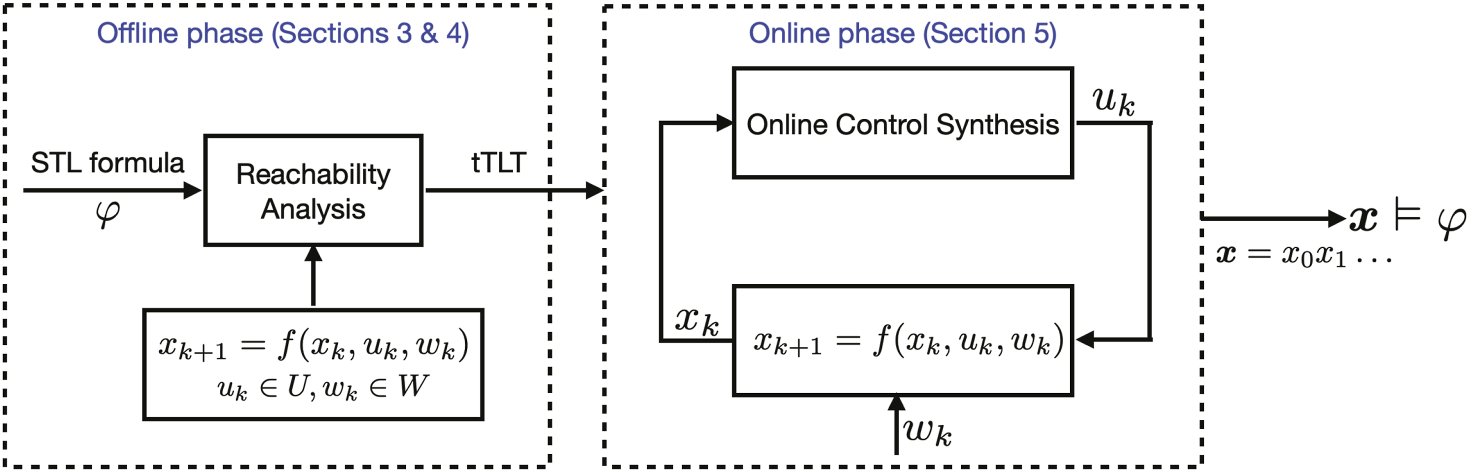
It is worth mentioning that reachability analysis is the core to ensure the robustness of the proposed algorithm, since the uncertainties in the system can be explicitly addressed when performing reachability analysis. Over the past decades, there have been remarkable progresses in the computation of reachable sets for different systems. New software tools on reachability analysis facilitate the usability of the approach proposed in our paper.
We further remark that the robustness here refers to the control ability against system uncertainties. That is, we are interested in synthesizing a controller under which the signals satisfy an STL specification despite the underlying uncertainties. This is different from the notion of quantitative robustness which measures how much a signal satisfies or violates an STL specification.
1.4. Organization and notations
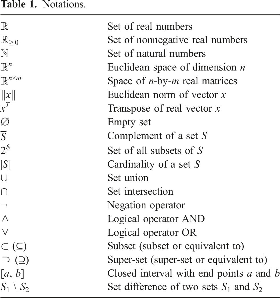
Notations.
2. Preliminaries and problem Formulation
2.1. Systems dynamics
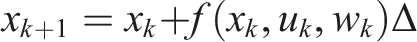
Consider an uncertain discrete-time control system of the form
A control policy One can see from Definition 2.1 that a control policy
A disturbance signal The solution of equation (1) is defined as a discrete-time signal We use The deterministic system is defined by

2.2. Signal temporal logic
We use STL to concisely specify the desired system behavior. STL (Maler and Nickovic, 2004) is a predicate logic consisting of predicates μ, which are defined through a predicate function 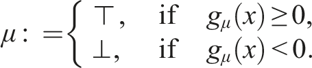
The syntax of STL is given by
The validity of an STL formula φ is originally defined with respect to a continuous-time signal (Maler and Nickovic, 2004). Later in Raman et al. (2015), the STL semantics with respect to a discrete-time signal has also been proposed. In this work, we study discrete-time control systems. Therefore, we adopt the STL semantics defined in (Raman et al., 2015).
The validity of an STL formula φ with respect to a discrete-time signal 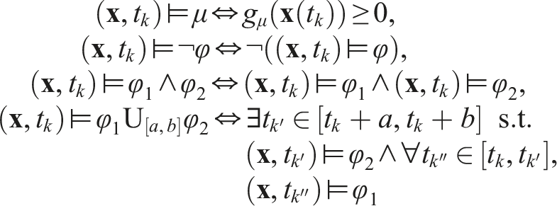
The signal
(Dokhanchi et al., 2014) The time horizon ‖φ‖ of an STL formula φ is inductively defined as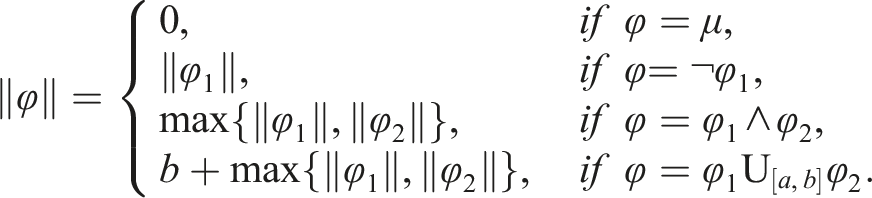
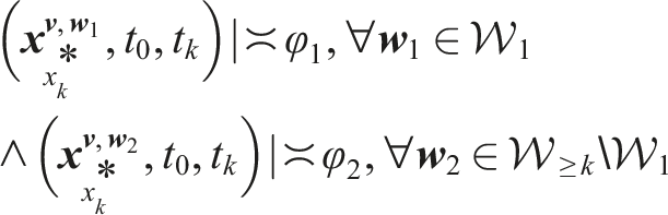
(Robust satisfiability) Consider the uncertain system equation (1) and the STL formula φ. We say φ is robustly satisfiable from the initial state x0 if there exists a control policy 
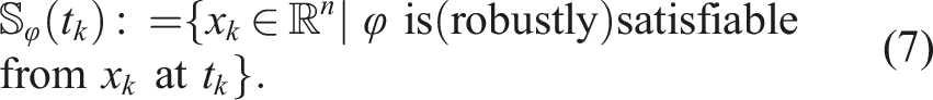
(Satisfiability) Consider the deterministic system equation (2) and the STL formula φ. We say φ is satisfiable from the initial state x0 if there exists a control policy Given an STL formula φ, the set of initial states from which φ is (robustly) satisfiable is denoted by We remark that the computation of the set 

2.3. Reachability operators
In this section, we define two reachability operators. The natural connection between reachability and temporal operators plays an important role in the approach proposed in this paper. The definitions of maximal and minimal reachable tube are given as follows.
Consider system equation (1), three sets The set 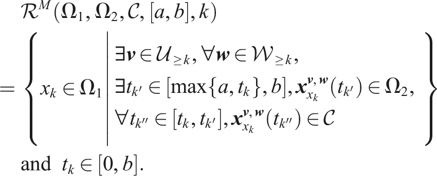
Consider system equation (1), two sets The set 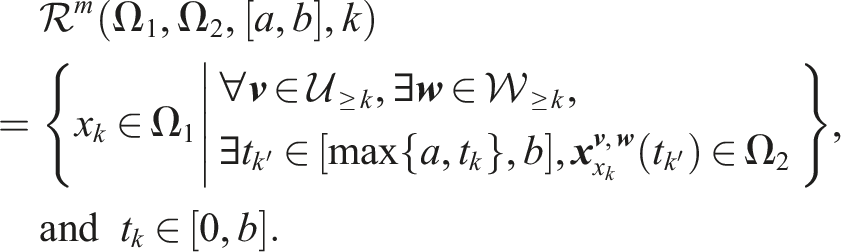
2.4. Problem formulation
Consider the following fragment of STL formulas, which is inductively defined as
The STL fragment defined in equation (5) includes nested STL formulas of the form
It is possible to handle nested STL formulas of the form The problem under consideration is formulated as follows.
Online control synthesis. Consider system equation (1) and an STL task φ in equation (5). For an initial state x0, find, if it exists, a sequence of control inputs
Note that the objective of Problem 2.1 is not to synthesize a closed-form control policy The key idea to solve Problem 2.1 is as follows. We first transform the STL formula to an alternative tree-based representation, which we call a tube-based temporal logic tree (tTLT), by leveraging reachability analysis as detailed in Section 3. There exists a semantic connection between the STL formula and the corresponding tTLT, thanks to the reachability analysis, which is explained in Section 4. Based on this fact, we can perform control synthesis over the tTLT, instead of the STL formula. An online control synthesis algorithm is provided in Section 5.
3. Real-time STL semantics and tube-based temporal logic tree
In this section, a real-time version of STL semantics and a notion of tTLT are proposed. The real-time STL semantics establish the satisfaction relation between a real-time signal and the STL formula. Based on these real-time semantics, we propose the tTLT using the close connection between STL and reachability analysis.
3.1. Real-time STL semantics
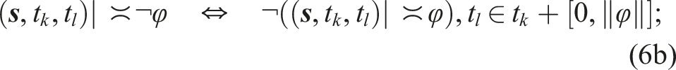
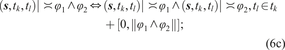
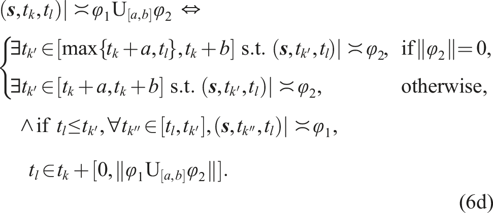
The real-time STL semantics is defined to capture the satisfaction relation between a real-time signal and an STL formula, which is different from the traditional STL semantics defined in Section 2.2. Before proceeding, the following definition is required.
Suffix and Completions. Given a discrete-time signal Given a time instant t
k
and a time interval [a, b], define t
k
+ [a, b]≔[t
k
+ a, t
k
+ b]. The real-time STL semantics is defined as follows.
Let t
k
be the starting time of any STL formula φ to be evaluated. Let t
l
≥ t
k
be the starting time of a partial signal The real-time satisfaction relation ( Using the induction rule, one can define the real-time STL semantics for “disjunction” φ1 ∨ φ2, “eventually” In parallel with Definitions 2.4 and 2.5, we define the STL satisfiability given a partial signal as follows.

Consider uncertain system equation (1) and the STL formula φ. We say φ is robustly satisfiable from the state x
k
at time t
k
if there exists a control policy 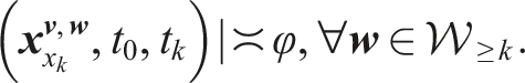
Consider the deterministic system equation (2) and the STL formula φ. We say φ is satisfiable from the state x
k
at time t
k
if there exists a control policy Note that when t
k
= t0, Definitions 3.3 and 3.4 reduce to Definitions 2.4 and 2.5, respectively. Given an STL formula φ, the set of states from which φ is robustly satisfiable at t
k
is denoted by Then, we have the following results.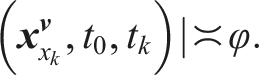
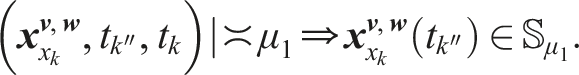
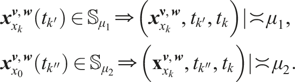
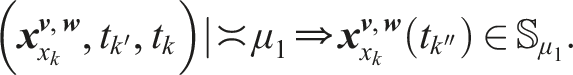
Consider system equation (1) and predicates μ1, μ2. Then, one has i) ii) iii)
First, we prove item i). Assume that • ∃tk′ ∈ [max{a, t
k
}, b], • ∀tk″ ∈ [t
k
, tk′], That is, Now we assume that Therefore, The proof of item ii) is similar and hence omitted. Next, let us prove item iii). Assume that According to Definition 2.7, In item iii) of Proposition 3.1, the use of the complementary set is motivated by the fact that
Consider system equation (1) and STL formulas φ1, φ2. If φ1 and φ2 contain no logical operators ∧ and ∨, then one has i) ii)
where
Assume that That is, Assume now that Propositions 3.1 and 3.2 imply that the real-time satisfiable set of the STL formula can be inferred by set operations and reachability analysis, which makes it reasonable to develop the tTLT, a tree structure consisting of reachable tubes and operators. In the following section, we will detail the definition of tTLT and how to construct a tTLT from a given STL formula using reachability analysis.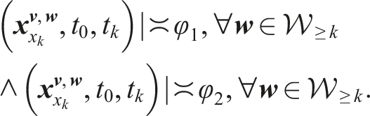
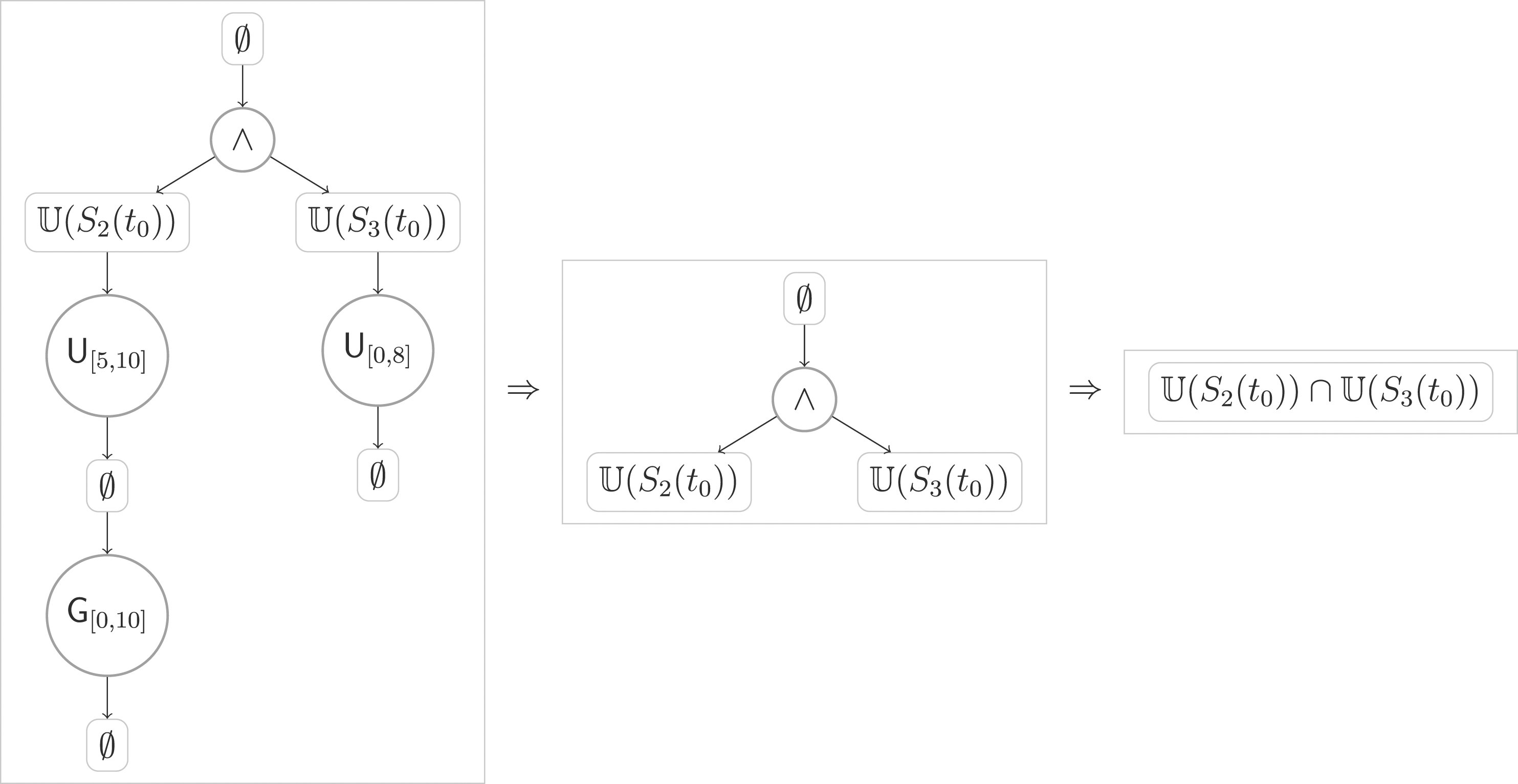
3.2. Tube-based temporal logic tree and its construction
In this section, we formally introduce the notion of tTLT and provide its construction algorithm. A tTLT is a variant of the TLT proposed in the recent work (Gao et al., 2022) for LTL formulas. Due to the time-dependent essence of STL formulas, the reachable sets in the TLT are replaced with the reachable tubes in the tTLT, which can explicitly incorporate the time constraints in STL formulas. The intuition of the tTLT is that it indicates how a state trajectory should evolve in order to satisfy the time constraints embedded in an STL formula. In the following, a formal definition of the tTLT is introduced.
A tTLT is a tree for which the following holds:
• each node is either a tube node that maps from the nonnegative time axis, i.e., • the root node and the leaf nodes are tube nodes; • if a tube node is not a leaf node, its unique child is an operator node; • the children of any operator node are tube nodes.
A complete path
The following result shows how to construct a tTLT for any given STL formula using reachability analysis.
For system equation (1) and every STL formula φ in equation (3), a tTLT, denoted by
We follow three steps to construct a tTLT.
Rewrite the STL formula φ into the equivalent positive normal form (PNF). It has been proven in Sadraddini and Belta (2015) that each STL formula has an equivalent STL formula in PNF (i.e., negations only occur adjacent to predicates), which can be inductively defined as
For each predicate μ or its negation ¬μ, construct the tTLT with only one tube node
Following the induction rule to construct the tTLT
Boolean operators ∧ and ∨. Consider two STL formulas φ
1
, φ
2
and their corresponding tTLTs
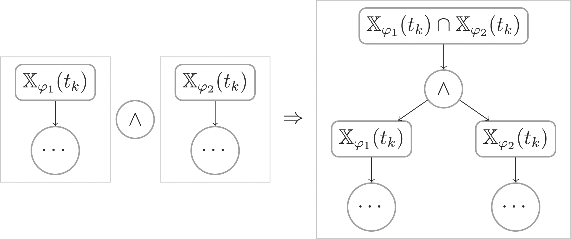
Illustrative diagram of construction tTLT for φ 1 ∧ φ 2 .
Until operator
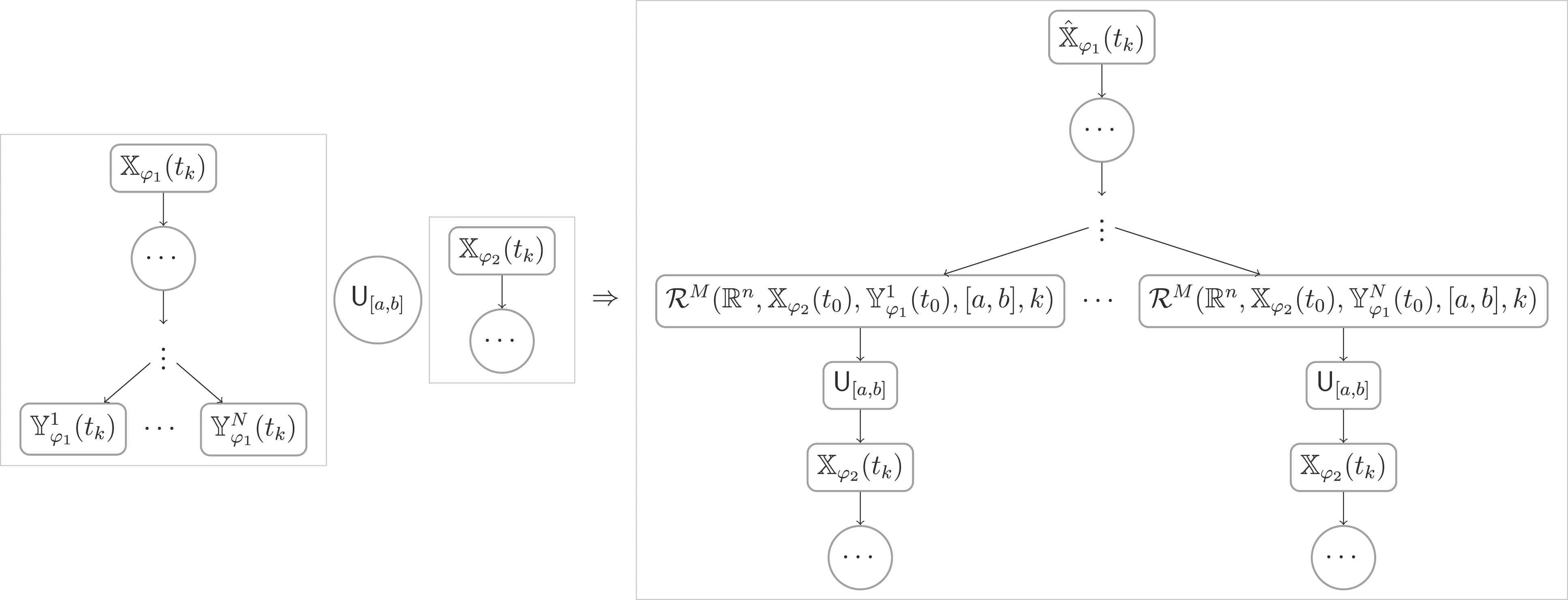
Illustrative diagram of construction tTLT for
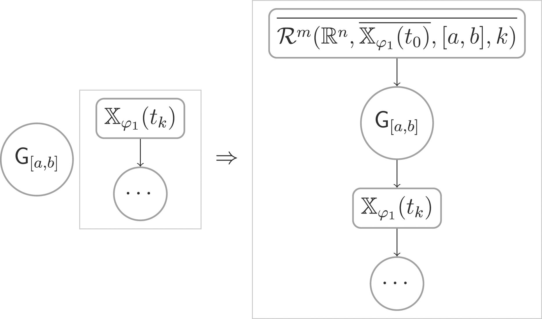
Eventually and always operators Based on Theorem 3.1, Algorithm 1 is designed for the construction of tTLT
Let us use the following example to show how to construct the tTLT.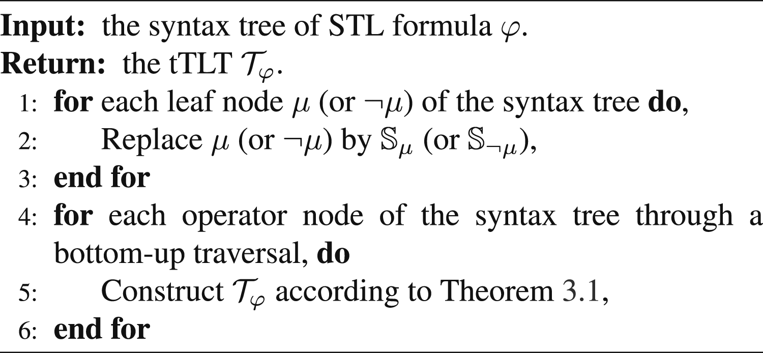
Illustrative diagram of construction tTLT for
Consider the formula
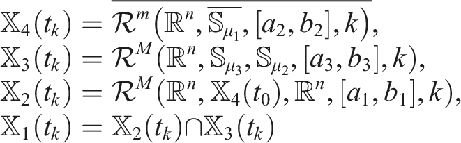
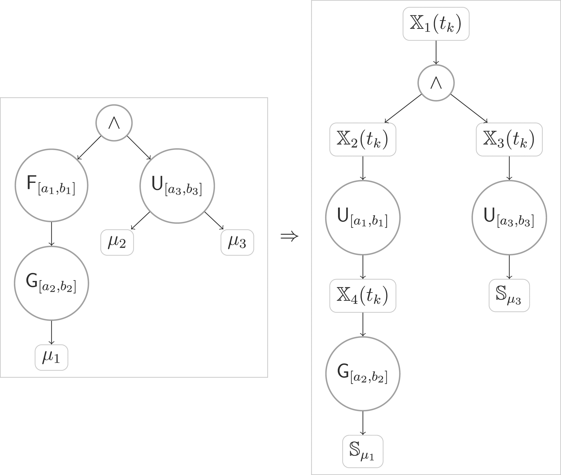
Example 3.1: syntax tree (left) and tTLT (right) for
Given an STL formula φ in PNF, let K denote the number of Boolean operators and L the number of temporal operators contained in φ. Let
4. Semantic connection between STL and tTLT
In this section, the semantic connection between an STL formula and its corresponding tTLT is derived. We define how a given state trajectory satisfies a tTLT and then show that the tTLT is a semantic under-approximation of the STL formula. Before that, let us first define the segment of the complete path.
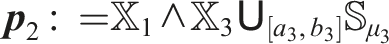
A complete path of a tTLT can be encoded in the form of
Now, we define the maximal temporal segment for a tTLT, which plays an important role when simplifying the tTLT.
A maximal temporal segment (MTS) of a complete path of the tTLT is one of the following types of segment:
1) a segment from the root node to the parent of the first Boolean operator node (∧ or ∨); 2) a segment from one child of one Boolean operator node to the parent of the next Boolean operator node; 3) a segment from one child of the last Boolean operator node to the leaf node. One can conclude from Definition 4.2 that any MTS starts and ends with a tube node and contains no Boolean operator nodes.
A time coding of (a complete path of) the tTLT is an assignment of each tube node
Now, we further define the satisfaction relation between a trajectory
Consider a trajectory
i) if Θ
i
∈ {∧, ∨}, then
ii) if
iii) if
and
iv)
v)
From items i)-iii) of Definition 4.4, one has that
With Definition 4.4, the satisfaction relation between a trajectory
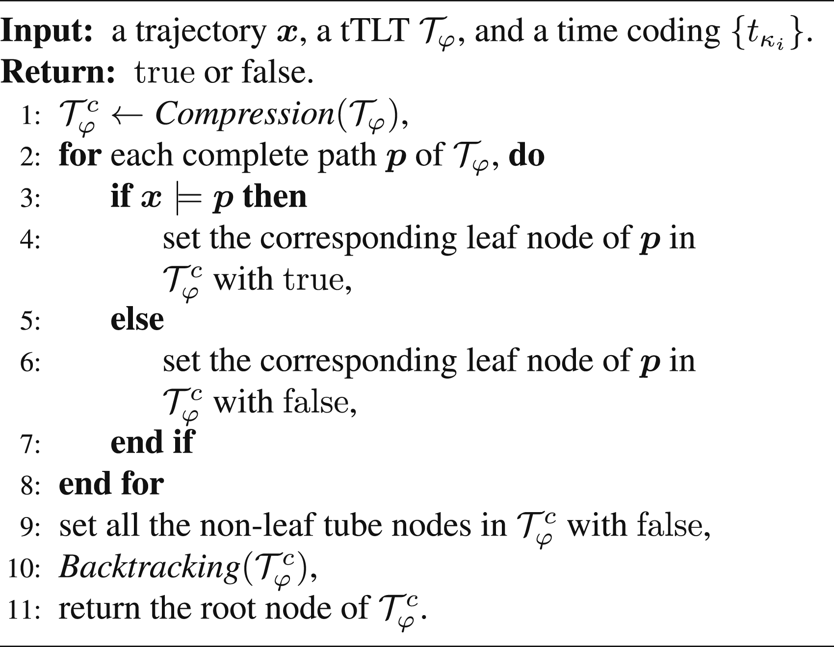
Consider a trajectory
The central idea of Algorithm 2 is to check the Boolean relation among sub-formulas of a given STL formula φ. For instance, assume
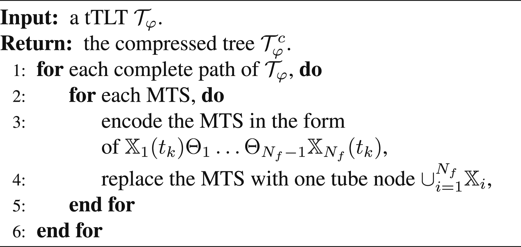
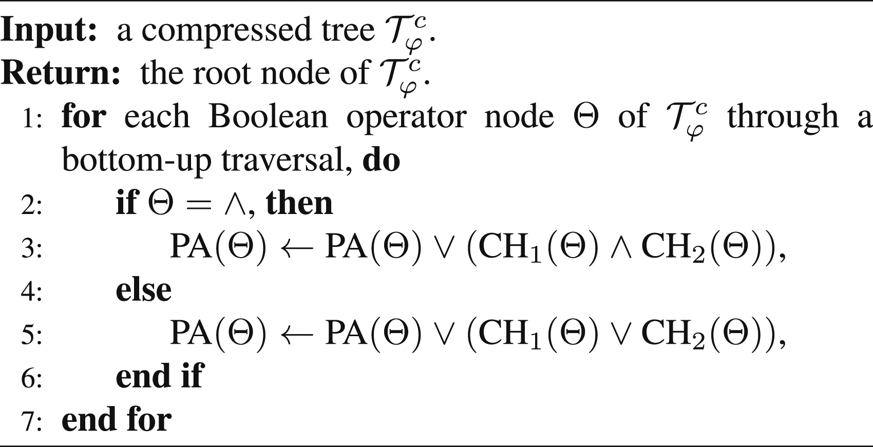
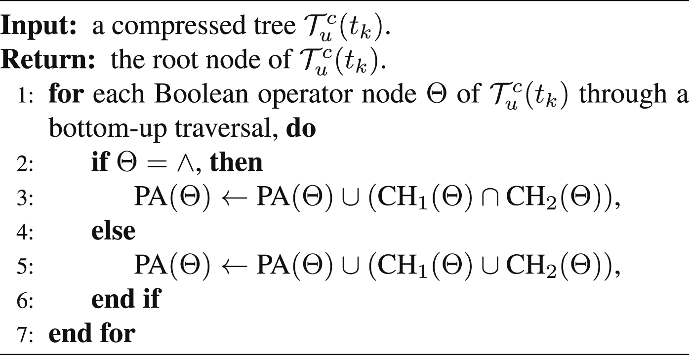
Algorithm 2 takes as inputs a trajectory We further detail the Compression algorithm (Algorithm 3) and the Backtracking algorithm (Algorithm 4) in the following. Algorithm 3 aims at obtaining a simplified tree with Boolean operator nodes and tube nodes only. To do so, we first encode each MTS in the form of
Let us continue with Example 3.1. The tTLT
And Let
Be the time coding of the complete path
In addition, the tTLT

Example 4.1: compressed tree
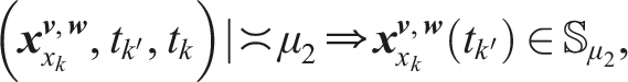
(Robustly satisfiable tTLT) A tTLT is called robustly satisfiable for system equation (1) with initial state x
0
if there exists a control policy The following theorem provides a formally semantic relation between the STL formula fragment in equation (5) and the corresponding tTLTs.
Consider the uncertain system equation (1) with initial state x
0
and an STL formula φ in equation (5). Let
From Definitions 2.4 and 4.6, one has that to prove Theorem 4.1, it is equivalent to prove
In the following, we will first prove i) ⊤, predicates μ, ¬μ, and μ
1
∧ μ
2
, μ
1
∨ μ
2
, ii) iii) iv) Case i): For ⊤, predicates μ, ¬μ, and μ
1
∧ μ
2
, μ
1
∨ μ
2
, it is trivial to verify that Case ii): We note that the proofs of the three are similar, therefore, in the following, we only consider the case Assume that Case iii): We note that the proofs of the two are similar. In the following, we consider the case Assume that Case iv): φ = φ
1
∧ φ
2
. Assume that Then, we prove v) φ
1
∨ φ
2
, where φ1 and φ2 are STL formulas belong to items ii) or iii). Case v): φ = φ
1
∨ φ
2
. The proof of The proof of Thanks to the semantic relation between the STL formulas in equation (5) and their corresponding tTLTs, we are able to perform control synthesis over the tTLT, instead of the STL formulas, with correct-by-construction guarantees. The details of this control synthesis are provided in the next section.
where φ1 and φ2 in item iv) are STL formulas belong to items ii) or iii).
tTLTs
tTLTs for
5. Online control synthesis
In this section, we study the STL control synthesis problem in Problem 2.1. In the following, an online control synthesis algorithm and its sub-algorithms are designed over the tTLT such that the tTLT
5.1. Definitions and notations
Before proceeding, the following definitions and notations are needed.
The time horizon |Θ| of an STL operator 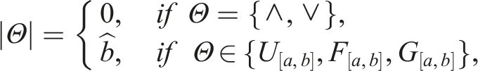
A segment of a complete path of a tTLT is called a Boolean segment if it starts and ends with a tube node and contains only Boolean operator nodes. We say a tube node
If each node of a tree is either a set node that is a subset of U or an operator node that belongs to
Each tube node
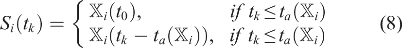
• • Denote by Moreover, one has that
At each time instant t
k
,
• P(t
k
): the set which collects all the set nodes of, i.e., P(t
k
) = ∪
i
S
i
(t
k
),
• Θ: the set which collects all the operator nodes of
For a node N
i
(t
k
) ∈ P(t
k
) ∪ Θ, define
• CH(N
i
(t
k
)): the set of children of node N
i
(t
k
),
• PA(N
i
(t
k
)): the set of parents of node N
i
(t
k
),
•
•
Given a state-time pair (x
k
, t
k
), define


5.2. Online control synthesis
In the following, we present the online control synthesis algorithm (and its sub-algorithms), and then present an example to further explain how each sub-algorithm works.
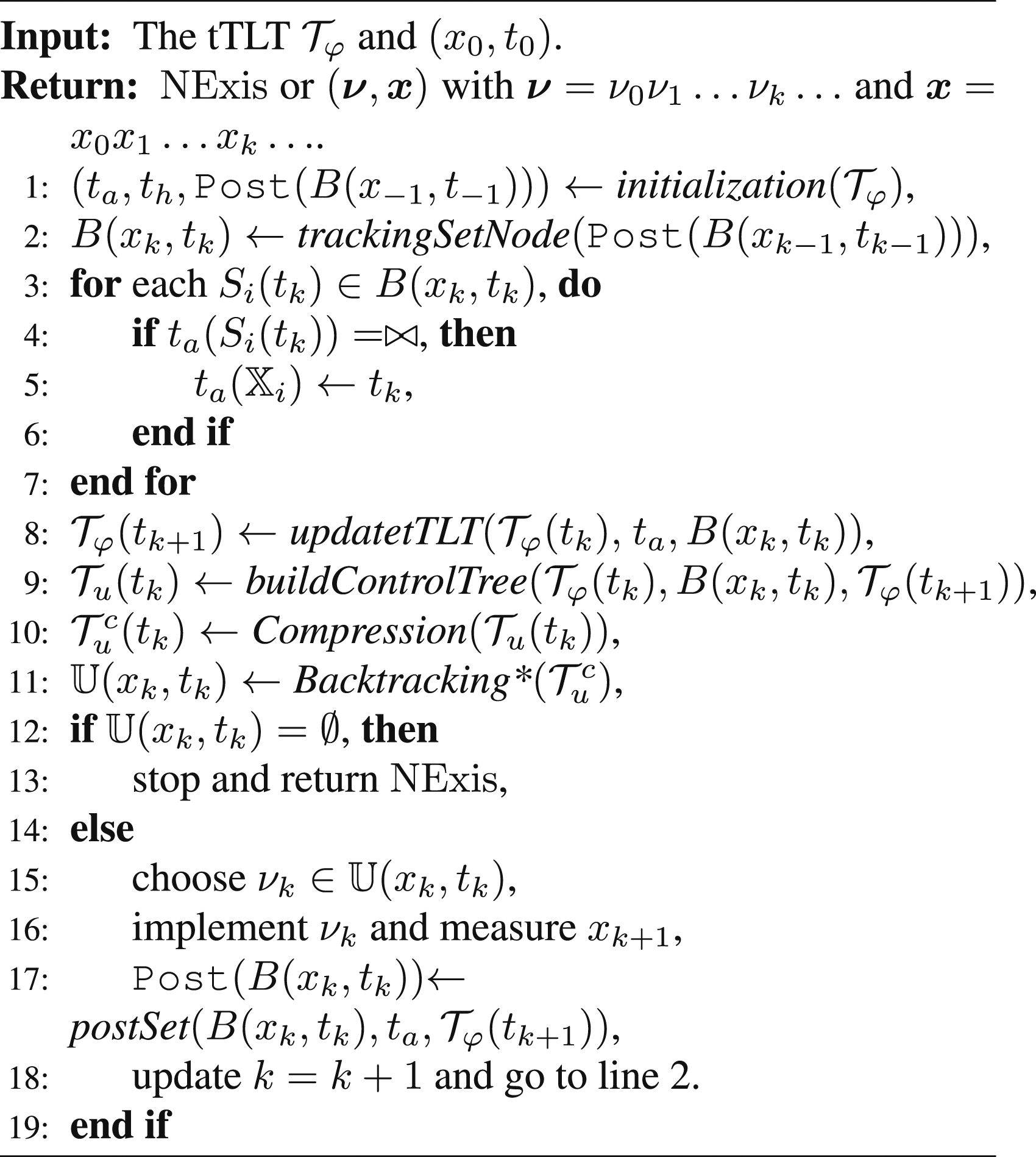
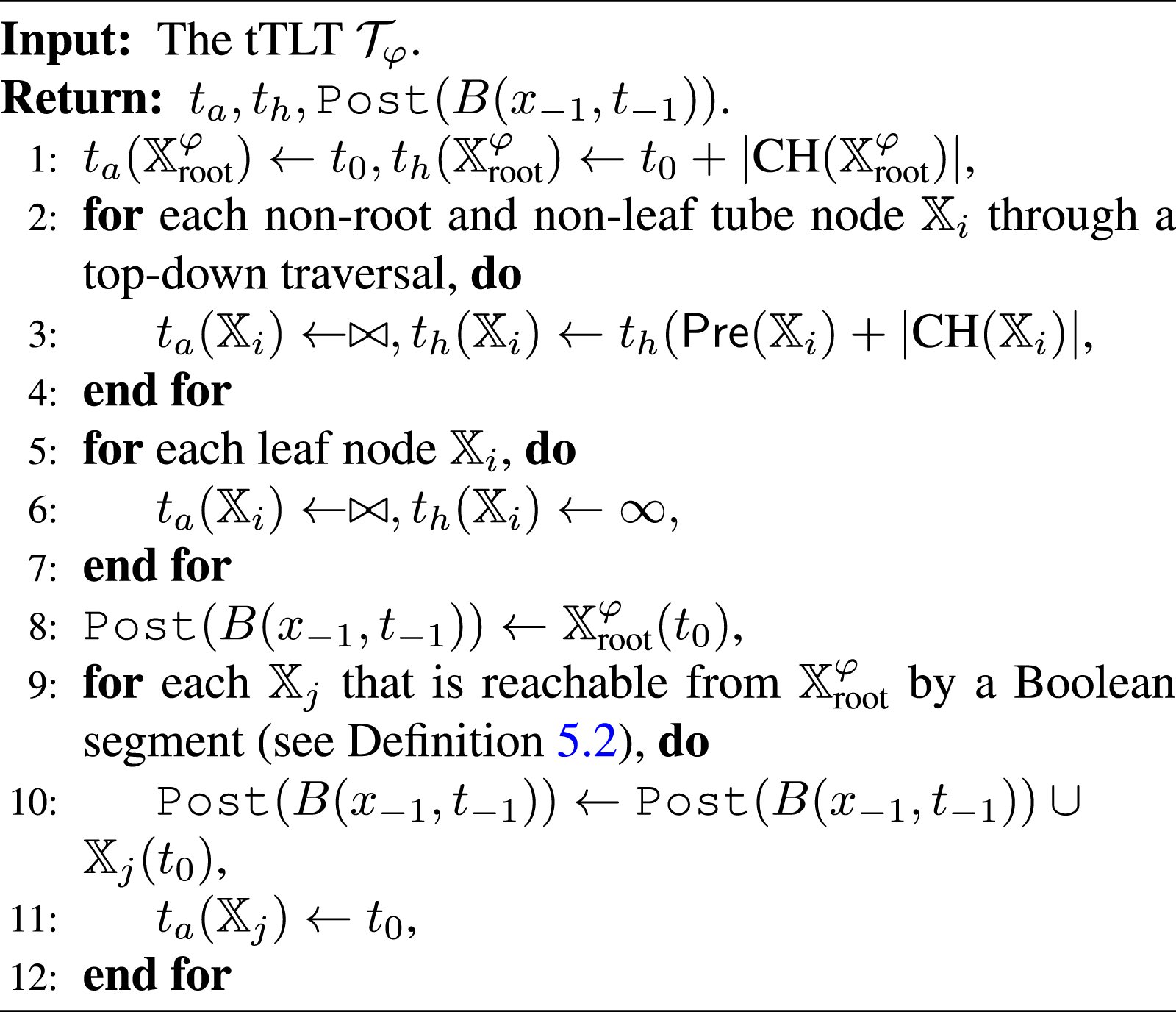
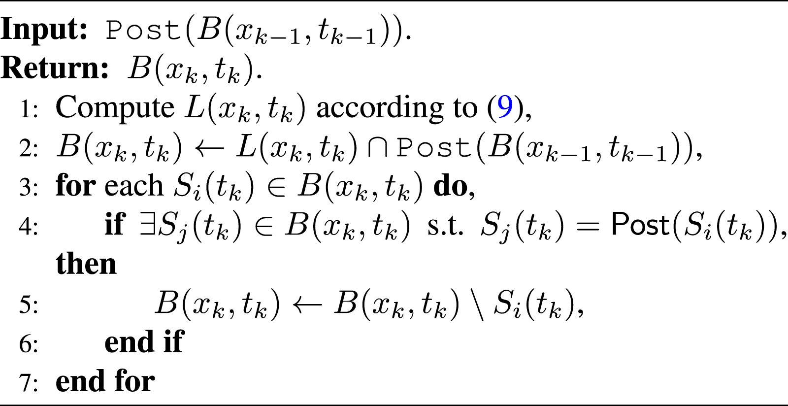
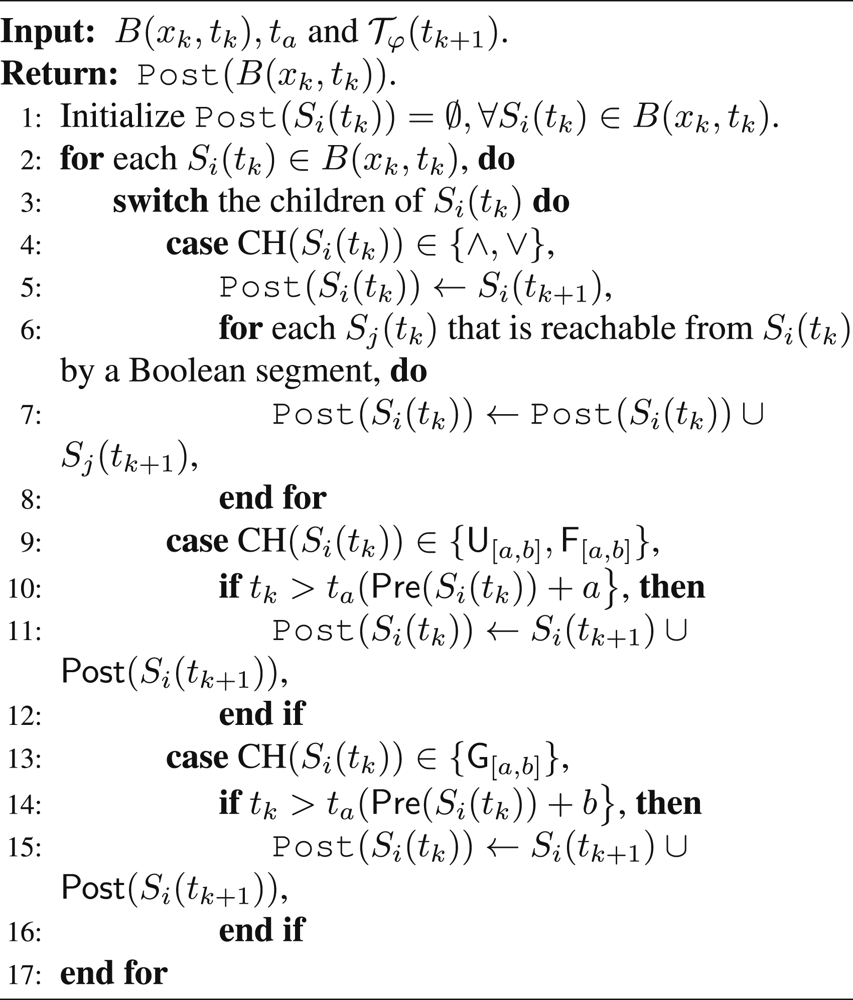
The online control synthesis algorithm is outlined in Algorithm 5. Before implementation, an initialization process (line 1) is required, which is outlined in Algorithm 6. Here, t
a
and t
h
are two functions that map each tube node
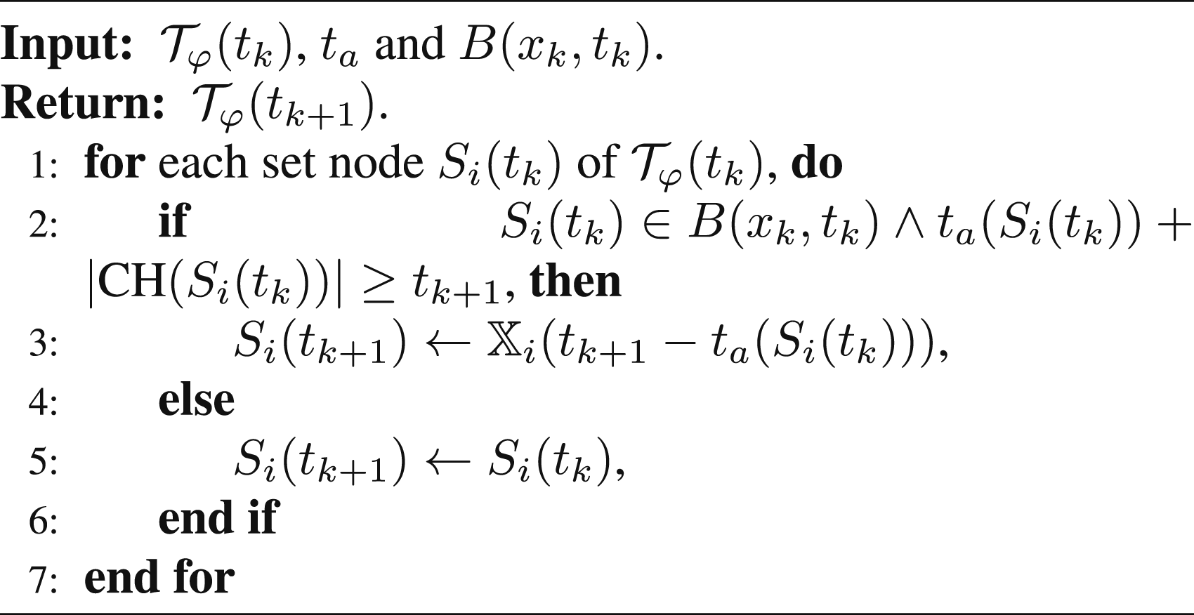
We further detail Algorithms 6–11 in the following. • Algorithm 6 calculates the functions t
a
and t
h
(lines 1-7) and • Algorithm 7 outlines the procedure of finding the subset of set nodes in P(t
k
) that are valid at time t
k
, i.e., B(x
k
, t
k
). This is the most important step of the control synthesis, and it relates to Algorithm 11 postSet. Firstly, one needs to compute the subset of set nodes of P(t
k
) that contains x
k
at time t
k
, i.e., L(x
k
, t
k
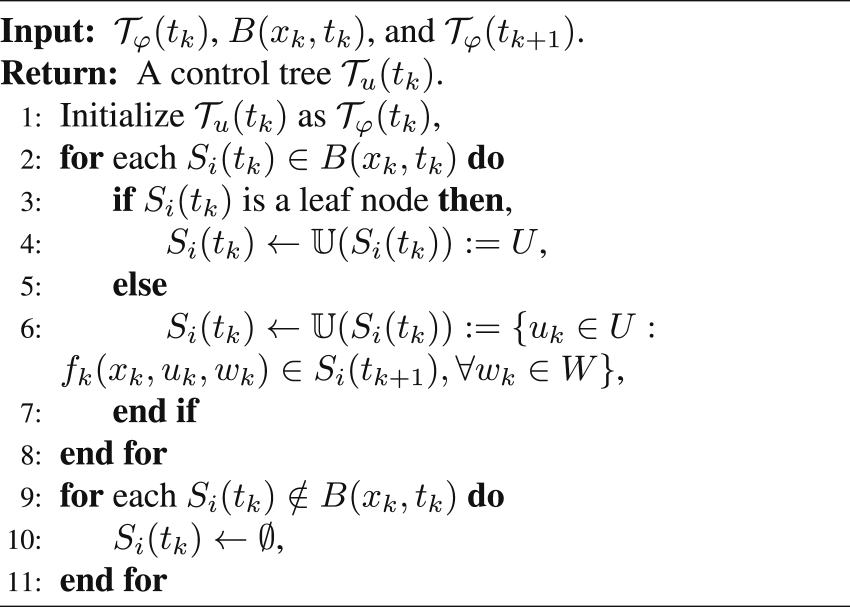
) (line 1). Then, one has from Definition 4.4 that if a trajectory • Algorithm 8 outlines the procedure of calculating • Algorithm 9 outlines the procedure of building a control tree • Algorithm 10 is similar to Algorithm 4, which outlines the procedure of backtracking a compressed tree. • Algorithm 11 outlines the procedure of finding the subset of set nodes that are possibly available at the next time instant t
k+1
given B(x
k
, t
k
), t
a
and
Next, an example is given to illustrate one iteration of the control synthesis algorithm (Algorithm 5).
Consider the single-integrator control system
The tTLT that corresponds to φ is plotted in
Figure 5
. Using Definitions 2.6 and 2.7, one can calculate that
The initial state x
0
= [0.5,0.8]
T
, for which
And
Now, let us see how the feasible control set
1) Find B(x
0
, t
0
) via Algorithm 7. First, L(x
0
, t
0
) is computed according to equation (9), Then, after running lines 2-7, one has 2) Determine the activation time. Initially, both 3) Update the TLT (thus obtain 4) Build the control tree Since The following theorem shows the applicability and soundness of Algorithm 5.


Left:
Consider uncertain system equation (1) with initial state x
0
and an STL formula φ in equation (5). Assume that φ is robustly satisfiable for equation (1) and (i) the control set (ii) the resulting trajectory
The proof follows from the construction of tTLT and Algorithms 5-11. The existence of a controller ν
k
at each time step t
k
, is guaranteed by the definition of maximal and minimal reachable sets (Definitions 2.6 and 2.7), and the construction of tTLT (Propoition 3.1, Theorem 3.1 and Algorithm 1). Moreover, the design of Algorithms 5-11 guarantees that the resulting trajectory
The tTLT construction relies on the computation of backward reachable tubes. Over the past decade, new approaches (e.g., decomposition-based approach (Chen et al., 2018a) and learning-based approaches (Allen et al., 2014; Bansal and Tomlin, 2021)) and software tools (e.g., Hamilton-Jacobi Toolbox (Mitchell and Templeton, 2005) and CORA Toolbox (Althoff, 2015)), have been developed for improving the efficiency of computing backward reachable tubes. Moreover, we remark that the computation of reachable tubes in our work for constructing of the tTLT can be performed offline, which may mitigate the online computational burden. On the other hand, although the exact computation of backward reachable sets/tubes is in general nontrivial for high-dimensional nonlinear systems, efficient algorithms exist for linear systems with polygonal input and disturbance sets (Kurzhanski and Pravin, 2014).
The online control synthesis algorithm (Algorithm 5) contains 7 sub-algorithms, i.e., Algorithm 3 and Algorithms 6-11. The computational complexity is determined by Algorithm 9, in which one-step feasible control sets need to be computed. The computational complexity of Algorithms 3, 6, 7, 8, 10, 11 is
Different from the mixed-integer programming formulation for STL control synthesis (Raman et al., 2014, 2015), where an entire control policy has to be synthesized at each time step, the control synthesis in our work is reactive in the sense that only the control input at the current time step is generated at each time step.
6. Numerical simulations
In this section, two examples illustrating the theoretical results are provided. We first perform a numerical simulation for car overtaking. We then apply our algorithms to motion planning of a mobile robot over a group of STL specifications and test the scalability of our algorithms with respect to the growing STL complexity.
6.1. Car overtaking example
We first consider a car overtaking example. This example will specify an overtaking task as an STL formula and then show how to synthesize an overtaking controller with safety guarantees.
As shown in Figure 10, we consider a scenario where an automated vehicle Veh1 plans to move to a target set Scenario illustration: an automated vehicle plans to reach a target set 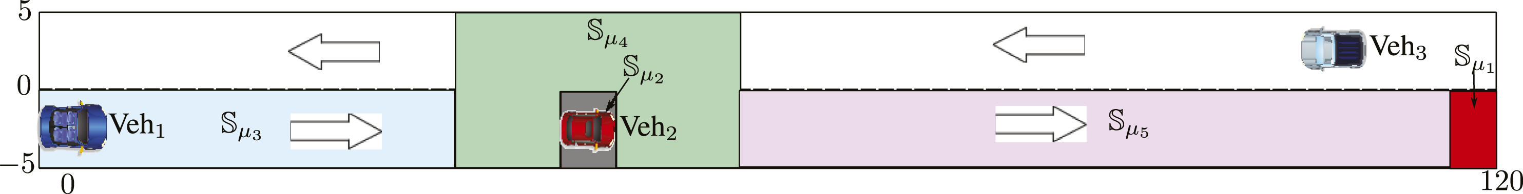
We describe the dynamics of the vehicle Veh1 as in Murgovski and Sjöberg (2015):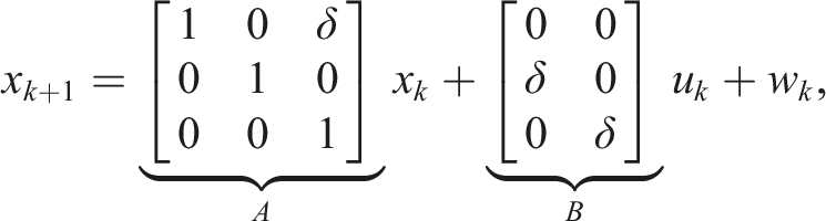
We use 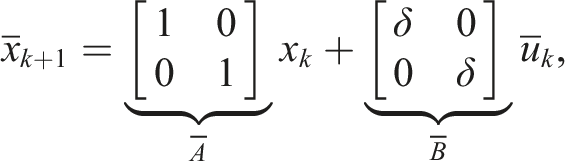
To formulate the overtaking task, we define the following three sets as shown in Figure 10:
Let us choose the sampling period as δ = 0.2s(seconds). To respect the time constraint and the input constraint for Veh1, we consider two possible solutions to the previous reachability problem: (1) fast overtaking: overtake Veh2 before Veh3 passes Veh2; (2) slow overtaking: wait until Veh3 passes Veh2 and then overtake Veh2. The fast overtaking can be encoded into an STL formula: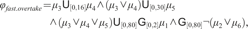
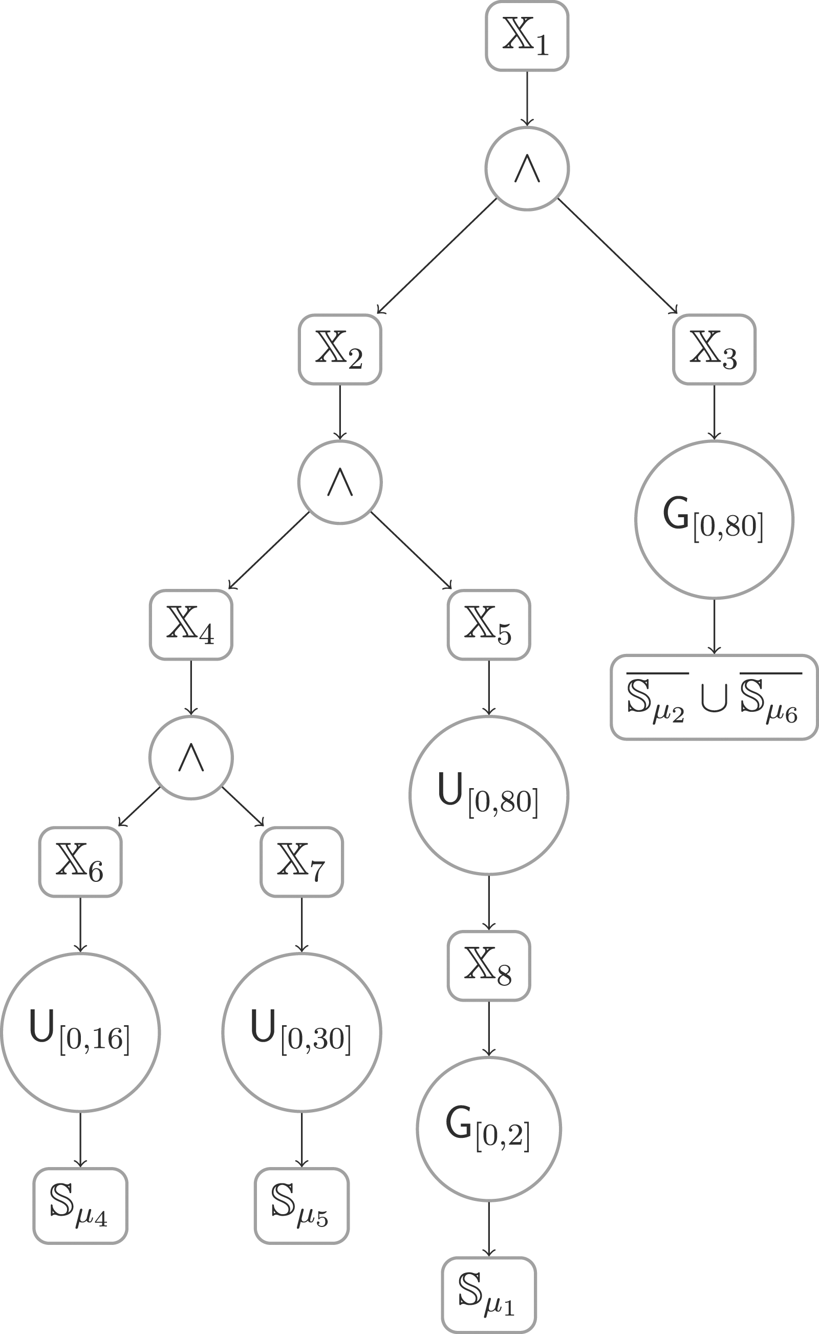
where The constructed tTLT 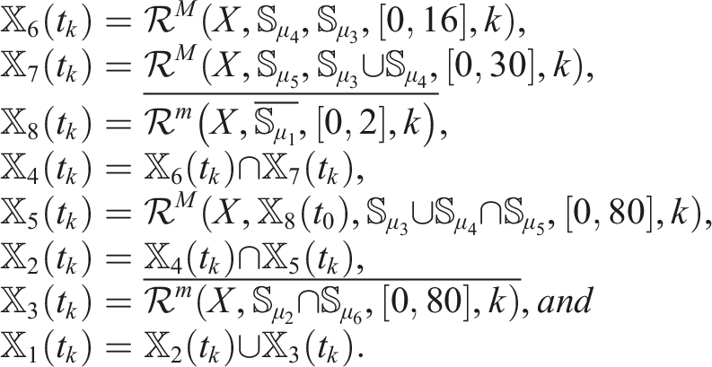
The slow overtaking can be encoded into an STL formula
In the following, two simulation cases are considered and the online control synthesis algorithm is implemented. In the fast overtaking, we choose the initial position Trajectories for one realization of disturbance signal in the fast overtaking: (a) position trajectory; (b) velocity trajectory of x-axis; (c) control trajectory of x-axis; (d) control trajectory of y-axis. Trajectories for one realization of disturbance signal in the slow overtaking: (a) position trajectory; (b) velocity trajectory of x-axis; (c) control trajectory of x-axis; (d) control trajectory of y-axis.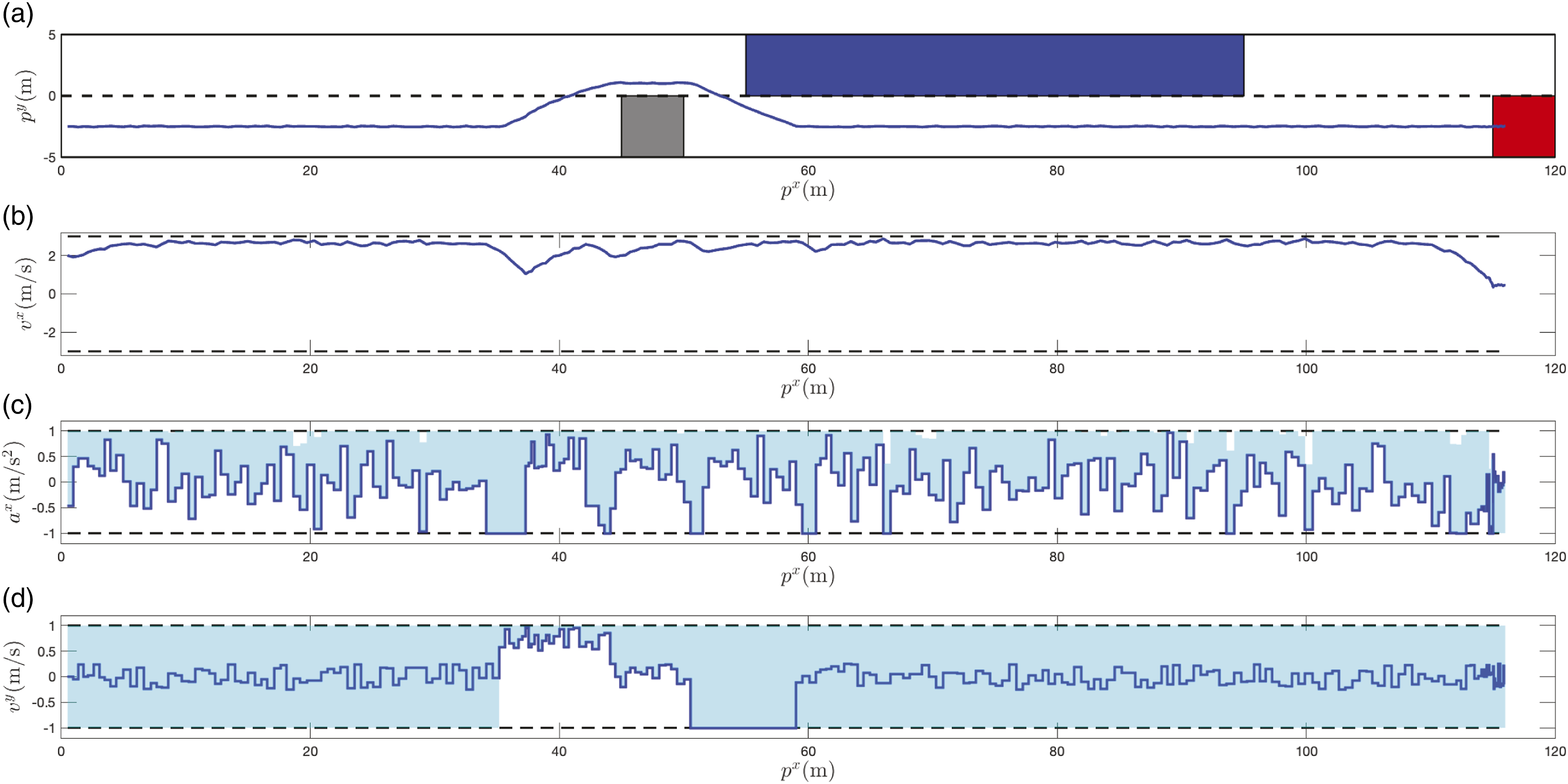
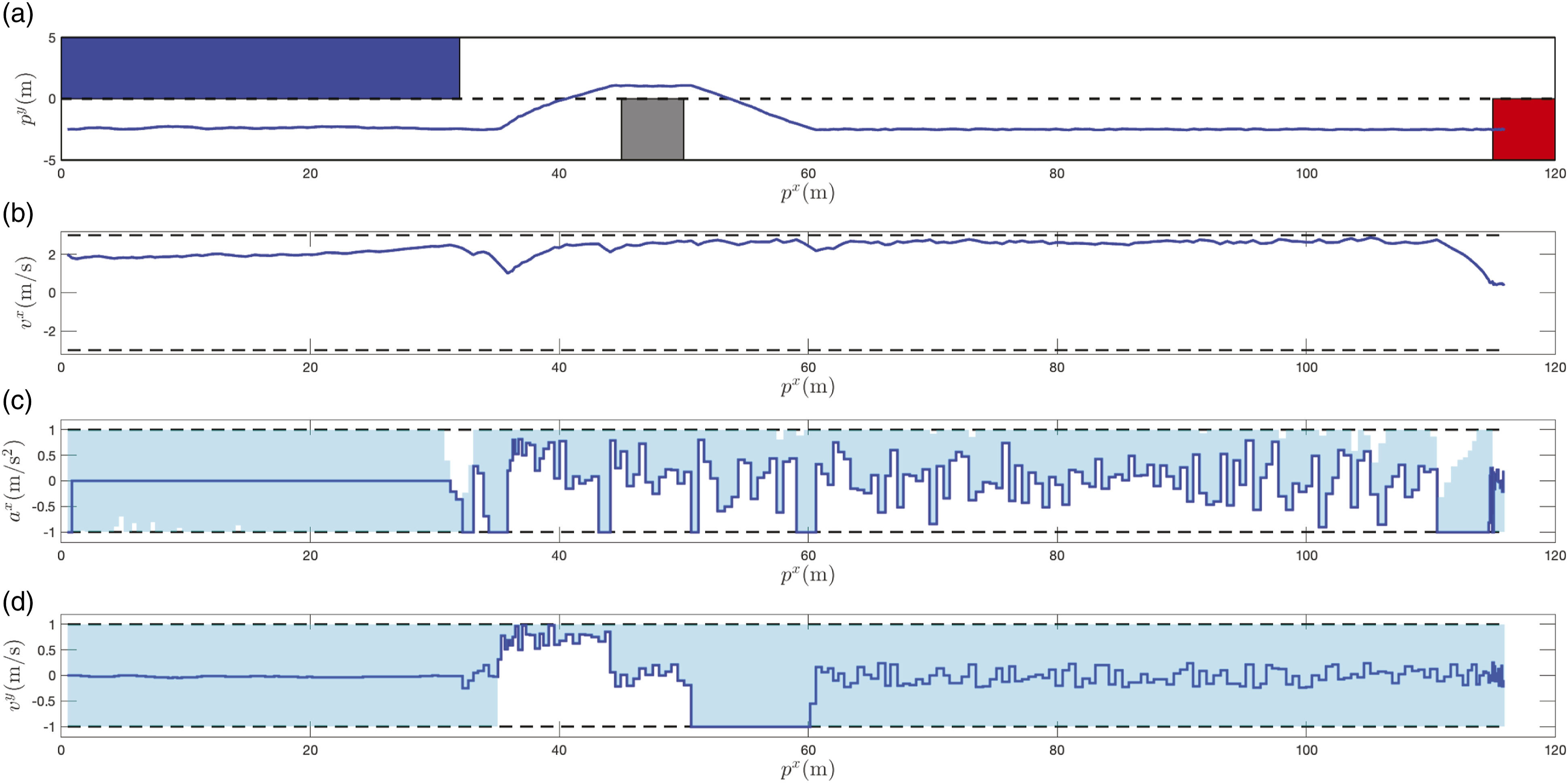
To highlight the effect of disturbances, we compare the trajectories with and without disturbances in the fast overtaking, which are shown in Figure 14(a)–(e). In Figure 14(a), we show the evolution of the x-axis position along the time. We use k
1
, k
2
, and k
3
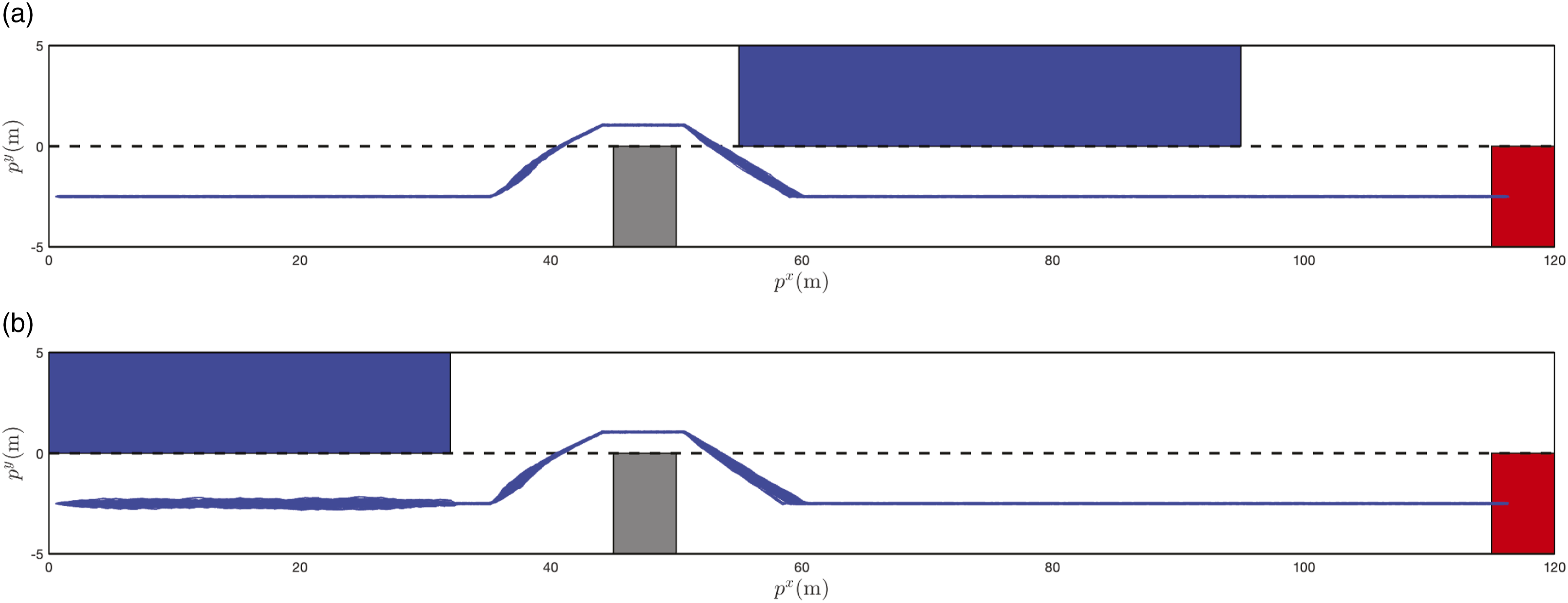
(or Comparison of robust control with noise and deterministic control without disturbance signal in the fast overtaking: (a) position-time trajectory; (b) velocity trajectory of x-axis; (c) control trajectory of x-axis; (d) control trajectory of y-axis; (e) disturbance signals. Comparison of robust control with noise and deterministic control without disturbance signal in the ast overtaking in the slow overtaking: (a) position-time trajectory; (b) velocity trajectory of x-axis; (c) control trajectory of x-axis; (d) control trajectory of y-axis; (e) disturbance signals. Position trajectories for 100 realizations of disturbance signals. (a) Position trajectories for 100 realizations of disturbance signals in the fast overtaking. (b) Position trajectories for 100 realizations of disturbance signals in the slow overtaking.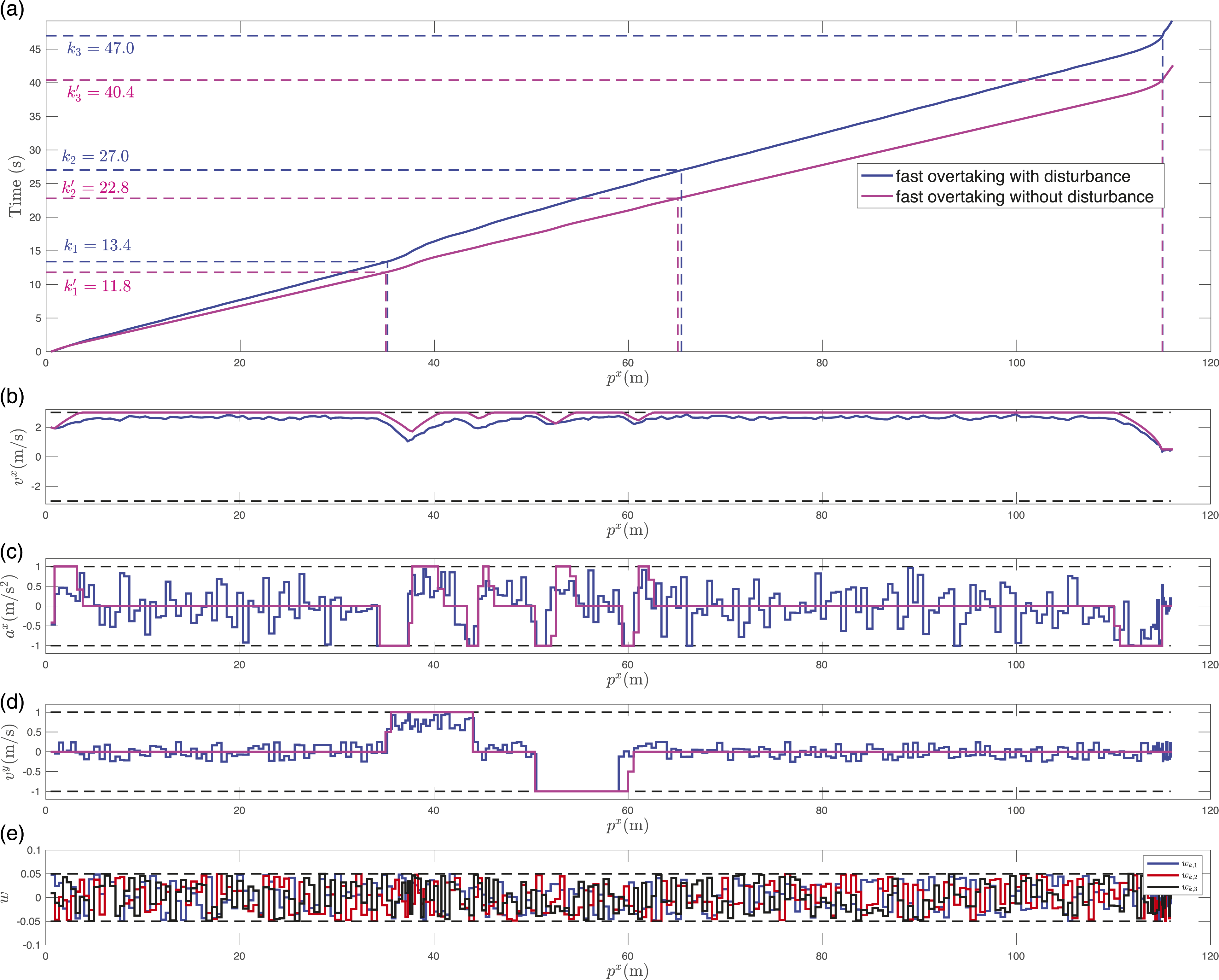
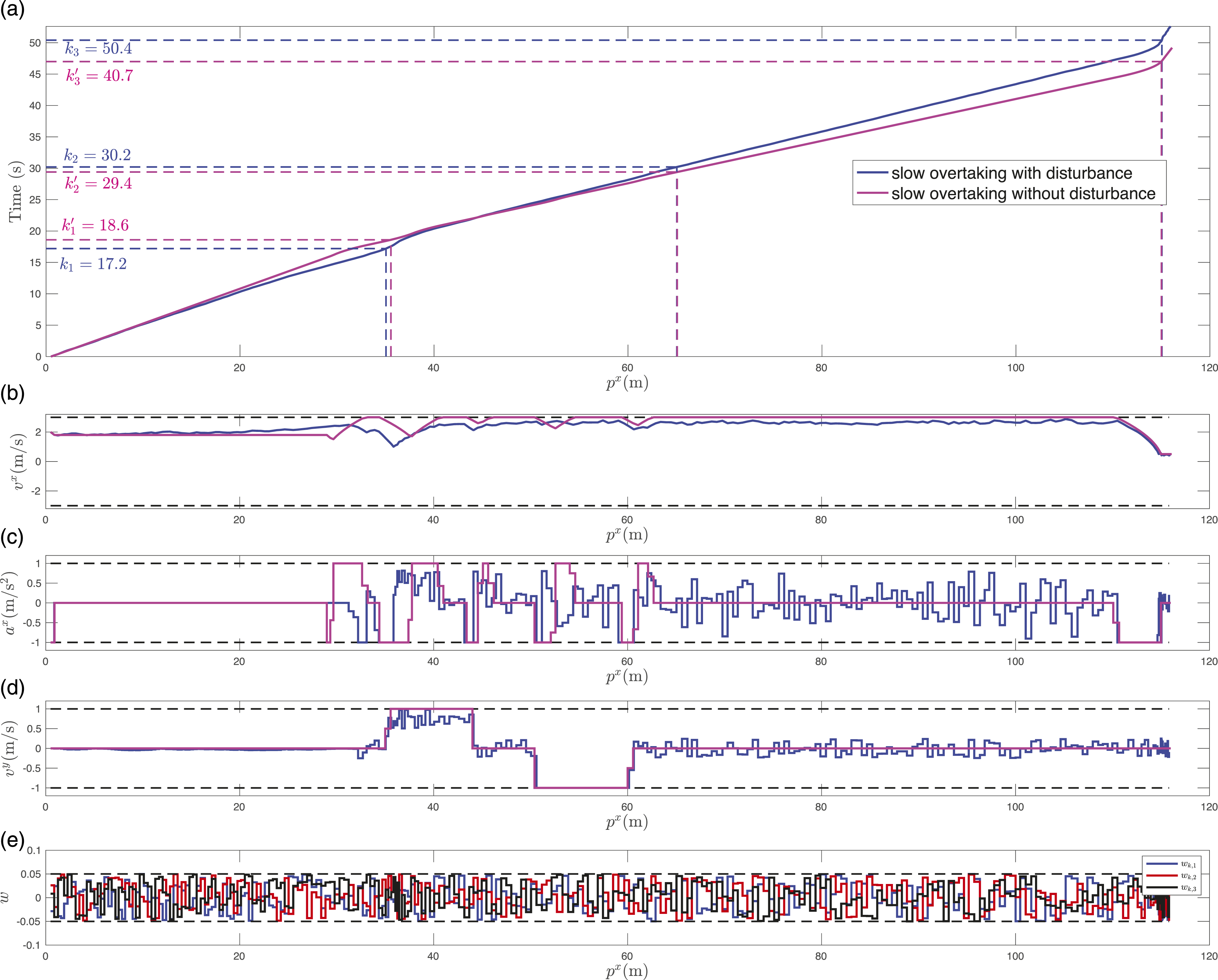
Finally, we report the computation time of this example, which was run in Matlab R2016a with MPT toolbox (Herceg et al., 2013) on a Dell laptop with Windows 7, Intel i7-6600U CPU 2.80 GHz and 16.0 GB RAM. We perform reachability analysis for constructing the tTLT offline, which takes 59.10 s. For online control synthesis, the minimal computation time at a single time step over 100 realizations is 0.23 s, while the maximal computation time is 1.07 s. The average time of each time step is 0.31 s. We remark that the mixed-integer formulation is difficult to implement in this example. This is because the computational complexity of mixed-integer programming grows exponentially with the horizon of the STL formula, which in this example reaches up to 400 sampling instants, much longer than the horizons considered in the simulation examples of Raman et al. (2015, 2014); Sadraddini and Belta (2015).
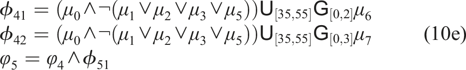
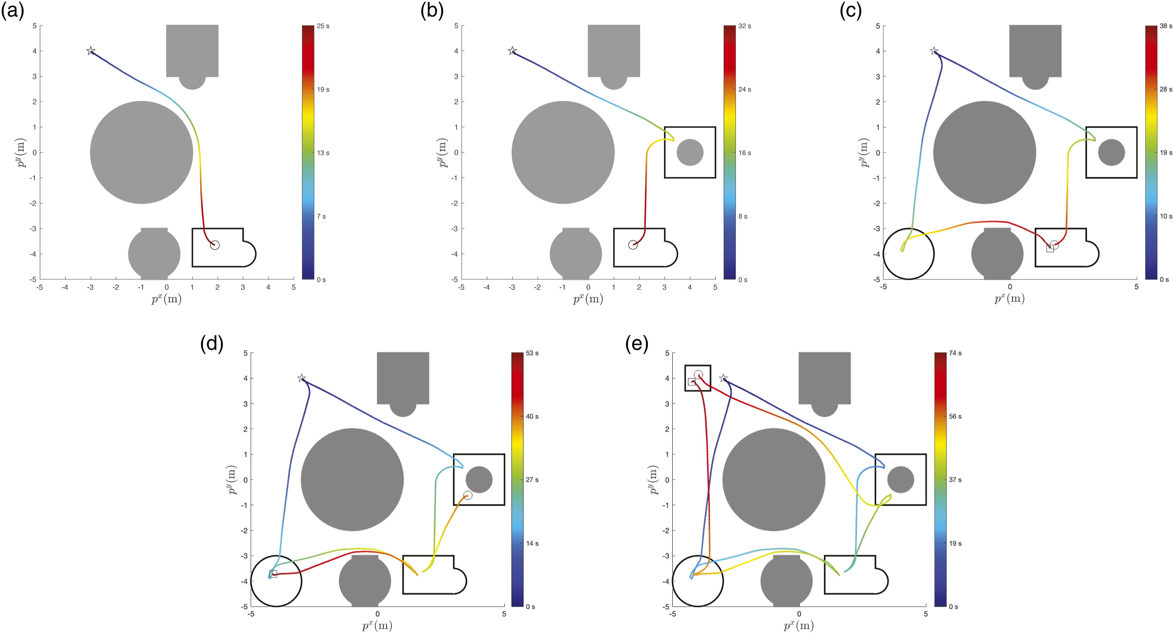
6.2. Motion planning example
In this section, we consider the motion planning of a mobile robot in an environment, as shown in Figure 17, under a group of STL specifications with growing complexity. We describe the underlying continuous dynamics of the automated vehicle as: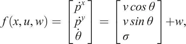

We set Δ = 0.05s.
We consider the following five STL formulas φ
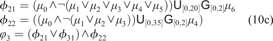
i
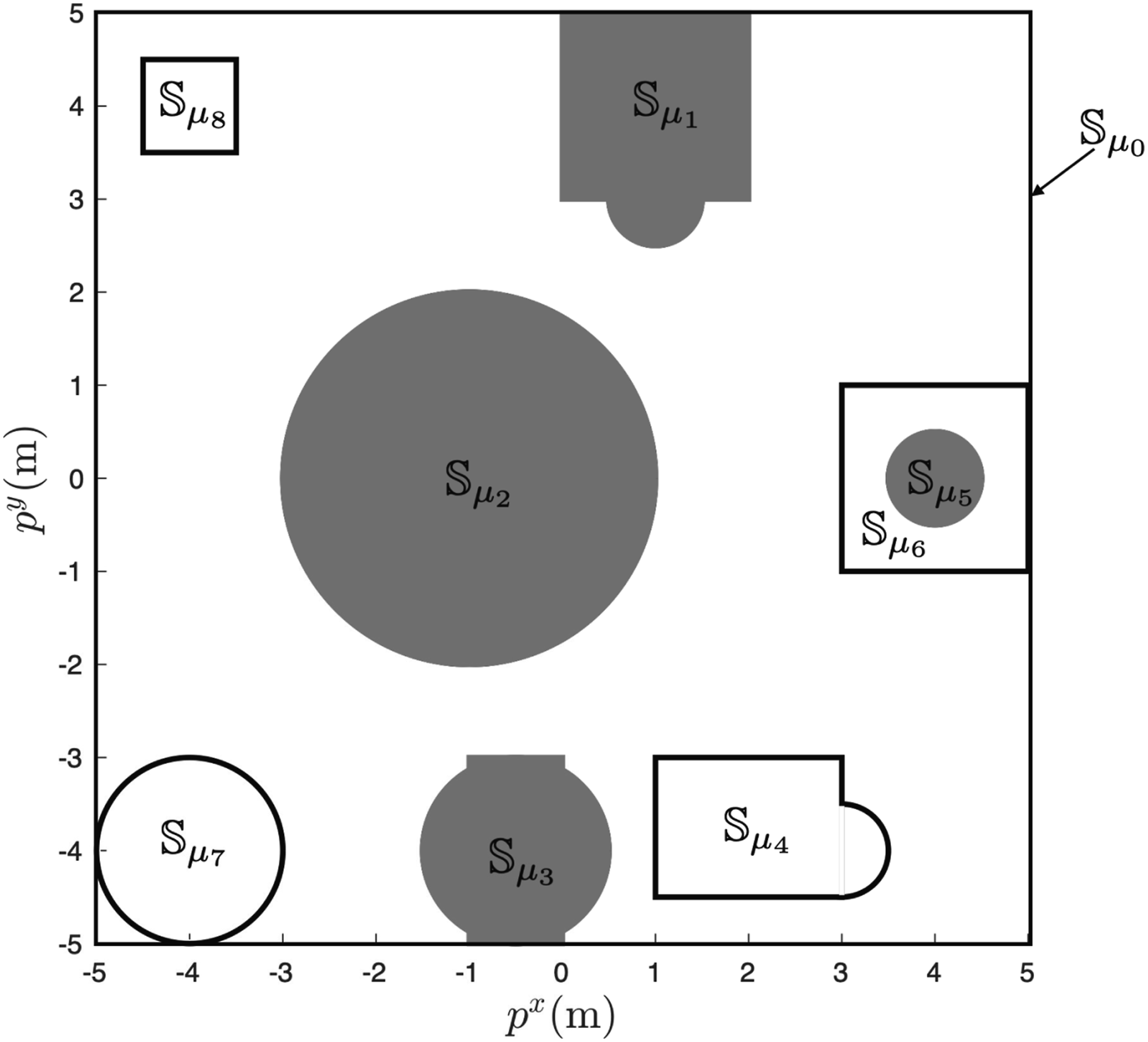
, i = 1, …, 5, as defined in equations (10a)–(10e). These five formulas have increasing complexity, e.g., longer horizon and more operators. We report the computation time of this example, which was run in Matlab R2022b with the Level Set Method Toolbox (Mitchell and Templeton, 2005). The offline computation time for constructing the tTLT and the online computation time for synthesizing the controller are summarized in Table 2. As expected, the offline computation time typically increases with respect to the complexity of STL formulas. Note that the formulas φ
3
and φ
4
have the same computation time (134.49 s) since the computation of reachable sets for ϕ
3
can be directly reused to construct the tTLT of ϕ
4
, despite that ϕ
4
looks more complex than ϕ
3
. On the other hand, the online computation for control synthesis, measured by the computation time per time step, is very efficient for all the formulas. The position trajectories are plotted in Figure 18, where the initial position is indicated by the star and the end position is the circle. The time information over the trajectories is illustrated by the color map. Scenario illustration: an automated vehicle needs to enter into the parking lot, park in the designated parking spot (blue), and leave the parking lot, while avoiding any collisions. Computation time under different STL formulas. The position trajectories that fulfill the STL formulas φ
i
, i = 1, …, 5. The time information is indicated using different colors. (a) A position trajectory that fulfill φ
1
(b) a position trajectory that fulfills φ
2
(c) two position trajectories that fulfills φ
3
(d) two position trajectories that fulfills φ
4
(e) two position trajectories that fulfills φ
5
.


7. Car parking experiment
In this section, we consider a car parking example. This example will specify a parking task as an STL formula and then show how our algorithms perform on real hardware. We will first perform reachability analysis for constructing the tTLT offline and then we use the tTLT to synthesize a parking controller for the Small-Vehicles-for-Autonomoy (SVEA) platform (Jiang et al., 2022).
As shown in Figure 19, we consider a scenario where an automated vehicle must enter the parking lot Scenario illustration: an automated vehicle needs to enter into the parking lot, park in the designated parking spot (blue), and leave the parking lot, while avoiding any collisions.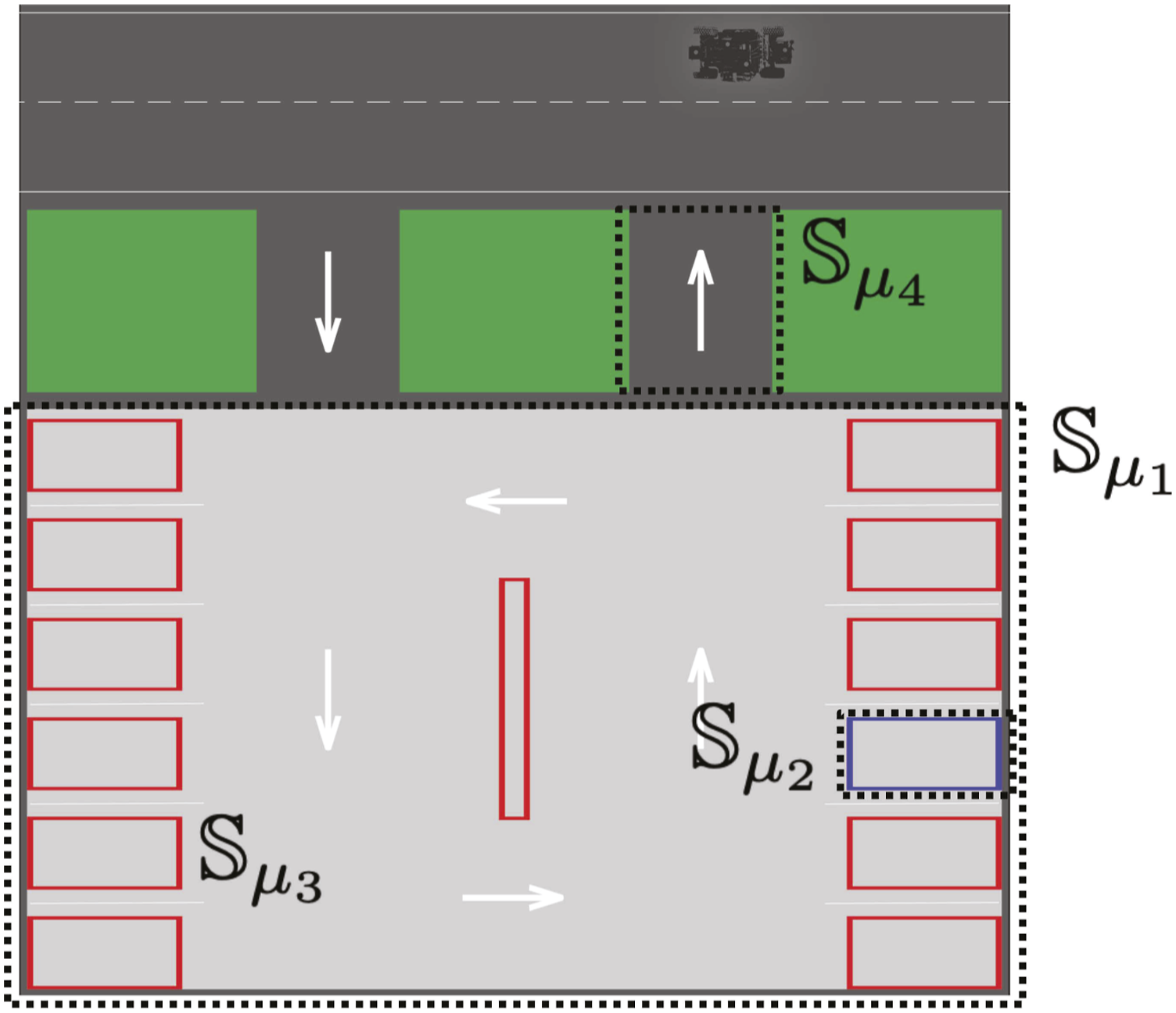
We describe the underlying continuous dynamics of the automated vehicle as: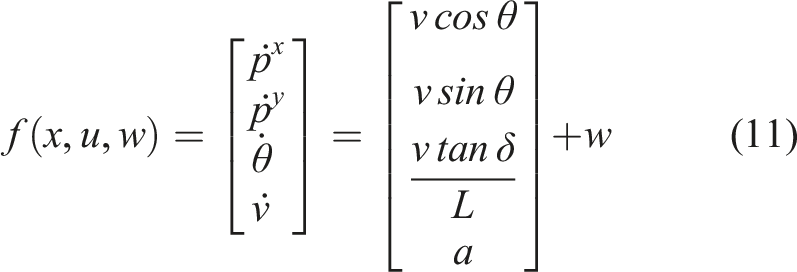
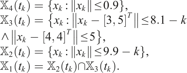
For the parking task, we set Δ = 0.05s. We define the state sets in Figure 19 as
We let the full scenario be 60 s long and specify that the vehicle needs to enter the parking lot, park in the designated spot, and leave the parking lot within 10 s, 40 s, and 60 s, respectively. Then, this parking task can be encoded into the following STL formula: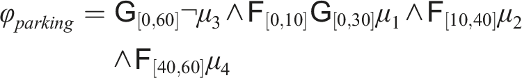
First, we use Algorithm 1 to construct the corresponding tTLT The constructed tTLT 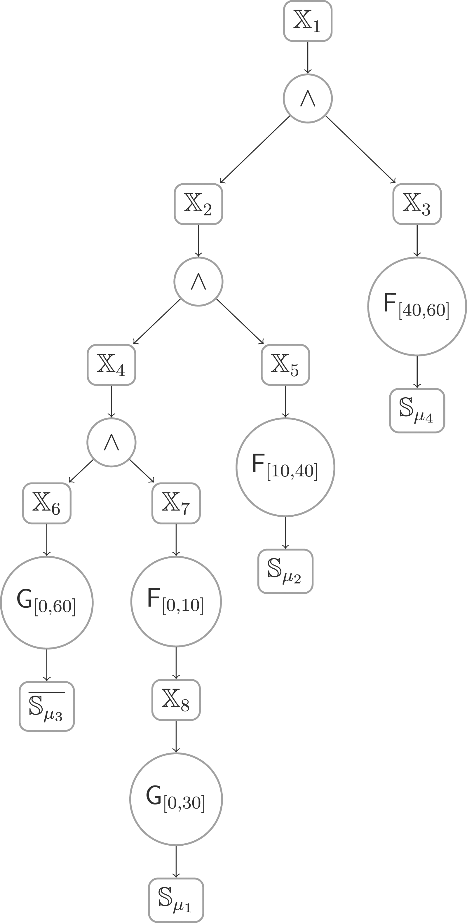
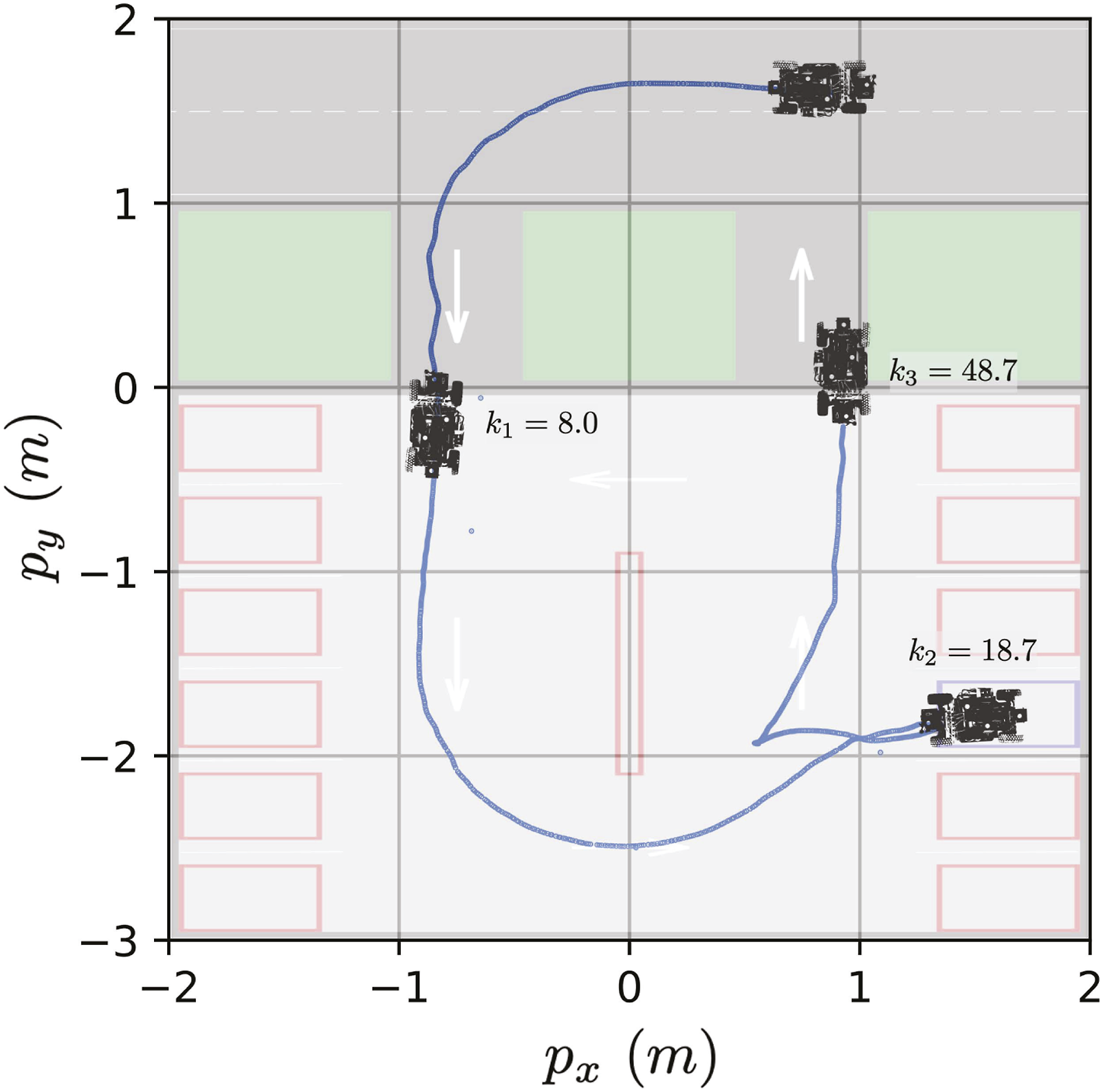
For our evaluation, we initialize the SVEA vehicle with the initial state of x
0
= [1, 1.75, − π, 0]. At this initial state, φ
3
is robustly satisfiable. Figure 21 shows the position trajectory, where one can see that the specification is fulfilled. In Figure 22, we show the control input trajectories for acceleration and steering. We use k
1
, k
2
, k
3
to denote the minimal time instants that the automated vehicle reaches sets The position trajectory of a SVEA vehicle performing the parking task φ
parking
. The velocity and heading trajectories in response to the acceleration and steering inputs throughout the parking task φ
parking
.
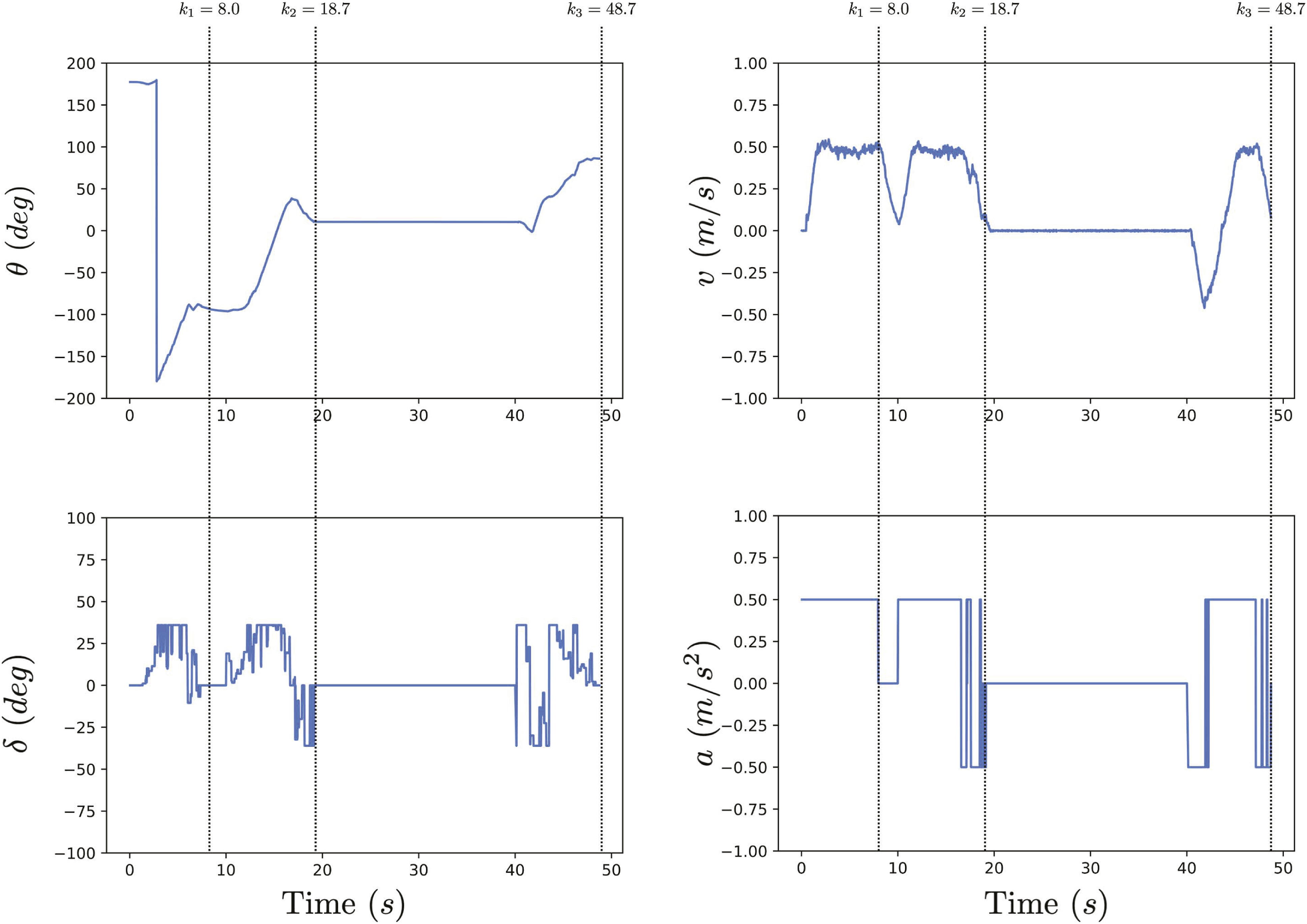
Finally, we report the computation time of this example, which was run in Matlab R2022b with the Level Set Method Toolbox (Mitchell and Templeton, 2005). We perform reachability analysis for constructing the tTLT offline on a Dell laptop with Ubuntu 20.04, Intel i7-4600U CPU 2.10 GHz and 8.0 GB RAM, which takes 2371.81 s. We note that the offline computation time for constructing the tTLT can be significantly reduced by using the python implementation (Bui et al., 2022). Throughout the parking task, we perform the online control synthesis on an NVIDIA Jetson TX2 embedded computer onboard the SVEA vehicle. The average time step of the online control synthesis is 0.001 s. A video demonstration of this experiment can be found at https://bit.ly/STL-TLT.
8. Conclusion
A novel approach for the online control synthesis of uncertain discrete-time systems under STL specifications was proposed in this paper. First, a real-time version of STL semantics and a notion of tTLT were introduced. Then the formal semantic connection between an STL formula and its corresponding tTLT was derived, i.e., a trajectory satisfying a tTLT also satisfies the corresponding STL formula. Finally, an online control synthesis algorithm was designed for the uncertain systems based on the connection between STL and tTLT. For the fragment of STL formulas under consideration, the soundness of the algorithm was proven. In the future, the control synthesis for multi-agent systems under local and/or global STL specifications is of interest.
Footnotes
Declaration of conflicting interests
The author(s) declared no potential conflicts of interest with respect to the research, authorship, and/or publication of this article.
Funding
The author(s) disclosed receipt of the following financial support for the research, authorship, and/or publication of this article: This work was supported by the Vetenskapsrådet (Distinguished Professor Grant 2017-01078 and International Postdoc Grant 2021-06727), Knut and Alice Wallenberg Foundation (Wallenberg Scholar Grant and Wallenberg Academy Fellow), the ERC COG LEAFHOUND (Grant agreement ID: 864720), and the ERC ADG FUN2MODEL (Grant agreement ID: 834115) and H2020 European Research Council under grant CoG LEAFHOUND.