The “Fluid Jacobian”: Modeling force-motion relationships in fluid-driven soft robots

Abstract

In this paper, we introduce the concept of the Fluid Jacobian, which provides a description of the power transmission that operates between the fluid and mechanical domains in soft robotic systems. It can be understood as a generalization of the traditional kinematic Jacobian that relates the joint space torques and velocities to the task space forces and velocities of a robot. In a similar way, the Fluid Jacobian relates fluid pressure to task space forces and fluid flow to task space velocities. In addition, the Fluid Jacobian can also be regarded as a generalization of the piston cross-sectional area in a fluid-driven cylinder that extends to complex geometries and multiple dimensions. In the following, we present a theoretical derivation of this framework, focus on important special cases, and illustrate the meaning and practical applicability of the Fluid Jacobian in four brief examples.

1. Introduction

Soft robots are commonly driven using hydraulic or pneumatic pressure (or vacuum). Such fluid powered soft systems employ a variety of actuator types such as bellows Pridham (1967), McKibben muscles Tondu (2012), and pneu-nets Mosadegh et al. (2014), and they come in a large range of designs including grippers Ilievski et al. (2011), crawlers Tolley et al. (2014), and swimmers Marchese et al. (2014). An important characteristic of soft robots is that the mechanical structure, the actuation, and other components are often indistinguishably connected and embedded in the same substrate. With this in mind, we will use the word actuator quite broadly when we talk about soft robotic systems in the following.

An important question in the context of such fluid-driven systems is how the pressure p in the fluid domain relates to the forces and torques F exerted in the mechanical domain, and how that relationship depends on the configuration q . That is, we are looking for an expression of the relationship

$\mathit{F}=f\left(\mathit{p},\mathit{q}\right),$

(1)

which is of high utility both in the control and the design of soft robotic systems. In conventional rigid robots, there exists a linear relationship between the forces in the actuator space (often referred to as the joint torques) and the forces in the task space. The inverse-transpose of the Jacobian of the mapping between these two spaces maps the joint torques to the task space forces (Siciliano et al. 2008, Chapter 3.3).

For fluid-driven soft robotic systems, deriving such a model is a much more challenging task, and the precise structure of equation (1) is not immediately apparent. Since mechanical structure and actuation are intertwined, the actuator space may not be well defined for many soft robotic systems. In addition, soft systems may have complex geometries, the actuators themselves may be elastically deformable, and additional reinforcing elements such as fibers, plates, or membranes contribute kinematic constraints and interrelate forces. Furthermore, many soft robotic systems are under actuated and the motion of the internal degrees of freedom is determined by an equilibrium between pressure-generated forces and elastic deformations. These effects are similar to under actuation in rigid robotic systems, such as robotic hands Birglen et al. (2007).

While in traditional hydraulics and pneumatics, the force exerted by a piston is simply the pressure multiplied by the area of the piston cross-section Ilango and Soundararajan (2011), we would expect a more complex, state-dependent, and potentially multidimensional relationship in soft robots. Only for very simple systems can solutions be derived by setting up expressions for the effective cross-sections while taking into account the forces exerted by the reinforcing elements Bruder et al. (2017); Habibian et al. (2022). For more complex systems, popular choices include formulations based on continuum mechanics models Sedal et al. (2017, 2018), often analyzed using finite element methods Buffinton et al. (2020); Xavier et al. (2021). As an alternative, learned models, for example, based on artificial neural networks Satheeshbabu et al. (2019); Hyatt et al. (2019); Thuruthel et al. (2018) or using Koopman operator theory Bruder et al. (2018a); Bruder et al. (2020); Bruder et al. (2021); Castaño et al. (2020); Haggerty et al. (2020), have been used for control. All these approaches, however, have in common that the resulting formulations can become quite complex and difficult to interpret. Most importantly, they do not reveal meaningful insights into the fundamental structure of equation (1).

In this paper, we introduce the concept of the Fluid Jacobian, which is an important characteristic of soft fluidic actuators, describing the relationship between pressure and force. More precisely, it provides a description of the power transmission between the fluid and the mechanical domains. It thus can be regarded as a generalization of the traditional kinematic Jacobian that relates joint torques and velocities to task space forces and velocities in a conventional robot. In a similar way, the Fluid Jacobian relates fluid pressure to task space forces and—as a dual—the change of fluid volume to task space velocities. In addition, the Fluid Jacobian can be regarded as a generalization of the piston cross-sectional area in a fluid-driven cylinder that extends to complex geometries and multiple dimensions.

In contrast to the models discussed in the above paragraph, our modeling approach is energy-based and our derivation of the Fluid Jacobian is based on a virtual power formulation, similar to the approach presented in Bishop-Moser et al. (2013). In this approach, the Fluid Jacobian of an actuator arises as the partial derivative of the fluid volume with respect to the task space variables, analogous to how traditional kinematic Jacobians are defined. The Fluid Jacobian has already been mentioned and employed in the modeling studies of Bruder et al. (2018b); Bruder and Wood (2021), and Sedal et al. (2021). A similar expression can be found in Pagitz et al. (2012) and Stölzle and Santina (2022). Here, we provide a detailed derivation and discussion that also treats elastic deformations, internal degrees of freedom, additional kinematic constraints, and experimental determination of the Fluid Jacobian.

In Section 2 of this paper, we first provide a theoretical derivation of the Fluid Jacobian for the most general case of a multi-cell soft actuator system which is subject to elastic deformation and additional kinematic constraints. To this end, a fluid space, a task space, and an internal motion space are introduced and connected via the appropriate Jacobians. A virtual power law is then used to establish force balances in the task space and internal motion space, respectively. We then consider a number of special cases and simplifications that have important applications in actual soft robotic systems. Through a number of examples of different soft robotic actuators, the application of the theory is illustrated in Section 3. Finally, we provide a detailed discussion of the Fluid Jacobian, its properties, and possible extensions in Section 4.

2. Derivation of the fluid Jacobian

2.1 Preliminaries

We assume that the configuration of a soft actuator system with n_v fluid-driven actuator units can be described by a vector q that lies in the system’s configuration space $\mathcal{C}\subset {\mathbb{R}}^{n_{\mathrm{q}}}$ . The number of configuration variables n_q can be quite large, and given the continuum nature of many soft actuators, $\mathcal{C}$ may have to be a suitable approximation of an infinite dimensional space.

Three important functions are defined over $\mathcal{C}$ :

1. The “useful” part of the motion of the soft robot is described by a holonomic forward kinematics function $\mathit{x}=\mathit{f}\left(\mathit{q}\right)$ , where $\mathit{x}\in {\mathbb{R}}^{n_{\mathrm{x}}}$ lies in the n_x-dimensional actuator task space. This task space may constitute a joint angle that is driven by the soft actuator, a multidimensional displacement that is created by a soft limb (e.g., described via a piecewise constant curvature model Della Santina et al. (2020)), or it could describe the closure of a soft gripper around an object. The kinematics function $\mathit{f}:\mathcal{C}\to {\mathbb{R}}^{n_{\mathrm{x}}}$ is assumed to be differentiable with respect to q , with the kinematic Jacobian ${\mathit{J}}_{\mathrm{x}}\left(\mathit{q}\right)\in {\mathbb{R}}^{n_{\mathrm{x}}\times n_{\mathrm{q}}}$ being defined as ${\mathit{J}}_{\mathrm{x}}:=\partial \mathit{f}\left(\mathit{q}\right)/\partial \mathit{q}$ . We further assume that the actuator system is not driven near a kinematic singularity; that is, the kinematic Jacobian has a full row rank of n_x. The forces and torques that the actuator applies within the task space are expressed by the vector $\mathit{F}\in {\mathbb{R}}^{n_{\mathrm{x}}}$ .

2. The internal volumes of the individual actuator units are expressed in a vector $\mathit{V}\in {\mathbb{R}}^{n_{\mathrm{v}}}$ . These volumes V may be expressed in terms of the configuration q through the function $\mathit{v}:\mathcal{C}\to {\mathbb{R}}^{n_{\mathrm{v}}}$ , as in $\mathit{V}=\mathit{v}\left(\mathit{q}\right)$ . Assuming that v is differentiable with respect to q , we define the volume Jacobian ${\mathit{J}}_{\mathrm{v}}\left(\mathit{q}\right)\in {\mathbb{R}}^{n_{\mathrm{v}}\times n_{\mathrm{q}}}$ as ${\mathit{J}}_{\mathrm{v}}:=\partial \mathit{v}\left(\mathit{q}\right)/\partial \mathit{q}$ . Each individual actuator unit, that is, each individual volume, may be pressurized to a different value and these pressures are expressed in the vector $\mathit{p}\in {\mathbb{R}}^{n_{\mathrm{v}}}$ .

3. The overall elastic energy E stored in the deformable structure of the actuator system may be expressed in terms of the configuration q through the elastic potential function $e:\mathcal{C}\to \mathbb{R}$ , as in $E=e\left(\mathit{q}\right)$ . This elastic potential leads to the restoring forces and torques ${\mathit{\tau }}_{\mathrm{E}}\left(\mathit{q}\right)=-{\left(\partial e\left(\mathit{q}\right)/\partial \mathit{q}\right)}^{\mathrm{T}}\in {\mathbb{R}}^{n_{\mathrm{q}}}$ .

Another important space that is implicitly defined via the function f is the null space of J _x. It characterizes the directions of actuator motions $\stackrel{.}{\mathit{q}}$ that do not create a task space motion $\stackrel{.}{\mathit{x}}$ . Locally, this null space is spanned by the rows of the orthogonal complement matrix ${\mathit{J}}_{\mathrm{y}}\in {\mathbb{R}}^{n_{\mathrm{y}}\times n_{\mathrm{q}}}$ , with ${\mathit{J}}_{\mathrm{x}}{\mathit{J}}_{\mathrm{y}}^{\mathrm{T}}=\mathbf{0}$ . ¹ Consequently, the columns of J _y span the internal motion space of the soft actuator system. Since J _x is assumed to have full row rank, the dimension n_y of this internal motion space is given by n_y = n_q − n_x. Furthermore, the right Moore–Penrose inverses ${\mathit{J}}_{\mathrm{x}}^{+}={\mathit{J}}_{\mathrm{x}}^{\mathrm{T}}{\left({\mathit{J}}_{\mathrm{x}}{\mathit{J}}_{\mathrm{x}}^{\mathrm{T}}\right)}^{-1}$ and ${\mathit{J}}_{\mathrm{y}}^{+}={\mathit{J}}_{\mathrm{y}}^{\mathrm{T}}{\left({\mathit{J}}_{\mathrm{y}}{\mathit{J}}_{\mathrm{y}}^{\mathrm{T}}\right)}^{-1}$ are well defined, and it holds that $\left[\begin{array}{l}{\mathit{J}}_{\mathrm{x}}\\ {\mathit{J}}_{\mathrm{y}}\end{array}\right]\left[\begin{array}{ll}{\mathit{J}}_{\mathrm{x}}^{+}& {\mathit{J}}_{\mathrm{y}}^{+}\end{array}\right]=\mathbf{1}$ . In other words, the mapping from the configuration space to the task and internal motion space is locally invertible with an inverse function $\mathit{q}={\mathit{f}}_{\text{local}}^{-1}\left(\mathit{x},\mathit{y}\right)$ and the associated Jacobians ${\mathit{J}}_{\mathrm{x}}^{+}$ and ${\mathit{J}}_{\mathrm{y}}^{+}$ . Note that due to the common nonlinearities, including contact, that occur in soft robot structures these mappings might only be established locally. Furthermore, due to the ambiguities in the definition of J _y as an orthogonal complement, the exact choice of the coordinates y that span the space of internal motion is not uniquely defined. That is, there exists infinitely many ${\mathit{J}}_{\mathrm{y}}\in {\mathbb{R}}^{n_{\mathrm{y}}\times n_{\mathrm{q}}}$ which fulfill the condition ${\mathit{J}}_{\mathrm{x}}{\mathit{J}}_{\mathrm{y}}^{\mathrm{T}}=\mathbf{0}$ , including every transformed Jacobian ${\mathit{J}}_{\overline{\mathrm{y}}}=\mathit{A}{\mathit{J}}_{\mathrm{y}}$ based on an arbitrary transformation matrix $\mathit{A}\in {\mathbb{R}}^{n_{\mathrm{y}}\times n_{\mathrm{y}}}$ , since ${\mathit{J}}_{\mathrm{x}}{\mathit{J}}_{\overline{\mathrm{y}}}^{\mathrm{T}}={\mathit{J}}_{\mathrm{x}}{\mathit{J}}_{\mathrm{y}}^{\mathrm{T}}{\mathit{A}}^{\mathrm{T}}=\mathbf{0}{\mathit{A}}^{\mathrm{T}}=\mathbf{0}$ .

2.2 Force balance

To establish a relationship between the action of the actuator (expressed via the vector F ) and the applied pressures (expressed via the vector p ), we provide an expression for the virtual power performed on the actuator by the fluid pressures, the elastic potential, and the reaction to the task space forces:

$\delta P=\delta {\stackrel{.}{\mathit{V}}}^{\mathrm{T}}\mathit{p}+\delta {\stackrel{.}{\mathit{q}}}^{\mathrm{T}}{\mathit{\tau }}_{\mathrm{E}}-\delta {\stackrel{.}{\mathit{x}}}^{\mathrm{T}}\mathit{F}.$

(2)

Note the minus sign in front of F is a result of F being defined as the force that the actuator applies onto the environment. From the kinematics introduced above, we obtain the following relationships for the virtual velocities: $\delta \stackrel{.}{\mathit{x}}={\mathit{J}}_{\mathrm{x}}\delta \stackrel{.}{\mathit{q}}$ and $\delta \stackrel{.}{\mathit{V}}={\mathit{J}}_{\mathrm{v}}\delta \stackrel{.}{\mathit{q}}$ . These lead to:

$\delta P=\delta {\stackrel{.}{\mathit{q}}}^{\mathrm{T}}{\mathit{J}}_{\mathrm{v}}^{\mathrm{T}}\mathit{p}+\delta {\stackrel{.}{\mathit{q}}}^{\mathrm{T}}{\mathit{\tau }}_{\mathrm{E}}-\delta {\stackrel{.}{\mathit{q}}}^{\mathrm{T}}{\mathit{J}}_{\mathrm{x}}^{\mathrm{T}}\mathit{F}.$

(3)

As the virtual work vanishes for all $\delta \stackrel{.}{\mathit{q}}$ , we arrive at the following balance of forces in the configuration space:

${\mathit{J}}_{\mathrm{v}}^{\mathrm{T}}\mathit{p}+{\mathit{\tau }}_{\mathrm{E}}-{\mathit{J}}_{\mathrm{x}}^{\mathrm{T}}\mathit{F}=\mathbf{0}$

(4)

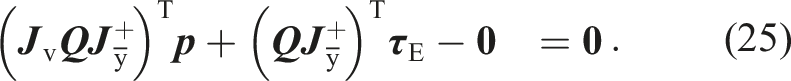
We can further simplify this equation by projecting into the task space and the internal motion space, respectively (Blajer, 2001). This projection is achieved by multiplying from the left with ${\left[\begin{array}{ll}{\mathit{J}}_{\mathrm{x}}^{+}& {\mathit{J}}_{\mathrm{y}}^{+}\end{array}\right]}^{\mathrm{T}}$ . With ${\mathit{J}}_{\mathrm{x}}{\mathit{J}}_{\mathrm{x}}^{+}=\mathbf{1}$ and ${\mathit{J}}_{\mathrm{x}}{\mathit{J}}_{\mathrm{y}}^{+}=\mathbf{0}$ , this leads to the following two equations:

$\begin{array}{ll}{\left({\mathit{J}}_{\mathrm{v}}{\mathit{J}}_{\mathrm{x}}^{+}\right)}^{\mathrm{T}}\mathit{p}+{\left({\mathit{J}}_{\mathrm{x}}^{+}\right)}^{\mathrm{T}}{\mathit{\tau }}_{\mathrm{E}}-\mathit{F}& =\mathbf{0}\end{array}$

(5)

$\begin{array}{ll}{\left({\mathit{J}}_{\mathrm{v}}{\mathit{J}}_{\mathrm{y}}^{+}\right)}^{\mathrm{T}}\mathit{p}+{\left({\mathit{J}}_{\mathrm{y}}^{+}\right)}^{\mathrm{T}}{\mathit{\tau }}_{\mathrm{E}}-\mathbf{0}& =\mathbf{0}\end{array}.$

(6)

We now define the Task Space Fluid Jacobian (or simply Fluid Jacobian) to be ${\mathit{J}}_{\mathrm{v},\mathrm{x}}:={\mathit{J}}_{\mathrm{v}}{\mathit{J}}_{\mathrm{x}}^{+}$ and the Internal Motion Fluid Jacobian to be ${\mathit{J}}_{\mathrm{v},\mathrm{y}}:={\mathit{J}}_{\mathrm{v}}{\mathit{J}}_{\mathrm{y}}^{+}$ . Furthermore, we introduce the abbreviations ${\mathit{\tau }}_{\mathrm{E},\mathrm{x}}:={\left({\mathit{J}}_{\mathrm{x}}^{+}\right)}^{\mathrm{T}}{\mathit{\tau }}_{\mathrm{E}}$ and ${\mathit{\tau }}_{\mathrm{E},\mathrm{y}}:={\left({\mathit{J}}_{\mathrm{y}}^{+}\right)}^{\mathrm{T}}{\mathit{\tau }}_{\mathrm{E}}$ . With these abbreviations, the final force balance has the form:

$\begin{array}{ll}\mathit{F}& ={\mathit{J}}_{\mathrm{v},\mathrm{x}}^{\mathrm{T}}\left(\mathit{q}\right)\mathit{p}+{\mathit{\tau }}_{\mathrm{E},\mathrm{x}}\left(\mathit{q}\right)\end{array}$

(7)

$\begin{array}{ll}\mathbf{0}& ={\mathit{J}}_{\mathrm{v},\mathrm{y}}^{\mathrm{T}}\left(\mathit{q}\right)\mathit{p}+{\mathit{\tau }}_{\mathrm{E},\mathrm{y}}\left(\mathit{q}\right)\end{array}.$

(8)

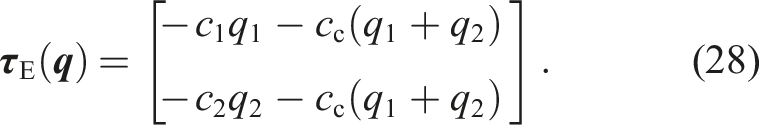
The first of these two equations describes the force balance in task space: forces F are balanced by the pressure in the actuator p and the elastic deformation τ _E,x. Since the task space is well-defined, this expression is unique. The second equation is the force balance in the internal motion space. It describes the elastic deformation of the internal degrees of freedom of the actuator in reaction to the applied pressure in the actuator. The actuator pressure p enters both equations linearly by means of the Fluid Jacobians. In the most general case, however, there is a nonlinear mapping between pressure p and task space forces F , as the two equations are coupled through the overall configuration q . That is, a change in pressure leads to a change in the internal deformation via equation (8), which influences the Fluid Jacobian and elastic forces in equation (7).

2.3 Simplifications and special cases

2.3.1 No internal motion

An important special case is a soft actuator system without internal degrees of freedom. For many soft robotic systems, this holds at least approximately, as parasitic internal motion is undesired and thus often avoided by design. For example, in bellow-like actuators Pridham (1967); Usevitch et al. (2018); Han et al. (2018), origami actuators Kim and Gillespie (2015); Zaghloul and Bone (2023), or in fiber sleeve actuators Ball et al. (2016); Bishop-Moser and Kota (2015). Mathematically, in this case the task and configuration spaces are identical. Consequently, it holds that J _x = 1, and thus J _v,x = J _v and τ _E,x = τ _E. The matrix J _y and equation (8) vanish. Equation (7) then simplifies to:

$\mathit{F}={\mathit{J}}_{\mathrm{v}}^{\mathrm{T}}\left(\mathit{q}\right)\mathit{p}+{\mathit{\tau }}_{\mathrm{E}}\left(\mathit{q}\right).$

(9)

This simplified form of the force balance has already been reported in Bruder et al. (2018b) and Sedal et al. (2021). In these publications, the elastic forces were further approximated with a linear elasticity model: τ _E = − K Δ q . Since there are no coupling effects, the task space forces F are linear in pressure, and the Fluid Jacobian represents a generalization of the piston area of a traditional hydraulic or pneumatic cylinder.

2.3.2 Explicit internal motion space

As a second special case, we consider actuator systems in which a description of the internal deformation y can be defined explicitly and a global inverse mapping $\mathit{q}={\mathit{f}}_{\text{glob}}^{-1}\left(\mathit{x},\mathit{y}\right)$ exists. In this case, we can express the volume V and elastic energy E as a function of x and y , and we can thus compute ${\mathit{J}}_{\mathrm{x}}^{+}$ , ${\mathit{J}}_{\mathrm{y}}^{+}$ , J _v,x, J _v,y, τ _E,x, and τ _E,y explicitly as partial derivatives of ${\mathit{f}}_{\text{glob}}^{-1}\left(\right)$ , $\mathit{v}\left(\right)$ , and $e\left(\right)$ :

$\begin{array}{llll}{\mathit{J}}_{\mathrm{x}}^{+}& =\frac{\partial {\mathit{f}}_{\text{glob}}^{-1}\left(\mathit{x},\mathit{y}\right)}{\partial \mathit{x}}& {\mathit{J}}_{\mathrm{y}}^{+}& =\frac{\partial {\mathit{f}}_{\text{glob}}^{-1}\left(\mathit{x},\mathit{y}\right)}{\partial \mathit{y}}\\ {\mathit{J}}_{\mathrm{v},\mathrm{x}}& =\frac{\partial \mathit{v}\left(\mathit{x},\mathit{y}\right)}{\partial \mathit{x}}& {\mathit{J}}_{\mathrm{v},\mathrm{y}}& =\frac{\partial \mathit{v}\left(\mathit{x},\mathit{y}\right)}{\partial \mathit{y}}\\ {\mathit{\tau }}_{\mathrm{E},\mathrm{x}}& =-{\left(\frac{\partial e\left(\mathit{x},\mathit{y}\right)}{\partial \mathit{x}}\right)}^{\mathrm{T}}& {\mathit{\tau }}_{\mathrm{E},\mathrm{y}}& =-{\left(\frac{\partial e\left(\mathit{x},\mathit{y}\right)}{\partial \mathit{y}}\right)}^{\mathrm{T}}\end{array}$

(10)

Let us now first examine the additional simplification of τ _E = 0. That is, of a soft actuator without elastic energy storage. This could be an origami-type system Kim and Gillespie (2015), or a bladder-like actuator made from thin but inextensible material Niiyama et al. (2014); Greer et al. (2017); Bruder and Wood (2021). Without elastic forces, equation (8) reduces to:

${\mathit{J}}_{\mathrm{v},\mathrm{y}}^{\mathrm{T}}\left(\mathit{x},\mathit{y}\right)\mathit{p}=\mathbf{0}.$

(11)

For nonzero pressures, this can only hold if ${\mathit{J}}_{\mathrm{v},\mathrm{y}}^{\mathrm{T}}$ vanishes; that is, if the volume function $\mathit{v}\left(\mathit{x},\mathit{y}\right)$ becomes extremal with respect to the internal motion y . For positive pressures, this extremum corresponds to a configuration that maximizes the volume of each actuator unit; for vacuum-driven systems, the volumes would be minimized. As long as ${\partial }^2\mathit{v}\left(\mathit{x},\mathit{y}\right)/\partial {\mathit{y}}^2$ is nonzero, the implicit equation ${\mathit{J}}_{\mathrm{v},\mathrm{y}}^{\mathrm{T}}\left(\mathit{x},\mathit{y}\right)=0$ can be inverted, such that y can be expressed as a function of x as in $\mathit{y}=\mathit{y}\left(\mathit{x}\right)$ . Physically, this nonzero-condition means that the volume has a maximal/minimal value; that is, it is mechanically bounded ² . In other words, the internal motion of such an actuator system is fully defined by the task space motion and independent of pressure. Equation (7) thus becomes:

$\mathit{F}={\mathit{J}}_{\mathrm{v},\mathrm{x}}^{\mathrm{T}}\left(\mathit{x},\mathit{y}\left(\mathit{x}\right)\right)\mathit{p}={\mathit{J}}_{\mathrm{v},\mathrm{x}}^{\mathrm{T}}\left(\mathit{x}\right)\mathit{p}$

(12)

which is, again, linear in pressure p .

This linearity is lost, as soon as we include elastic deformations of the actuator. In this case equation (8) remains mostly unchanged and is only restated with x and y as arguments:

${\mathit{J}}_{\mathrm{v},\mathrm{y}}^{\mathrm{T}}\left(\mathit{x},\mathit{y}\right)\mathit{p}+{\mathit{\tau }}_{\mathrm{E},\mathrm{y}}\left(\mathit{x},\mathit{y}\right)=\mathbf{0}.$

(13)

This equation provides an implicit relationship between x , y , and p , which can be solved for y = y ( x , p ), as long as ${\partial }^2\mathit{v}\left(\mathit{x},\mathit{y}\right)/\partial {\mathit{y}}^2+{\partial }^{2}e\left(\mathit{x},\mathit{y}\right)/\partial {\mathit{y}}^2\ne \mathbf{0}$ . That is, as long as the internal motion is bounded either by a maximal/minimal volume or through elastic forces. Substituting this expression for y into equation (7) yields:

$\mathit{F}={\mathit{J}}_{\mathrm{v},\mathrm{x}}^{\mathrm{T}}\left(\mathit{x},\mathit{p}\right)\mathit{p}+{\mathit{\tau }}_{\mathrm{E},\mathrm{y}}\left(\mathit{x},\mathit{p}\right).$

(14)

We can see that this relationship is no longer linear in p , as changes in pressure now influence the internal deformation, which—in turn—affects the elastic force in the task space and alters the task space Fluid Jacobian.

The opening premise of this section was that the internal deformation y can be defined explicitly and that a global mapping $\mathit{q}={\mathit{f}}_{\text{glob}}^{-1}\left(\mathit{x},\mathit{y}\right)$ exists. This is, of course, only necessary if we seek to derive the Jacobians in equation (10) analytically. Physically, these relationships still hold, even if we do not have an explicit description of y or if the internal motions space becomes infinite dimensional.

2.3.3 Linearized Equations

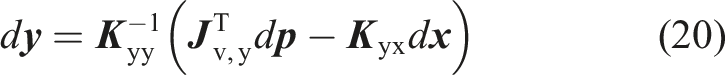
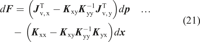
The influence of the internal motion on the task space forces that was described in the previous section can be examined further by considering a linearization of equations (7) and (8). To this end, we take the total differential, leading to:

$\begin{array}{ll}d\mathit{F}& =\frac{\partial {\mathit{J}}_{\mathrm{v},\mathrm{x}}^{\mathrm{T}}\mathit{p}}{\partial \mathit{q}}d\mathit{q}+{\mathit{J}}_{\mathrm{v},\mathrm{x}}^{\mathrm{T}}d\mathit{p}+\frac{\partial {\mathit{\tau }}_{\mathrm{E},\mathrm{x}}}{\partial \mathit{q}}d\mathit{q}\end{array}$

(15)

$\begin{array}{ll}\mathbf{0}& =\frac{\partial {\mathit{J}}_{\mathrm{v},\mathrm{y}}^{\mathrm{T}}\mathit{p}}{\partial \mathit{q}}d\mathit{q}+{\mathit{J}}_{\mathrm{v},\mathrm{x}}^{\mathrm{T}}d\mathit{p}+\frac{\partial {\mathit{\tau }}_{\mathrm{E},\mathrm{y}}}{\partial \mathit{q}}d\mathit{q}\end{array}$

(16)

After substituting $d\mathit{q}={\mathit{J}}_{\mathrm{x}}^{+}d\mathit{x}+{\mathit{J}}_{\mathrm{y}}^{+}d\mathit{y}$ , we get:

$\begin{array}{ll}d\mathit{F}& ={\mathit{J}}_{\mathrm{v},\mathrm{x}}^{\mathrm{T}}d\mathit{p}-{\mathit{K}}_{\text{xx}}d\mathit{x}-{\mathit{K}}_{\text{xy}}d\mathit{y}\end{array}$

(17)

$\begin{array}{ll}\mathbf{0}& ={\mathit{J}}_{\mathrm{v},\mathrm{y}}^{\mathrm{T}}d\mathit{p}-{\mathit{K}}_{\text{yx}}d\mathit{x}-{\mathit{K}}_{\text{yy}}d\mathit{y}\end{array}$

(18)

with ³

$\begin{array}{ll}{\mathit{K}}_{\text{xx}}& =-\frac{\partial {\mathit{J}}_{\mathrm{v},\mathrm{x}}^{\mathrm{T}}\mathit{p}}{\partial \mathit{q}}{\mathit{J}}_{\mathrm{x}}^{+}-\frac{\partial {\mathit{\tau }}_{\mathrm{E},\mathrm{x}}}{\partial \mathit{q}}{\mathit{J}}_{\mathrm{x}}^{+}\\ {\mathit{K}}_{\text{xy}}& =-\frac{\partial {\mathit{J}}_{\mathrm{v},\mathrm{x}}^{\mathrm{T}}\mathit{p}}{\partial \mathit{q}}{\mathit{J}}_{\mathrm{y}}^{+}-\frac{\partial {\mathit{\tau }}_{\mathrm{E},\mathrm{x}}}{\partial \mathit{q}}{\mathit{J}}_{\mathrm{y}}^{+}\\ {\mathit{K}}_{\text{yx}}& =-\frac{\partial {\mathit{J}}_{\mathrm{v},\mathrm{y}}^{\mathrm{T}}\mathit{p}}{\partial \mathit{q}}{\mathit{J}}_{\mathrm{x}}^{+}-\frac{\partial {\mathit{\tau }}_{\mathrm{E},\mathrm{y}}}{\partial \mathit{q}}{\mathit{J}}_{\mathrm{x}}^{+}\\ {\mathit{K}}_{\text{yy}}& =-\frac{\partial {\mathit{J}}_{\mathrm{v},\mathrm{y}}^{\mathrm{T}}\mathit{p}}{\partial \mathit{q}}{\mathit{J}}_{\mathrm{y}}^{+}-\frac{\partial {\mathit{\tau }}_{\mathrm{E},\mathrm{y}}}{\partial \mathit{q}}{\mathit{J}}_{\mathrm{y}}^{+}\end{array}$

(19)

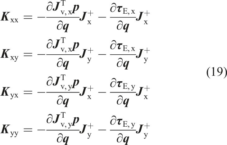
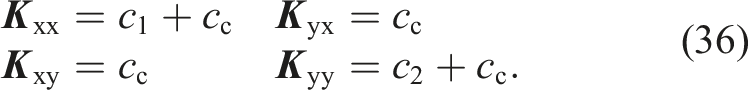
These terms represent equivalent stiffness matrices with physical units of force/torque per unit translational/angular displacement. They relate motion in the task space and the internal motion spaces to the resulting generalized forces. In particular, K _xx is the stiffness of the task space which acts in parallel to the motion of the output, K _yy is the stiffness of the internal motion space which acts in series to the output, and K _xy/ K _yx couple the two spaces. The generalized forces arise not only from elastic deformations due to τ _E, but also result from changes to the fluid Jacobian and the consequent modifications in the conversion of pressures into generalized forces. Using these stiffnesses to resolve the internal motion, we obtain:

$d\mathit{y}={\mathit{K}}_{\text{yy}}^{-1}\left({\mathit{J}}_{\mathrm{v},\mathrm{y}}^{\mathrm{T}}d\mathit{p}-{\mathit{K}}_{\text{yx}}d\mathit{x}\right)$

(20)

and hence:

$\begin{array}{l}d\mathit{F}=\left({\mathit{J}}_{\mathrm{v},\mathrm{x}}^{\mathrm{T}}-{\mathit{K}}_{\text{xy}}{\mathit{K}}_{\text{yy}}^{-1}{\mathit{J}}_{\mathrm{v},\mathrm{y}}^{\mathrm{T}}\right)d\mathit{p}\hspace{1em}\dots \\ -\left({\mathit{K}}_{\text{xx}}-{\mathit{K}}_{\text{xy}}{\mathit{K}}_{\text{yy}}^{-1}{\mathit{K}}_{\text{yx}}\right)d\mathit{x}\end{array}$

(21)

Ignoring the influence of q on these stiffness matrices, we can approximate the change in energy that is stored in K _xx by dE_x = 1/2d x ^T K _xxd x and in the energy stored in K _yy by $d{E}_{\mathrm{y}}=1/2d{\mathit{y}}^{\mathrm{T}}{\mathit{K}}_{\text{yy}}d\mathit{y}=1/2{\left({\mathit{J}}_{\mathrm{v},\mathrm{y}}^{\mathrm{T}}d\mathit{p}-{\mathit{K}}_{\text{yx}}d\mathit{x}\right)}^{\mathrm{T}}{\mathit{K}}_{\text{yy}}^{-1}\left({\mathit{J}}_{\mathrm{v},\mathrm{y}}^{\mathrm{T}}d\mathit{p}-{\mathit{K}}_{\text{yx}}d\mathit{x}\right)$ . These equations highlight what is required to achieve as closely as possible an actuator that acts as an ideal transformer without parasitic energy storage: K _xx and K _yx need to be as small as possible while K _yy should be as large as possible.

2.3.4 Extension to systems with additional constraints

In some cases, it may be convenient to express the configuration q with a set of non-minimal coordinates and include additional kinematic constraints in the model. We can do so in the framework described above by including an additional projection step in our formulation. Let us assume that there will be n_c additional, linearly independent, holonomic constraints on the configuration, limiting the number of independent degrees of freedom n_i to n_i = n_q − n_c. These constraints can be expressed implicitly as $\mathit{g}\left(\mathit{q}\right)=\mathbf{0}$ , with the constraint function $\mathit{g}:\mathcal{C}\to {\mathbb{R}}^{n_{\mathrm{c}}}$ and the associated constraint forces $\mathit{\lambda }\in {\mathbb{R}}^{n_{\mathrm{c}}}$ . The function g is assumed to be differentiable, with the constraint Jacobian ${\mathit{J}}_{\mathrm{g}}\left(\mathit{q}\right)\in {\mathbb{R}}^{n_{\mathrm{c}}\times n_{\mathrm{q}}}$ defined as ${\mathit{J}}_{\mathrm{g}}:=\partial \mathit{g}\left(\mathit{q}\right)/\partial \mathit{q}$ .

Let ${\mathit{Q}}^{\mathrm{T}}\in {\mathbb{R}}^{n_{\mathrm{i}}\times n_{\mathrm{q}}}$ denote the orthogonal complement matrix of J _g. That is, ${\mathit{J}}_{\mathrm{g}}\mathit{Q}=\mathbf{0}\iff {\mathit{Q}}^{\mathrm{T}}{\mathit{J}}_{\mathrm{g}}^{\mathrm{T}}=\mathbf{0}$ . Note that, for a given J _g, the matrix Q is not unique. Its columns define the directions of all velocities that are admissible under the constraints of g and thus span a virtual subspace of admissible motion Hemami and Weimer (1981). The matrix Q can also be interpreted as the Jacobian of a locally defined function $\mathit{q}=\mathit{q}\left({\mathit{q}}_{\min }\right)$ that maps a suitable choice of minimal coordinates ${\mathit{q}}_{\min }\in {\mathbb{R}}^{n_{\mathrm{i}}}$ to the admissible generalized coordinates $\mathit{q}\in \mathcal{C}$ .

The product ${\mathit{J}}_{\overline{\mathrm{x}}}={\mathit{J}}_{\mathrm{x}}\mathit{Q}\in {\mathbb{R}}^{n_{\mathrm{x}}\times n_{\mathrm{i}}}$ consequently describes the directions of admissible task space motion. Here, we make the important additional assumption that the matrix ${\mathit{J}}_{\overline{\mathrm{x}}}$ is non-singular (i.e., that it has a full row rank of n_x). This assumption implies two properties. First, the additional constraints of g only affect the internal degrees of freedom of the soft actuator system, not its task space motion. This can be ensured by a suitable choice of the task space. Second, the soft actuator is operated outside a kinematic singularity of the constraints.

Similar to J _y, we introduce ${\mathit{J}}_{\overline{\mathrm{y}}}\in {\mathbb{R}}^{n_{\overline{\mathrm{y}}}\times n_{\mathrm{i}}}$ to be the orthogonal complement of ${\mathit{J}}_{\overline{\mathrm{x}}}$ , such that ${\mathit{J}}_{\overline{\mathrm{x}}}{\mathit{J}}_{\overline{\mathrm{y}}}^{\mathrm{T}}=\mathbf{0}$ . Since ${\mathit{J}}_{\overline{\mathrm{x}}}$ has full row rank, the dimension $n_{\overline{\mathrm{y}}}$ of these internal motions is given by $n_{\overline{\mathrm{y}}}=n_{\mathrm{i}}-n_{\mathrm{x}}$ .

The virtual power equation now also has to include a term for the virtual work performed by the constraints:

$\delta P=\delta {\stackrel{.}{\mathit{V}}}^{\mathrm{T}}\mathit{p}+\delta {\stackrel{.}{\mathit{c}}}^{\mathrm{T}}\mathit{\lambda }+\delta {\stackrel{.}{\mathit{q}}}^{\mathrm{T}}{\mathit{\tau }}_{\mathrm{E}}-\delta {\stackrel{.}{\mathit{x}}}^{\mathrm{T}}\mathit{F},$

(22)

and the associated virtual velocities are given by $\delta \stackrel{.}{\mathit{c}}={\mathit{J}}_{\mathrm{g}}\delta \stackrel{.}{\mathit{q}}$ . Dropping the δ q leads to:

${\mathit{J}}_{\mathrm{v}}^{\mathrm{T}}\mathit{p}+{\mathit{J}}_{\mathrm{g}}^{\mathrm{T}}\mathit{\lambda }+{\mathit{\tau }}_{\mathrm{E}}-{\mathit{J}}_{\mathrm{x}}^{\mathrm{T}}\mathit{F}=\mathbf{0}.$

(23)

In contrast to the formulation introduced above, we now have to perform two projections. The first projects into the space of admissible motions and the second into the task space and the space of internal motions, respectively. These projections are achieved by multiplying from the left with ${\left[\begin{array}{ll}{\mathit{J}}_{\overline{\mathrm{x}}}^{+}& {\mathit{J}}_{\overline{\mathrm{y}}}^{+}\end{array}\right]}^{\mathrm{T}}{\mathit{Q}}^{\mathrm{T}}$ . With ${\mathit{Q}}^{\mathrm{T}}{\mathit{J}}_{\mathrm{g}}^{\mathrm{T}}=\mathbf{0}$ , ${\mathit{Q}}^{\mathrm{T}}{\mathit{J}}_{\mathrm{x}}^{\mathrm{T}}={\left({\mathit{J}}_{\mathrm{x}}\mathit{Q}\right)}^{\mathrm{T}}={\mathit{J}}_{\overline{\mathrm{x}}}^{\mathrm{T}}$ , ${\mathit{J}}_{\overline{\mathrm{x}}}^{+}{\mathit{J}}_{\overline{\mathrm{x}}}=\mathbf{1}$ and ${\mathit{J}}_{\overline{\mathrm{x}}}{\mathit{J}}_{\overline{\mathrm{y}}}^{\mathrm{T}}=\mathbf{0}$ , this leads to two constraint-free equations:

$\begin{array}{ll}{\left({\mathit{J}}_{\mathrm{v}}\mathit{Q}{\mathit{J}}_{\overline{\mathrm{x}}}^{+}\right)}^{\mathrm{T}}\mathit{p}+{\left(\mathit{Q}{\mathit{J}}_{\overline{\mathrm{x}}}^{+}\right)}^{\mathrm{T}}{\mathit{\tau }}_{\mathrm{E}}-\mathit{F}& =\mathbf{0}\end{array}$

(24)

$\begin{array}{ll}{\left({\mathit{J}}_{\mathrm{v}}\mathit{Q}{\mathit{J}}_{\overline{\mathrm{y}}}^{+}\right)}^{\mathrm{T}}\mathit{p}+{\left(\mathit{Q}{\mathit{J}}_{\overline{\mathrm{y}}}^{+}\right)}^{\mathrm{T}}{\mathit{\tau }}_{\mathrm{E}}-\mathbf{0}& =\mathbf{0}\end{array}.$

(25)

and with the new abbreviations ( ${\mathit{J}}_{\mathrm{v},\mathrm{x}}:={\mathit{J}}_{\mathrm{v}}\mathit{Q}{\mathit{J}}_{\overline{\mathrm{x}}}^{+}$ , ${\mathit{J}}_{\mathrm{v},\mathrm{y}}:={\mathit{J}}_{\mathrm{v}}\mathit{Q}{\mathit{J}}_{\overline{\mathrm{y}}}^{+}$ , ${\mathit{\tau }}_{\mathrm{E},\mathrm{x}}:={\left(\mathit{Q}{\mathit{J}}_{\overline{\mathrm{x}}}^{+}\right)}^{\mathrm{T}}{\mathit{\tau }}_{\mathrm{E}}$ and ${\mathit{\tau }}_{\mathrm{E},\mathrm{y}}:={\left(\mathit{Q}{\mathit{J}}_{\overline{\mathrm{y}}}^{+}\right)}^{\mathrm{T}}{\mathit{\tau }}_{\mathrm{E}}$ ) we arrive at the same form as in equations (7) and (8).

3. Examples

In this section, we examine four examples of fluid-driven actuators. Our goal is two-fold. On the one hand, we seek to provide insight into the theoretical results presented in the previous section and to visualize the physical meaning of the derived equations. On the other hand, we want to show how the Fluid Jacobian can be obtained in practical examples and how it can be applied in real systems to predict forces as a function of pressure and state. As a consequence, the examples range from simplified/contrived and theoretical, to actual actuators that are physically built and experimentally examined.

3.1 Double cylinder

Our first example is not truly a soft actuator, but a contrived example of a double-acting cylinder with additional elastic elements. Its primary purpose is to highlight and visualize the terms that are found in equations (7) and (8) and to relate the concept of the Fluid Jacobian to the piston areas in traditional pneumatic and hydraulic cylinders. It consists of a single cylinder chamber (with pressure p) with two pistons acting in opposite directions (Figure 1). The positions of the two pistons are described by the configuration variables $\mathit{q}={\left[\begin{array}{ll}{q}_1& q_2\end{array}\right]}^T$ , and the piston areas are given as A₁ and A₂. Two springs (with stiffnesses c₁ and c₂) are mounted in parallel to the pistons, and a third spring (with stiffness c_c) links the motions of the two pistons. All springs are unloaded when q₁ = q₂ = 0. An external load (with task space position x and task space force F) acts directly on piston 1, while piston 2 is acted upon only by the two connected springs.

Figure 1.

Cylinder with elastic elements connecting two pistons acting in opposite directions.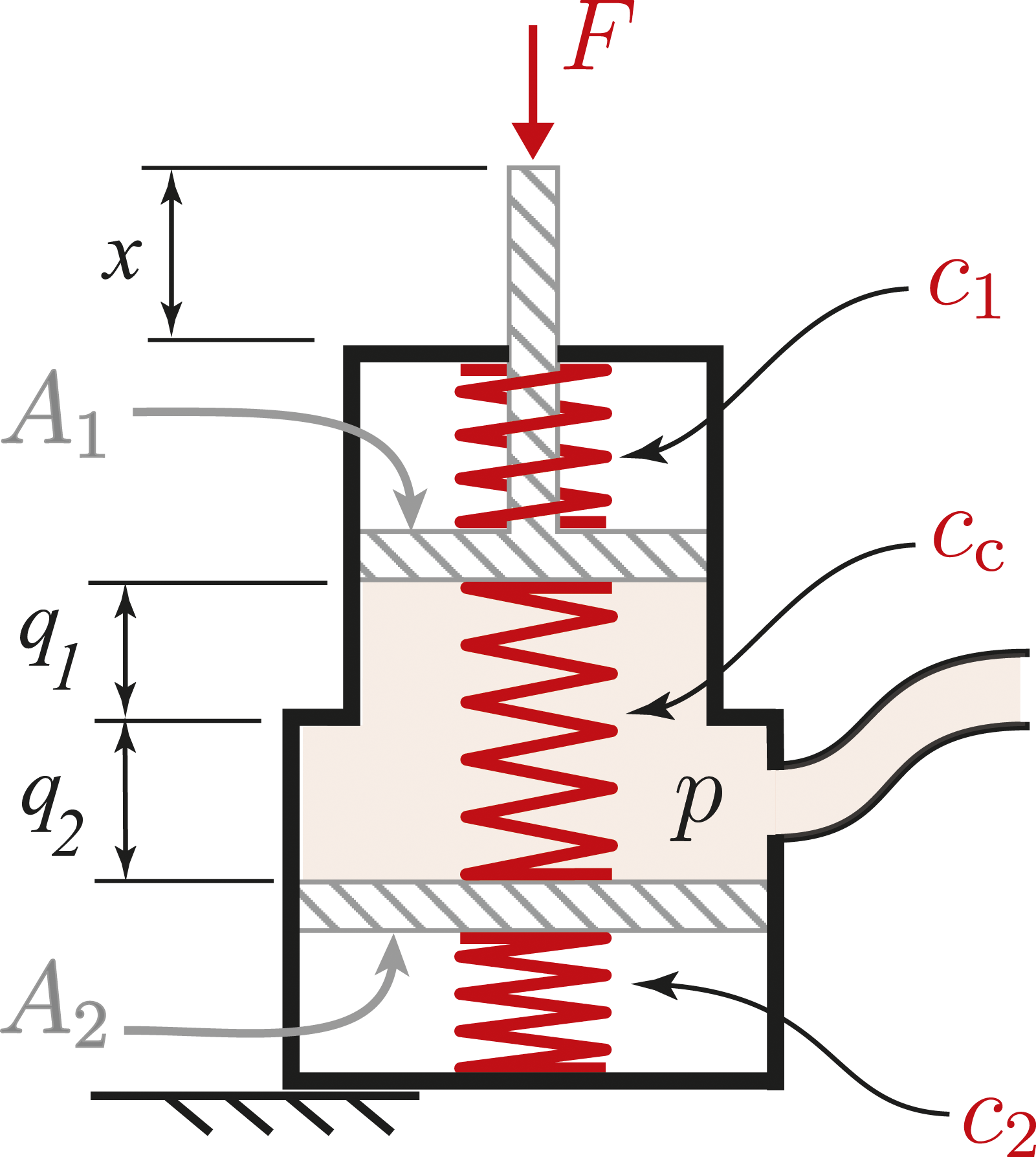

For this system, the forward kinematics are given as $x=\mathit{f}\left(\mathit{q}\right)=q_1$ , the internal volume is $V=\mathit{v}\left(\mathit{q}\right)=q_1{A}_1+q_2{A}_2$ , the elastic energy is $E=e\left(\mathit{q}\right)=\frac{1}{2}{c}_1{q}_1^2+\frac{1}{2}{c}_2{q}_2^2+\frac{1}{2}{c}_{\mathrm{c}}{\left(q_1+q_2\right)}^2$ , and there are no additional constraints. Hence:

$\begin{array}{ll}{\mathit{J}}_{\mathrm{x}}& =\left[\begin{array}{ll}1& 0\end{array}\right]\end{array}$

(26)

$\begin{array}{ll}{\mathit{J}}_{\mathrm{v}}& =\left[\begin{array}{ll}{A}_1& A_2\end{array}\right]\end{array}$

(27)

$\begin{array}{ll}{\mathit{\tau }}_{\mathrm{E}}\left(\mathit{q}\right)& =\left[\begin{array}{l}-c_1{q}_1-c_{\mathrm{c}}\left(q_1+q_2\right)\\ -c_2{q}_2-c_{\mathrm{c}}\left(q_1+q_2\right)\end{array}\right]\end{array}.$

(28)

Since there are no additional constraints, we can compute J _y as the orthogonal complement to J _x, which is ${\mathit{J}}_{\mathrm{y}}=\left[\begin{array}{ll}0& 1\end{array}\right]$ . With this, we get:

$\begin{array}{ll}{\mathit{J}}_{\mathrm{v},\mathrm{x}}& =A_1\end{array}$

(29)

$\begin{array}{ll}{\mathit{J}}_{\mathrm{v},\mathrm{y}}& =A_2\end{array}$

(30)

$\begin{array}{ll}{\mathit{\tau }}_{\mathrm{E},\mathrm{x}}& =-c_1{q}_1-c_{\mathrm{c}}\left(q_1+q_2\right)\end{array}$

(31)

$\begin{array}{ll}{\mathit{\tau }}_{\mathrm{E},\mathrm{y}}& =-c_2{q}_2-c_{\mathrm{c}}\left(q_1+q_2\right)\end{array}$

(32)

and thus:

$F=A_{1}p-\left(c_1+c_{\mathrm{c}}\right)q_1-c_{\mathrm{c}}{q}_2$

(33)

$0=A_{2}p-c_{\mathrm{c}}{q}_1-\left(c_{\mathrm{c}}+c_2\right)q_2.$

(34)

We can solve the second equation for the unactuated degree of freedom, q₂ and obtain for F:

$F=\left(A_1-\frac{c_{\mathrm{c}}}{c_{\mathrm{c}}+c_2}{A}_2\right)p-\left(c_1+\frac{c_{\mathrm{c}}{c}_2}{c_{\mathrm{c}}+c_2}\right)q_1.$

(35)

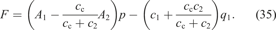
This example nicely illustrates the role of the different components of equations (7) and (8). The two Fluid Jacobians in equations (29) and (30) are equal to the cross-sectional areas of the pistons associated with internal and task space motion. In this special case, they do not depend on the state q . As can be seen in equation (35), the internal motion against A₂ still influences the force F in the task space. This is due to the elastic coupling between internal motion and the task space via the spring of stiffness c_c. In this example, the resulting equations are linear in both q _min and q , and the stiffness terms of (19) are:

$\begin{array}{llll}{\mathit{K}}_{\text{xx}}& =c_1+c_{\mathrm{c}}& {\mathit{K}}_{\text{yx}}& =c_{\mathrm{c}}\\ {\mathit{K}}_{\text{xy}}& =c_{\mathrm{c}}& {\mathit{K}}_{\text{yy}}& =c_2+c_{\mathrm{c}}.\end{array}$

(36)

This example also highlights the series/parallel nature of these elastic elements. This is particularly evident when setting c_c = 0 where only the spring c₁ is connected to the output, exerting forces that act in parallel to the motion in the x direction. To grasp the series behavior of c₂, let’s imagine using an incompressible ⁴ fluid and closing the fluid port. In a conventional hydraulic cylinder, this would completely block the motion of the output. In contrast, in our example, the output can still be moved. The displacement of the piston at the output results in a corresponding displacement of the piston attached to the spring c₂, leading to a rise in pressure p. The effect is equivalent to including a series elastic element in the output.

As discussed above, to achieve an ideal transformer, K _xx and K _yx should be as small as possible, while K _yy should be as large as possible. Applied to this example, c₁ and c_c should approach 0 and c₂ should approach ∞. In other words, one should remove the springs c₁ and c_c, and replace the spring c₂ with a rigid connection. As one might expect, these changes would result in a conventional hydraulic/pneumatic cylinder with no springs and a rigid floor.

3.2 Fiber-reinforced elastomeric enclosure

A fiber-reinforced elastomeric enclosure (FREE) Bishop-Moser and Kota (2015); Krishnan et al. (2015); Bishop-Moser et al. (2013); Singh and Krishnan (2020), also known as a fiber-reinforced soft actuator (FRSA) Galloway et al. (2013); Connolly et al. (2015, 2017), is an actuator that consists of a fluid-filled elastomeric tube wound with reinforcing fibers, patterned to yield a desired mode and direction of deformation upon pressurization. By changing the angles and arrangement of these fibers, a FREE can be customized to yield a large variety of desired deformations and forces Bishop-Moser and Kota (2015). Their customizability combined with their flexibility and cylindrical shape makes these actuators well suited for applications such as a pipe inspection Singh et al. (2019), catheter actuation Gilbertson et al. (2016), grasping Uppalapati and Krishnan (2018), and manipulation Grissom et al. (2006); Satheeshbabu et al. (2019, 2020).

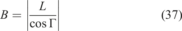
To make the computation of the Fluid Jacobian of a FREE tractable, we rely on a common assumption for FREES: that they maintain the geometry of an ideal cylinder Bishop-Moser and Kota (2015). This neglects the tapering of the actuator towards the end-caps, any potential bending along its main axis, and any bulging of the elastomeric tube between the fibers of the mesh.

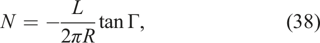
An ideal cylindrical FREE in its relaxed configuration (i.e., when fluid pressure is zero and no external loads are applied) can be described by a set of three parameters, L, R, and Γ, where L represents the relaxed length of the FREE, R represents the radius, and Γ the fiber angle (Figure 2(a)). For notational convenience, we further define:

$B=\left|\frac{L}{\cos \hspace{0.17em}\mathrm{\Gamma }}\right|$

(37)

$\begin{array}{ll}N& =-\frac{L}{2\pi R}\tan \hspace{0.17em}\mathrm{\Gamma }\end{array},$

(38)

where B is the length of one of the FREE fibers and N is the total number of revolutions the fiber makes around the FREE in the relaxed configuration.

Figure 2.

Shown in (a) are the geometric parameters of an ideal cylindrical FREE in (top) the relaxed configuration where 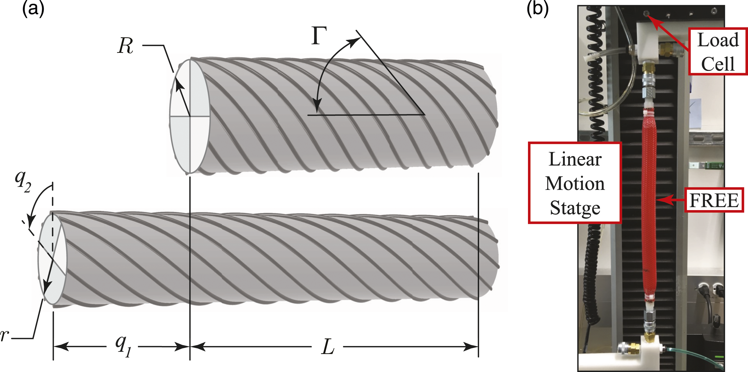q = 0 and (bottom) a deformed configuration. To verify the theoretical predictions, we tested a special type of FREE, a McKibben muscle, in a tensile testing machine (b).

The assumption that a FREE is cylindrical with inextensible fibers implies that changes in its radius, length, and twist are coupled. Therefore, its geometrical deformation can be fully defined in terms of just two parameters, a change in its length q₁ and a twist about its long axis q₂. These two variables simultaneously constitute the vector of task space motion and of generalized deformations. Consequently, the vector F describes a force along the main axis and a torsional moment about that axis. There is no internal motion.

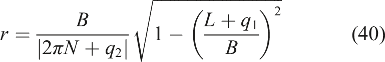
To arrive at an expression for the volume of the free, we first compute the length and radius of the deformed FREE according to:

$\begin{array}{ll}l& =L+q_1,\end{array}$

(39)

$\begin{array}{ll}r& =\frac{B}{\left|2\pi N+q_2\right|}\sqrt{1-{\left(\frac{L+q_1}{B}\right)}^2}\end{array}$

(40)

and express the volume as

$\begin{array}{ll}V\left(\mathit{q}\right)& =\pi r^{2}l\\ & =\frac{\pi \left(L+q_1\right){(B^2-\left(L+q_1\right)}^2)}{{\left(2\pi N+q_2\right)}^2}\end{array}$

(41)

With this, the Fluid Jacobian is determined to be:

${\mathit{J}}_{\mathrm{v}}\left(q\right)={\left[\begin{array}{c}\frac{\pi \left(B^2-3{\left(L+q_1\right)}^2\right)}{{\left(2\pi N+q_2\right)}^2}\\ \frac{2\pi \left(L+q_1\right)\left({\left(L+q_1\right)}^2-B^2\right)}{{\left(2\pi N+q_2\right)}^3}\end{array}\right]}^{\mathrm{T}}$

(42)

and the force generated by the FREE is given by:

$\mathit{F}={\mathit{J}}_{\mathrm{v}}^{\mathrm{T}}p+{\mathit{\tau }}_{\mathrm{E}}$

(43)

where the elastic forces τ _E could be, for example, represented by a linear force model τ _E = − Kq .

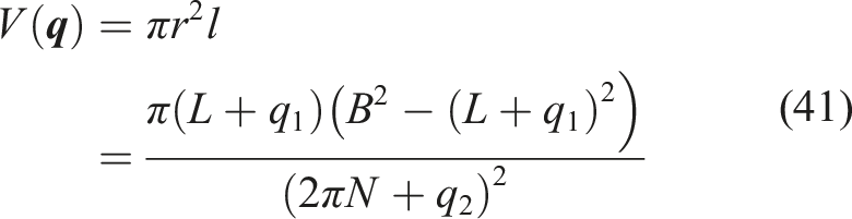
We experimentally verified these theoretical predictions through a set of measurements on a so called McKibben muscle Tondu (2012), a special type of FREE, wherein two sets of fibers are wrapped at equal and opposite angles. This prevents any twist of the actuator, leading to the special case of q₂ = F₂ = 0. The particular muscle that we tested had fibers of length B = 29.8 cm and number of revolutions N = 3.3. It consisted of a bladder made of a non-elastic material (Stretchlon 200) surrounded by a braided sheath of inextensible fibers. Rather than stretching upon pressurization, the bladder unfurled to the maximum volume allowed by the fiber constraints. Thus, elastic forces τ _E were assumed to be negligible.

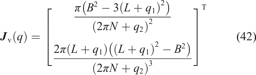
This McKibben muscle was installed in a tensile testing machine (Instron 6800 Series single column), using custom made pneumatic connectors (Figure 2(b)). The pressure inside the McKibben was fixed while the ends were slowly pulled apart. The resulting forces as a function of length were recorded for pressures of 34, 69, 103, and 138 kPa and compared to the force predictions according to (43) (Figure 3(a)). The Fluid Jacobian predictions have an RMSE over all trials of 5.1 N, with the maximum force magnitude measured being 125 N.

Figure 3.

Shown in (a) are the theoretical prediction (solid line, based on equation (43)) and experimental measurements (circles) of the force generated by a McKibben actuator as a function of actuator length l. For (b), we plotted the force divided by the pressure and compare it against the theoretical prediction of the value of the Fluid Jacobian (based on equation (42)). Note that the Fluid Jacobian is negative, as the actuator creates a pulling force.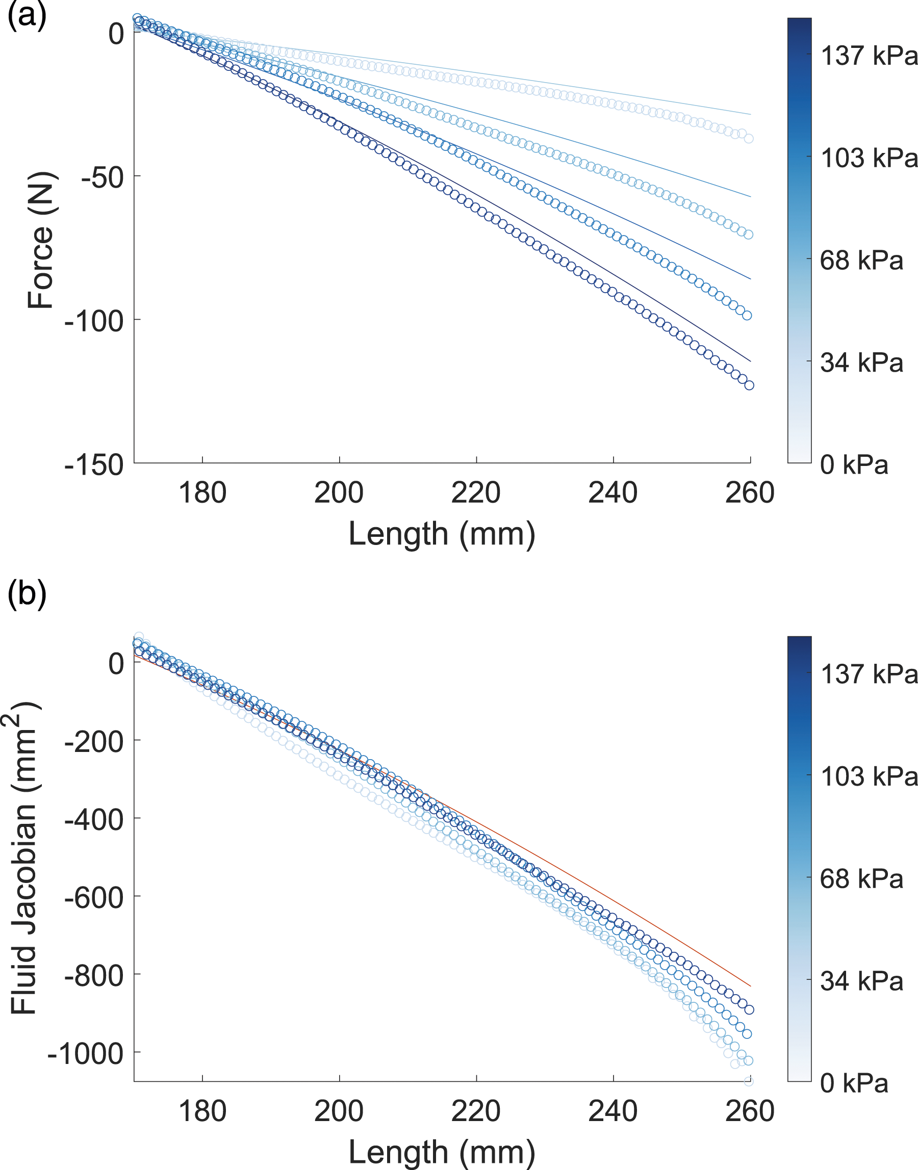

As the length increases, so does the error of the Jacobian predictions. This deviation may be due to a source of unmodeled elasticity, which we would expect to contribute larger forces as the length increases. Yet, even without explicitly accounting for this elasticity, the agreement between the Fluid Jacobian and measured data is on par with existing models. When comparing theoretically predicted and measured forces, the Fluid Jacobian produced RMS errors of around 4% of the full range, which is comparable to the best results from Sedal et al. (2021), which achieved an average normalized error of 5.5% using a learned neural network model. While the data in Sedal et al. (2021) was recorded on a FREE with elastic elements, it also required the fitting of 62 model parameters. In general, for static force models of McKibben muscles, “an experimental estimate higher in accuracy than about 5% is difficult to obtain” Tondu (2012).

Figure 3(b) shows the theoretical Fluid Jacobian compared to the actual force divided by pressure at every point. The experimental data matches the theoretical Jacobian with a RMSE of 75.7 mm², and the maximum measured value of the force divided by pressure was 844 mm². In both theory and measurement, we observe a singular configuration of the FREE at a length of 172 mm and a fiber angle of 54.7°. In this configuration, the Fluid Jacobian is equal to zero, which corresponds to a local maximum in the FREE volume. Since the muscle seeks to maximize its volume, the actuator “locks” and does not produce any force. In the literature, this singular configuration is known as the “magic angle” Demirkoparan and Pence (2015). At lengths below this threshold, the muscle generates positive (pushing) forces.

A more detailed description of modeling this class of actuators with the Fluid Jacobian can be found in Bruder et al. (2018b). Here, the approach is also exploited to predict the force generation of parallel combinations of FREEs. A comparison of the predictive capabilities of different modeling approaches, including the one based on the Fluid Jacobian and linear elastic forces can be found in Sedal et al. (2021).

3.3 Six-plate actuator

In this example, we consider an origami-style actuator consisting of six hinged plates (Figure 4(a)). For the theoretical derivation of the Fluid Jacobian, we treated the system as a quasi-planar structure with depth d. The top and bottom plates both have a length of l₁, and the connecting plates a length of l₂. The top plate is guided, such that it can only move vertically without rotation. This vertical translation, which also constitutes the task space of the system, is described by the configuration variable h, the height of the actuator. The actuator thus has a prismatic action, similar to that of a hydraulic or pneumatic cylinder. However, the transmission ratio between the force F and a given internal pressure p (as it is provided by the Fluid Jacobian) is state-dependent.

Figure 4.

In this example, we consider an origami-type actuator made from six rigid hinged plates. The top plate of the actuator is constrained, such that it can only move vertically. The actuator is shown as a schematic in (a), while the actual experimental test rig is shown in (b). In the experiments, actuator height h, Volume V, pressure p, and forces F were varied and measured.

To highlight the use of the constrained formulation in equations (24) and (25), we use non-minimal coordinates to describe this system. In particular, we include the folding angle θ of the connecting plates as an auxiliary variable, such that the complete configuration is given as $\mathit{q}={\left[\begin{array}{ll}h& \theta \end{array}\right]}^T$ . Notably, the system has a kinematic singularity at θ = π/2, and in the following, we limit ourselves to “ $>\hspace{0.17em}<$ ”-configurations, in which the side walls fold inward (θ ≤ π/2). The forward kinematics function is given as $\mathit{f}\left(\mathit{q}\right)=h$ , there is no elastic energy storage $\left(e\left(\mathit{q}\right)=0\right)$ , and the additional constraints are $\mathit{g}\left(\mathit{q}\right)=h-2l_2\sin \hspace{0.17em}\theta$ . The internal volume is given as:

$\mathit{v}\left(\mathit{q}\right)=d{l}_{1}h-d{l}_{2}h\hspace{0.17em}\cos \hspace{0.17em}\theta .$

(44)

These functions lead to:

$\begin{array}{ll}{\mathit{J}}_{\mathrm{x}}& =\left[\begin{array}{ll}1& 0\end{array}\right]\end{array}$

(45)

$\begin{array}{ll}{\mathit{J}}_{\mathrm{v}}& =\left[\begin{array}{ll}d{l}_1-d{l}_2\cos \hspace{0.17em}\theta & d{l}_{2}h\hspace{0.17em}\sin \hspace{0.17em}\theta \end{array}\right]\end{array}$

(46)

$\begin{array}{ll}{\mathit{\tau }}_{\mathrm{E}}& =0\end{array}$

(47)

$\begin{array}{ll}{\mathit{J}}_{\mathrm{g}}& =\left[\begin{array}{ll}1& -2l_{2}h\hspace{0.17em}\cos \hspace{0.17em}\theta \end{array}\right]\end{array}.$

(48)

To account for the additional constraints, we introduce $\mathit{Q}=\left[\begin{array}{ll}2l_{2}h\hspace{0.17em}\cos \hspace{0.17em}\theta & 1\end{array}\right]$ , for which it is straightforward to verify J _g Q ^T = 0. With this, we can compute: ${\mathit{J}}_{\overline{\mathrm{x}}}=2l_2\cos \hspace{0.17em}\theta$ , ${\mathit{J}}_{\overline{\mathrm{x}}}^{+}=1/\left(2l_2\cos \hspace{0.17em}\theta \right)$ , and obtain a vanishing ${\mathit{J}}_{\overline{\mathrm{y}}}$ . Consequently, the Fluid Jacobian is:

$\begin{array}{ll}{\mathit{J}}_{\mathrm{v},\mathrm{x}}& =d\left(l_1-l_2\cos \hspace{0.17em}\theta +\frac{1}{2}\tan \hspace{0.17em}\theta h\right)\\ & =d\left(l_1-\frac{\sqrt{4l_2^2-h^2}}{2}+\frac{h^2}{2\sqrt{4l_2^2-h^2}}\right),\end{array}$

(49)

with the substitution: $\theta ={\sin }^{-1}\left(h/2l_2\right)$ . From this, we get the following model for the relationship of forces and pressure:

$F=d\left(l_1-\frac{\sqrt{4l_2^2-h^2}}{2}+\frac{h^2}{2\sqrt{4l_2^2-h^2}}\right)p.$

(50)

In addition to the theoretical analysis, we also performed an experimental validation of the transmission capabilities of this system. To this end, a folding structure was made from 3D-printed plates. Metal rods were used as hinges to connect the side plates with the top/bottom plate, while the joints between the side plates were made from adhesive tape. The chosen dimensions were l₁ = 57.15 mm, l₂ = 31.12 mm, and d = 50.80 mm. To contain the fluid volume, an inflatable pouch made from an inextensible Mylar membrane was inserted into the actuator. To prevent the extension of this pouch in the direction of the open ends at the front and back of the actuator, two acrylic plates were put in place. The actuator was installed in a test rig that constrained the system to axial motion (Figure 4(b)). Two separate experiments were performed in order to determine the Fluid Jacobian of the actuator and its effect on power transmission.

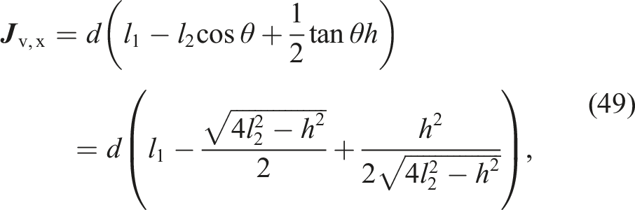
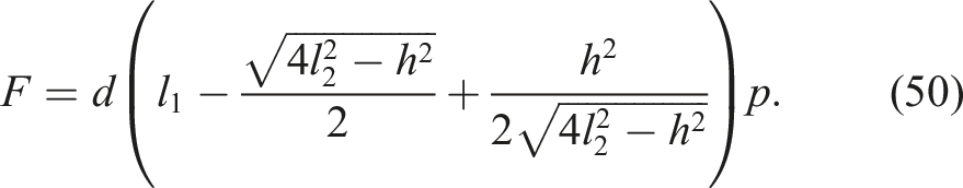
In the first experiment, we measured the change in height h (using a USDigital EM2 Optical Encoder) while inserting a known volume V of water into the actuator. Height started at 12.70 mm (with an initial volume of 7.5 mL) and water was injected in increments of 2.0 mL using a 20.0 mL medical syringe until a volume of 173.5 mL was reached, close to the actuator’s kinematic singularity. This volume data is shown in Figure 5(a) in comparison to the theoretical volume prediction from equation (44). The theoretical prediction matched the experimental measurements with an RMSE of 6.8 mL. From this data, we computed an experimental Fluid Jacobian by numerically evaluating the partial derivative $\partial V/\partial h$ via finite differences using the gradient() function in MATLAB. Data were not filtered for this step. In Figure 5(b), this experimentally obtained Fluid Jacobian is compared to the prediction of equation (49). This prediction matched the derivative of the measurements with an RMSE of 60.7 cm² (The RMSE value is dominated by the data close to the singularity. If we exclude the 6 data points with forces $>$ 100 N, the RMSE reduces to 8.7 cm²). The largest measured Fluid Jacobian value was 525 cm².

Figure 5.

Shown in (a) are the theoretical prediction, based on equation (44), and experimental measurements of the volume of the six-plate actuator as a function of actuator height (h) For (b), we took the partial derivative of these data and compare it against the theoretical prediction of the value of the Fluid Jacobian based on equation (49).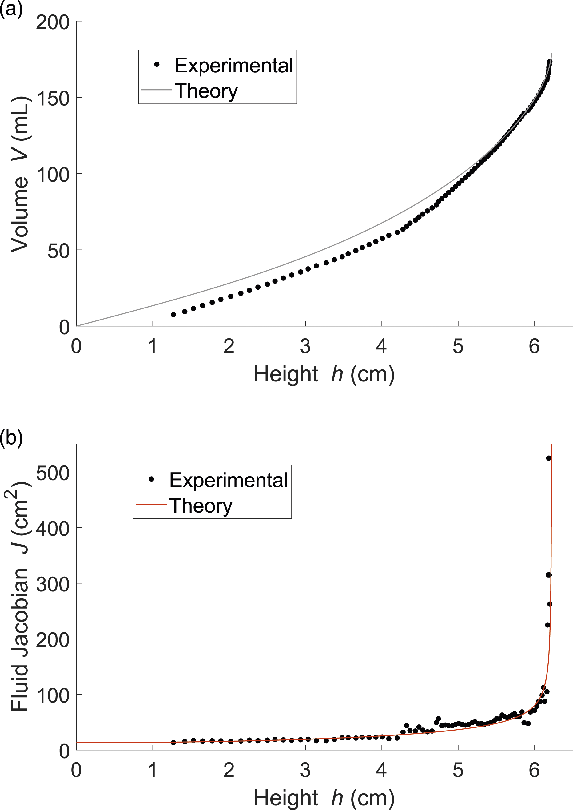

In the second experiment, we used the actuator with compressed air and measured actuator force F as a function of height h and pressure p. Force F was measured using a load cell (HT Sensor Technology Co. TAL220B) with a force measurement range of 50 N. Height h was varied in increments of 6.35 mm starting at 12.70 mm. It was adjusted manually with a lockable linear slide and measured via the linear encoder. An Enfield TR-010-g10-s electronic pressure regulator was used to apply seven different pressure values p. For these pressure values, the measured forces are shown in Figure 6(a) as a function of actuator height h and compared with the predictions from equation (50). Here, the theoretical force predictions matched the measurements with an overall RMSE of 3.0 N, compared to an overall range of forces of 47 N. From this data, we computed an equivalent Fluid Jacobian from the ratio F/p. This data is shown in Figure 6(b). The theoretical prediction of the Fluid Jacobian matched the ratio of forces and pressures with an RMSE of 8.2 cm². In this experiment, the maximum value of the Fluid Jacobian was 75 cm².

Figure 6.

Shown in (a) are the theoretical predictions of actuator forces F (solid lines, based on equation (50)) and experimental measurements for seven different values of pressure p. In addition, we computed an equivalent Fluid Jacobian value from the ratio F/p, which is compared to the theoretical prediction from equation (49) in (b).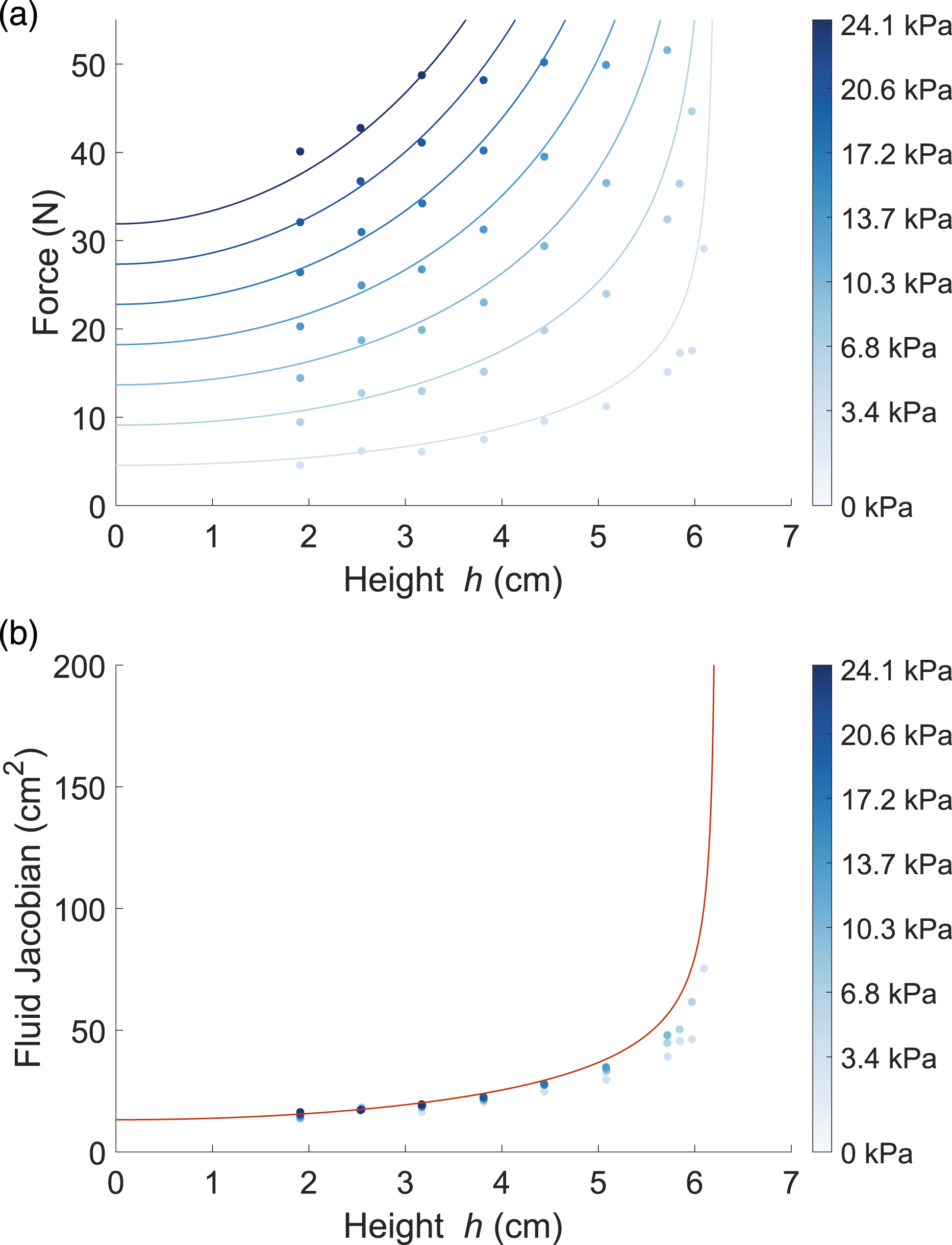

In this example, the origami-style folding structure of the presented actuator yields a Fluid Jacobian that is highly dependent on the state h. In particular, close to the kinematic singularity of the actuator (for θ = pi/2), the effective area of power transmission is almost a factor of 20 larger than the size of the top plate of the actuator. Such a state-dependent force amplification could be used, for example, as part of a continuously variable transmission which, for a given internal pressure, can greatly amplify the force output of the enclosed inflatable based on the configuration of the mechanism Brei and Gillespie (2022).

In the experimental evaluation, we saw that the simplified geometric model of the internal volume, which completely ignored the effect of the Mylar pouch, worked quite well and very closely predicted the measured volume values. In turn, the “experimental” Fluid Jacobian that was obtained by taking the partial derivative of the height–volume measurements, very closely matched the theoretical prediction, as well. This close match was achieved without any filtering or smoothing of the raw data, which was also generated in a rather crude way by means of a medical syringe. We believe that more carefully recorded data, for example, using a constant displacement pump, and appropriate filtering prior to taking partial derivatives could yield a Fluid Jacobian that is on par with one derived from the geometry of the actuator. This approach could be very useful when characterizing soft actuators with complex geometries and a high-dimensional internal motion space.

When comparing theoretically predicted and measured forces, the Fluid Jacobian produced RMS errors of around 6% of full range. Figure 6(b) also nicely illustrates the linearity of forces and pressure. In this normalized view of the ratio F/p, the data points at a given displacement overlap fairly closely.

3.4 Six-plate actuator with internal motion

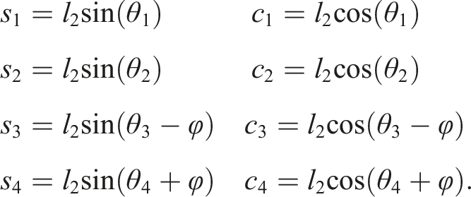
In this final example, we want to revisit the six plate actuator from Section 3.3 and remove the physical constraint that restricts the motion of the top plate to purely vertical or axial motion. That is, the top plate can now move vertically in h, laterally in r, and it can pitch with an angle of φ. We still only consider h to constitute the useful motion of the actuator, while r and φ would be part of the internal motion. To enable this additional motion, we need to account for the fact that the four angles of the connecting plates can now all be different (Figure 7). The overall configuration vector for this extended system thus is $\mathit{q}={\left[\begin{array}{lllllll}r& h& \phi & {\theta }_1& {\theta }_2& {\theta }_3& {\theta }_4\end{array}\right]}^{\mathrm{T}}$ . The forward kinematics function still is $\mathit{f}\left(\mathit{q}\right)=h$ , such that ${\mathit{J}}_{\mathrm{x}}=\left[\begin{array}{lllllll}0& 1& 0& 0& 0& 0& 0\end{array}\right]$ . We can compute the volume, just using the angles θ _i as:

$\begin{array}{ll}V& =\frac{d{l}_1{l}_2}{2}\left(\sin {\theta }_1+\sin {\theta }_2+\sin {\theta }_3+\sin {\theta }_4\right)\hspace{1em}\dots \\ & -\frac{d{l}_2^2}{2}\left(\sin \left({\theta }_1+{\theta }_2\right)+\sin \left({\theta }_3+{\theta }_4\right)\right)\end{array}$

(51)

with the volume Jacobian:

${\mathit{J}}_{\mathrm{v}}={\left[\begin{array}{c}0\\ 0\\ 0\\ \frac{d{l}_1{l}_2}{2}\cos {\theta }_1-\frac{d{l}_2^2}{2}\cos \left({\theta }_1+{\theta }_2\right)\\ \frac{d{l}_1{l}_2}{2}\cos {\theta }_2-\frac{d{l}_2^2}{2}\cos \left({\theta }_1+{\theta }_2\right)\\ \frac{d{l}_1{l}_2}{2}\cos {\theta }_3-\frac{d{l}_2^2}{2}\cos \left({\theta }_3+{\theta }_4\right)\\ \frac{d{l}_1{l}_2}{2}\cos {\theta }_4-\frac{d{l}_2^2}{2}\cos \left({\theta }_3+{\theta }_4\right)\end{array}\right]}^{\mathrm{T}}.$

(52)

Figure 7.

We further examine the actuator from Section 3.3, to include lateral and pitching motion of the top plate (given by r and φ). In this 2D view of the actuator, the additional configuration variables are introduced.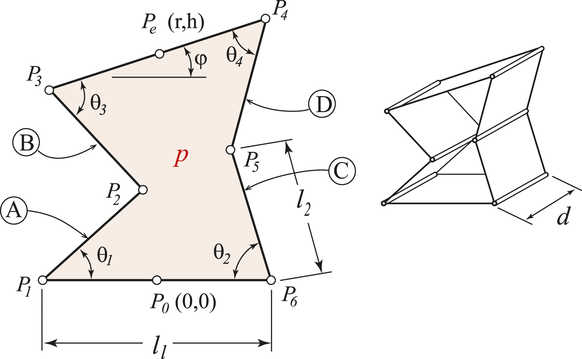

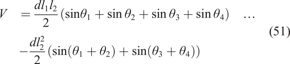
Two vector loop equations can be used to produce four scalar constraint equations (Figure 7). The first goes from P₀ over P₁, P₂, and P₃ to P _e (along the links A and B), while the second goes from P₀ over P₆, P₅, and P₄ to P _e (along the links C and D). These are transcendental equations that can be expressed in implicit form in $\mathit{g}\left(\mathit{q}\right)=\mathbf{0}$ , with:

$g=\left[\begin{array}{l}r+\frac{l_1}{2}-c_1+c_3-\frac{l_1}{2}\cos \hspace{0.17em}\phi \\ h+0-s_1-s_3-\frac{l_1}{2}\sin \hspace{0.17em}\phi \\ r-\frac{l_1}{2}+c_2-c_4+\frac{l_1}{2}\cos \hspace{0.17em}\phi \\ h-0-s_2-s_4+\frac{l_1}{2}\sin \hspace{0.17em}\phi \end{array}\right]$

(53)

with

$\begin{array}{llll}{s}_1& =l_2\sin \left({\theta }_1\right)& c_1& =l_2\cos \left({\theta }_1\right)\\ s_2& =l_2\sin \left({\theta }_2\right)& c_2& =l_2\cos \left({\theta }_2\right)\\ s_3& =l_2\sin \left({\theta }_3-\phi \right)& c_3& =l_2\cos \left({\theta }_3-\phi \right)\\ s_4& =l_2\sin \left({\theta }_4+\phi \right)& c_4& =l_2\cos \left({\theta }_4+\phi \right).\end{array}$

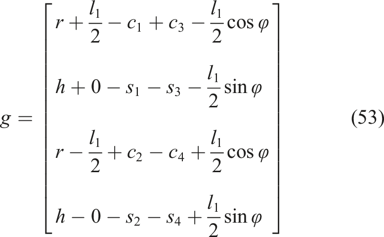
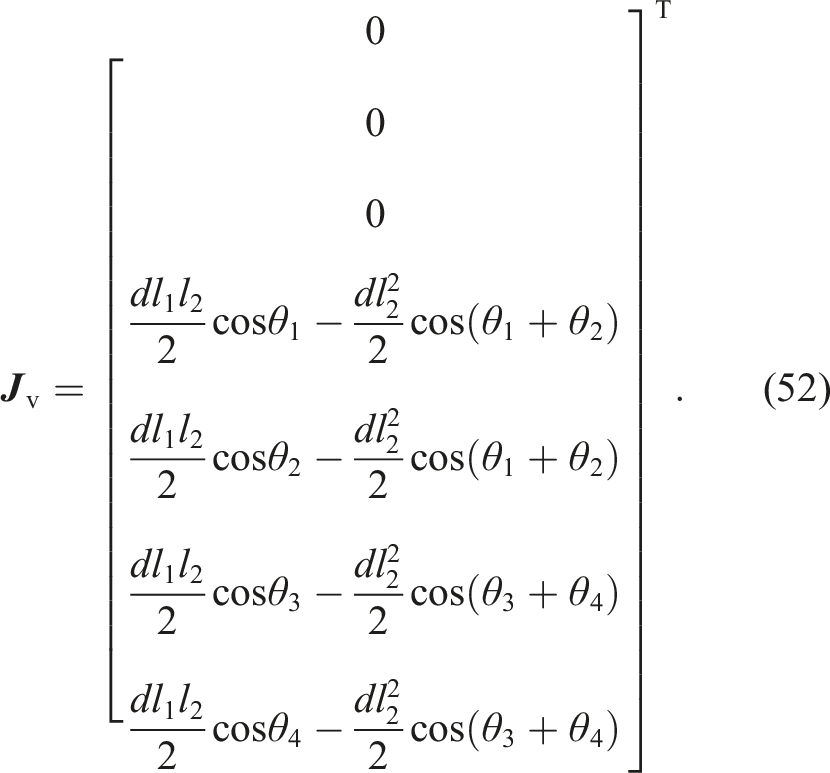
Differentiation with respect to q yields the constraint Jacobian:

${\mathit{J}}_{\mathrm{g}}=\left[\begin{array}{lllllll}1& 0& \frac{l_1}{2}\sin \hspace{0.17em}\phi +s_3& s_1& 0& -s_3& 0\\ 0& 1& -\frac{l_1}{2}\cos \hspace{0.17em}\phi +c_3& -c_1& 0& -c_3& 0\\ 1& 0& -\frac{l_1}{2}\sin \hspace{0.17em}\phi +s_4& 0& -s_2& 0& s_4\\ 0& 1& \frac{l_1}{2}\cos \hspace{0.17em}\phi -c_4& 0& -c_2& 0& -c_4.\end{array}\right]$

(54)

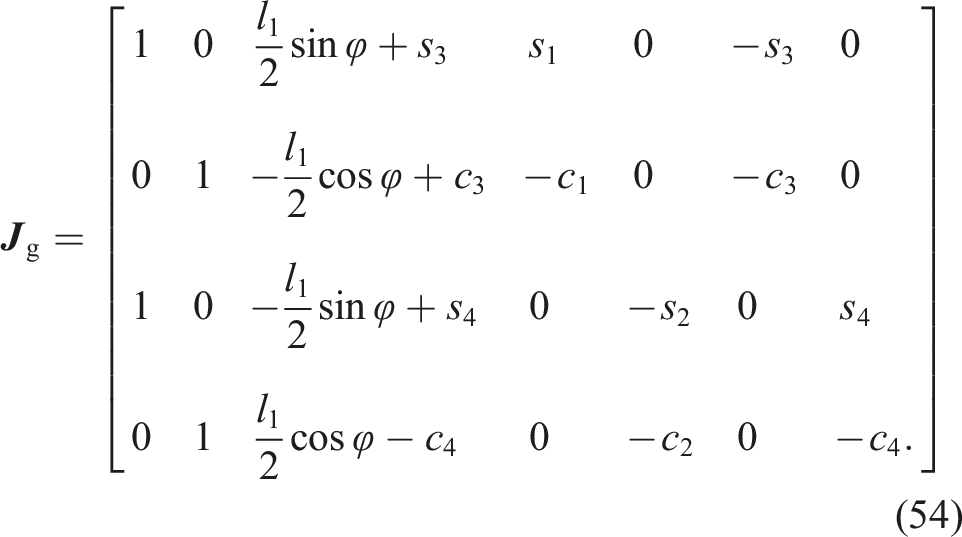
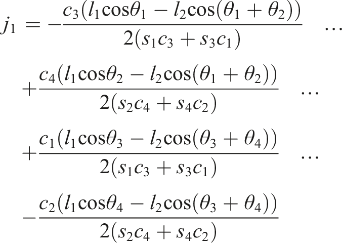
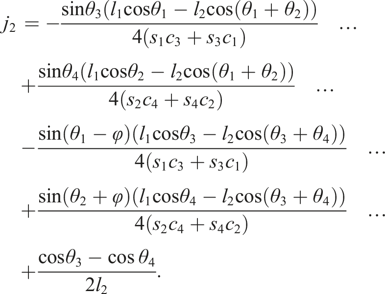
The following is an orthogonal complement to this matrix J _g, with J _g Q = 0:

$\mathit{Q}=\left[\begin{array}{ccc}1& 0& 0\\ 0& 1& 0\\ 0& 0& 1\\ \frac{-c_3}{s_1{c}_3+s_3{c}_1}& \frac{s_3}{s_1{c}_3+s_3{c}_1}& \frac{-l_1{l}_2\sin {\theta }_3}{2\left(s_1{c}_3+s_3{c}_1\right)}\\ \frac{c_4}{s_2{c}_4+s_4{c}_2}& \frac{s_4}{s_2{c}_4+s_4{c}_2}& \frac{l_1{l}_2\sin {\theta }_4}{2\left(s_2{c}_4+s_4{c}_2\right)}\\ \frac{c_1}{s_1{c}_3+s_3{c}_1}& \frac{s_1}{s_1{c}_3+s_3{c}_1}& \frac{-l_1{l}_2\sin \left({\theta }_1-\phi \right)}{2\left(s_1{c}_3+s_3{c}_1\right)}+1\\ \frac{-c_2}{s_2{c}_4+s_4{c}_2}& \frac{s_2}{s_2{c}_4+s_4{c}_2}& \frac{l_1{l}_2\sin \left({\theta }_2+\phi \right)}{2\left(s_2{c}_4+s_4{c}_2\right)}-1\end{array}\right]$

(55)

with this choice of Q , the minimal coordinates are equal to the three degrees of freedom of the top plate $\left({\mathit{q}}_{\min }={\left[\begin{array}{lll}r& h& \phi \end{array}\right]}^T\right)$ . These three coordinates, in a sense, become the independent coordinates, while the θ _i become the dependent coordinates. Out of this choice of minimal coordinates, h would constitute the task space motion, while r and φ describe the internal motion. This is reflected in the Jacobians:

$\begin{array}{llll}{\mathit{J}}_{\overline{\mathrm{x}}}& =\left[\begin{array}{lll}0& 1& 0\end{array}\right]& {\mathit{J}}_{\overline{\mathrm{y}}}& =\left[\begin{array}{lll}1& 0& 0\\ 0& 0& 1\end{array}\right]\end{array}$

(56)

$\begin{array}{llll}{\mathit{J}}_{\overline{\mathrm{x}}}^{+}& =\left[\begin{array}{l}0\\ 1\\ 0\end{array}\right]& {\mathit{J}}_{\overline{\mathrm{y}}}^{+}& =\left[\begin{array}{ll}1& 0\\ 0& 0\\ 0& 1\end{array}\right]\end{array}.$

(57)

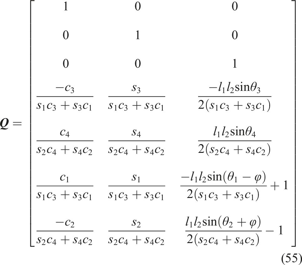
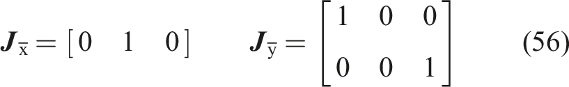
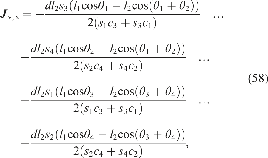
We now can go ahead and compute the Task Space Fluid Jacobian:

$\begin{array}{ll}{\mathit{J}}_{\mathrm{v},\mathrm{x}}& =+\frac{d{l}_2{s}_3\left(l_1\cos {\theta }_1-l_2\cos \left({\theta }_1+{\theta }_2\right)\right)}{2\left(s_1{c}_3+s_3{c}_1\right)}\hspace{1em}\dots \\ & +\frac{d{l}_2{s}_4\left(l_1\cos {\theta }_2-l_2\cos \left({\theta }_1+{\theta }_2\right)\right)}{2\left(s_2{c}_4+s_4{c}_2\right)}\hspace{1em}\dots \\ & +\frac{d{l}_2{s}_1\left(l_1\cos {\theta }_3-l_2\cos \left({\theta }_3+{\theta }_4\right)\right)}{2\left(s_1{c}_3+s_3{c}_1\right)}\hspace{1em}\dots \\ & +\frac{d{l}_2{s}_2\left(l_1\cos {\theta }_4-l_2\cos \left({\theta }_3+{\theta }_4\right)\right)}{2\left(s_2{c}_4+s_4{c}_2\right)},\end{array}$

(58)

and the Internal Motion Fluid Jacobian:

${\mathit{J}}_{\mathrm{v},\mathrm{y}}=\left[\begin{array}{ll}{j}_{1}d{l}_2& j_{2}d{l}_1{l}_2^2\end{array}\right],$

(59)

with

$\begin{array}{ll}{j}_1& =-\frac{c_3\left(l_1\cos {\theta }_1-l_2\cos \left({\theta }_1+{\theta }_2\right)\right)}{2\left(s_1{c}_3+s_3{c}_1\right)}\hspace{1em}\dots \\ & +\frac{c_4\left(l_1\cos {\theta }_2-l_2\cos \left({\theta }_1+{\theta }_2\right)\right)}{2\left(s_2{c}_4+s_4{c}_2\right)}\hspace{1em}\dots \\ & +\frac{c_1\left(l_1\cos {\theta }_3-l_2\cos \left({\theta }_3+{\theta }_4\right)\right)}{2\left(s_1{c}_3+s_3{c}_1\right)}\hspace{1em}\dots \\ & -\frac{c_2\left(l_1\cos {\theta }_4-l_2\cos \left({\theta }_3+{\theta }_4\right)\right)}{2\left(s_2{c}_4+s_4{c}_2\right)}\end{array}$

and

$\begin{array}{ll}{j}_2& =-\frac{\sin {\theta }_3\left(l_1\cos {\theta }_1-l_2\cos \left({\theta }_1+{\theta }_2\right)\right)}{4\left(s_1{c}_3+s_3{c}_1\right)}\hspace{1em}\dots \\ & +\frac{\sin {\theta }_4\left(l_1\cos {\theta }_2-l_2\cos \left({\theta }_1+{\theta }_2\right)\right)}{4\left(s_2{c}_4+s_4{c}_2\right)}\hspace{1em}\dots \\ & -\frac{\sin \left({\theta }_1-\phi \right)\left(l_1\cos {\theta }_3-l_2\cos \left({\theta }_3+{\theta }_4\right)\right)}{4\left(s_1{c}_3+s_3{c}_1\right)}\hspace{1em}\dots \\ & +\frac{\sin \left({\theta }_2+\phi \right)\left(l_1\cos {\theta }_4-l_2\cos \left({\theta }_3+{\theta }_4\right)\right)}{4\left(s_2{c}_4+s_4{c}_2\right)}\hspace{1em}\dots \\ & +\frac{\cos {\theta }_3-\cos {\theta }_4}{2l_2}.\end{array}$

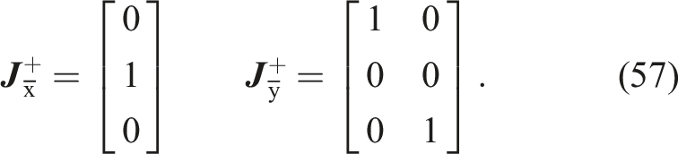
For the case of a vertical and centered top plate, that is, for φ = r = 0, the four internal angles need to be equal: θ₁ = θ₂ = θ₃ = θ₄ = θ. In this case, the Task Space Fluid Jacobian becomes:

${\mathit{J}}_{\mathrm{v},\mathrm{x}}=d{l}_1-d{l}_2\frac{\cos \left(2\theta \right)}{\cos \hspace{0.17em}\theta }$

(60)

which is identical to equation (49) for h = 2L₂ sin θ. More importantly, for this choice of configuration variables, the Internal Motion Fluid Jacobian vanishes:

${\mathit{J}}_{\mathrm{v},\mathrm{y}}=\left[\begin{array}{ll}0& 0\end{array}\right].$

(61)

Equation (61) is a case of a fluid singularity, in which the Fluid Jacobian vanishes. More specifically, the internal volume of the actuator becomes maximal for φ = r = 0. That is, as long as no elastic forces are being applied, any positive pressure will move the internal degrees of freedom φ and r into this configuration, as shown in equation (11). The additional mechanical constraints that were introduced in the experimental setup of Section 3.3 to limit the motion of the top plate to be purely vertical, are thus superfluous and could potentially be avoided while still creating a purely vertical force.

4. Discussion

In this paper, we introduced the concept of the Fluid Jacobian, which provides a framework to model the relationship between task space forces and fluid pressure in fluid-driven soft robotic systems. In a sense, the Fluid Jacobian can be regarded as a generalization of the cross-sectional area of a piston in a traditional hydraulic or pneumatic cylinder. In fact, in the introductory example of the double cylinder in Section 3.1, the Fluid Jacobians are exactly identical to the cross sections of the two cylinders (equations (29) and (30)).

The first key difference, compared to hydraulic/pneumatic cylinders, is that Fluid Jacobians can be multi-dimensional and couple multiple actuators to a multi-dimensional task space motion. In a well-defined actuator system, the Task Space Fluid Jacobian should be square and invertible, such that a given number of degrees of freedom in the task space is driven by an equal number of actuators. If this is not the case for a certain actuator type, one can either introduce additional kinematic constraints on the task space (as done in the experiments in Sedal et al. (2021)) or combine multiple actuators to work in parallel (as done in Bruder et al. (2018b)). Otherwise, the uncontrollable dimensions should be removed from the task space and regarded as part of the internal motion space.

As a second key difference, and in stark contrast to the cross sections in hydraulic/pneumatic cylinders, Fluid Jacobians are configuration dependent; that is, they are functions of q . This can be seen, for example, in the case of the FREE in Section 3.2 (equation (42)) and the six-plate actuator in Section 3.3 (equation (49)). This configuration-dependency gives rise to the possibility of additional singularities in the robotic system. We refer to them as fluid singularities. In contrast to kinematic singularities (that we explicitly excluded in the assumptions of Section 2.1), the robotic system is not subject to a reduction in its DOFs. Instead, the volumes of individual actuator cells become linearly coupled with respect to the configuration. As a consequence, and according to the loss of rank in the Jacobian, the dimensions of the achievable task-force directions are reduced. A special case is one in which singularities cause an entire row of the Fluid Jacobian to become zero. For single actuators, this is the only possible fluid singularity. In this case, the internal volume of the corresponding actuator becomes maximal (minimal) and cannot expand (contract) further in the presence of positive (negative) pressure. The actuator cell “locks.” For the FREE actuator, for example, this effect is known as the “magic angle” Demirkoparan and Pence (2015); Krishnan et al. (2015), and occurs at a fiber angle of 54.7°. We believe that such fluid singularities and the associated locking effects will provide ample space for further research on the design and control of soft robotic systems. For example, and as discussed above, fluid singularities are an important effect to limit unwanted internal motion.

By introducing the Fluid Jacobian, our work helps establish structure in the fundamental relationship of forces F , pressures p , and configurations q in fluid-driven soft actuator systems. The most general case for this structure was given by the force balances in equations (7) and (8) which provide conditions for the static equilibria in the task space and internal motion space, respectively. Notably, pressure enters both equations linearly by means of the Fluid Jacobians J _v,x and J _v,y. Without degrees of freedom of internal motion y , or without elastic energy storage in the actuator system τ _E, this linearity is preserved at the output, and task space forces are proportional to the applied pressures via the Fluid Jacobian J _v,x (equations (9) and (12)). For these special cases, the Fluid Jacobians only depend on the task space configuration x . As soon as the actuator system allows for an internal motion against an elastically deformable structure, this linearity is lost. In this case, varying pressures p change the internal configuration y , which in turn influences the Fluid Jacobians and the elastic forces in the task space. This results in a nonlinear relationship between forces F and pressures p as described by equation (14).

Beyond establishing structure to equation (1), the Fluid Jacobian also has practical relevance, as demonstrated by the examples in this paper and in previous work. Since it highlights a fundamentally linear relationship between forces and pressures, the concept is particularly well suited for control applications, and can be easily extended to describe systems of multiple actuators. This has been shown, for example, in Bruder et al. (2018b), where the Fluid Jacobian was used to estimate the workspace of different soft manipulator designs.

The predictive capabilities of models based on the Fluid Jacobian are on par with other modeling approaches, as demonstrated by the experimental evaluation of the FREE and the six-plate actuator in Sections 3.2 and 3.3. A more detailed analysis of this modeling approach and a comparison with learned models and predictions based on continuum mechanic models can be found in Sedal et al. (2021). Sedal et al. show that a prediction based on the fluid Jacobian with a linear stiffness model (for which the coefficients were fitted to the evaluated actuator) has an average error of 17.4% compared to 17.0% for a continuum model and 5.51% for a neural network. These numbers change when the parameters are identified based on a different actuator than the one evaluated. In this case, the fluid Jacobian model has a mean error of 29.3%, the continuum model of 17.3%, and the neural network of 30.4%. That is, while not being the most accurate model in absolute terms, the predictions of the Fluid Jacobian extrapolate better than a learned model and have the benefit of computational simplicity compared to finite element models or other types of continuum mechanics models.

Soft actuators have almost inevitably some amount of internal motion y . Describing this motion and its effect on volume can be difficult, as the motion can be geometrically complex and high-dimensional. This may seem to limit the value of an analytical Fluid Jacobian for some applications. However, in many cases, the simplifying assumption of no internal motion, as discussed in Section 2.3.1, is often closely approximated in actual soft robotic systems, and equation (9) can be used to describe the force-motion relationship. In this case, the volume of the actuator system only needs to be described in terms of the task space motion x , which is much lower dimensional than the internal motion.

The reason why this approximation works well is because in many soft robotic systems, elastic internal motion is actually undesired and often minimized by design. Not following this principle is probably the biggest anomaly in the contrived example of the double cylinder in Section 3.1. In an actual hydraulic cylinder, one would clearly fix the bottom of the cylinder and one would not attach springs to the output. In other words, c₁ and c_c, would be made as soft as possible to minimize the resistance to desired motion and c₂ would be made as stiff as possible to minimize the amount of undesired internal motion. Analogous considerations apply to general soft fluidic actuators. In a sense, the primary purpose of fibers, plates, and other reinforcing components that are embedded in soft robotic systems is specifically to direct the effort into the task space and reduce internal deformation Galloway et al. (2013); Marchese et al. (2015); Rus and Tolley (2015). In FREEs, for example, a single fiber would be theoretically sufficient to create a desired behavior, yet a mesh of fibers is used in practice to restrict bulging of the elastomer, which would constitute an undesired internal motion.

It should be noted that both high stiffness of the internal motion (in the example of Section 3.1: large c₂) and a low stiffness combined with an extremal volume (as shown in the example in Section 3.4) each lead to a Task Space Fluid Jacobian that is independent of pressure. These features in turn lead to a linear force/pressure relationship. In the first case, the high stiffness reduces internal motion, in the second case, the force balance in equation (8) can only be fulfilled when the Internal Motion Fluid Jacobian becomes zero. This corresponds to an extremum in the volume. In other words, the internal motion will seek to maximize (for positive pressure) or minimize (for vacuum) the volume of the actuator. As long as the pressure is nonzero, the internal motion is independent of the actual pressure value. These effects are also visible in the linearized model in equation (21).

In many cases, deriving Fluid Jacobians from an analytical expression of the actuators’ volume can provide the most rapid way of arriving at a force-pressure relationship. This holds in particular if fibers or other reinforcing elements make other approaches, such as determining an equivalent area manually or computing individual constraint forces, impractical. As an additional alternative, the Fluid Jacobian could be determined experimentally. In many applications of soft fluidic actuators, the internal motion has a high (if not infinite) number of dimensions and is inherently difficult to describe. In contrast, the task space is often low-dimensional, straightforward to describe, and motion in the task space is often measured with encoders or other sensors as part of a robot’s design. In such cases, the Fluid Jacobians in equations (12) and (14) could be determined experimentally. To this end, the volumes of the actuator units V must be measured over a range of task space motions and, in the case of equation (14), pressure values. The Fluid Jacobian could then be determined from these experimental values by taking the partial derivative ${\mathit{J}}_{\mathrm{v},\mathrm{x}}=\partial \mathit{V}\left(\mathit{x}\right)/\partial \mathit{x}$ or ${\mathit{J}}_{\mathrm{v},\mathrm{x}}=\partial \mathit{V}\left(\mathit{x},\mathit{p}\right)/\partial \mathit{x}$ , respectively. As demonstrated in the example of Section 3.3, such an experimentally determined Jacobian can closely match the expected values, even when using finite differences without any additional filtering or smoothing. The advantage of this method would be that it does not require the measurement of task space forces, which are not as readily accessible as task space motions.

There still is substantial potential to further extend the concept of the Fluid Jacobian. First of all, one could use it to reason about the dual relationship to force versus pressure, namely, task space velocities versus change of fluid volumes. For incompressible fluids, this relationship directly follows from the definition of the Fluid Jacobians as partial derivatives of volume against internal and task space motion, respectively. For compressible fluids, such a relationship would be more complex, as one now needs to distinguish between actuator volume, fluid mass, and fluid volume, as discussed in Stölzle and Santina (2022). In compressible fluids, fluid mass and fluid volume are related via the applied pressure. In a sense, such a compressible fluid will create a “series elastic” effect in the actuator system, similar to the effect that results from the elastic deformation due to the internal motion. ⁵

A second extension of the concept would pertain to non-traditional task spaces, which cannot be described by a small number of distinct motions. An example of such a system would be the closure of a soft gripper around a number of different objects. Instead of defining the task space of such a system via the high-dimensional geometrical deformation of the continuously compliant interaction surface, one could seek to define the task space via a number of “shape functions” that encode different gripping modes. A Fluid Jacobian could then be determined based on a limited number of such shape functions.

In summary, this paper has presented a theoretical basis and formulation of the Fluid Jacobian and given specific examples of its use and physical interpretation. By providing structure based on general power conversion laws, we hope that the Fluid Jacobian helps expand the understanding and interpretation of power transmission in fluid-mechanical systems as well as facilitates modeling, design, and control. In deriving the Fluid Jacobian, the vantage point of our work is that of a traditional roboticist. We established motion spaces and emphasized the role of the forces generated in a soft robotic system, rather than focusing on their shape and deformation. While such a force-based point of view is well established in traditional robotics, in many applications of soft robotic systems, the focus is less on the ability to generate task space forces but rather on the influence of pressure on the shape of the robot and resulting motion. This will no doubt change in the future as appropriate models for the interactions of soft robotic systems with their environments become increasingly important. Although the ultimate utility of the Fluid Jacobian in creating these models is still to be determined, in our work the Fluid Jacobian has had the distinct advantage that it enabled us to take established techniques from classical robotics, in particular kinematic Jacobians, and bring them into the world of soft robotics. Our hope is that our work has not only established a strong foundation for the use of the Fluid Jacobian but also that it will inspire the exploration of similar links between concepts well understood in traditional robotics and those important to soft robotics, such as in controller development and motion planning.