Exceeding traditional curvature limits of concentric tube robots through redundancy resolution

Abstract

Understanding elastic instability has been a recent focus of concentric tube robot research. Modeling advances have enabled prediction of when instabilities will occur and produced metrics for the stability of the robot during use. In this paper, we show how these metrics can be used to resolve redundancy to avoid elastic instability, opening the door for the practical use of higher curvature designs than have previously been possible. We demonstrate the effectiveness of the approach using a three-tube robot that is stabilized by redundancy resolution when following trajectories that would otherwise result in elastic instabilities. We also show that it is stabilized when teleoperated in ways that otherwise produce elastic instabilities. Lastly, we show that the redundancy resolution framework presented here can be applied to other control objectives useful for surgical robots, such as maximizing or minimizing compliance in desired directions.

1. Introduction

Concentric tube robots have garnered considerable interest in the continuum and surgical robotics communities in recent years. They can achieve bending and elongation via the elastic interactions of their nested, precurved tubes (see Figure 1), effects which are described by mechanics-based models (Rucker et al. 2010; Dupont et al. 2010). These devices have been applied to a number of minimally invasive surgical applications because of their small diameter and dexterity. For a review of concentric tube robotics research and applications, see (Gilbert et al. 2016a).

Figure 1.

Three-tube concentric tube robot. Each nested tube can independently translate and rotate. Concentric tube robots with highly curved tubes can “snap” from one configuration to another due to rapidly released torsional energy. Real-time control schemes must be developed that prevent these elastic instabilities from occurring during teleoperation.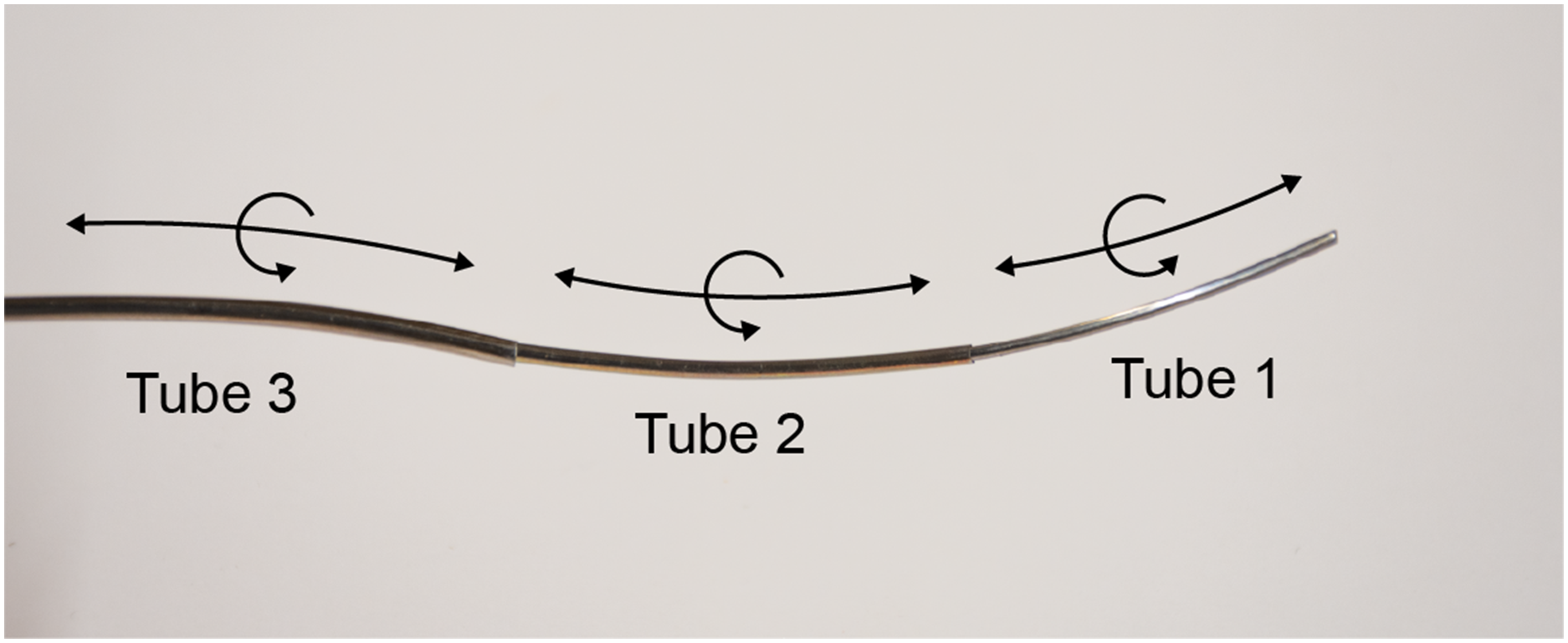

Despite many recent advancements in design, modeling, control, and practical applications, concentric tube robots have thus far been limited to maximum curvatures far below the theoretical upper limit provided by Nitinol’s maximum recoverable strain. Yet, higher curvatures are often desirable because they enable the robot to work in smaller, more constrained spaces. The reason concentric tube robots have been limited to curvatures far below the maximum recoverable strain limit of the material is that highly curved tubes, when nested within one another and axially rotated, store torsional elastic energy. If the tubes rotate too far, they will exhibit an elastic instability, rapidly releasing this energy and “snapping” from one configuration to another. This snapping effect has recently been studied from design (Hendrick et al. 2015; Bergeles et al. 2015; Luo et al. 2018; Ha et al. 2014) and modeling (Gilbert et al. 2016b; Ha et al. 2016) perspectives. Actuator motions likely to create snapping can now be predicted, and metrics for stability have been derived.

To date, elastic stability-aware control has primarily been achieved in an a priori, motion planning sense. An early metric for stability was torsional windup (Bergeles and Dupont 2013), which has been used in planning stable paths (Bergeles et al. 2015). Gilbert et al. devised a relative elastic stability metric and used it to produce stability maps for planning purposes (Gilbert et al. 2016a). These examples of stability-aware planners do not run rapidly enough to avoid snapping during real-time teleoperation. The goal of this work is to integrate instability avoidance into a real-time controller so that a user can control the robot safely.

Real-time control of concentric tube robots has been an important research topic in recent years. Several methods involve precomputation of the robot’s forward kinematics or path plans; the inverse kinematics can then be solved online at each time step using root-finding methods (Dupont et al. 2010) or a local inverse kinematics solver such as damped least squares (Torres et al. 2015). Local Jacobian-based methods seek to solve the inverse kinematics online with no need for precomputation. For example, Burgner et al. proposed a weighted damped least squares (WDLS) approach that incorporates tracking, damping, and joint limit goals (Burgner et al. 2014). This is an efficient Jacobian-based approach that can be solved at each time step with low computational burden. Other examples of Jacobian-based damped least squares control of concentric tube robots include (Fagogenis et al. 2016; Xu et al. 2013). Our proposed approach in this work uses a similar WDLS approach to (Burgner et al. 2014) that also incorporates instability avoidance and stiffness goals.

These online inverse kinematics methods have also been used for instability avoidance. Leibrandt et al. have explored rapid, online motion planning for concentric tube robots while integrating elastic stability into the framework (Leibrandt et al. 2015, 2017a). While it has been shown that it is possible to compute these replanning approaches rapidly enough for use in real time control via parallelized computing, they are computationally intensive and often require some a priori knowledge of the environment and/or the desired path. Implementation of these approaches typically requires multi-core parallel computing or graphical processing unit (GPU) computing methods. In contrast, the redundancy resolution approach we present in this paper is computationally inexpensive and requires no a priori information. Of course, the tradeoff for these advantages is that a redundancy resolution approach like ours makes no claims of global optimization to a desired final path—it will only locally optimize among competing objectives at each time step—but it is useful for teleoperation when anatomical constraints are not accurately known and/or the user’s intended path is not known a priori. The ability of our method to move the robot away from unstable configurations is also an advantage over the rapid planning method in (Leibrandt et al. 2017a); if the user enforces a particular trajectory, it is possible that the online inverse kinematics solver cannot escape local minimum due to the formulation of the stability constraint. Leibrandt et al. also used the online inverse kinematics solver to integrate dexterity goals; the dexterity measure penalizes columns of the Jacobian based on joint limits, anatomical collisions, and configuration stability (Leibrandt et al. 2017b). Since we employ a computationally efficient Jacobian-based approach, the controller moves the robot away from instability using knowledge of each joint’s effect on the robot’s stability. This is a noted limitation of (Leibrandt et al. 2017b) that arises from the high computational cost of the rapid planning GPU approach. Additional extensions in this paper beyond the work of (Leibrandt et al. 2017b, 2017a) include the integration of stiffness objectives, and experimental evaluation on a physical robot prototype. A final distinction is our use of a stability metric derived from first principles (Gilbert et al. 2016a), whereas Leibrandt et al. used a torsional windup stability metric (Bergeles and Dupont 2013).

Khadem et al. employed a redundancy resolution approach to integrating instability avoidance into an online concentric tube robot controller (Khadem et al. 2019). They used a gradient projection method in which the secondary control goal is to reshape a force-velocity manipulability ellipsoid toward a sphere to ensure that the Jacobian is full rank. Our method uses a stability metric that is derived from first principles which enables the controller to enforce an exact stability threshold. In addition, our use of a WDLS redundancy resolution formulation enables the controller to override user trajectories that will make the robot unstable, whereas null-space methods must always satisfy the primary tracking task even when that task could cause instability. An additional advantage of our approach is that it pushes the system away from instability, whereas approaches that seek to iteratively maximize manipulability, like that of Khadem et al., can sometimes push the system toward instability.

It is also desirable to control the stiffness of a concentric tube robot in real time, based on application requirements. Recognizing this, Mahvash and Dupont proposed the first stiffness controller for concentric tube robots (Mahvash and Dupont 2011). They used a deflection model to control the robot tip stiffness, based on real-time measurements of the tip location made with a magnetic tracking coil. In some applications, it may be advantageous to keep an open lumen in the concentric tube robot for surgical instruments or suction/injection, rather than consuming it with such a tracking coil, and image-based tip position sensing may be unavailable or insufficiently accurate. Yet control of tip mechanical impedance may still be useful, such as to enable the robot to gently interact with delicate tissues or forcefully interact with tissue (as must occur when a needle is being driven through tissue), as has been shown in the past with tendon-operated and multi-backbone continuum robots (e.g., see (Kim et al. 2014; Bajo and Simaan 2016)). One method for controlling tip stiffness is to examine its unified force-velocity manipulability ellipsoid (Khadem et al. 2018, 2019). In these works, the controller seeks to reshape the force-velocity manipulability ellipsoid in order to increase its force application capabilities. Our approach seeks to optimize stiffness using the compliance matrix at the tip of the robot (although different metrics could easily be incorporated into the framework).

The redundancy resolution framework we present in this paper enables simultaneous stiffness tuning and instability avoidance. Redundancy resolution has previously been applied to other kinds of continuum robots to accomplish a variety of objectives. For example, controllers for hyper-redundant robots have been developed that simultaneously command both end effector pose and backbone shape (Chirikjian and Burdick 1994, 1995). Redundancy resolution has also been used to reduce actuation forces of tendon-actuated (Camarillo et al. 2008; Yip and Camarillo 2014) and variable diameter continuum robots (Abah et al. 2018), avoid buckling in multi-backbone continuum robots (Simaan 2005), improve stability in magnetically controlled continuum catheters (Edelmann et al. 2017), avoid joint limits in multi-backbone robots (Bajo et al. 2012) and robots with multiple rolling joints (Berthet-Rayne et al. 2018), and reduce visual occlusion of the endoscope field of view during surgery (Sarli and Simaan 2017).

Toward the goal of enabling higher curvatures than have traditionally been used in continuum robot prototypes (i.e., to facilitate the stable use of robots with elastic instabilities in their workspaces) while also achieving stiffness objectives, we present a new redundancy resolution technique in this paper. Our approach makes several contributions with respect to existing literature. Compared to rapid planning and parallelized kinematics approaches, our approach has low computational burden by locally optimizing stability (and/or stiffness) at each servo cycle with an efficient Jacobian-based WDLS method. Our method also requires no a priori knowledge of the planned path. We use a stability metric derived from first principles which exactly defines when a robot is stable or unstable, as well as how far a given configuration is from instability. Our redundancy resolution approach is formulated with the joint-specific relationship of configuration to stability and uses this knowledge to actively move the robot away from instability only when necessary. A preliminary version of some results in this paper was presented in conference workshop form in (Anderson et al. 2017). Extensions in the current paper beyond the results in (Anderson et al. 2017) include more extensive simulation results, the integration of stiffness objectives into the framework, and experimental results on a physical robot prototype.

2. Redundancy resolution algorithm

To achieve redundancy resolution with multiple control objectives for concentric tube robots, we use a weighted damped least squares control strategy. This section describes the objective function and resulting update law that incorporate instability avoidance and stiffness tuning objectives into resolved rates control.

2.1. Choice of joint space

In this work, we use the mechanics-based model of concentric tube robots described in (Rucker et al. 2010; Dupont et al. 2010). For a concise form of the equations see (Gilbert et al. 2016b). We use a notation where matrices are written in bold, upper-case, upright font (e.g., M), vectors are written in bold, lower-case, standard font (e.g., v ), and scalars are written in lower-case standard font (e.g., s). The simulations and experiments in this paper use a three-tube, six-degree-of-freedom concentric tube robot (see Figure 2). Such a robot has a joint space q given by

$\mathit{q}={\left[\begin{array}{llllll}{\psi }_{1L}& {\psi }_{2L}& {\psi }_{3L}& r_1& r_2& r_3\end{array}\right]}^{\mathsf{T}},$

(1)

where ψ _iL is the angle between the material frame of the i _th tube and a Bishop frame R _B at the tip of the robot, and r _i is the exposed length of each tube, or

$\begin{array}{ll}{r}_1& ={\beta }_1+L_1-{\beta }_2-L_2\\ r_2& ={\beta }_2+L_2-{\beta }_3-L_3\\ r_3& ={\beta }_3+L_3.\end{array}$

(2)

Figure 2.

Key control variables of a concentric tube robot. The robot’s shape has been straightened for clarity. The actuation unit grasps each tube at arclength β _i . The constrained exit point of the robot is marked at arclength s = 0. The section view A-A depicts the centerline Bishop frame and the material-attached frames of tubes 1 and 2, with angles ψ₁ and ψ₂ labeled. The controller presented here controls the translation variables r _i , which are the exposed lengths of each tube, and the rotation variables ψ _iL , which are the tube distal tip rotations.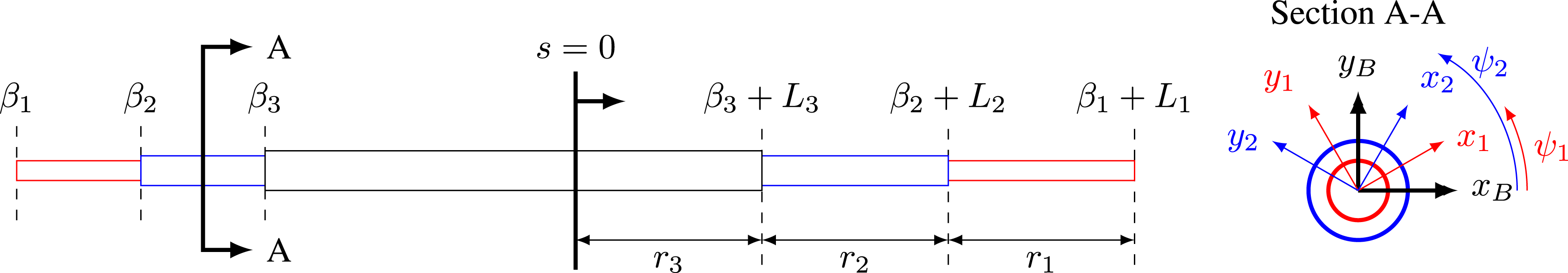

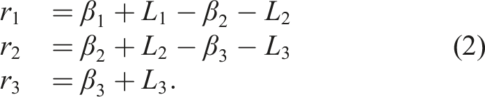
The inner, middle, and outer tubes correspond to subscripts 1, 2, and 3, respectively, and ${\psi }_i(s) = {\psi }_{is}$ for compactness.

We use tip angles ψ _L as joint variables here because they correspond to a unique configuration of the robot, which enables us to solve a single differential equation to determine the shape of the robot, rather than performing a shooting method on the differential equation, as would be needed if base angles were used. Note that after solving the initial value problem differential equation, the base angles ψ _β are known and can be commanded to the actuators. Furthermore, if base angles are used, the robot’s configuration is not guaranteed to be uniquely specified, and can depend on actuation history (Hendrick et al. 2015; Gilbert et al. 2016a).

Throughout this paper, we use the elastic stability measure proposed in (Gilbert et al. 2016b). We give this stability measure the symbol $\mathbb{S}$ , a scalar that is positive when the robot configuration is stable and negative when the robot configuration is unstable. Physically, the robot goes unstable when there is a direction in the solution space in which the robot can move to a lower energy state. This is identified mathematically by a negative eigenvalue of the second variation operation of the energy functional of the robot’s twist angles. See (Gilbert et al. 2016a) for a complete derivation and evaluation of the metric.

2.2. Redundancy resolution framework

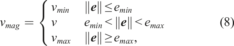
During resolved rates teleoperation, the surgeon commands a desired trajectory, which is converted to a desired task space velocity ${\dot{\mathit{x}}}_d\in {\mathbb{R}}^{m\times 1}$ . The robot’s Jacobian $\mathbf{J}\in {\mathbb{R}}^{m\times n}$ maps instantaneous joint velocities $\dot{\mathit{q}}\in {\mathbb{R}}^{n\times 1}$ to instantaneous task space velocities: $\mathbf{J}\dot{\mathit{q}}={\dot{\mathit{x}}}_d$ . Note that we use the hybrid Jacobian (Murray et al. 1994) throughout this paper, with the desired task space velocity specified in the robot’s base frame coordinates.

To control a concentric tube robot to track a sequence of desired tip coordinates, we use the weighted damped least squares framework (Wampler II 1986), into which we previously incorporated tracking, damping, and joint limits (Burgner et al. 2014). In this work, we use the same tracking, damping, and joint limit goals as Burgner et al.; our contribution to this framework is the addition of instability avoidance and desired stiffness as additional objectives within this algorithm.

The damped least squares framework defines a cost function and applies weights to these potentially competing objectives. The cost function H, using the notation from (Burgner et al. 2014), is given as

$\begin{array}{r}H=\frac{1}{2}({\left(\mathbf{J}\dot{\mathit{q}}-{\dot{x}}_d\right)}^T{\mathbf{W}}_0\left(\mathbf{J}\dot{\mathit{q}}-{\dot{x}}_d\right)+\\ \sum _{i=1}^p{\left(\dot{\mathit{q}}-v_i\right)}^T{\mathbf{W}}_i\left(\dot{\mathit{q}}-v_i\right)),\end{array}$

(3)

where W _i are non-negative symmetric weighting matrices. The first term penalizes any $\dot{\mathit{q}}$ which does not follow the surgeon’s command, while subsequent terms can be used to damp high velocities (if v _i is set to zero), to penalize joint configurations that are near joint limits, or to encourage joint velocities in the direction of the gradient v _i of some objective function. The necessary condition for $\dot{\mathit{q}}$ to minimize H is found by setting $\partial H/\partial \dot{\mathit{q}}=0$ , and can be shown to be

$\dot{\mathit{q}}={\left({\mathbf{J}}^{\mathsf{T}}{\mathbf{W}}_0\mathbf{J}+{\displaystyle \sum }_{i=1}^p{\mathbf{W}}_i\right)}^{-1}\left({\mathbf{J}}^{\mathsf{T}}{\mathbf{W}}_0{\dot{\mathit{x}}}_d+{\displaystyle \sum }_{i=1}^p{\mathbf{W}}_i{\mathit{v}}_i\right).$

(4)

In this paper, we will use a cost function and update law with standard tracking, damping, and joint limit avoidance terms that will be augmented with novel instability avoidance and stiffness tuning terms. The cost function is given by

$H=\frac{1}{2}(\underset{\text{Tracking}}{\underbrace{{\left(\mathbf{J}\dot{\mathit{q}}-{\dot{\mathit{x}}}_d\right)}^{\mathsf{T}}{\mathbf{W}}_0\left(\mathbf{J}\dot{\mathit{q}}-{\dot{\mathit{x}}}_d\right)}}+\underset{\text{Damping}}{\underbrace{{\dot{\mathit{q}}}^{\mathsf{T}}{\mathbf{W}}_D\dot{\mathit{q}}}}+\underset{\text{Joint} \text{Limit} \text{Avoidance}}{\underbrace{{\dot{\mathit{q}}}^{\mathsf{T}}{\mathbf{W}}_J\dot{\mathit{q}}}}+\underset{\text{Secondary} \text{Goal}}{\underbrace{{\left(\dot{\mathit{q}}-{\mathbf{v}}_i\right)}^{\mathsf{T}}{\mathbf{W}}_i\left(\dot{\mathit{q}}-{\mathbf{v}}_i\right)}}),$

(5)

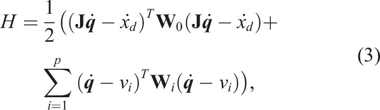
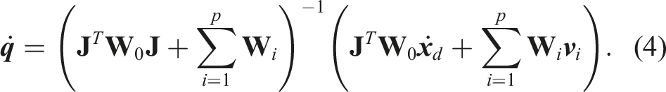
which can again by minimized by setting $\partial H/\partial \dot{\mathit{q}}=0$ . The resulting instantaneous joint velocity vector that minimizes H is

$\begin{array}{l}\dot{\mathit{q}}={\left({\mathbf{J}}^{\mathsf{T}}{\mathbf{W}}_0\mathbf{J}+{\mathbf{W}}_D+{\mathbf{W}}_J\left(\mathit{q}\right)+{\mathbf{W}}_{\mathbf{i}}\left(\mathit{q}\right)\right)}^{-1}\\ \left({\mathbf{J}}^{\mathsf{T}}{\mathbf{W}}_0{\dot{\mathit{x}}}_d+{\mathbf{W}}_{\mathbf{i}}\left(\mathit{q}\right){\mathit{v}}_i\right).\end{array}$

(6)

We will examine each term in this cost function and resulting update law in subsequent subsections. In particular, the instability avoidance and stiffness tuning terms are an important contribution of this work. The gains used in the algorithm are summarized in Table 1.

Table 1.

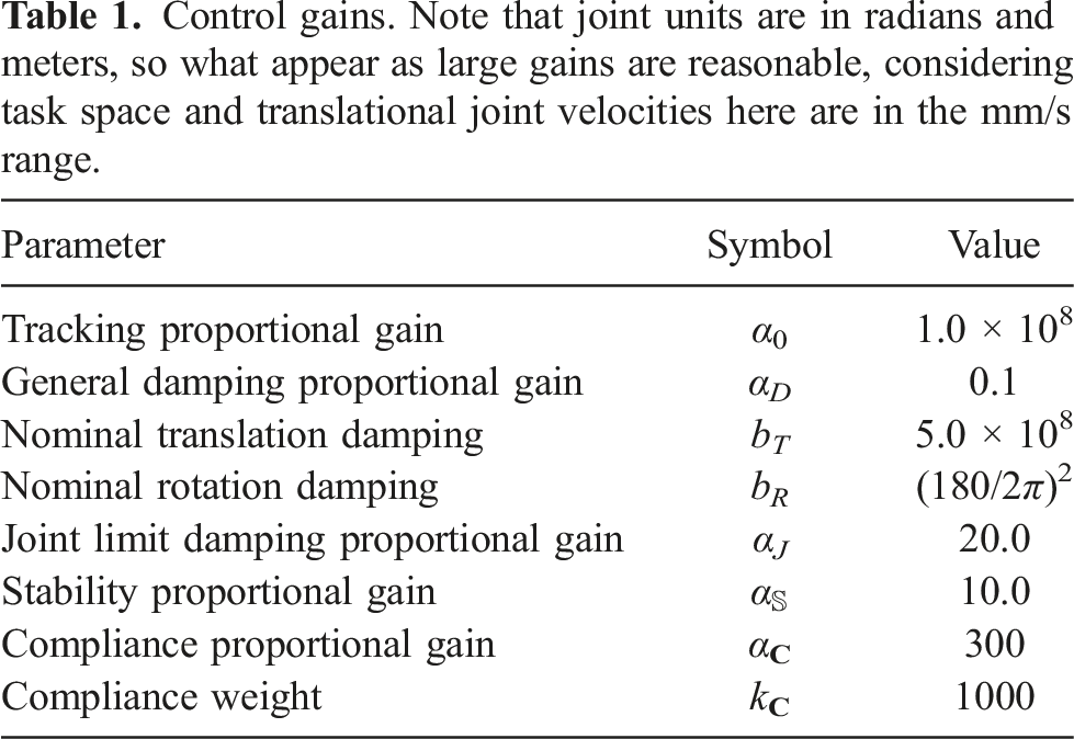
Control gains. Note that joint units are in radians and meters, so what appear as large gains are reasonable, considering task space and translational joint velocities here are in the mm/s range.

Parameter	Symbol	Value
Tracking proportional gain	α 0	1.0 × 108
General damping proportional gain	α D	0.1
Nominal translation damping	b T	5.0 × 108
Nominal rotation damping	b R	(180/2π)2
Joint limit damping proportional gain	α J	20.0
Stability proportional gain	${\alpha }_{\mathbb{S}}$	10.0
Compliance proportional gain	α C	300
Compliance weight	k C	1000

2.2.1. Tracking

The first term in the cost function (5) penalizes joint velocities $\dot{\mathit{q}}$ that differ from those specified by the surgeon. The desired task space velocity is calculated using the current tip position p _tip given by the kinematic model and the desired tip position p _des from the surgeon interface:

$\begin{array}{ll}\mathit{e}& ={\mathit{p}}_{des}-{\mathit{p}}_{tip}\\ {\dot{\mathit{x}}}_{des}& =v_{mag}\frac{\mathit{e}}{\Vert \mathit{e}\Vert }\end{array}$

(7)

where v _mag is a piecewise continuous function of the magnitude of e given by

$v_{mag}=\{\begin{array}{ll}{v}_{\mathit{min}}& \Vert \mathit{e}\Vert \le e_{\mathit{min}}\\ v& e_{\mathit{min}}<\Vert \mathit{e}\Vert <e_{\mathit{max}}\\ v_{\mathit{max}}& \Vert \mathit{e}\Vert \ge e_{\mathit{max}},\end{array}$

(8)

where

$v=\frac{v_{\mathit{max}}-v_{\mathit{min}}}{e_{\mathit{max}}-e_{\mathit{min}}}\left(\Vert \mathbf{e}\Vert -e_{\mathit{max}}\right)+v_{\mathit{max}}.$

(9)

We also set a converged radius ρ, so that if ‖ e ‖ < ρ, ${\dot{\mathit{x}}}_{des}=0$ . The control gains for selecting the task space velocity are found in Table 2. The tracking weighting matrix is defined as

${\mathbf{W}}_0={\alpha }_0{\mathbf{I}}_{3\times 3},$

(10)

where α₀ is a proportional tracking gain. Note that if tracking in a certain direction is more important than others, the elements of this weighting matrix could be adjusted accordingly by using a higher gain for these directions.

Table 2.

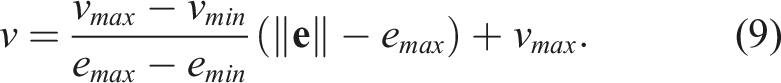
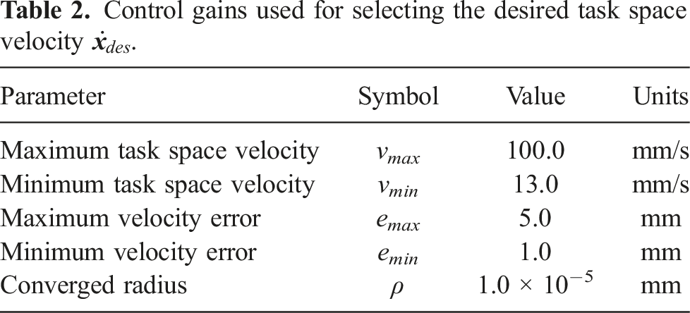
Control gains used for selecting the desired task space velocity ${\dot{\mathit{x}}}_{des}$ .

Parameter	Symbol	Value	Units
Maximum task space velocity	v max	100.0	mm/s
Minimum task space velocity	v min	13.0	mm/s
Maximum velocity error	e max	5.0	mm
Minimum velocity error	e min	1.0	mm
Converged radius	ρ	1.0 × 10−5	mm

2.2.2. Damping

The second term in the cost function (5) penalizes high joint velocities 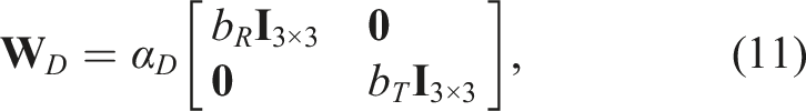$\dot{\mathit{q}}$ , adding numerical damping. The damping term has a weighting matrix defined by

${\mathbf{W}}_D={\alpha }_D\left[\begin{array}{ll}{b}_R{\mathbf{I}}_{3\times 3}& \mathbf{0}\\ \mathbf{0}& b_T{\mathbf{I}}_{3\times 3}\end{array}\right],$

(11)

where α _D is an overall proportional damping gain, b _R is a rotational damping gain, and b _T is a translational damping gain. We distinguish b _R and b _T due to the different rotation and translation units.

2.2.3. Joint limit avoidance

The third term in the cost function (5) penalizes joint velocities 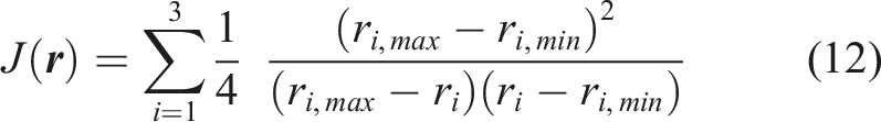$\dot{\mathit{q}}$ that violate joint limits. Here, we define joint limits based on the exposed length of each tube. For each tube, we define a minimum and maximum exposed length, r_i, min and r_i, max. In the simulations that follow, we make the choice to prevent a given tube from being retracted beyond the tip of the tube surrounding it, meaning that all r_i, min must be greater than zero. Note that this joint limit definition could be relaxed if desired; it is not an intrinsic part of the algorithm. Specifically, we set all r_i, min to 1 mm and all r_i, max to 40 mm for the simulation studies. For the robotic experiments, we define the maximum limits based on the robot actuation unit travel limits. To avoid these joint limits, we define a joint limit penalty function as

$J\left(\mathit{r}\right)={\displaystyle \sum }_{i=1}^3\frac{1}{4}\frac{{\left(r_{i,\mathit{max}}-r_{i,\mathit{min}}\right)}^2}{\left(r_{i,\mathit{max}}-r_i\right)\left(r_i-r_{i,\mathit{min}}\right)}$

(12)

which was inspired by results in (Chan and Dubey 1995). We then define a weighting matrix as,

${\mathbf{W}}_J\left(\mathit{q}\right)={\alpha }_J\text{diag}\left(1+\left|\nabla J_{\mathit{q}}\right|\right)$

(13)

where

$\nabla J_{\mathit{q}}=\left[\begin{array}{llllll}0& 0& 0& J_{r_1}& J_{r_2}& J_{r_3}\end{array}\right]$

(14)

$J_{r_i}=\partial J/\partial r_i$ , and α _J is a proportional joint limit avoidance gain. We do not enforce rotational joint limits, so the first three elements of ∇J _q are zero. With this strategy, the joint limit avoidance term dominates the cost function when a joint value r _i approaches its limits.

2.2.4. Instability avoidance

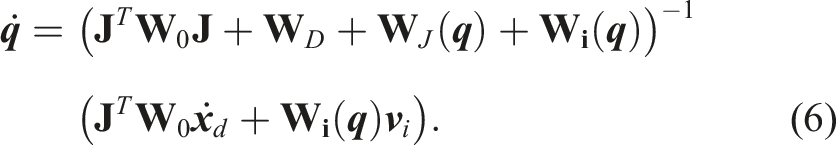
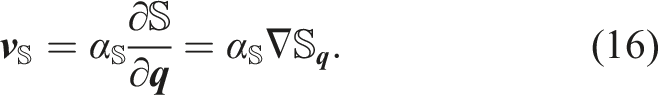
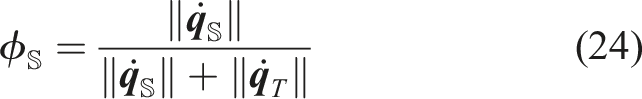
When resolving redundancy to avoid elastic instability, the final term in the cost function (5) (i.e., the secondary goal) is designed to dominate the cost function when the robot configuration approaches instability as given by the metric 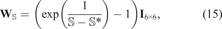$\mathbb{S}$ , derived in (Gilbert et al. 2016a). We define an instability avoidance weighting matrix as

${\mathbf{W}}_{\mathbb{S}}=\left(\exp \left(\frac{1}{\mathbb{S}-\mathbb{S}*}\right)-1\right){\mathbf{I}}_{6\times 6},$

(15)

in which each diagonal element approaches infinity as $\mathbb{S}$ approaches the stability threshold $\mathbb{S}*$ . In such cases, we want the update law to command joint velocities that move the robot away from unstable configurations. To do so, we define

${\mathit{v}}_{\mathbb{S}}={\alpha }_{\mathbb{S}}\frac{\partial \mathbb{S}}{\partial \mathit{q}}={\alpha }_{\mathbb{S}}\nabla {\mathbb{S}}_{\mathit{q}}.$

(16)

By choosing the proportional gain ${\alpha }_{\mathbb{S}}>0$ , the system will ascend the stability gradient when the instability avoidance term dominates the cost function, moving the robot to a more stable configuration. We numerically compute the stability gradient $\nabla {\mathbb{S}}_{\mathit{q}}$ using centered finite difference (translational step = 0.01 mm, rotational step = 0.05°). When computing this gradient, we take advantage of our choice of joint variables (see Sec. 2.1). Controlling tip angles and solving the kinematic model as an initial value problem with a single differential equation improves computational speed.

The instability avoidance weighting matrix (15) is designed such it does not impact the control law (6) when the robot’s stability $\mathbb{S}$ is far from the stability threshold $\mathbb{S}*$ . In these cases, the diagonal elements of ${\mathbf{W}}_{\mathbb{S}}$ are nearly zero. The closer the stability metric to the threshold, the more the instability avoidance term dominates the control law, causing the controller to steer the robot toward more stable configurations. This approach does not seek to continually maximize stability; rather, instability avoidance is only employed when necessary, allowing the controller to use as much of the stable configuration space as possible. Note that when this term is used in the remainder of the paper, we will refer to (6) as the “instability avoidance control law.”

2.2.5. Stiffness tuning

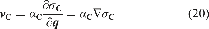
When resolving redundancy to tune stiffness, we set a stiffness-based secondary goal in the cost function (5). To accomplish this, we make use of the concentric tube robot’s compliance matrix $\mathbf{C}\in {\mathbb{R}}^{6\times 6}$ , which maps a tip wrench $\mathit{\omega }\in {\mathbb{R}}^{6\times 1}$ to a tip deflection $\mathit{\delta }\in {\mathbb{R}}^{6\times 1}$ as $\mathbf{C}\mathit{\omega } = \mathit{\delta }$ (see (Rucker and Webster III 2011)). In surgical scenarios, it is common for the robot to experience tip loads; therefore, we will utilize C _fp , which is the top left 3 × 3 submatrix of C that maps a force f to a position deflection δ _p .

While a variety of stiffness objectives can be defined based on this tip stiffness matrix, in the simulations that follow we simply use the maximum singular value of C _fp , for which we use the symbol σ _C . More precisely, we have that

${\mathbf{C}}_{\mathit{f}\mathit{p}}=\mathbf{U}\mathbf{\Sigma }{\mathbf{V}}^{\mathsf{T}}$

(17)

and define σ _C as

${\sigma }_{\mathbf{C}}\triangleq \max \left(\text{diag}\left(\mathbf{\Sigma }\right)\right).$

(18)

This means that when σ _C is maximized, the system will attempt to achieve configurations with maximal compliance in its most compliant direction. On the other hand, when σ _C is minimized, the system will attempt to achieve configurations with minimal compliance in its most compliant direction. Alternative metrics for stiffness tuning include minimizing tip deflection (if the applied load vector is known) or optimizing stiffness in a particular direction (e.g., axial or lateral stiffness, which could be beneficial for different applications).

We define a compliance weighting matrix as

${\mathbf{W}}_{\mathbf{C}}=k_{\mathbf{C}}{\mathbf{I}}_{6\times 6}.$

(19)

In order to maximize or minimize σ _C , we define a joint space velocity vector v _C as

${\mathit{v}}_{\mathbf{C}}={\alpha }_{\mathbf{C}}\frac{\partial {\sigma }_{\mathbf{C}}}{\partial \mathit{q}}={\alpha }_{\mathbf{C}}\nabla {\sigma }_{\mathbf{C}}$

(20)

which points along the positive gradient of σ _C if the user defines α _C > 0 and along the negative gradient of σ _C if the user defines α _C < 0. This will command joint velocities that make the robot more (or less) compliant in its most compliant direction. We compute ∂σ _C /∂ q numerically using the same centered finite difference parameters as Sec. 2.2.4. Unlike the instability avoidance term in the control law, which changes in magnitude based on proximity to the stability threshold, the compliance optimization term seeks to always move the robot into more (or less) compliant configurations due to the constant gain k _C used to compute the weighting matrix W _C . Note that when this term is used in the paper, we will refer (6) as the “stiffness tuning control law.”

3. Simulations

We first tested our redundancy resolution algorithm for both instability avoidance and stiffness tuning in simulation to verify its effectiveness, analyze its impact on the robot’s behavior, and tune the control gains. This section describes first the instability avoidance simulations, followed by the stiffness tuning simulations.

3.1. Instability avoidance simulations

To test our elastic stability-aware redundancy resolution algorithm, we simulated the real-time control of a three-tube concentric tube robot made of superelastic nitinol tubes (E = 50 GPa, ν = 0.33, see Table 3 for tube dimensions) along a desired trajectory. In this simulation, we used the gain parameters given in Tables 1 and 2, as well as a minimum stability threshold of $\mathbb{S}*=0$ .

Table 3.

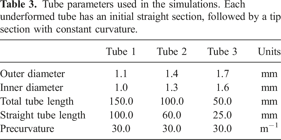
Tube parameters used in the simulations. Each underformed tube has an initial straight section, followed by a tip section with constant curvature.

	Tube 1	Tube 2	Tube 3	Units
Outer diameter	1.1	1.4	1.7	mm
Inner diameter	1.0	1.3	1.6	mm
Total tube length	150.0	100.0	50.0	mm
Straight tube length	100.0	60.0	25.0	mm
Precurvature	30.0	30.0	30.0	m−1

3.1.1. Desired trajectory

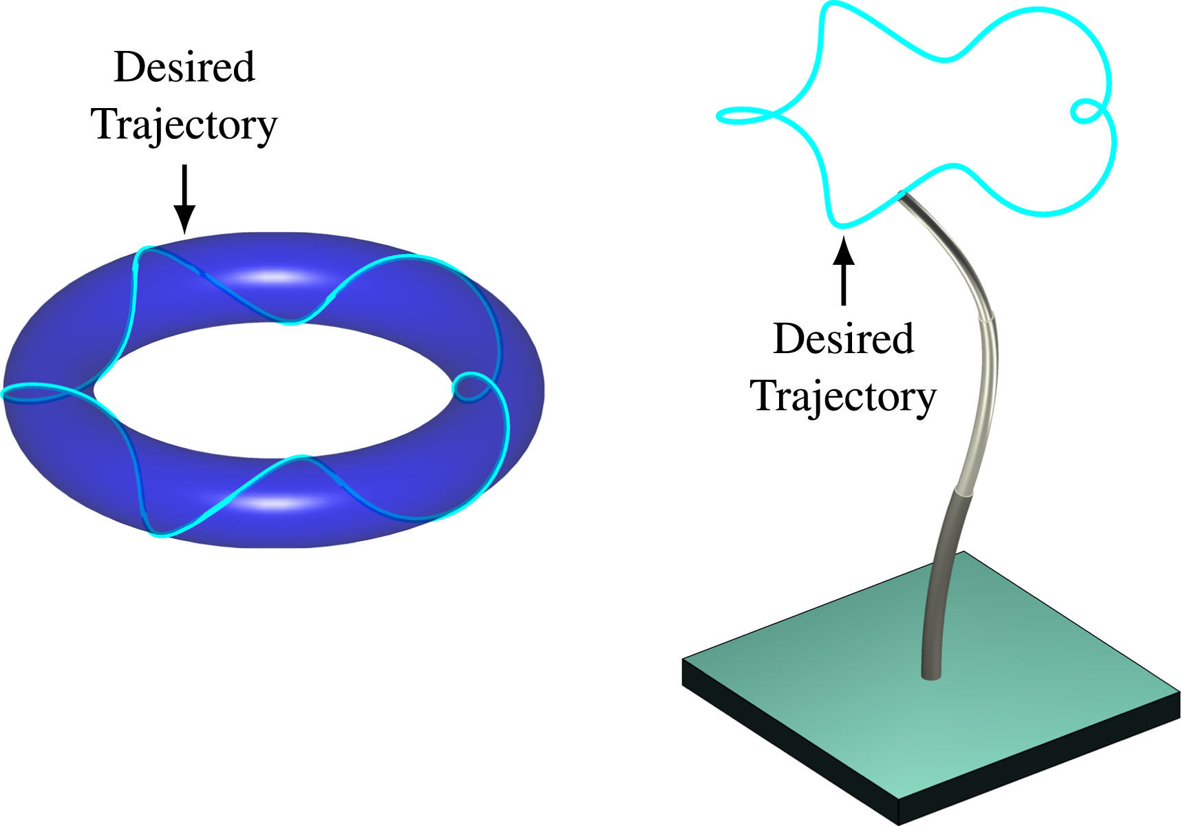
During teleoperation, the desired input velocities are those commanded by the surgeon. Here, to create an example trajectory to use in simulation, we chose a helix wrapping around a torus, as shown in Figure 3. The equations defining the desired tip position were

${\mathit{p}}_{des}=\left[\begin{array}{l}\left(R+r\cos \left(N_T\theta \right)\right)\cos \left(\theta \right)\\ \left(R+r\cos \left(N_T\theta \right)\right)\sin \left(\theta \right)\\ r\sin \left(N_T\theta \right)+z_{off}\end{array}\right],$

(21)

where the torus’ major radius (R) was 15.0 mm, its minor radius (r) was 3.0 mm, the number of helix turns (N _T ) was 5, the offset from the x-y plane (z _off ) was 55.0 mm, and θ ∈ [0, 2π). The robot’s home position was given by ψ _L = 0 and r₁ = r₂ = r₃ = 20 mm. We used a total simulation time of 10 s with a step time of 5 ms and implemented a standard resolved rates scheme in which the desired tip velocities were calculated using the error vector between the current position and desired position at each time step.

Figure 3.

(Left) Desired trajectory of a helix wrapping around a torus. (Right) Simulated concentric tube robot following the desired trajectory.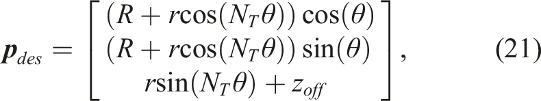

3.1.2. Simulation results

We performed the simulation both with (the “stability-aware” case) and without (the “stability-unaware” case) the instability avoidance term included in the cost function and control law. In Figure 4(a), we show the stability metric and tracking error throughout the entire trajectory for the stability-unaware case. Due to the high curvature of the tubes and the commanded trajectory, the robot snaps twice. However, the controller has no knowledge of this instability nor does it have a way to avoid it. Based purely on the kinematic model, the robot appears to be tracking well from the controller’s perspective. However, the physical robot is in a different local minimum energy solution than the local minimum energy solution assumed by the controller, due to the uncontrolled snapping. As soon as the stability metric first crosses to $\mathbb{S}<0$ , the robot snaps to a configuration far away and tracking is lost.

Figure 4.

(a) When the control law is stability-unaware, the robot’s stability crosses to 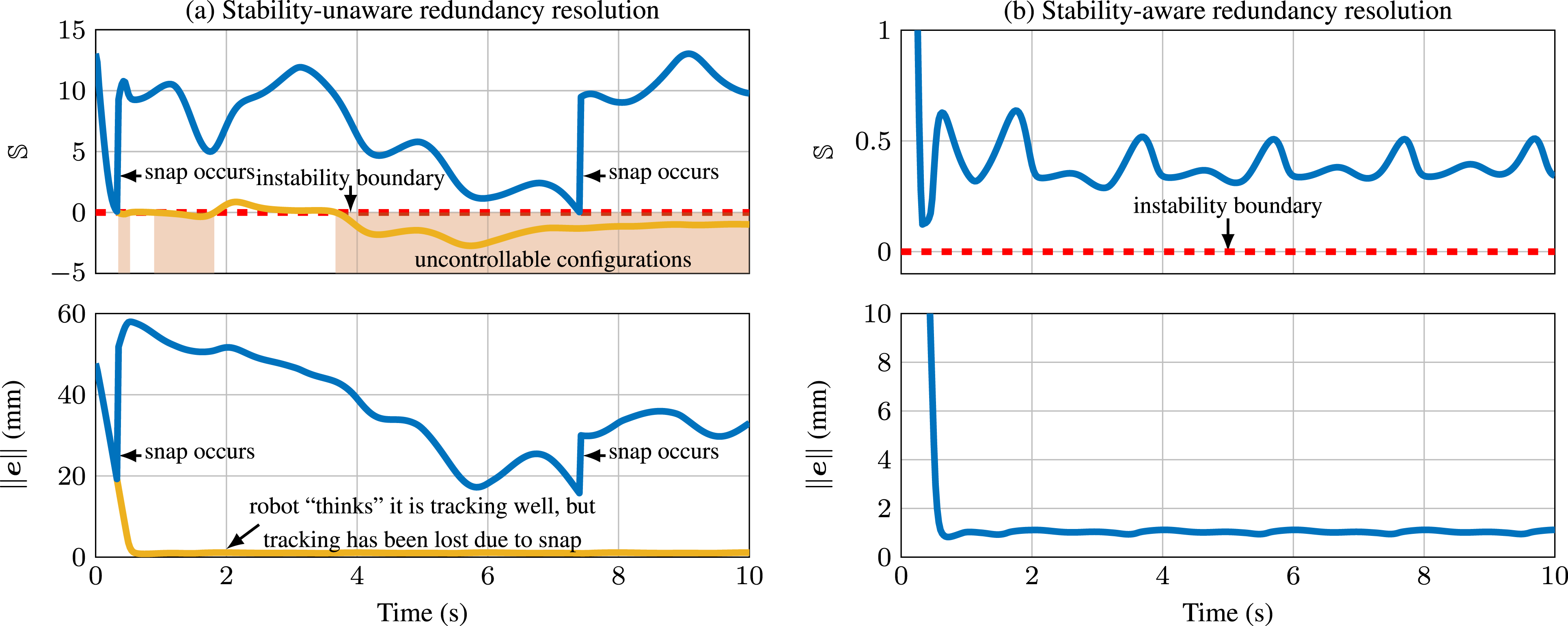$\mathbb{S}<0$ and it snaps to a new configuration. Based on the kinematic model alone, tracking appears to be good, but tracking of the physical robot has been lost. (b) When the controller is stability-aware, the entire trajectory is stabilized. When $\mathbb{S}$ approaches zero, the robot moves away from the unstable configuration while still tracking the trajectory.

Figure 4(b) shows that using the instability avoidance control law enables the robot to avoid instabilities while maintaining good tracking ( ∼1 mm) in task space. Note that the error along the chosen trajectory is due to the dynamic trajectory and high damping; the error quickly reduces to $<$ 0.01 mm when regulating a constant desired tip position. At the beginning of the trajectory, stability moves toward zero, but unlike Figure  4(a), the instability avoidance term causes the robot to move to a more stable configuration while continuing to track the desired trajectory.

3.1.3. Computing the robot’s post-snap configuration

In order to generate the simulated unstable robot trajectory, we calculated the new physical configuration of the robot in cases where the robot snaps. This was necessary for finding the results of Figure 4(a). The key idea behind this problem is that, when the robot is in an unstable configuration, there are multiple configurations in model space (and therefore multiple sets of tip angles ψ _L ) corresponding to the same base rotational angles ψ _β . When the robot snaps, the current tip angles are unstable, and the physical solution must be found. To find the new post-snap configuration, one must search the tip angle space for a configuration corresponding to the same base angles ψ _β . Note that the relative tube angles affect stability, not the absolute angles, so the search for the new configuration is done in the relative angle space and then converted back to absolute angles. We define the relative joint angles as ${\theta }_i(s) = {\psi }_i(s) - {\psi }_1(s)$ .

When the stability of the robot in the simulation goes to 0, we use MATLAB’s fzero function to find the exact relative tube angles θ _L,unstable at the edge of the unstable configuration space. This point is shown by the “before snap” points in Figure 5. Once this unstable configuration is found, we calculate the unique relative base angles θ _β using the kinematic model. Then, we use MATLAB’s fsolve function to find another set of relative tip angles θ _L,stable that produce the same relative base angles as the unstable solution.

Figure 5.

These plots show the relative tip angle configuration space of the simulated three-tube concentric tube robot. The colormap depicts the stability measure $\mathbb{S}$ , truncated from 0 to 1. The red line is the boundary of the unstable region. When the robot hits this boundary at the “before snap” point , it snaps. The new configuration it reaches after the snap can be found by searching the configuration space for a set of relative tip angles that produces the same relative base angles at the actuators (“after snap” points ). Note that the shape of the unstable region can change substantially based on tube translation variables.

Because the relative joint space is wrapped from 0 to 2π radians we must convert the new relative tip angles to absolute angles. To do so, we first assume a configuration of ${\mathit{\psi }}_{L,guess}={\left[0,{\theta }_{2L,stable},{\theta }_{3L,stable}\right]}^{\mathsf{T}}$ . Solving the kinematic model returns absolute base angles that have the same relative angles but are offset from the original absolute base angles by Δ ψ . We then add this offset to the tip angle guess to get the new, stable configuration:

${\mathit{\psi }}_{L,stable}={\left[\begin{array}{lll}0& {\theta }_{2L,stable}& {\theta }_{3L,stable}\end{array}\right]}^{\mathsf{T}}+\mathrm{\Delta }\mathit{\psi }.$

(22)

The new robot configuration is shown by the “after snap” points in Figure 5. This approach could potentially be used in a physical system to “recover” tracking should a snap occur.

3.1.4. Effect of instability avoidance

When using the weighted damped least squares approach for redundancy resolution, there are several interacting variables (damping, joint limit avoidance, tracking, and instability avoidance) which interact in a nonlinear manner. Selecting gains can be challenging and the performance of the algorithm can be sensitive to these gain selections. There was one analysis tool that proved particularly useful towards selecting these gains. 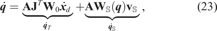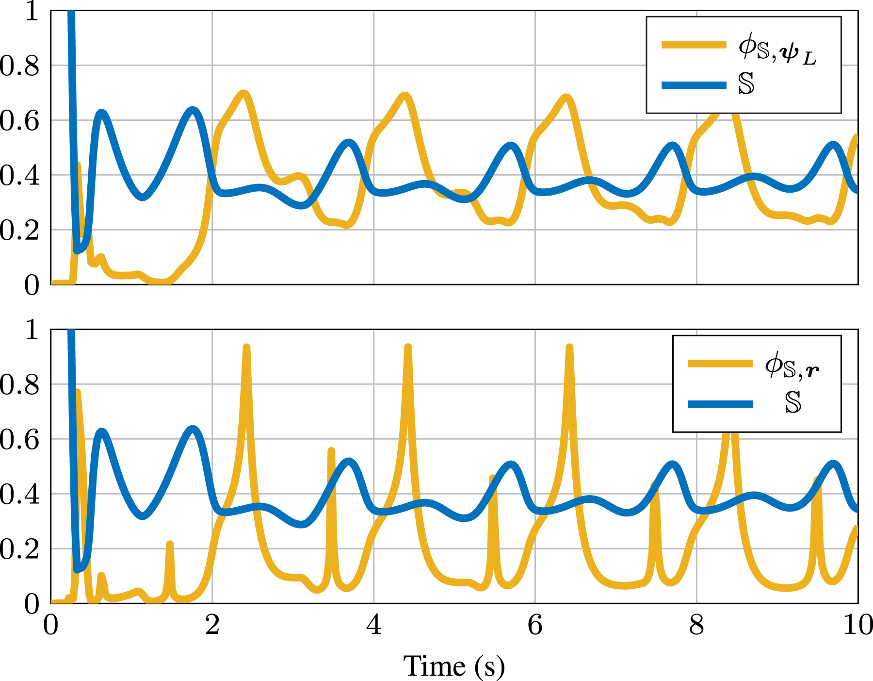If we define the 6 × 6 inverted matrix from (6) as A, then we can re-express this update law as

$\dot{\mathit{q}}=\underset{{\stackrel{.}{\mathit{q}}}_T}{\underbrace{\mathbf{A}{\mathbf{J}}^{\mathsf{T}}{\mathbf{W}}_0{\dot{\mathit{x}}}_d}}+\underset{{\stackrel{.}{\mathit{q}}}_{\mathbb{S}}}{\underbrace{\mathbf{A}{\mathbf{W}}_{\mathbb{S}}\left(\mathit{q}\right){\mathbf{v}}_{\mathbb{S}}}},$

(23)

and it becomes clear that the joint velocity ${\dot{\mathit{q}}}_T$ is related to tracking, and the joint velocity ${\dot{\mathit{q}}}_{\mathbb{S}}$ is related to instability avoidance. We can compare the norm of these two competing joint velocities to better understand which term is dominating the simulation. Figure 6 shows the relative norm of these joint velocities, or

${\varphi }_{\mathbb{S}}=\frac{\Vert {\dot{\mathit{q}}}_{\mathbb{S}}\Vert }{\Vert {\dot{\mathit{q}}}_{\mathbb{S}}\Vert +\Vert {\dot{\mathit{q}}}_T\Vert }$

(24)

for both rotational $\left({\mathit{\varphi }}_{\mathbb{S},{\mathbf{\psi }}_{\mathit{L}}}\right)$ and translational $\left({\mathit{\varphi }}_{\mathbb{S},\mathit{r}}\right)$ joint velocities for the simulation. As is clear from the figure, when $\mathbb{S}$ is low, the effect of ${\dot{\mathit{q}}}_{\mathbb{S}}$ becomes more prominent. In addition, there appears to be an oscillating exchange of control priority from tracking to instability avoidance.

Figure 6.

(Top) ${\varphi }_{\mathbb{S},{\mathbf{\psi }}_L}$ and $\mathbb{S}$ in time. When stability is low, stabilizing rotational joint velocities become more prominent. (Bottom) ${\varphi }_{\mathbb{S},\mathbf{r}}$ and $\mathbb{S}$ in time. When stabilility is low, there are short bursts of stabilizing translational joint velocities.

3.1.5. Effect of Stability Threshold

We explored the effect of the stability threshold $\mathbb{S}*$ on the robot’s behavior. We performed the trajectory-following simulation with $\mathbb{S}*$ chosen as 0.0, 0.1, 0.2, and 0.3. The results of these simulations are shown in Figure 7. In each case, the controller tracks well and does not violate the stability threshold. As can be seen in Figure 7(Top), the stability trajectories are nearly identical and only differ by an offset in $\mathbb{S}$ . The initial tracking response time is slower for higher values of $\mathbb{S}*$ , as shown in Figure 7(Bottom).

Figure 7.

(Top) The stability metric 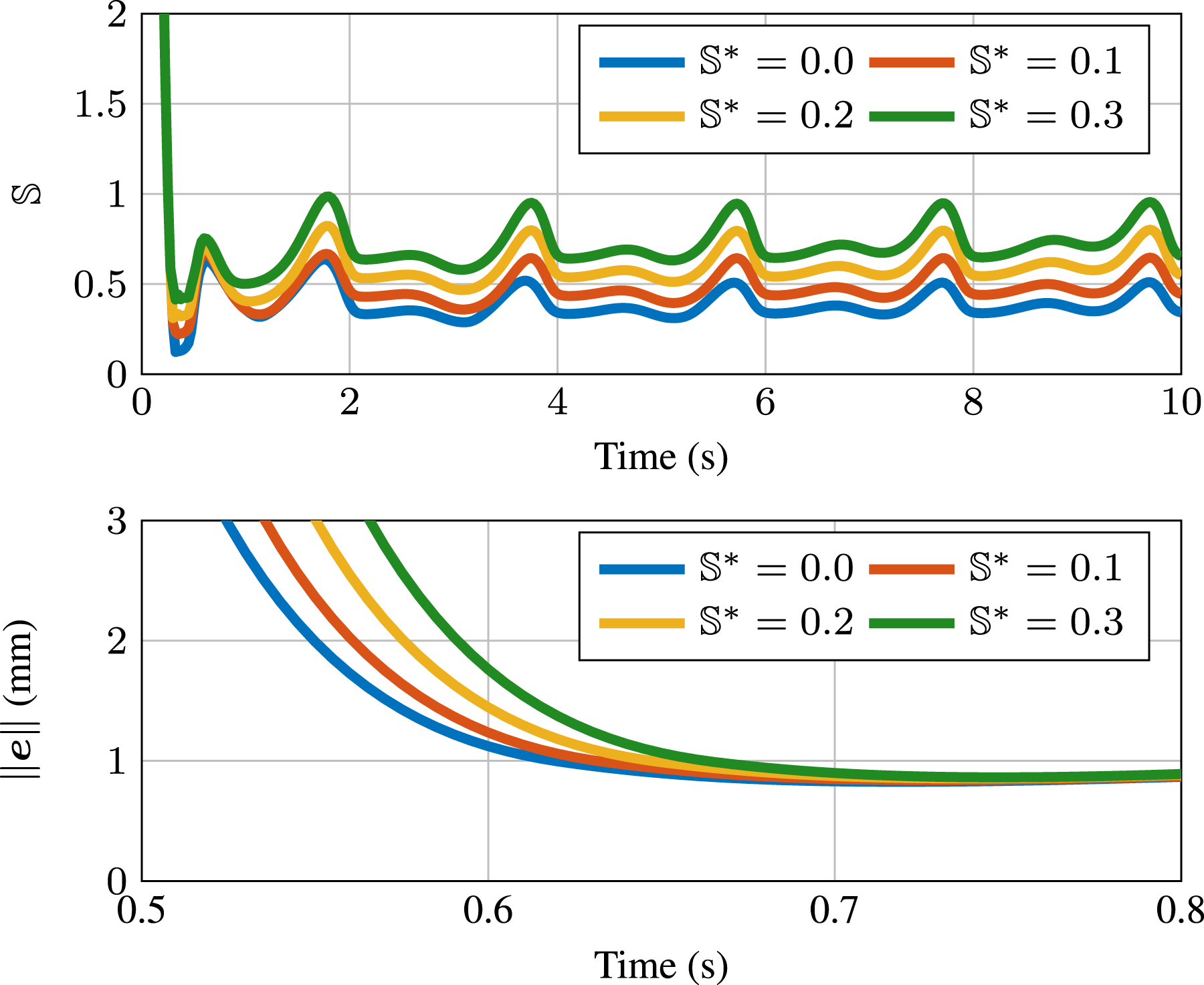$\mathbb{S}$ in time for varying choices of $\mathbb{S}*$ . (Bottom) The tracking error in time for varying choices of $\mathbb{S}*$ . Note that the time axis is only 0.3 s. The tracking response time is correlated with the choice of $\mathbb{S}*$ .

3.2. Stiffness tuning simulations

To test our stiffness tuning redundancy resolution algorithm, we simulated the real-time control of a three-tube concentric tube robot. For this simulation, we used tubes of the same dimensions as Table 3 with curvatures of 10, 12, and 22 m⁻¹ for tubes 1, 2, and 3, respectively.

3.2.1 Stiffness tuning with trajectory following

First, we optimized σ _C while the robot follows the torus trajectory given by (21). The results for this redundancy resolution controller are shown in Figure 8. The first panel depicts σ _C throughout the trajectory with α _C set to 300 (maximize σ _C ), −300 (minimize σ _C ), and 0 (nominal performance). The second panel shows the difference in performance when maximizing or minimizing σ _C . This shows that the redundancy resolution algorithm is capable of commanding a robot configuration that is nearly four times more compliant (in its most compliant direction) than the least compliant case. The third panel shows the tracking error in task space is similar and small for each case (∼1 mm).

Figure 8.

(Top) Trajectories of the compliance metric σ _C following the path described in (21) with the tubes from Table 3. For the nominal trajectory, we utilize the control law from (4), for the maximum compliance trajectory, we utilize the stiffness tuning update law from (6) with α _C = 300, and the same law for the minimum compliance trajectory with α _C = −300. (Middle) The ratio of σ _C in the maximum compliance trajectory to σ _C in the minimum compliance trajectory. The manipulator becomes nearly four times more compliant by the end of the trajectory, which is likely to be significant in a surgical scenario. (Bottom) All three trajectories have very similar tracking performance.

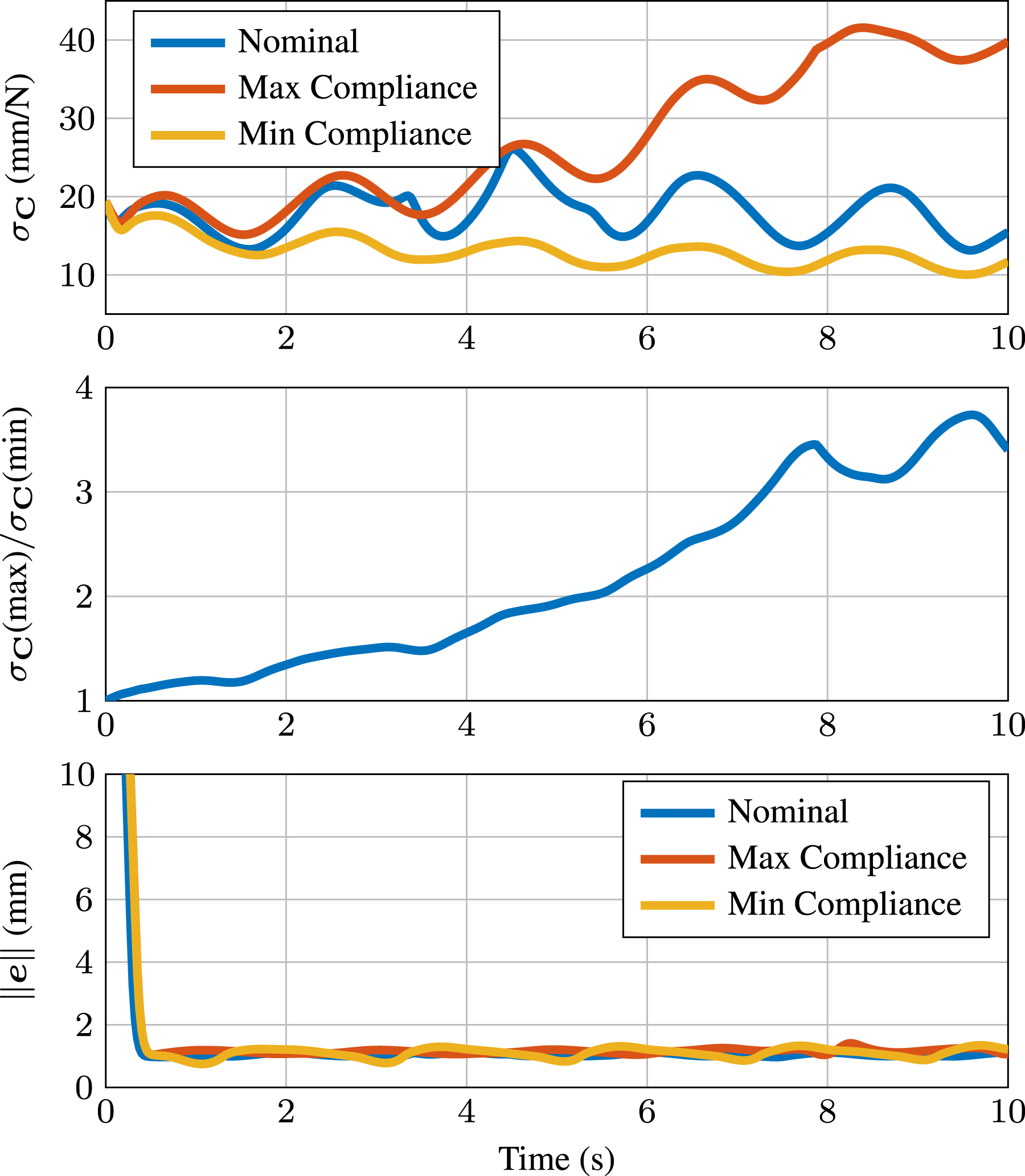
It is likely this difference in compliance would be apparent to a surgeon. It has been shown that the peak forces during minimally invasive surgery are around 2 N for suturing skin, around 1 N for suturing muscle, and typically less than 0.5 N for suturing liver tissue (Peirs et al. 2004). The forces during other tissue interactions (i.e. not driving needles) are typically much less than these. As a specific example of the potential utility of this control law, consider a 0.5 N force on the tip of the concentric tube manipulator investigated here. In maximum compliance mode, this could generate a deflection of up to 20 mm, and in minimum compliance mode, this would generate a deflection as small as 5 mm. This could very well be the difference between being able to drive the needle and not drive the needle.

3.2.2. Stiffness tuning with position regulation

Next, we sought to maximize or minimize σ _C while keeping the tip position of the robot at a fixed position in space, which illustrates the degree of stiffness tuning self-motion. We commanded a static tip position at $\mathit{p}={\left[\mathrm{1,1,55}\right]}^{\mathsf{T}}$ mm, which is near the center of the robot’s workspace. The simulation lasted for 40 seconds, where every 10 seconds we changed the goal from maximizing (α _C > 0) to minimizing (α _C < 0) σ _C , or vice versa. This is shown in the first panel of Figure 9.

Figure 9.

These plots show the manipulator tracking a single point at all times. Every 10 seconds, the system switches between maximizing and minimizing the compliance metric. Notice that the inner tube extends and the outer tube retracts to maximize compliance, and the opposite happens to minimize compliance. The tracking error (not shown) goes below 0.1 mm in 0.5 s and remains there.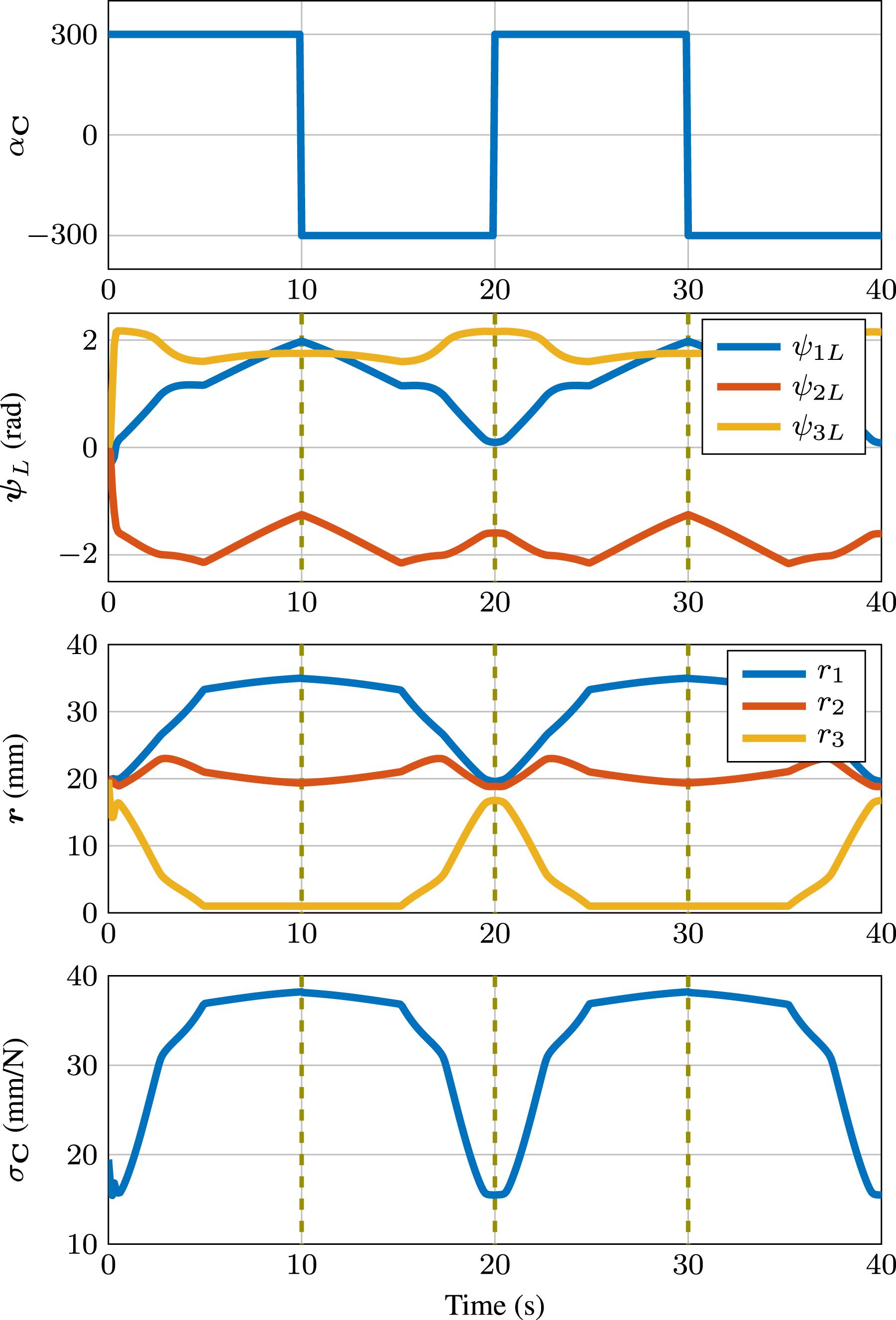

The second and third panels of Figure 9 show the configuration variable paths that move the robot from compliant configurations to stiff configurations, and vice versa. The translational joint values shown in the third panel make intuitive sense: when maximizing σ _C , the outer tube nearly fully retracts (r₃ approaches 0 mm), meaning that the exposed length of the robot is almost entirely made up of the middle and inner tubes, which are more flexible. The fourth panel of Figure 9 shows σ _C throughout the simulation as it is clearly maximized and minimized according to α _C . Also, note that the error is not plotted here, but quickly approaches ∼0.1 mm and remains there throughout the trajectory.

4. Experiments

After exploring the ability of the controller to avoid instabilities and tune stiffness in simulation, we conducted experiments to verify performance on physical hardware. This is an important contribution of this paper, since previous investigations of controllers including stability metrics have been solely in simulation.

4.1. Instability avoidance experiments

To evaluate the elastic stability-aware redundancy resolution algorithm on robotic hardware, we performed a series of experiments using a three-tube concentric tube robot. The tube dimensions are listed in Table 4. First, we conducted a trajectory following experiment to compare the simulation results to a physical robotic system. Next, we used a teleoperation experiment to demonstrate the use of the redundancy resolution algorithm.

Table 4.

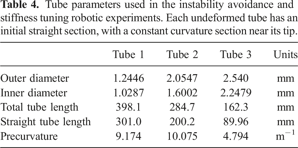
Tube parameters used in the instability avoidance and stiffness tuning robotic experiments. Each undeformed tube has an initial straight section, with a constant curvature section near its tip.

	Tube 1	Tube 2	Tube 3	Units
Outer diameter	1.2446	2.0547	2.540	mm
Inner diameter	1.0287	1.6002	2.2479	mm
Total tube length	398.1	284.7	162.3	mm
Straight tube length	301.0	200.2	89.96	mm
Precurvature	9.174	10.075	4.794	m−1

For both experiments, we used the robotic setup shown in Figure 10. The desired joint velocities are calculated in (6) at each time step of the trajectory following or teleoperation process. The joint values are converted to motor position commands and sent to the six motors that rotate the tubes and translate the tubes along linear slides. Further information on the design and use of this robot can be found in (Burgner et al. 2014; Swaney et al. 2015; Wirz et al. 2015).

Figure 10.

Experimental setup. A magnetic tracking coil was embedded in the tip of the three-tube concentric tube manipulator, which was tracked by the magnetic field generator (Aurora, Northern Digital, Inc.).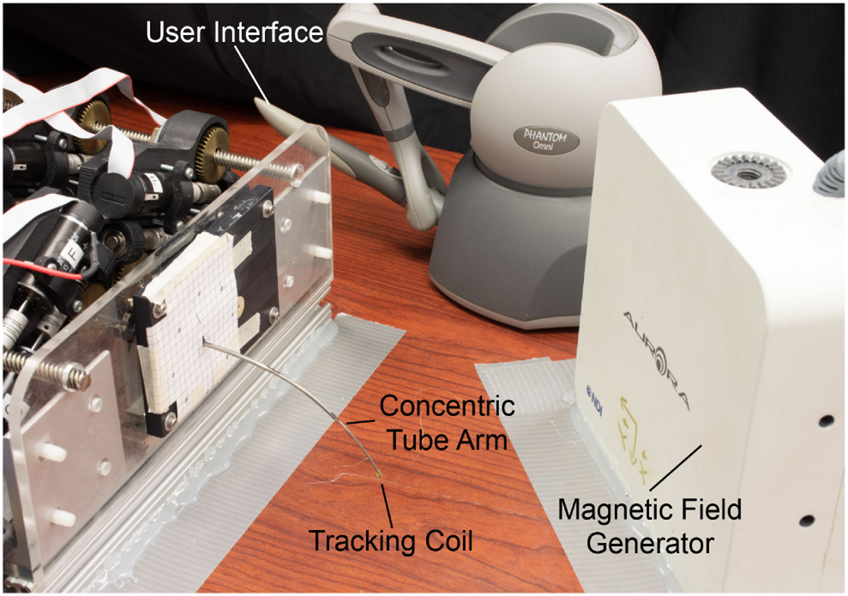

Throughout the experiments, the tip position of the robot was tracked using an electromagnetic tracking coil (Aurora, Northern Digital, Inc.) inserted into the inner tube. The tracker data was used for recording purposes only and was not fed back into the controller (i.e., the controller described in this paper is open loop with respect to the measured tip position). We set the joint limit r_1, min = 10 mm to ensure that the tracking coil was not accidentally dislodged from the inner tube during operation.

After shape-setting the tube curvatures using the procedure described in (Gilbert and Webster III 2016), we measured the resulting curvatures and tube lengths (see Table 4). We then performed a calibration process to register the base pose of the robot (i.e., the exit point s = 0 from the base plate shown in Figure 2) to the tracker frame. We moved the robot joints to 82 configurations and recorded the actuator vectors q and corresponding tip positions in the tracker frame. We used MATLAB’s fmincon function to find the transformation between the tracker frame and the robot base frame by minimizing the total Euclidean error between the tip position transformed into the base frame and the tip position found with the forward kinematics model. The parameters for the optimization routine were the position vector of the transformation, the ZYX Euler rotation angles, and the torsional and bending stiffness of each tube.

4.1.1. Trajectory following experiment

We had the robot follow a helix trajectory similar to the simulations described in Sec. 3.1.1, with the parameters R = 28 mm, r = 12 mm, N _T = 2, and z _off = 110 mm, and a total time of 50 sec. We completed the trajectory 3 times with and without the instability avoidance control law. For each trial, the robot began at the home configuration ψ _L = 0 and r₁ = r₂ = r₃ = 20 mm. From the home configuration, the robot was commanded to the first point of the trajectory (x = 40 mm, y = 0 mm, z = 110 mm) using the instability avoidance control law; this was done so that the robot began at the trajectory in the same configuration whether or not the instability avoidance term would be used for that particular trial. Once the robot tip reached the first point in the trajectory, it stopped for 10 seconds before following the trajectory; here, we jostled the tubes to remove small static frictional effects that may have built up during the transition between the home configuration and the initial trajectory configuration. This again was to ensure uniformity between trials.

During the experiments, the magnetic tracker recorded data at a rate of 40 Hz, and the robot positions were set to update at a loop rate of 125 Hz. The tracking output produced approximately 2000 data points. The tracking output was then transformed from the tracker frame to the robot’s base frame using the calibrated transformation between the two frames. Taking the Euclidean norm between the desired trajectory and sensor data provides the trajectory following error at each time step.

As seen in Figure 11(b), the robot did not snap when using the instability avoidance control law. However, without the control law (Figure 11(a)), the robot exhibited poor tracking and snapped. Snap points are marked with yellow diamonds and the post-snap position is at the tips of the black arrows. Results of this experiment can also be seen in Extension 1 (Table 5).

Figure 11.

These plots show the spatial results of the trajectory following experiment in three planar views (N = 3 trials for each controller). The blue curve is the desired trajectory. (a) Without awareness of elastic stability, the robot snapped while attempting to follow the trajectory. The snapping points are marked with yellow diamonds and the post-snap position is at the tip of the black arrow. (b) With instability avoidance, the robot tracked the trajectory and remained stable.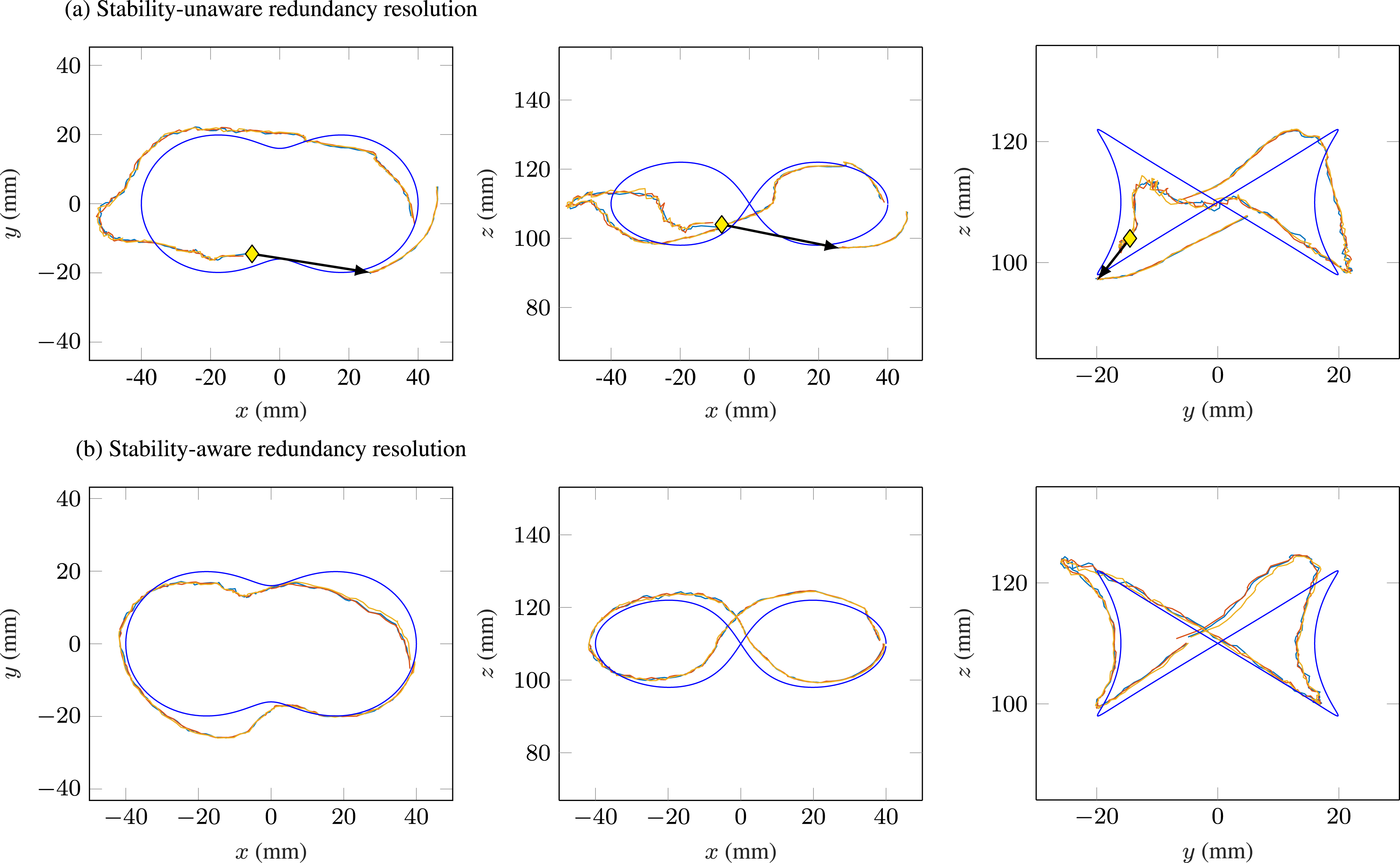

The tracking errors are shown in time in Figure 12. We performed these experiments with a stability threshold $\mathbb{S}*$ of 0.5. The mean error and mean normalized error are shown for the stable and unstable cases as horizontal dashed lines. The mean error for all data across 3 trials with the elastic stability-aware redundancy resolution was 4.18±1.98 mm. When normalized by the extended arclength of the robot at each time step, the mean error was 3.56±1.58%. The mean error with elastic stability-unaware redundancy resolution was 13.84±10.95 mm (11.95±9.58% when normalized by arclength). More importantly, the robot underwent an uncontrolled snap when the controller did not include the instability avoidance term.

Figure 12.

Trajectory following tracking error and normalized error with (a) the stability-unaware controller and (b) the stability-aware controller. Without instability avoidance, the robot underwent an uncontrolled snap. With instability avoidance, the robot both tracked the trajectory and remained stable. The error is shown in blue, and the normalized error is shown in red, while the mean error and mean normalized error are shown with horizontal dashed lines of the same colors.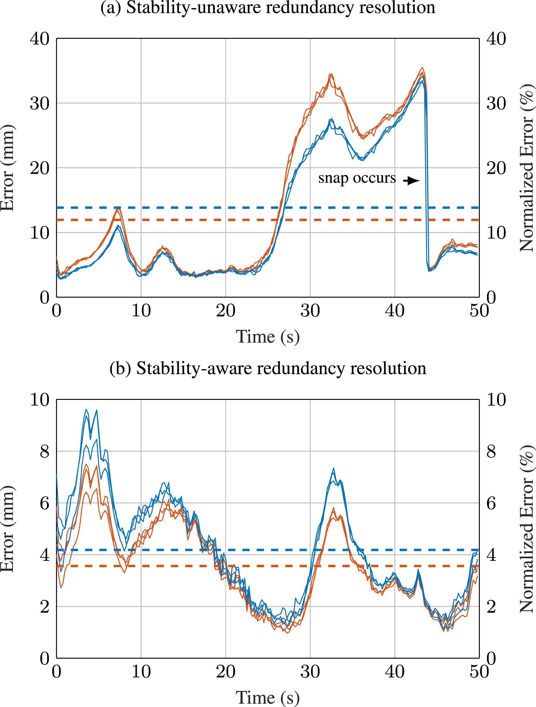

Note that these levels of error are excellent considering the intrinsic error in concentric tube robot models. The standard kinematic model for concentric tube robots does not include effects such as friction, tube clearances, and nonlinear material properties. Experimental evaluations of the model report errors of 1.5–3.0% (Rucker et al. 2010) and 2.1% (Dupont et al. 2010) of robot arclength. Thus, our results of 3.56±1.58% of arclength represent very good tracking.

It is interesting to note that a simulation of this experiment reveals that the stability measure goes below zero twice when not using instability avoidance, but only one snap occurred during the experimental trials. This is to be expected based on the experiments in (Gilbert et al. 2016b), which show the stability measure to be generally conservative, that is, the physical robot generally snaps at a relative angle greater than that predicted by the model due to unmodeled frictional effects.

4.1.2. Teleoperation experiment

Applying redundancy resolution methods to concentric tube robots to avoid elastic instabilities is motivated by the need for stable control without the significant computational overhead or a priori knowledge necessary for path planning. While the trajectory following experiment described above is not “pre-planned” (in the sense that the controller gets a new desired task space velocity at each time step and calculates a joint space velocity based only on that time step, without knowledge of the entire trajectory), it is still worthwhile to validate the algorithm’s performance in a teleoperated scenario with a user in the loop and no prescribed trajectory.

The user was instructed to control the tip position of the robot to explore the robot’s workspace. This was conducted with and without the instability avoidance control law. The user controlled the robot using a 3D Systems Touch haptic device. The user’s commanded tip position was compared to the previous position to compute the desired task space velocity ${\dot{\mathit{x}}}_{des}$ using (7).

Figure 13 shows all points that the robot can reach in stable configurations (blue) overlaid with all points that if reached would be unstable (red). Note that there is overlap between the two due to the robot’s redundancy—many points can be reached in both stable and unstable configurations. The user’s teleoperated position time history is overlaid using a black line. With instability avoidance turned off, the user experienced several uncontrolled snaps while moving the manipulator. These snapping points are marked with yellow diamonds in Figure 13. Results of this experiment can also be seen in Extension 2 (Table 5).

Figure 13.

Results of the teleoperation redundancy resolution experiment without instability avoidance (left) and with instability avoidance (right). In both cases, the tracked tip data is projected into the (R, z) plane describing the robot’s workspace, where 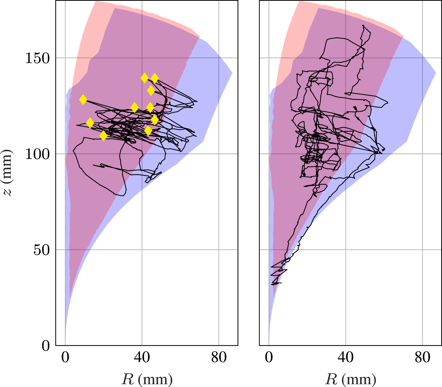$R=\sqrt{x^2+y^2}$ . The red region contains robot configurations that are unstable and physically unachievable, while the blue region contains configurations that are stable. The elastic stability-aware controller allowed the user to navigate the robot throughout the workspace without snapping. Without this control law, the robot snapped 10 times, as marked by the yellow diamonds.

This experiment demonstrates the importance of using the stability metric for redundancy resolution in a real-time control scenario on a prototype with highly curved tubes. Without the elastic stability-aware algorithm, the robot cannot be reliably teleoperated throughout much of its workspace.

4.2. Stiffness tuning experimental validation

To validate the stiffness tuning approach, we measured the tip deflection of a three-tube concentric tube robot. We used the stiffness tuning control law to first minimize and then maximize the maximum singular value of the compliance matrix σ _C while regulating the robot’s tip position, as described in the simulations of Section 3.2.

The same tube set was used for these experiments as were used in the instability avoidance experiments of Sec. 4.1. The commanded tip position was $\mathit{p}={\left[\mathrm{50,0,100}\right]}^{\mathsf{T}}$ mm. This is a suitable point for testing compliance, as the direction of σ _C in this configuration is approximately aligned with the y-axis of the robot base frame (i.e., vertically in the world frame).

To evaluate the tip stiffness of the robot, we hung a 50 g mass approximately 4 mm from the tip of the inner tube (shown in Figure 14). We measured the tip position with and without the applied load using the same electromagnetic tracking system as Section  4.1 in order to assess the position regulation error and the deflection. These measurements were taken at the nominal configuration (α _C = 0), the compliance minimization configuration (α _C = −300), and the compliance maximization configuration (α _C = 300). The robot was driven to these positions by commanding a constant tip position, changing the value of α _C , and waiting for the motors to stop moving (the ability of the robot to change compliance and maintain tip regulation is dictated by joint limits and the location of the desired position in the workspace). When no further changes in motor positions or σ _C were observed, tip position measurements were taken with and without the applied load. This procedure was repeated 5 times and the resulting mean and standard deviation for each configuration were computed.

Figure 14.

Experimental setup for the stiffness tuning redundancy resolution experiment. The robot maximized and minimized compliance while regulating tip position. A 50 g mass was hung from the tip of the robot and the resulting deflection was measured with the electromagnetic tracker.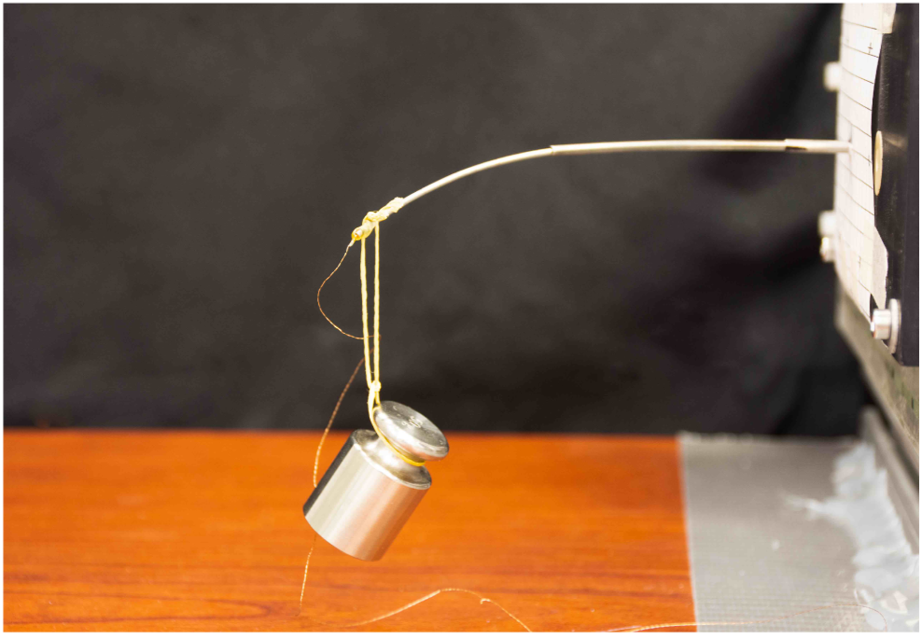

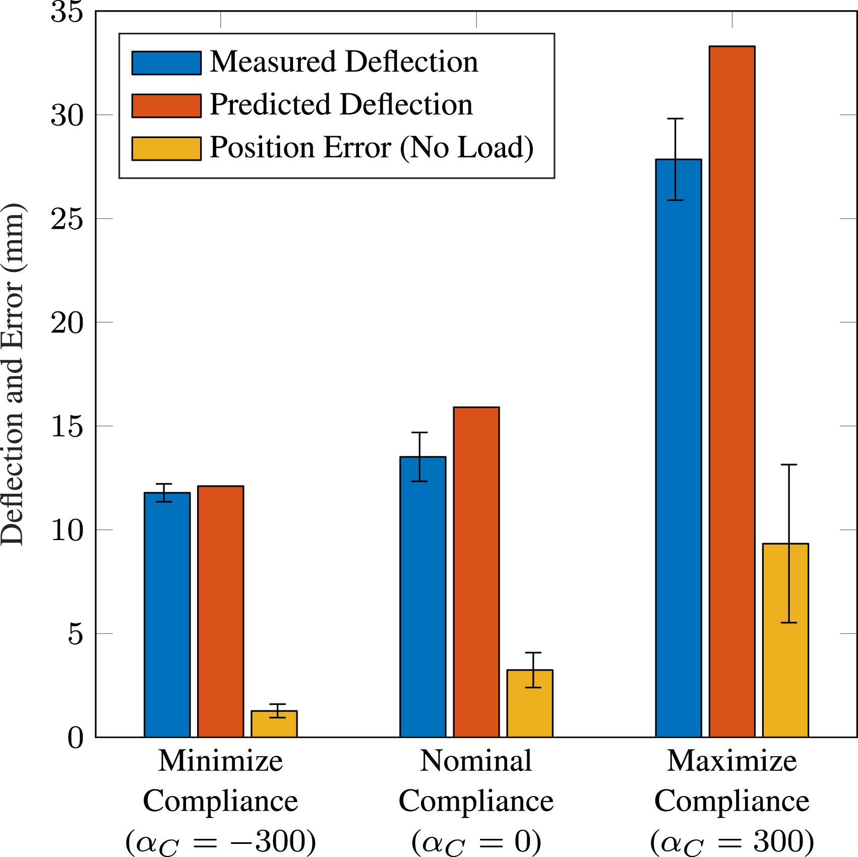
We compared our experimental results to a simulated robot, using the tip regulation simulation described in Section 3.2. The simulated robot achieved a nominal σ _C of 32.4 mm/N, minimized σ _C of 24.7 mm/N, and maximized σ _C of 67.8 mm/N. Using the nominal, minimized, and maximized σ _C , an applied load of 50 g produced predicted tip deflections of 15.9 mm, 12.1 mm, and 33.3 mm, respectively, in the robot’s most compliant direction. As shown in Figure 15, the corresponding measured deflections were 13.5±1.2 mm, 11.8±0.4 mm, and 27.8±2.0 mm. Figure 15 also shows the tip regulation error in all three cases, computed as the Euclidean norm between the commanded tip position p and the measured tip position with no load applied. The tip error was 3.23±0.84 mm in the nominal configuration, 1.27±0.32 mm in the minimized σ _C configuration, and 9.33±3.81 mm in the maximized σ _C configuration.

Figure 15.

Results of the robotic stiffness tuning experiment (N = 5 trials). When the compliance metric σ _C is minimized, the robot exhibits the least amount of tip deflection under an applied load; when σ _C is maximized, it exhibits the highest tip deflection. The measured tip deflections are all close in magnitude to the corresponding theoretical tip deflections in the robot’s most compliant direction. Also shown is the tip regulation error in the unloaded cases.

5. Discussion and conclusion

In this paper, we have proposed a redundancy resolution algorithm for concentric tube robots and shown that it can be implemented on robotic hardware. This approach can be employed using real-time resolved rates control, making it suitable for teleoperation, and utilizes new understanding of elastic stability. Use of this control approach makes it possible to use highly curved concentric tube robots that are capable of maneuvering in tight spaces, thus increasing the realistic design space of these robots.

We have also shown that concentric tube robots can resolve redundancy to tune their compliance. This ability could be used to improve the capabilities of these tools in the hands of surgeons and to allow the user to change the properties of their manipulator on the fly. We have demonstrated this capability with simulations and an example experimental configuration. Future work on redundancy resolution stiffness control of concentric tube robots includes further evaluation of the control scheme’s performance with different robot configurations. Different stiffness goals, such as optimizing axial or lateral stiffness, could be explored as well. In addition, it may be worthwhile to perform user studies in which the user can select the desired tip stiffness behavior. Improved designs and stiffness modification may one day combine to enable physicians to perform new kinds of surgical procedures that cannot be attempted today.

Supplemental Material

Supplemental Material