Stable nullspace adaptive parameter identification of 6 degree-of-freedom plant and actuator models for underactuated vehicles: Theory and experimental evaluation

Abstract

Model-based approaches to navigation, control, and fault detection that utilize precise nonlinear models of vehicle plant dynamics will enable more accurate control and navigation, assured autonomy, and more complex missions for such vehicles. This paper reports novel theoretical and experimental results addressing the problem of parameter estimation of plant and actuator models for underactuated underwater vehicles operating in 6 degrees-of-freedom (DOF) whose dynamics are modeled by finite-dimensional Newton-Euler equations. This paper reports the first theoretical approach and experimental validation to identify simultaneously plant-model parameters (parameters such as mass, added mass, hydrodynamic drag, and buoyancy) and control-actuator parameters (control-surface models and thruster models) in 6-DOF. Most previously reported studies on parameter identification assume that the control-actuator parameters are known a priori. Moreover, this paper reports the first proof of convergence of the parameter estimates to the true set of parameters for this class of vehicles under a persistence of excitation condition. The reported adaptive identification (AID) algorithm does not require instrumentation of 6-DOF vehicle acceleration, which is required by conventional approaches to parameter estimation such as least squares. Additionally, the reported AID algorithm is applicable under any arbitrary open-loop or closed-loop control law. We report simulation and experimental results for identifying the plant-model and control-actuator parameters for an L3 OceanServer Iver3 autonomous underwater vehicle. We believe this general approach to AID could be extended to apply to other classes of machines and other classes of marine, land, aerial, and space vehicles.

1. Introduction

This paper addresses the problem of simultaneously estimating the plant-model and control-actuator parameters for an underactuated underwater vehicle (UV) operating in 6 degrees-of-freedom (DOF). In particular, we report a new adaptive identification (AID) algorithm, including a novel proof of asymptotic parameter convergence, and associated simulation and experimental results.

To the best of our knowledge, this paper reports the first theoretical approach and experimental validation to identify simultaneously UV dynamical plant-model parameters (for critical terms such as mass, added mass, hydrodynamic drag, and buoyancy) and control-actuator parameters (for control-surface models and thruster models) in 6-DOF. Most previously reported studies on parameter identification assume that the control-actuator parameters are known a priori. Moreover, this paper reports the first proof of convergence of the parameter estimates to the true set of parameters for this class of vehicles when a persistence of excitation condition is satisfied. Most previously reported AID approaches for this class of systems only show stability and boundedness of the parameter estimates.

The performance of a dynamic model in predicting a robotic vehicle’s state depends primarily on the accuracy of the model structure and parameters. Accurate estimates of these parameters are required for model-based navigation, control, fault detection, and simulation. Indeed, a broad class of nonlinear model-based trajectory-tracking controllers for robot arms developed since the 1980s require exact knowledge of the plant’s kinematic and dynamic parameters—examples include nonlinear tracking controllers for second-order rotating plants Koditschek (1988) and exactly linearizing model-based trajectory-tracking controllers for open kinematic chains Freund (1983); Luh et al. (1980).

While the general form of dynamical plant models for underwater vehicles has been understood for decades, Society of Naval Architects and Marine Engineers (U.S.). Technical and Research Committee. Hydrodynamics Subcommittee (1950), the dynamic-model parameters—that is, parameters for terms including mass, added mass, hydrodynamic drag, buoyancy, and control actuators—are impossible to determine analytically and are often not provided by manufacturers of the robotic vehicles. In contrast to plant kinematic parameters, which are often easily obtained from design documents and generally do not vary with time, plant dynamic parameters generally must be measured empirically and may change over time. Sources of such changes may include but are not limited to: substantial payload changes to the vehicle or robotic arm; physical changes to the vehicle, such as lengthening or shortening a UV to accommodate different payloads; variation in ballasting and trim conditions; variation in water density which affects vehicle buoyancy; and changes to on-board equipment and instrumentation (both external and internal). Model parameters must be re-estimated whenever the robot physical configuration is significantly altered.

Estimating plant-model parameters is generally more difficult for underactuated, torpedo-shaped UVs than for fully actuated UVs with thrusters because: (i) the reduced actuation available on underactuated UVs limits the plant excitation that can be induced from the control inputs, and (ii) torpedo-shaped UVs and many uncrewed aerial vehicles (UAVs) are often actuated with control surfaces (e.g., fins, wings, elevators, and rudders), which are difficult to characterize independently of the plant-model parameters.

For these reasons, we seek an approach to parameter estimation for underactuated UVs in 6-DOF that simultaneously estimates plant and actuator parameters and can be performed routinely in the field with minimal time and effort by the vehicle operator. We believe the general approach to AID reported here is not limited to underwater vehicles and could be extended to apply to other classes of machines and other classes of marine, land, aerial, and space vehicles.

1.1. Motivation for accurate model identification

Model-based approaches to navigation, control, and fault detection that utilize precise nonlinear models of vehicle dynamics will enable more accurate control and navigation, assured autonomy, and more complex missions for robotic vehicles. In particular:

(1) Accurately identified model parameters can be utilized in forward simulation to predict vehicle performance and tune gains for various controllers (open-loop and closed-loop), navigation systems, and motion-planning algorithms.

(2) Accurately identified model parameters can be utilized in model-based state-estimation (navigation) systems that utilize the full UV plant model in their solution Harris and Whitcomb (2018).

(3) Accurately identified model parameters can enable model-based control algorithms that offer improved performance over traditional controllers. For example, previously reported studies have shown that nonlinear adaptive model-based control (AMBC) can outperform proportional derivative control (PDC) in trajectory tracking for fully actuated UVs McFarland and Whitcomb (2014) and fully actuated robot arms Craig et al. (1987); Slotine and Li (1987); Sadegh and Horowitz (1990); Whitcomb et al. (1993).

(4) Online approaches for identifying plant parameters may lead to new methods for online fault detection and fault-tolerant control of UVs, for example Mao and Whitcomb (2021).

1.2. Common approaches to parameter identification

The three most common approaches to model-parameter estimation for vehicles with dynamics that cannot be fully characterized analytically, such as UVs, are:

(1) utilizing data obtained in captive-motion experiments (e.g., towing a vehicle in a hydrodynamic test tank or wind tunnel),

(2) utilizing data from computational fluid dynamics (CFD) simulations, or

(3) utilizing data obtained in full-scale experimental trials of a robotic vehicle in controlled free motion (e.g., under open-loop or closed-loop control).

Captive-motion experiments are the standard in naval architecture Van Manen and Van Ossanen (1988); however, they are time consuming, expensive, and difficult to perform properly. Further, the results are valid only for the specific vehicle configuration tested, and it is often impractical to repeat the experiments for every possible configuration of the robotic vehicle. Typically, the experimental setup involves either rotating-arm experiments Van Manen and Van Ossanen (1988) or planar motion mechanism (PMM) experiments, such as towing a vehicle on a carriage with a load cell at a fixed velocity in a hydrodynamic test facility, for example, Prestero (2001). Captive-motion experiments can be quite accurate in certain DOF, but these experiments often require decoupling the DOF, which can lead to model inaccuracies. Typically, separate tests are conducted with and without the control surfaces (fins) installed in order to isolate the fin drag from the body drag, and separate test facilities are often required to characterize the fin lift and drag as a function of the angle of attack.

Parameter estimation based on computational fluid dynamics uses numerical models of fluid flow around the vehicle to simulate virtual PMM tests. CFD-based approaches to model identification vary widely in accuracy, time, and cost. Additionally, CFD-based approaches require detailed computer-aided design (CAD) models of the UV, which may be difficult or impossible to obtain from commerical off-the-shelf (COTS) UV manufacturers. If a CAD model is created by the end user for a COTS UV, often the vehicle is modeled as a smooth hull—appendages such as antennas, strobe lights, sensors (e.g., CTD sensors and sonar transducers), and acoustic modem transducers are left unmodeled Liu et al. (2020). An advantage of CFD-based parameter estimation, however, is the ability to inform design choices during the preliminary vehicle-design process Phillips et al. (2010).

While these approaches have advantages, both captive-motion experiments and CFD-based approaches are often infeasible for many UV end users for reasons of cost, time, and practicality.

Parameter identification based on data collected in full-scale experimental trials of UVs in controlled free motion has several advantages over captive-motion experiments and CFD. First, the approach is accessible to any end user who can deploy an existing UV. Additionally, though beyond the scope of this paper, some approaches that utilize full-scale experimental data, such as the approach described herein, can be extended to run in real time during vehicle missions. Such algorithms can also enable online model-based fault detection and fault isolation Mao and Whitcomb (2021).

1.3. Parameter identification of underactuated robotic vehicles

Many robots, such as torpedo-shaped autonomous underwater vehicles (AUVs), aerial drones, and aerospace vehicles are not fully actuated. Instead, these robots are underactuated. We adopt the following definition for Underactuated Control Differential Equations from Tedrake (2023): A second-order control differential equation described by the equations $\ddot{q}=f\left(q,\dot{q},u,t\right)$ is fully actuated in state $x={\left[q^T,{\dot{q}}^T\right]}^T$ and time t if the resulting map f is surjective: for every $\ddot{q}$ there exists a control input u such that $\ddot{q}=f\left(q,\dot{q},u,t\right)$ which produces the desired response. Otherwise it is underactuated (at state x at time t).

The robotic vehicle used to validate our theoretical results, an Iver3 (L3Harris OceanServer, Fall River, MA, USA) AUV, is clearly underactuated. The vehicle has only five control inputs (4 commanded fin angles and 1 commanded main propeller angular velocity), fewer than the UV’s 6-DOF. Thus, the Iver3 robotic vehicle is underactuated by definition, regardless of the particular method used to model the actuators. The Iver3 belongs to the common class of torpedo-shaped AUVs. This class of UV differs significantly from fully-thruster-actuated remotely operated vehicles (ROVs), where the thrusters are often capable of exerting arbitrary 6-DOF forces and moments on the vehicle. Torpedo-shaped UVs are controllable only when in forward motion, are generally incapable of hovering, and are physically unable to track fully general 6-DOF reference trajectories.

Parameter estimation of underactuated UVs presents real theoretical and practical challenges. A main concern is whether the UV parameters are observable. In other words: do the control actuators have sufficient control authority to excite the plant so that the plant model parameters are observable? The authors have previously defined necessary and sufficient conditions for mass and rotational-inertia parameters in rigid-body dynamical plants to be uniformly completely observable (UCO) Paine and Whitcomb (2021). Previously reported simulation studies confirmed that underactuated rigid-body plants can meet these conditions. We conjectured that a similar approach could be used to show UCO of other parameters such as drag coefficients and gravity terms. In this paper, via the equivalent concept of persistence of excitation (PE), we define sufficient conditions for convergence of plant and actuator parameter estimates to a true parameter set.

To the best of our knowledge, with the exception of Harris et al. (2018), Harris (2019), Paine (2018), upon which this work is based, there are no previously reported studies for parameter identification of underactuated robotic vehicles that simultaneously identify plant-model parameters and actuation parameters in 6-DOF.

With few exceptions, namely McFarland and Whitcomb (2021), many previously reported AID methods require model-based adaptive tracking controllers and are not applicable when the UV is operating under any control law other than a specific adaptive tracking controller. On commercially available robotic vehicles, including UVs, the user is often limited to using the proprietary control system provided by the manufacturer, and the user cannot easily replace the manufacturer’s proprietary controller with an adaptive trajectory-tracking controller (ATTC). The AID approach reported herein works for robotic plants operating under any control inputs (specifically, it not limited to the case of trajectory-tracking control), and is thus applicable in the common situation of a UV operating with a proprietary, manufacturer-provided controller or in open-loop control.

In summary, the advantages of this AID approach include:

• This AID method simultaneously estimates both plant and actuator parameters that are present in a physics-based model of robot dynamics, either fully actuated or underactuated. Most previously reported studies on parameter identification assume that the control-actuator parameters are known a priori.

• This AID method is the first reported AID approach with a proof of convergence of the parameter estimates to the true set of parameters for this class of vehicles, provided that a PE condition is satisfied. Most previously reported AID approaches for this class of systems only show stability and boundedness of the parameter estimates.

• This AID method, like other adaptive identifiers, does not require body-relative linear and angular acceleration signals, which is beneficial because body-relative linear acceleration terms are difficult to obtain. Although not discussed in detail here, we find this AID method is more robust to sensor noise when compared to the least-squares–based methods described in Harris et al. (2018).

• This AID method ensures stability and asymptotic convergence of the identification plant velocity error and convergence of the parameter estimates, in contrast to many machine learning (ML) approaches which are generally unable to provide such guarantees.

• The simulation and experimental studies reported here show that AID-estimated parameters can converge with a “single training set” containing on the order of 1000 seconds of free-motion AUV dive data, and the performance of the resulting model was verified in both self-validation and cross-validation.

• This AID method may be performed by a user in the field when the plant dynamics change, unlike captive-motion experiments or CFD.

• This AID method works with any open or closed-loop control law, provided that a PE condition is satisfied. Unlike many previously reported AID methods, this method does not require a trajectory-tracking controller, which is often unsuitable for underactuated vehicles without control authority in all DOF.

2. Literature review

Most previously reported model-based parameter identification methods employ one of two general approaches: (i) least-squares linear regression of experimental data or (ii) adaptive model-based trajectory-tracking control and adaptive identification. Khalil and Dombre provide a detailed overview of these approaches Khalil and Dombre (2002). We separately group machine learning (ML) and neural network (NN) techniques as a third type of method for system identification, because these methods do not explicitly use a dynamic model for all or part of the plant. Instead, these methods largely map plant input-to-output behavior. The following section describes recent work in these three areas and compares the different approaches.

2.1. Least squares and Kalman filtering

A variety of previously reported studies have employed least-squares, total least-squares, or extended Kalman filters to identify plant parameters entering linearly into the plant equations of motion for robot manipulators Khosla and Kanade (1985); Atkeson et al. (1986); An et al. (1988); Armstrong et al. (1986); Swevers et al. (2007), uncrewed underwater vehicles (UUVs) Caccia et al. (2000); Alessandri et al. (1998); Martin and Whitcomb (2014); Harris et al. (2018), and spacecraft Norman et al. (2011); Keim et al. (2006). Most methods require the time derivative of joint angles or time derivative of 6-DOF body-relative linear and angular velocity, which is difficult to measure directly, and often is numerically estimated by differentiating sensor measurements—a process that is sensitive to sensor noise. Some studies ameliorate the problem of sensor noise through use of signal filtering. However, unless performed using an acausal method, filtering introduces time delay. These issues are (sometimes) adequately handled during offline data processing, but pose a significant challenge for online parameter estimation.

2.2. Adaptive trajectory-tracking control

Adaptive model-based tracking controllers have been proposed for both fully actuated McFarland and Whitcomb (2014), Sahu and Subudhi (2014) and underactuated marine vehicles Jiang (2002), Aguiar and Hespanha (2007), spacecraft Ahmed et al. (1998), Wong et al. (2001), and mobile robots Fukao et al. (2000), Shojaei et al. (2011). However, precise definitions for persistence of excitation (PE) to ensure asymptotic convergence of parameter-estimation error are absent from many studies, such as Shojaei et al. (2011), Sahu and Subudhi (2014), Wong et al. (2001). PE-like conditions were reported in Aguiar and Hespanha (2007), with a focus on stability of the trajectory-tracking error and robustness to parametric uncertainty. Necessary and sufficient PE conditions for asymptotic identification were reported in Ahmed et al. (1998), but only for parameters in the inertia matrix for 3-DOF rotational plants.

In Craig et al. (1987) the authors report a stable adaptive trajectory-tracking algorithm for fully actuated robot arms that require instrumentation of joint acceleration. In Slotine and Li (1987); Sadegh and Horowitz (1990); Whitcomb et al. (1993) the authors report three different stable adaptive trajectory-tracking algorithms for fully actuated robot arms that do not require instrumentation of joint acceleration

2.2.1. Relationship of adaptive identification to adaptive trajectory tracking control

The present study addresses AID; it does not address the problem of simultaneously performing adaptive model identification and model-based trajectory tracking control, that is, ATTC. There are numerous previously reported results for ATTC of mechanical systems in which the plant state is controlled to follow a smooth trajectory known a priori. ATTC, however, will not work when either (i) the plant is underactuated or (ii) the plant is controlled by an existing controller that cannot be modified, as is often the case with commercially available robot systems, or (iii) the plant is under open-loop control, as is often the case for system identification experiments in the early stages of vehicle development.

In general, papers that report novel adaptive model-based tracking controllers prove convergence of the trajectory-tracking error, and prove stability and boundedness (but not convergence) of the parameter-estimation error.

2.3. Adaptive parameter estimation

Adaptive methods for parameter identification of linear time-invariant plants are well understood Narendra and Annaswamy (1989), Sastry and Bodson (1989), Astrom (1989), Tao (2003). In Hsu et al. (1987), the authors report an AID algorithm for robot arms that requires instrumentation of joint acceleration, as well as a low-pass filter approach for the parameter update law to avoid this requirement.

Relatively few studies have considered model-parameter identification of underactuated UVs, for example, Graver et al. (2003), or underactuated robot arms, for example, Ayusawa et al. (2014). To the best of our knowledge, only two previous studies, Paine and Whitcomb (2018), McFarland and Whitcomb (2021), have addressed AID of underactuated UVs.

Few UV parameter identification methods which do not require direct instrumentation of acceleration or trajectory-tracking controllers have been reported. The AID algorithm presented here may prove useful in applications with controlled or uncontrolled plants in which reference trajectory tracking is impractical or infeasible.

AIDs for fully actuated multi-DOF UV plant models were first reported by Smallwood and Whitcomb in Smallwood and Whitcomb (2003), but this AID was limited to fully diagonal plant models in which the dynamics of each DOF is fully decoupled and independent from the dynamics of other DOF. McFarland and Whitcomb in McFarland and Whitcomb (McFarland and Whitcomb, 2013, 2021) report an AID for fully coupled 6-DOF UV plant models; the AID algorithm applies to fully actuated or underactuated plants, and the experiments reported utilized 6-DOF actuation. That study is the foundation for the AID reported here. In Paine and Whitcomb (2018), Paine and Whitcomb reported an extension of the AID reported in McFarland and Whitcomb (2013) to 3-DOF underactuated UV plant models and includes a simulation study with Gaussian noise.

2.4. Machine learning

In their pioneering paper Narendra and Parthasarathy (1990), Narendra and Parthasarthy developed the theoretical foundations for the application of neural networks (NNs) to perform system identification of nonlinear dynamical plants. More recently, experimental results using ML and NN-based identification methods have been reported for underactuated UVs Wehbe et al. (2017), Wehbe and Krell (2017), Karras et al. (2013). Broad interest in using these methods for system identification has led to a variety of different approaches.

In general, ML approaches to model identification appear to be divided on the level to which they utilize physics-based models. Some authors caution against adopting techniques and algorithms from domains void of underlying physics (such as natural language processing) to the natural sciences; instead, these authors argue specifically for increased usage of physics-based models in ML Willcox et al. (2021). An interesting hybrid approach is reported in Woo et al. (2018), wherein the authors decompose the dynamics of a uncrewed surface vessel (USV) into linear and nonlinear terms; they estimate the parameters corresponding to the linear terms using the parameter-estimation technique from Sonnenburg and Woolsey (2013) and use ML for the nonlinear model. A similar hybrid approach for UVs was proposed in Van de Ven et al. (2007). In this case, the underlying structure of the nonlinear dynamic model is maintained via the careful design of separate neural networks to estimate each of the mass, damping, and buoyancy terms. However, other authors in ML, for example, Bagherzadeh (2018), argue against the use of a predetermined structure, saying that the use of predetermined model structure reduces the problem of model identification to one of parameter estimation, which may not fully capture the nonlinearities of the dynamics. Clearly, there is some disagreement in this field, and some researchers report satisfactory results obtained via their particular approach to system identification.

2.5. Approach comparison

We can offer some comparison of these approaches. Least-squares estimation is often performed offline with some signal filtering, whereas the adaptive techniques, including the AID reported herein, can be implemented online. Additionally, least-squares estimation typically requires signals of translational and rotational body-frame acceleration, while AIDs generally require only body-frame velocities. Although some argue that ML and NN methods may be able to perform system identification by capturing complex nonlinear dynamics that are difficult to model, these methods are not guaranteed to be stable or, in some cases, to generalize beyond the training data set. Additionally, in most cases, significant computational time and training data are needed to complete estimates using ML and NN methods. On the other hand, the adaptive techniques can be proven to be stable and to provide asymptotic error convergence, as we will show in Section 5.2 and 5.3.

3. Mathematical conventions

For a matrix $A\in {\mathbb{R}}^{n\times n}$ , we denote eigenvalues ordered from minimum to maximum magnitude as λ_min(A) ≤ λ_n−1(A)… ≤ λ₂(A) ≤ λ_max(A). For a vector $x\in {\mathbb{R}}^n$ , we define the following vector norm:

• Euclidean (L²) norm:

${\Vert x\Vert }_2={\left(x^{T}x\right)}^{1/2}$

(1)

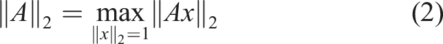
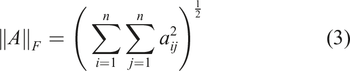
We also define the following norms on the matrix A:

• Spectral norm:

$\Vert A{\Vert }_2=\underset{{\Vert x\Vert }_2=1}{\max }\Vert Ax{\Vert }_2$

(2)

• Frobenius norm:

${\Vert A\Vert }_F={\left({\displaystyle \sum }_{i=1}^n{\displaystyle \sum }_{j=1}^n{a}_{ij}^2\right)}^{\frac{1}{2}}$

(3)

noting that ‖A‖₂ ≤ ‖A‖ _F . When not specified, the ‖ ·‖₂ norm is implied for both vectors and matrices.

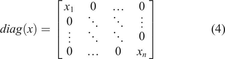
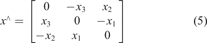
For a vector $x\in {\mathbb{R}}^n$ , we also define the functions:

• The diagonal matrix operator $\text{diag}(·):{\mathbb{R}}^n\to {\mathbb{R}}^{n\times n}$ such that $\forall x\in {\mathbb{R}}^n$ ,

$\mathit{diag}\left(x\right)=\left[\begin{array}{cccc}{x}_1& 0& \dots & 0\\ 0& \ddots & \ddots & ⋮\\ ⋮& \ddots & \ddots & 0\\ 0& \dots & 0& x_n\end{array}\right]$

(4)

• • The skew-symmetric operator ${(·)}^{\wedge }:{\mathbb{R}}^3\to {\mathbb{R}}^{3\times 3}$ such that $\forall x={\left[x_1\hspace{0.17em}{x}_2\hspace{0.17em}{x}_3\right]}^T\in {\mathbb{R}}^3$ ,

$x^{\wedge }=\left[\begin{array}{ccc}0& -x_3& x_2\\ x_3& 0& -x_1\\ -x_2& x_1& 0\end{array}\right]$

(5)

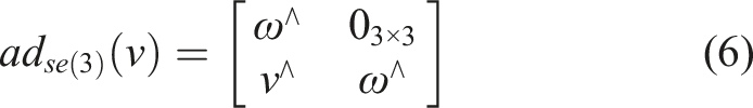
• The se(3) adjoint operator $ad(·):{\mathbb{R}}^6\to {\mathbb{R}}^{6\times 6}$ such that $\forall v={\left[{\nu }^T\hspace{0.17em}{\omega }^T\right]}^T\in {\mathbb{R}}^6$ ,

$a{d}_{se\left(3\right)}\left(v\right)=\left[\begin{array}{cc}{\omega }^{\wedge }& 0_{3\times 3}\\ {\nu }^{\wedge }& {\omega }^{\wedge }\end{array}\right]$

(6)

4. Finite-dimensional dynamical plant models for 6-DOF vehicles

We consider the class of plants which can be modeled by the Newton-Euler equations in body-relative coordinates. We assume the inertial terms include the mass of the body used in classical rigid-body dynamics, and also include the additional “added mass” or “hydrodynamic mass” arising from the accelerating/decelerating submerged body’s interaction with surrounding fluid. Furthermore, we consider that such plants can be subject to quadratic drag forces and net gravitational forces and moments.

4.1. State and control input representation

• $\eta \left(t\right)={\left[x{\left(t\right)}^T\hspace{0.17em}\phi {\left(t\right)}^T\right]}^T\in {\mathbb{R}}^6$ is the position and orientation of the body frame with respect to an inertial frame of reference, which contains the position of the body-frame origin $x\left(t\right)\in {\mathbb{R}}^3$ and its orientation in Euler angles $\phi \left(t\right)\in {\mathbb{R}}^3$ . We assume that roll and pitch are bounded to avoid the kinematic singularities arising in the Euler angle representation.

• $v\left(t\right)={\left[\nu {\left(t\right)}^T\hspace{0.17em}\omega {\left(t\right)}^T\right]}^T={\left[v_1\hspace{0.17em}{v}_2\hspace{0.17em}{v}_3\hspace{0.17em}{v}_4\hspace{0.17em}{v}_5\hspace{0.17em}{v}_6\right]}^T\in {\mathbb{R}}^6$ is the body-frame velocity, which contains the linear body velocity, $\nu \left(t\right)={\left[v_1\hspace{0.17em}{v}_2\hspace{0.17em}{v}_3\right]}^T\in {\mathbb{R}}^3$ , and angular body velocities, $\omega \left(t\right)={\left[v_4\hspace{0.17em}{v}_5\hspace{0.17em}{v}_6\right]}^T\in {\mathbb{R}}^3$ .

• $\dot{v}\left(t\right)={\left[{\dot{v}}_1\hspace{0.17em}{\dot{v}}_2\hspace{0.17em}{\dot{v}}_3\hspace{0.17em}{\dot{v}}_4\hspace{0.17em}{\dot{v}}_5\hspace{0.17em}{\dot{v}}_6\right]}^T\in {\mathbb{R}}^6$ is the time derivative of body-frame velocity.

• $\xi \left(t\right)\in {\mathbb{R}}^{k+i}$ is the control input vector, with k propellers and i hydrodynamic control surfaces (e.g., fins).

The control inputs ξ(t) for the specific vehicle studied in this paper are defined in Section 4.3 and Appendix A.

4.2. Commonly accepted plant model

This section describes the commonly accepted finite-dimensional nonlinear equations of motion for 6-DOF vehicles subject to quadratic drag and gravitational forces. We will provide a brief history of the development of this model for 6-DOF underwater vehicles. However, we argue that the nonlinear dynamics of many 6-DOF plants, including terrestrial, aerospace, and underwater vehicles, can be modeled by these same equations of motion, which are simply the Newton-Euler equations with additional terms to represent drag, buoyancy, and control forces.

4.2.1. History of the development of plant models for underwater vehicles

The dynamics of a rigid-body underwater vehicle includes the finite-dimensional dynamics of the rigid-body vehicle body itself and the infinite-dimensional dynamics of the fluid surrounding the vehicle. While the former can be described by a finite-dimensional ordinary differential equation (ODE), the latter is described by the incompressible Navier–Stokes equation. With the exception of a few special cases, the infinite-dimensional Navier–Stokes equation has no closed-form solution and, for the case of marine vehicles, generally cannot be solved in real time (Larsson et al. 1998).

The most commonly accepted finite-dimensional models for submarine vehicles trace their lineage to studies beginning in the late 1950s and early 1960s at the U.S. Navy’s David Taylor Model Basin, (Goodman, 1960, Imlay, 1961), which referred to mass of the system resulting from immersion in a fluid as “added mass” and “derivative mass.” In Gertler and Hagen (1967), Feldman (1979) the authors expanded upon these equations, which have since become widely known as the “Standard equations of motion for submarine simulation” (Gertler and Hagen, 1967) and the “DTNSDC revised standard submarine equations of motion” (Feldman, 1979). More recently, Fossen in Fossen (1994, 2002) built upon these earlier studies to express in matrix form the equations of motion of an immersed body subject to non-conservative hydrodynamic forces. The matrix model is now commonly used throughout the literature.

4.2.2 Plant model

The commonly accepted second-order finite-dimensional dynamic model of this class of dynamical plants, as described in a body-relative frame coincident with the center of mass, is given by

$\tau \left(v,\phi ,\xi \right)=M\dot{v}+C\left(v\right)v+D_q\left(v\right)v+\mathcal{G}\left(\phi \right)$

(7)

where

• • $\tau \left(v,\phi ,\xi \right)\in {\mathbb{R}}^6$ is the vector of control-actuator forces and moments acting on the rigid body,

• • $M\in {\mathbb{R}}^{6\times 6}$ is the diagonal positive definite symmetric (PDS) inertia matrix,

• • $C\left(v\right)\in {\mathbb{R}}^{6\times 6}$ is the Coriolis matrix,

• • $D_q\left(v\right)\in {\mathbb{R}}^{6\times 6}$ is the quadratic hydrodynamic drag matrix, and

• • $\mathcal{G}\left(\phi \right)\in {\mathbb{R}}^6$ is the vector of buoyancy or gravitational forces and moments.

The body-frame angular velocity vector $v\left(t\right)\in {\mathbb{R}}^6$ and the time derivative of the body-frame position and attitude vector $\dot{\eta }\left(t\right)\in {\mathbb{R}}^6$ are related by the kinematic equation

$\dot{\eta }\left(t\right)=J\left(\eta \left(t\right)\right)v\left(t\right)$

(8)

where $J\left(\eta \right)\in {\mathbb{R}}^{6\times 6}$ is the usual kinematic Jacobian relation between v(t) and $\dot{\eta }\left(t\right)$ , which remains bounded for bounded pitch, as described in Section 2.2.1 of Fossen (1994).

Rearranging (7) to find the time derivative of the body velocity, $\dot{v}\left(t\right)$ , yields

$\dot{v}=M^{-1}(-C\left(v\right)v-D_q\left(v\right)v-\mathcal{G}\left(\phi \right)+\tau \left(v,\phi ,\xi \right)).$

(9)

In the sequel, for convenience we will use the term “plant acceleration” to denote $\dot{v}\left(t\right)$ , the time derivative of the body velocity defined in (9).

We assume the mass matrix is diagonal and can have different inertia quantities in each translational degree of freedom, that is, each diagonal entry of M can be unique. This is a common way to model hydrodynamic “added mass,” that is

$M=\text{diag}\left({\left[m_{11}\hspace{0.17em}{m}_{22}\hspace{0.17em}{m}_{33}\hspace{0.17em}{m}_{44}\hspace{0.17em}{m}_{55}\hspace{0.17em}{m}_{66}\right]}^T\right)$

(10)

$=\text{diag}\left({\theta }_m\right)$

(11)

where ${\theta }_m\triangleq {\left[m_{11}\hspace{0.17em}{m}_{22}\hspace{0.17em}{m}_{33}\hspace{0.17em}{m}_{44}\hspace{0.17em}{m}_{55}\hspace{0.17em}{m}_{66}\right]}^T\in {\mathbb{R}}^6$ is the mass parameter vector. Because the mass parameters enter linearly into the vector-valued function $M\dot{v}\in {\mathbb{R}}^6$ , we can factor $M\dot{v}$ such that

$M\dot{v}=W_m\left(\dot{v}\right){\theta }_m,$

(12)

where $W_m\left(\dot{v}\right)\in {\mathbb{R}}^{6\times 6}$ is the mass regressor matrix-valued function.

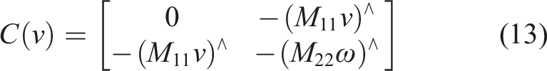
We parameterize the Coriolis matrix C(v) from M,

$C\left(v\right)=\left[\begin{array}{cc}0& -{\left(M_{11}\nu \right)}^{\wedge }\\ -{\left(M_{11}\nu \right)}^{\wedge }& -{\left(M_{22}\omega \right)}^{\wedge }\end{array}\right]$

(13)

where (·)^∧ is the skew-symmetric operator defined in (5), $M_{11}\triangleq \text{diag}\left({\left[m_{11}\hspace{0.17em}{m}_{22}\hspace{0.17em}{m}_{33}\right]}^T\right)$ and $M_{22}\triangleq \text{diag}\left({\left[m_{44}\hspace{0.17em}{m}_{55}\hspace{0.17em}{m}_{66}\right]}^T\right)$ . Equivalently, we can write

$C\left(v\right)v=a{d}_{se\left(3\right)}\left(v\right)Mv$

(14)

and because the mass parameters enter linearly into (14), we have the factorization

$C\left(v\right)v=a{d}_{se\left(3\right)}\left(v\right)W_m\left(v\right){\theta }_m$

(15)

where $W_m\left(v\right)\in {\mathbb{R}}^{6\times 6}$ is the same mass regressor matrix as in (12), with the velocity v instead of the plant acceleration $\dot{v}$ as its argument, and θ _m is the same mass parameter vector.

We assume the quadratic drag matrix, D _q (v), is diagonal positive semidefinite such that

$D_q\left(v\right)=\text{diag}\left(\left|v\right|\right)\hspace{0.17em}\text{diag}\left({\left[d_{11}\hspace{0.17em}{d}_{22}\hspace{0.17em}{d}_{33}\hspace{0.17em}{d}_{44}\hspace{0.17em}{d}_{55}\hspace{0.17em}{d}_{66}\right]}^T\right)$

(16)

$=\text{diag}\left(\left|v\right|\right)\text{diag}\left({\theta }_d\right)$

(17)

with ${\theta }_d\triangleq {\left[d_{11}\hspace{0.17em}{d}_{22}\hspace{0.17em}{d}_{33}\hspace{0.17em}{d}_{44}\hspace{0.17em}{d}_{55}\hspace{0.17em}{d}_{66}\right]}^T\in {\mathbb{R}}^6$ containing all of the drag parameters. We can again factor the linearly-entering parameters from (17), yielding

$D_q\left(v\right)v=\text{diag}\left(\left|v\right|\right)\text{diag}\left({\theta }_d\right)v$

(18)

$=\text{diag}\left(\left|v\right|\right)\text{diag}\left(v\right){\theta }_d$

(19)

$=W_d\left(v\right){\theta }_d$

(20)

where $W_d\left(v\right)\in {\mathbb{R}}^{6\times 6}$ is the drag regressor matrix-valued function.

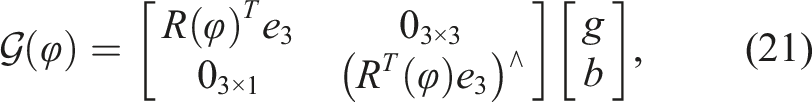
We define the function $\mathcal{G}\left(\phi \right)\in {\mathbb{R}}^{6\times 1}$ , which represents the gravitational forces and moments arising from net effective mass and righting moments,

$\mathcal{G}\left(\phi \right)=\left[\begin{array}{cc}R{\left(\phi \right)}^T{e}_3& 0_{3\times 3}\\ 0_{3\times 1}& {\left(R^T\left(\phi \right)e_3\right)}^{\wedge }\end{array}\right]\left[\begin{array}{c}g\\ b\end{array}\right],$

(21)

where $e_3={\left[\begin{array}{ccc}0& 0& 1\end{array}\right]}^T$ , $g=g_c\left(m-\rho \nabla \right)\in \mathbb{R}$ is the net effective buoyant force (in Newtons) with gravitational acceleration constant g _c , dry mass m, and displacement volume ∇, which displaces fluid with density ρ. The vector $b=g_c\overline{b}\rho \nabla \in {\mathbb{R}}^3$ represents the net righting torque (in Newton-meters) resulting from a center of buoyancy not co-incident with the center of mass, where $\overline{b}\in {\mathbb{R}}^3$ is the vector from the center of mass to the center of buoyancy. We note that this formulation assumes the origin of the body frame is at the center of mass of the UV. Factoring the linearly-entering parameters from (21), we have

$\mathcal{G}\left(\phi \right)=W_{\mathcal{G}}\left(\phi \right){\theta }_{\mathcal{G}},$

(22)

where $W_{\mathcal{G}}\left(\phi \right)\in {\mathbb{R}}^{6\times 4}$ is the gravitational regressor matrix-valued function and ${\theta }_{\mathcal{G}}={\left[\begin{array}{cc}g& b^T\end{array}\right]}^T\in {\mathbb{R}}^4$ is the gravitational parameter vector, which is composed of both the buoyancy and righting-moment parameters.

4.2.3 Actuator model

The vector $\tau \left(v,\phi ,\xi \right)\in {\mathbb{R}}^6$ represents the model of control-actuator forces and moments that are a result of body velocity v, attitude of the vehicle φ, and the control inputs $\xi \in {\mathbb{R}}^{k+i}$ to the control actuators, such as fin angle and propeller angular velocity, with parameters ${\theta }_a\in {\mathbb{R}}^a$ . If the actuation parameters θ _a enter linearly into τ(v, φ, ξ), as is true for the UV actuator model described explicitly in Appendix A, then we may factor the control vector such that

$\tau \left(v,\phi ,\xi \right)=W_a\left(v,\phi ,\xi \right){\theta }_a,$

(23)

where $W_a\left(v,\phi ,\xi \right)\in {\mathbb{R}}^{6\times a}$ is the (usually) nonlinear actuator regressor matrix and ${\theta }_a\in {\mathbb{R}}^a$ is the parameter vector that contains the minimum number of parameters required to fully characterize the control actuators.

The AID in this study is applicable to actuator models of the general form (23), with linearly-entering parameters and the additional requirement that W _a (v, φ, ξ) be uniformly continuous in v, φ, ξ and bounded for bounded v, φ, ξ.

4.3. Combined parameter vector

4.3.1. Plant parameters

In summary, our goal is to identify the following plant parameters:

• Mass parameters:

${\theta }_m={\left[m_{11}\hspace{1em}{m}_{22}\hspace{1em}{m}_{33}\hspace{1em}{m}_{44}\hspace{1em}{m}_{55}\hspace{1em}{m}_{66}\right]}^T\in {\mathbb{R}}^6$

(24)

• • Drag parameters:

${\theta }_d={\left[d_{11}\hspace{1em}{d}_{22}\hspace{1em}{d}_{33}\hspace{1em}{d}_{44}\hspace{1em}{d}_{55}\hspace{1em}{d}_{66}\right]}^T\in {\mathbb{R}}^6$

(25)

• • Buoyant-force and righting moment parameters:

${\theta }_{\mathcal{G}}={\left[g\hspace{1em}{b}_1\hspace{1em}{b}_2\hspace{1em}{b}_3\right]}^T\in {\mathbb{R}}^4$

(26)

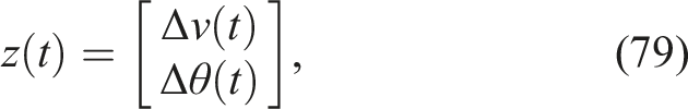
For convenience, we define the combined plant parameter vector

${\theta }_p\triangleq {\left[\begin{array}{ccc}{\theta }_m^T& {\theta }_d^T& {\theta }_{\mathcal{G}}^T\end{array}\right]}^T\in {\mathbb{R}}^p.$

(27)

4.3.2. Control-actuator parameters

Our goal is to identify the following fin and thruster actuator parameters, described in greater detail in Appendix A. For convenience, we define the control-actuator parameter vector

${\theta }_a\triangleq {\left[\begin{array}{ccc}{\theta }_{a_1}& \dots & {\theta }_{a_a}\end{array}\right]}^T\in {\mathbb{R}}^a.$

(28)

4.3.3. Plant and actuator parameter vector

We define the full plant and actuator parameter vector as

$\theta \triangleq {\left[\begin{array}{cc}{\theta }_p^T& {\theta }_a^T\end{array}\right]}^T\in {\mathbb{R}}^{\left(p+a\right)}.$

(29)

For our specific parameterization of the Iver3 AUV used for experimental validation, the dimensionality of θ is ${\mathbb{R}}^{\left(p+a\right)}={\mathbb{R}}^{\left(16+6\right)}={\mathbb{R}}^{22}$ . The details regarding the a = 6 actuator parameters for the Iver3 AUV are described in Appendix A. However, in the sequel we continue to use $\theta \in {\mathbb{R}}^{\left(p+a\right)}$ where possible for generality.

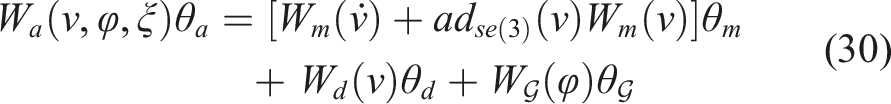
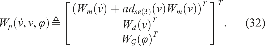
4.4. Regressor formulation of plant and actuator dynamics

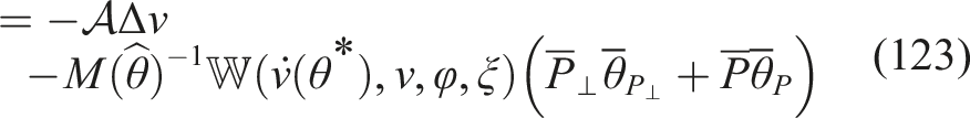
The equations of motion (7) can be written in regressor form by utilizing (12), (15), (20), (22), and (23), which yields

$\begin{array}{l}{W}_a\left(v,\phi ,\xi \right){\theta }_a=\left[W_m\left(\dot{v}\right)+a{d}_{se\left(3\right)}\left(v\right)W_m\left(v\right)\right]{\theta }_m\\ +W_d\left(v\right){\theta }_d+W_{\mathcal{G}}\left(\phi \right){\theta }_{\mathcal{G}}\end{array}$

(30)

$\begin{array}{c}{W}_a\left(v,\phi ,\xi \right){\theta }_a=W_p\left(\dot{v},v,\phi \right){\theta }_p\end{array}$

(31)

where the plant regressor $W_p\left(\dot{v},v,\phi \right)\in {\mathbb{R}}^{6\times p}$ is defined as

$W_p\left(\dot{v},v,\phi \right)\triangleq {\left[\begin{array}{c}{\left(W_m\left(\dot{v}\right)+a{d}_{se\left(3\right)}\left(v\right)W_m\left(v\right)\right)}^T\\ W_d{\left(v\right)}^T\\ W_{\mathcal{G}}{\left(\phi \right)}^T\end{array}\right]}^T.$

(32)

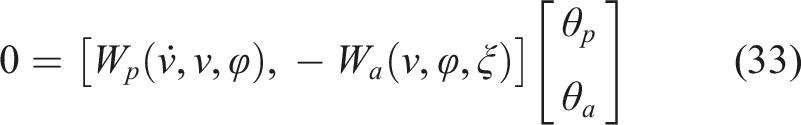
Rearranging (31) to combine the plant and control-actuator dynamics yields

$\begin{array}{c}0=\left[W_p\left(\dot{v},v,\phi \right),-W_a\left(v,\phi ,\xi \right)\right]\left[\begin{array}{c}{\theta }_p\\ {\theta }_a\end{array}\right]\end{array}$

(33)

$=\mathbb{W}\left(\dot{v},v,\phi ,\xi \right)\theta$

(34)

where $\mathbb{W}\left(\dot{v},v,\phi ,\xi \right)\in {\mathbb{R}}^{6\times \left(p+a\right)}$ is the (known) time-varying combined plant-and-actuator regressor matrix-valued function, defined as

$\begin{array}{c}\mathbb{W}\left(\dot{v},v,\phi ,\xi \right)\triangleq \left[W_p\left(\dot{v},v,\phi \right),-W_a\left(v,\phi ,\xi \right)\right]\end{array}$

(35)

$={\left[\begin{array}{c}{\left(W_m\left(\dot{v}\right)+a{d}_{se\left(3\right)}\left(v\right)W_m\left(v\right)\right)}^T\\ W_d{\left(v\right)}^T\\ W_{\mathcal{G}}{\left(\phi \right)}^T\\ -W_a{\left(v,\phi ,\xi \right)}^T\end{array}\right]}^T.$

(36)

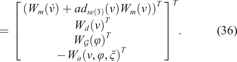
4.5. Regressor nullspace properties

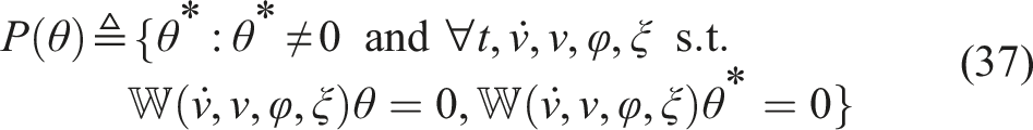
4.5.1. Non-uniqueness of the parameter vector

To the best of our knowledge, previous studies of UV model identification, with the exception of Harris et al. (2018) and Paine (2018), assume that the actuator parameters are known. When the actuator parameters are known and the plant model is minimally parameterized, the true plant parameters represent a single, unique point in the linear vector space of possible plant parameters.

In contrast, the AID addressed herein identifies plant and actuator parameters simultaneously. From (34), we note that $\theta \in {\mathbb{R}}^{\left(p+a\right)}$ is in the nullspace of the combined regressor $\mathbb{W}\left(\dot{v},v,\phi ,\xi \right)$ for an evolution of $\dot{v}\left(t\right),v\left(t\right),\phi \left(t\right),\xi \left(t\right)$ that satisfies the plant equation of motion (7).

A consequence of this nullspace structure is that many different parameter vectors satisfy the same equations of motion, even when the model is minimally parameterized. As an example, any nonzero scalar multiple of θ equivalently satisfies (34) and thus also satisfies (7).

Given a “true” parameter vector $\theta \in {\mathbb{R}}^{p+a}$ and all possible bounded evolutions of $\dot{v},v,\phi ,\xi$ that satisfy the plant equation of motion (7), and thus also satisfy the nullspace relationship (34) for this θ, there is then also a set $P\left(\theta \right)\subset {\mathbb{R}}^{\left(p+a\right)}$ of all nonzero parameter vectors θ* that equivalently satisfy (7) for the same evolutions of $\dot{v},v,\phi ,\xi$ and (34) for the regressor matrix-valued function $\mathbb{W}\left(\dot{v},v,\phi ,\xi \right)$ of these arguments. This set P(θ) is the “persistent nullspace” of the regressor, defined as

$\begin{array}{l}P\left(\theta \right)\triangleq \{{\theta }^{*}:{\theta }^{*}\ne 0\text{and}\forall t,\dot{v},v,\phi ,\xi \mathrm{s}.\mathrm{t}.\\ \mathbb{W}\left(\dot{v},v,\phi ,\xi \right)\theta =0,\mathbb{W}\left(\dot{v},v,\phi ,\xi \right){\theta }^{*}=0\}\end{array}$

(37)

Thus, the “true” parameter vector is not only a unique single vector in the parameter space ${\mathbb{R}}^{p+a}$ , but any element of the set P(θ). Note that the set P(θ) does not contain the origin, and that the set P(θ) ∪ 0 is a linear vector subspace of ${\mathbb{R}}^{\left(p+a\right)}$ .

In Section 4.5.2, we explore the identical input-output plant dynamics that arise from different parameter vectors in P(θ). These properties will be utilized in Section 5, where we report a novel adaptive identifier for θ and show that under a persistence of excitation (PE) condition, the estimate of θ converges to the true parameter set P(θ).

4.5.2. Acceleration input-output dynamics

We now prove our earlier claim that the input-output dynamics of (7), namely the resulting plant acceleration given control inputs and parameters, are the same for any parameter vector belonging to the true parameter set P(θ).

From the plant acceleration (9), after making the appropriate regressor substitutions (15), (20), and (22), as well as writing the true mass M as a function of the parameter vector θ ∈ P(θ) from which it arises, we obtain

$\begin{array}{l}\dot{v}=M{\left(\theta \right)}^{-1}(-a{d}_{se\left(3\right)}\left(v\right)W_m\left(v\right){\theta }_m-W_d\left(v\right){\theta }_d\\ -W_{\mathcal{G}}\left(\phi \right){\theta }_{\mathcal{G}}+W_a\left(v,\phi ,\xi \right){\theta }_a).\end{array}$

(38)

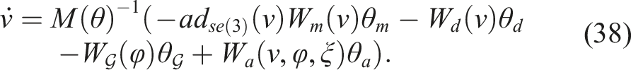
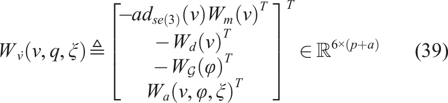
Observing the structure of (38), we define $W_{\dot{v}}\left(v,\phi ,\xi \right)\in {\mathbb{R}}^{6\times \left(p+a\right)}$ as

$W_{\dot{v}}\left(v,q,\xi \right)\triangleq {\left[\begin{array}{c}-a{d}_{se\left(3\right)}\left(v\right)W_m{\left(v\right)}^T\\ -W_d{\left(v\right)}^T\\ -W_{\mathcal{G}}{\left(\phi \right)}^T\\ W_a{\left(v,\phi ,\xi \right)}^T\end{array}\right]}^T\in {\mathbb{R}}^{6\times \left(p+a\right)}$

(39)

$=\left[W_m\left(\dot{v}\right)\hspace{0.17em}{0}_{6\times \left(p+a-6\right)}\right]-\mathbb{W}\left(\dot{v},v,\phi ,\xi \right),$

(40)

which allows us to write the plant acceleration $\dot{v}$ (38) as a function of the underlying parameters θ:

$\dot{v}=\dot{v}\left(\theta \right)\triangleq M{\left(\theta \right)}^{-1}{W}_{\dot{v}}\left(v,\phi ,\xi \right)\theta .$

(41)

Now we choose another vector θ* ∈ P(θ). By definition of P(θ) (37), we have the nullspace equation

$\mathbb{W}\left(\dot{v},v,\phi ,\xi \right){\theta }^{*}=0,$

(42)

which, substituting (40), results in

$\begin{array}{c}\left(\left[W_m\left(\dot{v}\right),0_{n\times \left(p+a-6\right)}\right]-W_{\dot{v}}\left(v,\phi ,\xi \right)\right){\theta }^{*}=0\end{array}$

(43)

$\begin{array}{c}M\left({\theta }^{*}\right)\dot{v}-W_{\dot{v}}\left(v,\phi ,\xi \right){\theta }^{*}=0\end{array}$

(44)

With further rearranging, we have

$\begin{array}{c}M\left({\theta }^{*}\right)\dot{v}=W_{\dot{v}}\left(v,\phi ,\xi \right){\theta }^{*}\end{array}$

(45)

$\begin{array}{c}\dot{v}=M{\left({\theta }^{*}\right)}^{-1}{W}_{\dot{v}}\left(v,\phi ,\xi \right){\theta }^{*}\end{array}$

(46)

and thus obtain an equivalent expression to (9) for the plant acceleration $\dot{v}$ , where (46) can also be written as a function of its parameter vector

$\begin{array}{c}\dot{v}\left({\theta }^{*}\right)\triangleq M{\left({\theta }^{*}\right)}^{-1}{W}_{\dot{v}}\left(v,\phi ,\xi \right){\theta }^{*}\end{array}$

(47)

$=\dot{v}$

(48)

$=\dot{v}\left(\theta \right)$

(49)

which verifies our claim in Section 4.5.1 that any parameter vector θ ∈ P(θ) yields the same input–output behavior.

It is important to note that a nonzero parameter vector $\stackrel{\sim }{\theta }\notin P\left(\theta \right)$ by definition does not satisfy $\mathbb{W}\left(\dot{v}\left(\theta \right),v,\phi ,\xi \right)\stackrel{\sim }{\theta }=0\forall t$ and over all $\dot{v}\left(\theta \right),v,\phi ,\xi$ that satisfy (7, 34) for the underlying true parameter vector θ. However, given $\stackrel{\sim }{\theta }\notin P\left(\theta \right)$ we can define a corresponding acceleration signal arising from these parameters

$\dot{v}\left(\stackrel{\sim }{\theta }\right)\triangleq M{\left(\stackrel{\sim }{\theta }\right)}^{-1}{W}_{\dot{v}}\left(v,\phi ,\xi \right)\stackrel{\sim }{\theta }.$

(50)

The term $\dot{v}\left(\stackrel{\sim }{\theta }\right)$ , (50), represents the time derivative of the body velocity given the same velocity v, attitude φ, and control inputs ξ as before, but for the different set of parameters $\stackrel{\sim }{\theta }$ .

We can obtain an analogous nullspace relationship to (34) for $\dot{v}\left(\stackrel{\sim }{\theta }\right)$ by rearranging (50) and substituting the regressor form of the inertia term defined in (12), which yields

$\begin{array}{c}M\left(\stackrel{\sim }{\theta }\right)\dot{v}\left(\stackrel{\sim }{\theta }\right)=W_{\dot{v}}\left(v,\phi ,\xi \right)\stackrel{\sim }{\theta }\end{array}$

(51)

$\begin{array}{c}{W}_m\left(\dot{v}\left(\stackrel{\sim }{\theta }\right)\right){\stackrel{\sim }{\theta }}_m=W_{\dot{v}}\left(v,\phi ,\xi \right)\stackrel{\sim }{\theta },\end{array}$

(52)

and applying (40), we obtain

$\begin{array}{c}{W}_m\left(\dot{v}\left(\stackrel{\sim }{\theta }\right)\right){\stackrel{\sim }{\theta }}_m-W_{\dot{v}}\left(v,\phi ,\xi \right)\stackrel{\sim }{\theta }=0\end{array}$

(53)

$\begin{array}{c}\left[\left[W_m\left(\dot{v}\left(\stackrel{\sim }{\theta }\right)\right)\hspace{0.17em}{0}_{6\times \left(p+a-6\right)}\right]-W_{\dot{v}}\left(v,\phi ,\xi \right)\right]\stackrel{\sim }{\theta }=0\end{array}$

(54)

$\begin{array}{c}\mathbb{W}\left(\dot{v}\left(\stackrel{\sim }{\theta }\right),v,\phi ,\xi \right)\stackrel{\sim }{\theta }=0.\end{array}$

(55)

In other words, when the plant acceleration in the regressor matrix (34) is replaced by an acceleration resulting from a different parameter class, $\dot{v}\left(\stackrel{\sim }{\theta }\right)$ , we have an analogous nullspace relationship $\stackrel{\sim }{\theta }\in \text{null}\left(\mathbb{W}\left(\dot{v}\left(\stackrel{\sim }{\theta }\right),v,\phi ,\xi \right)\right)$ , which holds ∀t and over all $\dot{v}\left(\stackrel{\sim }{\theta }\right),v,\phi ,\xi$ that satisfy (7,34) given a different parameter class $P\left(\stackrel{\sim }{\theta }\right)$ . We utilize this fact in the design of the adaptive identifier reported in Section 5.

5. Adaptive identifier

This section reports the theoretical derivation and stability analysis of a new adaptive identification (AID) algorithm for plants of the form (7). The AID reported herein significantly expands upon and extends a previous approach for adaptive parameter estimation of UV plant models by McFarland and Whitcomb (McFarland and Whitcomb, 2013, 2021). The specific differences are:

(1) The AID reported herein performs simultaneous identification of plant and actuator model parameters. In contrast, the AID reported in McFarland and Whitcomb (McFarland and Whitcomb, 2013, 2021) identifies only plant parameters.

(2) This study provides a mathematical proof of stability and of parameter-estimate convergence. In contrast, McFarland and Whitcomb (McFarland and Whitcomb, 2013, 2021) provide only a stability proof.

Problem Statement: The goal of this adaptive identification algorithm is to estimate the parameters θ (29) for plants and actuators of the form (7) or, equivalently, of the form (34), using only the available signals of vehicle attitude φ(t), linear and angular body velocity v(t), and the control input ξ(t).

Error Coordinates: We define the velocity error $\mathrm{\Delta }v\left(t\right)\in {\mathbb{R}}^6$ as the difference between the velocity $\widehat{v}\left(t\right)\in {\mathbb{R}}^6$ of an identification plant, whose dynamics are defined in (63), and the actual vehicle velocity, $v\left(t\right)\in {\mathbb{R}}^6$ , whose dynamics are defined in (9) (and equivalently in (41)), as

$\mathrm{\Delta }v\left(t\right)\triangleq \widehat{v}\left(t\right)-v\left(t\right).$

(56)

We define the vector of parameter estimates as $\widehat{\theta }\left(t\right)\in {\mathbb{R}}^{p+a}$ and choose a constant parameter vector ${\theta }^{*}\in {\mathbb{R}}^{p+a}$ , θ* ∈ P(θ), from the set P(θ) of “true” parameters defined in (37), which results in the error coordinates

$\mathrm{\Delta }\theta \left(t\right)\triangleq \widehat{\theta }\left(t\right)-{\theta }^{*}.$

(57)

Task: Our task is to design update laws $\dot{\widehat{v}}$ , $\stackrel{.}{\widehat{\theta }}$ for the identification plant and estimated parameters, respectively, such that all signals remain bounded and

$\underset{t\to \infty }{\lim }\mathrm{\Delta }v\left(t\right)=0,$

(58)

$\underset{t\to \infty }{\lim }\widehat{\theta }\in P\left(\theta \right).$

(59)

Assumptions: We make the following assumptions.

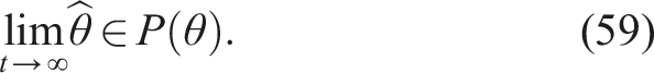
• v(t), η(t), ξ(t) are bounded.

• $\mathbb{W}\left(\dot{v}\left({\theta }^{*}\right),v,\phi ,\xi \right)$ (35) is locally uniformly continuous in $\dot{v}\left({\theta }^{*}\right),v,\phi ,\xi$ and a bounded function of these variables.

• As a result, $W_{\dot{v}}\left(v,\phi ,\xi \right)$ (39) is locally uniformly continuous in v, φ, ξ and a bounded function of these variables.

• The control inputs ξ are uniformly continuous in time and bounded.

• The true parameters θ* are bounded and constant.

• $\widehat{v}\left(t_0\right)=v\left(t_0\right)$ , that is Δv(t₀) = 0

• $\exists ϵ\in {\mathbb{R}}^{+}$ such that $\mathcal{T}{\left(t_0\right)}^{1/2}+ϵ\le {\lambda }_{\min }\left(M\left({\theta }^{*}\right)\right)$ , where

$\mathcal{T}\left(t_0\right)\triangleq {\lambda }_{\max }\left(\mathrm{\Gamma }\right)\mathrm{\Delta }\theta {\left(t_0\right)}^T{\mathrm{\Gamma }}^{-1}\mathrm{\Delta }\theta \left(t_0\right)$

(60)

and $\mathrm{\Gamma }\in {\mathbb{R}}^{\left(p+a\right)\times \left(p+a\right)}$ is a parameter adaptation gain matrix which will be defined below.

In the remainder of this section, we present a novel AID algorithm and show that it achieves (58, 59) with all signals bounded. Section 5.1 presents the update laws. Section 5.2 reports a Lyapunov analysis to prove uniform stability with respect to the origin of the error system, which we denote as

$S^{*}=\left\{\mathrm{\Delta }v=0,\mathrm{\Delta }\theta =0\right\},$

(61)

convergence of Δv, and boundedness of all signals. Note that $\mathrm{\Delta }\theta =0\Rightarrow \widehat{\theta }={\theta }^{*}\in P\left(\theta \right)$ , which means S* is a subset of

$S=\left\{\mathrm{\Delta }v=0,\widehat{\theta }\in P\left(\theta \right)\right\}.$

(62)

In Section 5.3, we present a novel proof of convergence to the larger set S under a persistence of excitation (PE) condition.

5.1. Update laws and error dynamics

We choose the update laws

$\begin{array}{c}\dot{\widehat{v}}=-\mathcal{A}\mathrm{\Delta }v+\dot{v}\left(\widehat{\theta }\right)\end{array}$

(63)

$\begin{array}{cc}\stackrel{.}{\widehat{\theta }}& =\mathrm{\Gamma }\hspace{0.17em}\mathbb{W}{\left(\dot{v}\left(\widehat{\theta }\right),v,\phi ,\xi \right)}^T\mathrm{\Delta }v\end{array}$

(64)

where (63) defines the adaptive identification plant dynamics, (64) defines the adaptive parameter update law,

$\mathcal{A}\in {\mathbb{R}}^{6\times 6}$

(65)

is a diagonal positive definite symmetric (PDS) gain matrix for the identification plant,

$\mathrm{\Gamma }\in {\mathbb{R}}^{\left(p+a\right)\times \left(p+a\right)}$

(66)

is a diagonal PDS gain matrix for the parameter estimates, and $\dot{v}\left(\widehat{\theta }\right)$ is the time derivative of the body velocity arising from the parameter estimate $\widehat{\theta }$ instead of the true parameters θ*, with properties as described in Section 4.5, defined as

$\dot{v}\left(\widehat{\theta }\right)\triangleq M\left(\widehat{\theta }\right)W_{\dot{v}}\left(v,\phi ,\xi \right)\widehat{\theta }.$

(67)

Similarly to our usage of the term “plant acceleration” to denote $\dot{v}\left({\theta }^{*}\right)$ defined in (9), as noted in Section 4.2.2, in the sequel, for convenience we will use the term “identification plant acceleration” to denote $\dot{v}\left(\widehat{\theta }\right)$ defined in (67).

The rate of change of the velocity error is

$\begin{array}{c}\mathrm{\Delta }\dot{v}=\dot{\widehat{v}}-\dot{v}\end{array}$

(68)

$\begin{array}{c}\mathrm{\Delta }\dot{v}=-\mathcal{A}\mathrm{\Delta }v+\dot{v}\left(\widehat{\theta }\right)-\dot{v}\left({\theta }^{*}\right)\end{array}$

(69)

$\begin{array}{c}\mathrm{\Delta }\dot{v}=-\mathcal{A}\mathrm{\Delta }v+M{\left({\theta }^{*}\right)}^{-1}M\left({\theta }^{*}\right)\dot{v}\left(\widehat{\theta }\right)-\dot{v}\left({\theta }^{*}\right)\end{array}$

(70)

Because M is parameterized by θ*, we can rearrange and use the definitions (12, 35, 47) to find

$\begin{array}{cc}\mathrm{\Delta }\dot{v}& =-\mathcal{A}\mathrm{\Delta }v\\ & +M{\left({\theta }^{*}\right)}^{-1}\left[\begin{array}{cc}{W}_m\left(\dot{v}\left(\widehat{\theta }\right)\right)& 0_{6\times \left(p+a-6\right)}\end{array}\right]{\theta }^{*}\end{array}$

(71)

$-M{\left({\theta }^{*}\right)}^{-1}{W}_{\dot{v}}\left(v,\phi ,\xi \right){\theta }^{*}$

(72)

$\begin{array}{c}\mathrm{\Delta }\dot{v}=-\mathcal{A}\mathrm{\Delta }v+M{\left({\theta }^{*}\right)}^{-1}\mathbb{W}\left(\dot{v}\left(\widehat{\theta }\right),v,\phi ,\xi \right){\theta }^{*}.\end{array}$

(73)

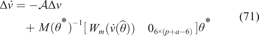
Using the fact that $\widehat{\theta }\in \text{null}\left(\mathbb{W}\left(\dot{v}\left(\widehat{\theta }\right),v,\phi ,\xi \right)\right)$ from Section 4.5.2 and the error coordinate definition (57), we can rearrange the second term in (73) to find

$\begin{array}{cc}M{\left({\theta }^{*}\right)}^{-1}& \mathbb{W}\left(\dot{v}\left(\widehat{\theta }\right),v,\phi ,\xi \right){\theta }^{*}\end{array}$

(74)

$=M{\left({\theta }^{*}\right)}^{-1}\mathbb{W}\left(\dot{v}\left(\widehat{\theta }\right),v,\phi ,\xi \right)\left({\theta }^{*}-\widehat{\theta }\right)$

(75)

$=-M{\left({\theta }^{*}\right)}^{-1}\mathbb{W}\left(\dot{v}\left(\widehat{\theta }\right),v,\phi ,\xi \right)\mathrm{\Delta }\theta .$

(76)

Substituting (76) into (73) yields

$\mathrm{\Delta }\dot{v}=-\mathcal{A}\mathrm{\Delta }v-M{\left({\theta }^{*}\right)}^{-1}\mathbb{W}\left(\dot{v}\left(\widehat{\theta }\right),v,\phi ,\xi \right)\mathrm{\Delta }\theta .$

(77)

The parameter error dynamics follow directly from the error coordinates (57), the parameter update law (64), and the assumption that the true parameters are constant, that is, ${\dot{\theta }}^{*}=0$ , thus the parameter error dynamics can be written

$\mathrm{\Delta }\stackrel{.}{\theta }=\mathrm{\Gamma }\hspace{0.17em}{\mathbb{W}}^T\left(\dot{v}\left(\widehat{\theta }\right),v,\phi ,\xi \right)\mathrm{\Delta }v.$

(78)

By defining the full error state vector for the AID as

$z\left(t\right)=\left[\begin{array}{c}\mathrm{\Delta }v\left(t\right)\\ \mathrm{\Delta }\theta \left(t\right)\end{array}\right],$

(79)

we can construct a representation of this error system using the velocity error dynamics (77) and parameter error dynamics (78):

$\begin{array}{c}\dot{z}\left(t\right)=\left[\begin{array}{cc}{M}^{-1}& 0_{6\times \left(p+a\right)}\\ 0_{\left(p+a\right)\times 6}& \mathrm{\Gamma }\end{array}\right]\left[\begin{array}{cc}-M\mathcal{A}& -\mathbb{W}\left(t,\widehat{\theta }\right)\\ \mathbb{W}{\left(t,\widehat{\theta }\right)}^T& 0_{\left(p+a\right)\times \left(p+a\right)}\end{array}\right]z\left(t\right)\end{array}$

(80)

$\begin{array}{c}=(\underset{E}{\underbrace{\left[\begin{array}{cc}{M}^{-1}& 0_{6\times \left(p+a\right)}\\ 0_{\left(p+a\right)\times 6}& \mathrm{\Gamma }\end{array}\right]}}\underset{F\left(t\right)}{\underbrace{\left[\begin{array}{cc}{0}_{6\times 6}& -\mathbb{W}\left(t,\widehat{\theta }\right)\\ \mathbb{W}{\left(t,\widehat{\theta }\right)}^T& 0_{\left(p+a\right)\times \left(p+a\right)}\end{array}\right]}}\\ +\underset{G}{\underbrace{\left[\begin{array}{cc}-\mathcal{A}& 0_{6\times \left(p+a\right)}\\ 0_{\left(p+a\right)\times 6}& 0_{\left(p+a\right)\times \left(p+a\right)}\end{array}\right]}})z\left(t\right)\end{array}$

(81)

where we adopt the notation

$\begin{array}{c}\mathbb{W}\left(t,\widehat{\theta }\right)=\mathbb{W}\left(\dot{v}\left(\widehat{\theta }\right),v,\phi ,\xi \right)\end{array}$

(82)

$\begin{array}{c}M=M\left({\theta }^{*}\right)\end{array}$

(83)

for readability. Note that the matrix

$E=E^T=\left[\begin{array}{cc}{M}^{-1}& 0_{6\times \left(p+a\right)}\\ 0_{\left(p+a\right)\times 6}& \mathrm{\Gamma }\end{array}\right]$

(84)

is block diagonal PDS,

$F\left(t\right)=-F{\left(t\right)}^T=\left[\begin{array}{cc}{0}_{6\times 6}& -\mathbb{W}\left(t,\widehat{\theta }\right)\\ \mathbb{W}{\left(t,\widehat{\theta }\right)}^T& 0_{\left(p+a\right)\times \left(p+a\right)}\end{array}\right]$

(85)

is skew-symmetric, and

$G=G^T=\left[\begin{array}{cc}-\mathcal{A}& 0_{6\times \left(p+a\right)}\\ 0_{\left(p+a\right)\times 6}& 0_{\left(p+a\right)\times \left(p+a\right)}\end{array}\right]$

(86)

is block diagonal and negative semidefinite.

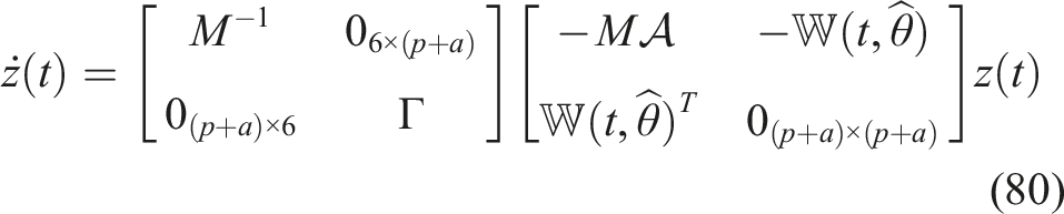
5.2 Convergence of the velocity error

Theorem 1

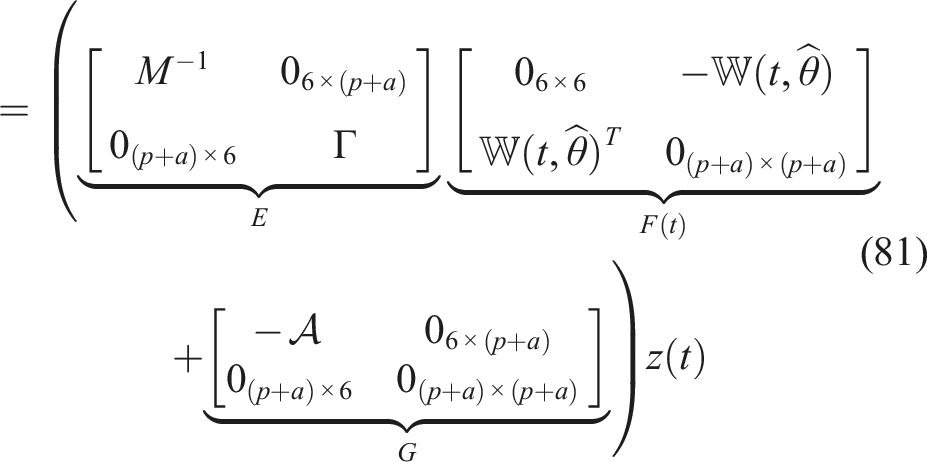
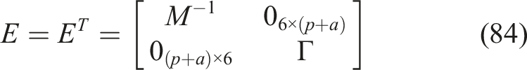
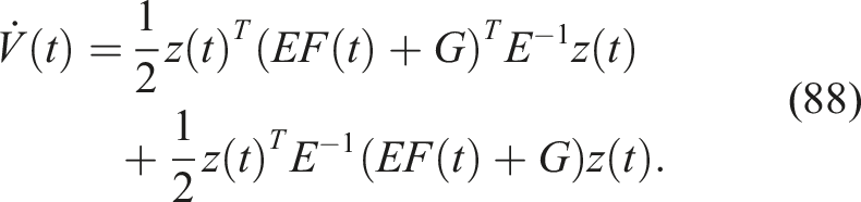
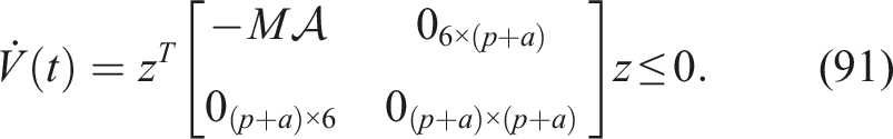
The system (80)

$\dot{z}\left(t\right)=\left[\begin{array}{cc}{M}^{-1}& 0\\ 0& \mathrm{\Gamma }\end{array}\right]\left[\begin{array}{cc}-M\mathcal{A}& -\mathbb{W}\left(t,\widehat{\theta }\right)\\ \mathbb{W}{\left(t,\widehat{\theta }\right)}^T& 0\end{array}\right]z\left(t\right)$

where z(t), M, Γ, $\mathcal{A}$ , $\mathbb{W}\left(t,\widehat{\theta }\right)$ are defined in (79, 11, 66, 65, 82) is locally uniformly stable about the set S* (61), all signals remain bounded, and lim_t→∞Δv = 0.

Proof. Consider the following Lyapunov function candidate:

$V\left(t\right)=\frac{1}{2}z{\left(t\right)}^T{E}^{-1}z\left(t\right).$

(87)

Note that $V\left(t\right)\in {\mathcal{C}}^1$ and is radially unbounded in z(t), positive definite since E⁻¹ is PDS, and equal to zero if and only if z(t) = 0. The time derivative of (87) is

$\begin{array}{cc}\dot{V}\left(t\right)& =\frac{1}{2}z{\left(t\right)}^T{\left(EF\left(t\right)+G\right)}^T{E}^{-1}z\left(t\right)\\ & +\frac{1}{2}z{\left(t\right)}^T{E}^{-1}\left(EF\left(t\right)+G\right)z\left(t\right).\end{array}$

(88)

E = E ^T and G = G ^T , so

$\dot{V}\left(t\right)=\frac{1}{2}{z}^T\left({F\left(t\right)}^T+G{E}^{-1}\right)z+\frac{1}{2}{z}^T\left(F\left(t\right)+E^{-1}G\right)z,$

(89)

and since F(t) = −F(t) ^T and E⁻¹ and G commute, we have

$\begin{array}{c}\dot{V}\left(t\right)=z^T{E}^{-1}Gz\end{array}$

(90)

$\begin{array}{c}\dot{V}\left(t\right)=z^T\left[\begin{array}{cc}-M\mathcal{A}& 0_{6\times \left(p+a\right)}\\ 0_{\left(p+a\right)\times 6}& 0_{\left(p+a\right)\times \left(p+a\right)}\end{array}\right]z\le 0.\end{array}$

(91)

This expression is negative definite in Δv and negative semidefinite in Δθ, satisfying the requirements on a Lyapunov function to show that the system (81) is uniformly stable about the set S* and that Δv and Δθ are bounded. We note that with Δθ bounded and θ* constant, it is implied that $\widehat{\theta }$ is bounded.

To show that $\mathrm{\Delta }\dot{v}$ (77) is bounded, it remains to be shown that $M{\left(\widehat{\theta }\right)}^{-1}$ is bounded. We adapt the proof in McFarland and Whitcomb (2013). Consider that ∀t > t₀, the following hold:

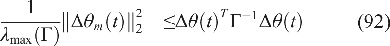
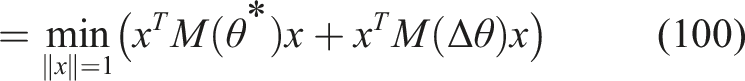
• Δθ(t) ^T Γ⁻¹θ(t) ≥ 0 from PDS of Γ

• 0 ≤ V(t) ≤ V(t₀) from (91)

• Δv(t₀) = 0 by assumption

These facts can be used to show

$\begin{array}{cc}\frac{1}{{\lambda }_{\max }\left(\mathrm{\Gamma }\right)}{\Vert \mathrm{\Delta }{\theta }_m\left(t\right)\Vert }_2^2& \le \mathrm{\Delta }\theta {\left(t\right)}^T{\mathrm{\Gamma }}^{-1}\mathrm{\Delta }\theta \left(t\right)\end{array}$

(92)

$\begin{array}{cc}& \le 2V\left(t\right)\end{array}$

(93)

$\begin{array}{cc}& \le 2V\left(t_0\right)\end{array}$

(94)

$\begin{array}{cc}& \le \mathrm{\Delta }\theta {\left(t_0\right)}^T{\mathrm{\Gamma }}^{-1}\mathrm{\Delta }\theta \left(t_0\right).\end{array}$

(95)

This implies

${\Vert \mathrm{\Delta }{\theta }_m\left(t\right)\Vert }_2^2\le {\lambda }_{\max }\left(\mathrm{\Gamma }\right)\mathrm{\Delta }\theta {\left(t_0\right)}^T{\mathrm{\Gamma }}^{-1}\mathrm{\Delta }\theta \left(t_0\right)$

(96)

and since, by assumption (60),

${\left[{\lambda }_{\max }\left(\mathrm{\Gamma }\right)\mathrm{\Delta }\theta {\left(t_0\right)}^T{\mathrm{\Gamma }}^{-1}\mathrm{\Delta }\theta \left(t_0\right)\right]}^{\frac{1}{2}}\le {\lambda }_{\min }\left(M\left({\theta }^{*}\right)\right)-ϵ,$

(97)

we can state

${\Vert \mathrm{\Delta }{\theta }_m\left(t\right)\Vert }_2^2\le {\lambda }_{\min }\left(M\left({\theta }^{*}\right)\right)-ϵ.$

(98)

Using the Rayleigh-Ritz theorem, we will show that the smallest eigenvalue of $M\left(\widehat{\theta }\right)$ is bounded away from zero as follows:

${\lambda }_{\min }\left(M\left(\widehat{\theta }\right)\right)=\underset{\Vert x\Vert =1}{\min }\left(x^{T}M\left(\widehat{\theta }\right)x\right)$

(99)

$=\underset{\Vert x\Vert =1}{\min }\left(x^{T}M\left({\theta }^{*}\right)x+x^{T}M\left(\mathrm{\Delta }\theta \right)x\right)$

(100)

$\ge \underset{\Vert x\Vert =1}{\min }\left(x^{T}M\left(\theta \right)x\right)-\underset{\Vert x\Vert =1}{\max }\left|x^{T}M\left(\mathrm{\Delta }\theta \right)x\right|.$

(101)

The second term in (101) is equal to the maximum magnitude of the eigenvalues of M(Δθ). Since M(Δθ) is symmetric, this is equivalent to its maximum singular value or ‖M(Δθ)‖₂. Furthermore, ‖M(Δθ)‖₂ ≤ ‖M(Δθ)‖ _F , and for diagonal mass matrices, ‖M(Δθ)‖ _F = ‖Δθ _m ‖₂ by definition. Thus, we have

$\begin{array}{cc}{\lambda }_{\min }\left(M\left(\widehat{\theta }\right)\right)& \ge {\lambda }_{\min }\left(M\left({\theta }^{*}\right)\right)-{\Vert M\left(\mathrm{\Delta }\theta \right)\Vert }_2\end{array}$

(102)

$\begin{array}{cc}& \ge {\lambda }_{\min }\left(M\left({\theta }^{*}\right)\right)-{\Vert M\left(\mathrm{\Delta }\theta \right)\Vert }_F\end{array}$

(103)

$\begin{array}{cc}& \ge {\lambda }_{\min }\left(M\left({\theta }^{*}\right)\right)-{\Vert \mathrm{\Delta }{\theta }_m\Vert }_2.\end{array}$

(104)

Substituting (98), we have

${\lambda }_{\min }\left(M\left(\widehat{\theta }\right)\right)\ge ϵ,$

(105)

thus $M{\left(\widehat{\theta }\right)}^{-1}$ exists and is bounded.

All signals in the right-hand side of (77) are thus shown to be bounded. This implies the time-derivative of the velocity error, $\mathrm{\Delta }\dot{v}$ , is bounded. We note that the plant acceleration $\dot{v}$ is also bounded, since all of its components are bounded (41). Since both $\dot{v}$ and $\mathrm{\Delta }\dot{v}$ are bounded, the velocity update law $\dot{\widehat{v}}$ is also bounded (68), and from bounded $\dot{\widehat{v}}$ , Δv we have bounded $\dot{v}\left(\widehat{\theta }\right)$ (63).

From (79), (87), and (91) it can easily be shown that $\mathrm{\Delta }v\in {\mathcal{L}}_2\cap {\mathcal{L}}_{\infty }$ , which together with bounded $\mathrm{\Delta }\dot{v}$ implies that lim_t→∞Δv = 0. Thus we have shown that this AID achieves (58). Regarding the parameter estimates, however, we can only conclude that Δθ is bounded, that the update law $\stackrel{.}{\widehat{\theta }}$ (64) is bounded, and that ${\lim }_{t\to \infty }\mathrm{\Delta }\stackrel{.}{\theta }={\lim }_{t\to \infty }\stackrel{.}{\widehat{\theta }}=0$ (78). Additional arguments and conditions are needed to show mathematically the convergence of $\widehat{\theta }$ to the set P(θ).

5.3. Convergence of the parameter estimate

Section 5.2 showed that lim_t→∞Δv(t) = 0 and ${\lim }_{t\to \infty }\stackrel{.}{\widehat{\theta }}\left(t\right)=0$ . This argument by itself does not show that the parameter estimate converges to the true parameter set P(θ), defined in (37). Moreover, because the set of true parameters is not defined by a single point in parameter space but rather by the set P(θ), the goal is not to show convergence of $\widehat{\theta }\left(t\right)$ to a single point (i.e., the goal is not to show that lim_t→∞Δθ(t) = 0). This Section will state conditions for and show the convergence of $\widehat{\theta }\left(t\right)$ to P(θ) (59).

The remainder of this Section is organized as follows:

• Section 5.3.1 introduces a change of coordinates to characterize $\widehat{\theta }\left(t\right)$ as the sum of two components residing in orthogonal subspaces related to P(θ).

• Section 5.3.2, then defines an equivalent error system using these coordinates.

• Finally, Section 5.3.3 shows a sufficient condition for $\widehat{\theta }\left(t\right)$ to converge to the true parameter space P(θ), that is, ${\lim }_{t\to \infty }\widehat{\theta }\left(t\right)\in P\left(\theta \right)$ .

We note that the problem of parameter convergence with respect to a unique set of true parameters is well understood for a class of linear time-varying systems, as originally reported in Morgan and Narendra (1977). To the best of our knowledge, however, we are unaware of any previously reported convergence proof applicable to the nonlinear system (80) with nullspace parameter structure.

5.3.1. Coordinate transformation

Given the set P(θ) (37), we can define the linear vector subspace P _s = P(θ) ∪ 0, with dim(P _s ) = r, and we can define an orthonormal basis {p₁, …, p _r } for P _s , as well as the matrix

$\overline{P}\triangleq \left[p_1,\dots ,p_r\right]\in {\mathbb{R}}^{\left(p+a\right)\times r}$

(106)

whose rank is r, with properties

$\begin{array}{cc}{\overline{P}}^T\overline{P}& =I_{r\times r}\end{array}$

(107)

$\begin{array}{cc}\mathbb{W}\left(\dot{v}\left({\theta }^{*}\right),v,\phi ,\xi \right)\overline{P}& =0_{6\times r}.\end{array}$

(108)

Similarly, we can define the linear vector subspace P_⊥ as the orthogonal complement of P _s , with orthonormal basis {q₁, …, q_(p+a)−r}, as well as the matrix

${\overline{P}}_{\perp }\triangleq \left[q_1,\dots ,q_{\left(p+a\right)-r}\right]\in {\mathbb{R}}^{\left(p+a\right)\times \left[\left(p+a\right)-r\right]}$

(109)

whose rank is (p + a) − r, with properties

$\begin{array}{cc}{\overline{P}}_{\perp }^T{\overline{P}}_{\perp }& =I_{\left[\left(p+a\right)-r\right]\times \left[\left(p+a\right)-r\right]}\end{array}$

(110)

$\begin{array}{cc}{\overline{P}}_{\perp }^T\overline{P}& =0_{\left[\left(p+a\right)-r\right]\times r}.\end{array}$

(111)

We note that ${\mathbb{R}}^{\left(p+a\right)}$ is the direct sum of the orthogonal subspaces P_⊥ and P _s , that is, ${\mathbb{R}}^{\left(p+a\right)}=P_{\perp }\oplus P_s$ .

We combine $\overline{P}$ and ${\overline{P}}_{\perp }$ into the orthogonal matrix

$Q\triangleq \left[\begin{array}{cc}{\overline{P}}_{\perp }& \overline{P}\end{array}\right]\in {\mathbb{R}}^{\left(p+a\right)\times \left(p+a\right)}$

(112)

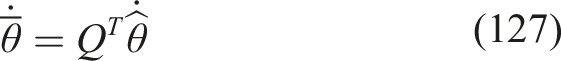
Using Q, we can perform a change of coordinates on the parameter estimate $\widehat{\theta }$ so that

$\widehat{\theta }=Q\overline{\theta }$

(113)

$\stackrel{.}{\widehat{\theta }}=Q\stackrel{.}{\overline{\theta }},$

(114)

where $\overline{\theta }\in {\mathbb{R}}^{\left(p+a\right)}$ can be decomposed into ${\overline{\theta }}_{P_{\perp }}\in {\mathbb{R}}^{\left(p+a\right)-r}$ and ${\overline{\theta }}_P\in {\mathbb{R}}^r$ , the coordinates of $\widehat{\theta }$ in P_⊥ and P, respectively:

$\overline{\theta }=\left[\begin{array}{c}{\overline{\theta }}_{P_{\perp }}\\ {\overline{\theta }}_P\end{array}\right].$

(115)

5.3.2. Equivalent error dynamics

We can obtain an expression equivalent to (73) for $\mathrm{\Delta }\dot{v}$ by factoring out $M\left(\widehat{\theta }\right)$ instead of M(θ*) and substituting (67) for $\dot{v}\left(\widehat{\theta }\right)$ in the derivation (68–73):

$\begin{array}{c}\mathrm{\Delta }\dot{v}=\dot{\widehat{v}}-\dot{v}\end{array}$

(116)

$\begin{array}{cc}& =-\mathcal{A}\mathrm{\Delta }v+\dot{v}\left(\widehat{\theta }\right)-\dot{v}\left({\theta }^{*}\right)\end{array}$

(117)

$\begin{array}{cc}& =-\mathcal{A}\mathrm{\Delta }v+\dot{v}\left(\widehat{\theta }\right)-M{\left(\widehat{\theta }\right)}^{-1}M\left(\widehat{\theta }\right)\dot{v}\left({\theta }^{*}\right)\end{array}$

(118)

$\begin{array}{cc}& =-\mathcal{A}\mathrm{\Delta }v+M{\left(\widehat{\theta }\right)}^{-1}{W}_{\dot{v}}\left(v,\phi ,\xi \right)\widehat{\theta }\\ & -M^{-1}\left(\widehat{\theta }\right)\left[\begin{array}{cc}{W}_m\left(\dot{v}\left({\theta }^{*}\right)\right)& 0_{6\times \left(\left(p+a\right)-6\right)}\end{array}\right]\widehat{\theta }\end{array}$

(119)

$\begin{array}{cc}& =-\mathcal{A}\mathrm{\Delta }v-M{\left(\widehat{\theta }\right)}^{-1}\left(\right[\begin{array}{cc}{W}_m\left(\dot{v}\left({\theta }^{*}\right)\right)& 0_{6\times \left(\left(p+a\right)-6\right)}\end{array}]\\ & -W_{\dot{v}}\left(v,\phi ,\xi \right))\widehat{\theta }\end{array}$

(120)

$\begin{array}{cc}& =-\mathcal{A}\mathrm{\Delta }v-M{\left(\widehat{\theta }\right)}^{-1}\mathbb{W}\left(\dot{v}\left({\theta }^{*}\right),v,\phi ,\xi \right)\widehat{\theta }.\end{array}$

(121)

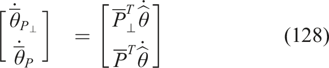
Using the coordinates ${\overline{\theta }}_{P_{\perp }},{\overline{\theta }}_P$ (113,115) for $\widehat{\theta }$ and the property (108), we have

$\begin{array}{c}\mathrm{\Delta }\dot{v}=-\mathcal{A}\mathrm{\Delta }v-M{\left(\widehat{\theta }\right)}^{-1}\mathbb{W}\left(\dot{v}\left({\theta }^{*}\right),v,\phi ,\xi \right)Q\overline{\theta }\end{array}$

(122)

$\begin{array}{cc}& =-\mathcal{A}\mathrm{\Delta }v\\ & -M{\left(\widehat{\theta }\right)}^{-1}\mathbb{W}\left(\dot{v}\left({\theta }^{*}\right),v,\phi ,\xi \right)\left({\overline{P}}_{\perp }{\overline{\theta }}_{P_{\perp }}+\overline{P}{\overline{\theta }}_P\right)\end{array}$

(123)

$\begin{array}{cc}& =-\mathcal{A}\mathrm{\Delta }v-M{\left(\widehat{\theta }\right)}^{-1}\mathbb{W}\left(\dot{v}\left({\theta }^{*}\right),v,\phi ,\xi \right){\overline{P}}_{\perp }{\overline{\theta }}_{P_{\perp }},\end{array}$

(124)

and defining the term

$W_{\perp }\left(t\right)\triangleq M^{-1}\left(\widehat{\theta }\left(t\right)\right)\mathbb{W}\left(\dot{v}\left({\theta }^{*},t\right),v\left(t\right),\phi \left(t\right),\xi \left(t\right)\right){\overline{P}}_{\perp },$

(125)

we can rewrite (124) as

$\mathrm{\Delta }\dot{v}=-\mathcal{A}\mathrm{\Delta }v-W_{\perp }{\overline{\theta }}_{P_{\perp }}.$

(126)

We also have the derivative of $\overline{\theta }$ , given by (114)

$\begin{array}{cc}\stackrel{.}{\overline{\theta }}& =Q^T\stackrel{.}{\widehat{\theta }}\end{array}$

(127)

$\begin{array}{cc}\left[\begin{array}{c}{\stackrel{.}{\overline{\theta }}}_{P_{\perp }}\\ {\stackrel{.}{\overline{\theta }}}_P\end{array}\right]& =\left[\begin{array}{c}{\overline{P}}_{\perp }^T\stackrel{.}{\widehat{\theta }}\\ {\overline{P}}^T\stackrel{.}{\widehat{\theta }}\end{array}\right]\end{array}$

(128)

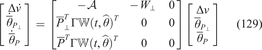
From (64, 126), this results in the full transformed system

$\left[\begin{array}{c}\mathrm{\Delta }\dot{v}\\ {\stackrel{.}{\overline{\theta }}}_{P_{\perp }}\\ {\stackrel{.}{\overline{\theta }}}_P\end{array}\right]=\left[\begin{array}{ccc}-\mathcal{A}& -W_{\perp }& 0\\ {\overline{P}}_{\perp }^T\mathrm{\Gamma }\mathbb{W}{\left(t,\widehat{\theta }\right)}^T& 0& 0\\ {\overline{P}}^T\mathrm{\Gamma }\mathbb{W}{\left(t,\widehat{\theta }\right)}^T& 0& 0\end{array}\right]\left[\begin{array}{c}\mathrm{\Delta }v\\ {\overline{\theta }}_{P_{\perp }}\\ {\overline{\theta }}_P\end{array}\right]$

(129)

in which we have partially isolated the velocity error dynamics $\mathrm{\Delta }\dot{v}$ from the coordinates ${\overline{\theta }}_P$ of $\widehat{\theta }$ that already belong to the true parameter set P(θ), although a nonlinear state dependence remains in W_⊥ through $\widehat{\theta }$ (125).

5.3.3. Convergence of $\mathrm{\Delta }\dot{v}\left(t\right)$

Before showing a sufficient condition for ${\lim }_{t\to \infty }\widehat{\theta }\in P\left(\theta \right)$ , we state and prove the following useful lemma.

Lemma 1

Given the system described in Theorem 1 and the transformed system (129), then

$\underset{t\to \infty }{\lim }{W}_{\perp }\left(t\right){\overline{\theta }}_{P_{\perp }}\left(t\right)=0.$

(130)

Proof. One conclusion of Theorem 1 is that lim_t→∞Δv(t) = 0. We apply this result to the transformed system (129) to find

$\begin{array}{c}\underset{t\to \infty }{\lim }\mathrm{\Delta }\dot{v}\left(t\right)=\underset{t\to \infty }{\lim }\left(-\mathcal{A}\mathrm{\Delta }v\left(t\right)-W_{\perp }\left(t\right){\overline{\theta }}_{P_{\perp }}\left(t\right)\right)\end{array}$

(131)

$\begin{array}{cc}& =\underset{t\to \infty }{\lim }-W_{\perp }\left(t\right){\overline{\theta }}_{P_{\perp }}\left(t\right).\end{array}$

(132)

By Barbalat’s Lemma (Appendix B.1), if lim_t→∞Δv(t) is finite and $\mathrm{\Delta }\dot{v}\left(t\right)$ is uniformly continuous (UC) with respect to time, then ${\lim }_{t\to \infty }\mathrm{\Delta }\dot{v}\left(t\right)=0$ . We show the details regarding UC of $\mathrm{\Delta }\dot{v}$ in Appendix B.2. With the conditions of Barbalat’s Lemma satisfied for each element in the vector Δv(t), we conclude that

$\underset{t\to \infty }{\lim }\mathrm{\Delta }\dot{v}\left(t\right)=\underset{t\to \infty }{\lim }-W_{\perp }\left(t\right){\overline{\theta }}_{P_{\perp }}\left(t\right)=0,$

(133)

and this completes the proof of Lemma 1.

Examining the structure of W_⊥ (125), we observe that the nullspace of $M{\left(\widehat{\theta }\right)}^{-1}\mathbb{W}\left(\dot{v}\left({\theta }^{*}\right),v,\phi ,\xi \right)$ at any time t always contains P(θ) (37), but that ${\overline{P}}_{\perp }$ is by definition a matrix of basis vectors orthogonal to P(θ); thus P(θ) is removed from null(W_⊥(t)). Intuitively, if W_⊥(t) has no persistent non-trivial nullspace, the only way to satisfy (130) is for ${\overline{\theta }}_{P_{\perp }}\left(t\right)$ to converge to zero. We will use this argument in the following theorem, which presents a sufficient condition for convergence of $\widehat{\theta }$ to P(θ).

5.3.4. Convergence of $\widehat{\theta }\left(t\right)$ to the true parameter set P(θ)

Theorem 2

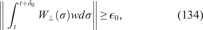
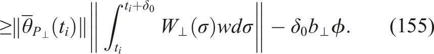
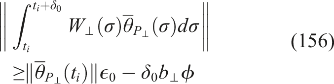
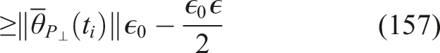
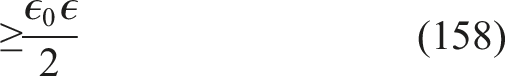
For the system described by Theorem 1 and W_⊥(t) defined in (125), if there exist ϵ₀, δ₀ > 0 such that for any t ≥ t₀ and any unit vector $w\in {\mathbb{R}}^{\left(p+a\right)-r}$ ,

$\Vert {\int }_t^{t+{\delta }_0}{W}_{\perp }\left(\sigma \right)wd\sigma \Vert \ge {ϵ}_0,$

(134)

then ${\lim }_{t\to \infty }\widehat{\theta }\left(t\right)\in P\left(\theta \right)$ .

In other words, if W_⊥(t) is persistently exciting (PE) as defined in (134), then $\widehat{\theta }\left(t\right)$ converges to the true parameter set P(θ) (37), and the full state z(t) converges to the set S (62).

Proof. It suffices to show that ${\lim }_{t\to \infty }{\overline{\theta }}_{P_{\perp }}\left(t\right)=0$ , which implies ${\lim }_{t\to \infty }\widehat{\theta }\left(t\right)\in P\left(\theta \right)$ . We prove this theorem by contradiction. First, we state assumptions and conditions of the theorem in Part 1. In Part 2, we suppose that ${\lim }_{t\to \infty }{\overline{\theta }}_{P_{\perp }}\left(t\right)\ne 0$ , which we will later show to be a contradiction. In Part 3, we show that “when Δv is small, ${\overline{\theta }}_{P_{\perp }}$ is flat,” using the approach described in Morgan and Narendra (1977). Finally, in Part 4 we use the flatness property and the PE condition (134) find a result that contradicts Lemma 1.

• Let all of the assumptions in Section 5 be satisfied such that Theorem 1 is true, including that lim_t→∞Δv(t) = 0.

• Let the PE condition in (134) be satisfied.

• Lemma 1 showed that ${\lim }_{t\to \infty }{W}_{\perp }\left(t\right){\overline{\theta }}_{P_{\perp }}\left(t\right)=0$ .

• We also define the bounds b, b_⊥ > 0 such that

$\begin{array}{cc}& \forall t\ge t_0,b_{\perp }\ge \Vert W_{\perp }\left(t\right)\Vert \end{array}$

(135)

$\begin{array}{cc}& \forall t\ge t_0,b\ge \Vert \mathbb{W}\left(t,\widehat{\theta }\right)\Vert .\end{array}$

(136)

These bounds exist since $\mathbb{W}\left(\dot{v}\left(\widehat{\theta }\left(t\right)\right),v,\phi ,\xi \right)$ is a bounded function of $\dot{v}\left(\widehat{\theta }\right),v,\phi ,\xi$ , whose boundedness has been discussed in Section 5.2, and

$\Vert W_{\perp }\left(t\right)\Vert \le \Vert M{\left(\widehat{\theta }\right)}^{-1}\Vert \Vert \mathbb{W}\left(t,{\theta }^{*}\right)\Vert \Vert {\overline{P}}_{\perp }\Vert$

(137)

where $M{\left(\widehat{\theta }\right)}^{-1}$ and $\dot{v}\left({\theta }^{*}\right)$ were shown to exist and be bounded in Section 5.2, $\mathbb{W}\left(t,{\theta }^{*}\right)=\mathbb{W}\left(\dot{v}\left({\theta }^{*}\right),v,\phi ,\xi \right)$ is thus a bounded function of bounded functions, and $\Vert {\overline{P}}_{\perp }\Vert =1$ .

Let us suppose that ${\lim }_{t\to \infty }{\overline{\theta }}_{P_{\perp }}\left(t\right)\ne 0$ . Then there exists an ϵ > 0 and an unbounded sequence of times ${\left\{t_i\right\}}_{i=1,\dots ,\infty }$ such that $\Vert {\overline{\theta }}_{P_{\perp }}\left(t_i\right)\Vert \ge ϵ$ .

We will show that “when Δv is small, ${\overline{\theta }}_{P_{\perp }}$ is flat” using an approach included in the proof of Sublemma 2 in Morgan and Narendra (1977). Given T′, ϕ > 0, ∃ϵ′ > 0 such that if ∥Δv(t)∥ ≤ ϵ′ ∀t ∈ [t _i , t _i + T′], then

$\Vert {\overline{\theta }}_{P_{\perp }}\left(t\right)-{\overline{\theta }}_{P_{\perp }}\left(t_i\right)\Vert \le \varphi \forall t\in \left[t_i,t_i+T^{\prime }\right].$

(138)

To verify this, given a T′ and ϕ, we set

${ϵ}^{\prime }=\frac{\varphi }{T^{\prime }{\lambda }_{\max }\left(\mathrm{\Gamma }\right)b}$

(139)

and observe that, ∀t ∈ [t _i , t _i + T′], using the expression for ${\stackrel{.}{\overline{\theta }}}_{P_{\perp }}$ in (129), the fact that $\Vert {\overline{P}}_{\perp }\Vert =1$ , and the bound b (136),

$\begin{array}{cc}\Vert {\overline{\theta }}_{P_{\perp }}\left(t\right)& -{\overline{\theta }}_{P_{\perp }}\left(t_i\right)\Vert =\Vert {\int }_{t_i}^t{\stackrel{.}{\overline{\theta }}}_{P_{\perp }}\left(\sigma \right)d\sigma \Vert \end{array}$

(140)

$\begin{array}{cc}& \le \Vert {\int }_{t_i}^t{\overline{P}}_{\perp }\mathrm{\Gamma }\mathbb{W}\left(\sigma ,\widehat{\theta }\right)\mathrm{\Delta }v\left(\sigma \right)d\sigma \Vert \end{array}$

(141)

$\begin{array}{cc}& \le {\int }_{t_i}^t\Vert {\overline{P}}_{\perp }\Vert \Vert \mathrm{\Gamma }\Vert \Vert \mathbb{W}\left(\sigma ,\widehat{\theta }\right)\Vert \Vert \mathrm{\Delta }v\left(\sigma \right)\Vert d\sigma \end{array}$

(142)

$\begin{array}{cc}& \le {\int }_{t_i}^t{\lambda }_{\max }\left(\mathrm{\Gamma }\right)b{ϵ}^{\prime }d\sigma \end{array}$

(143)

$\begin{array}{cc}& \le \left(t-t_i\right){\lambda }_{\max }\left(\mathrm{\Gamma }\right)b{ϵ}^{\prime }\end{array}$

(144)

$\begin{array}{cc}& \le T^{\prime }{\lambda }_{\max }\left(\mathrm{\Gamma }\right)b{ϵ}^{\prime }\end{array}$

(145)

$\begin{array}{cc}& \le \varphi .\end{array}$

(146)

Since lim_t→∞Δv(t) = 0, for any ϵ′ > 0 we can always find a t′ ≥ t₀ such that ∥Δv(t)∥ ≤ ϵ′ ∀t ≥ t′. Thus using ϵ₀ from the PE condition (134), ϵ from the assumption made in Part 2, and the bound b_⊥ (135), we can choose

$\begin{array}{c}\varphi =\frac{{ϵ}_0ϵ}{2{\delta }_0{b}_{\perp }}\end{array}$

(147)

$\begin{array}{c}{T}^{\prime }={\delta }_0\end{array}$

(148)

and find a t′ ≥ t₀ such that the flatness property (138) holds for each interval [t _i , t _i + δ₀] where t _i ≥ t′.

We will now show that for each t _i ≥ t′, there is a t _j ∈ [t _i , t _i + δ₀] where $\Vert W_{\perp }\left(t_j\right){\overline{\theta }}_{P_{\perp }}\left(t_j\right)\Vert >0$ . For each t _i ≥ t′, we use the reverse triangle inequality and the flatness property (138) to show:

$\begin{array}{cc}& \Vert {\int }_{t_i}^{t_i+{\delta }_0}{W}_{\perp }\left(\sigma \right){\overline{\theta }}_{P_{\perp }}\left(t_i\right)d\sigma \Vert \\ & -\Vert {\int }_{t_i}^{t_i+{\delta }_0}{W}_{\perp }\left(\sigma \right){\overline{\theta }}_{P_{\perp }}\left(\sigma \right)d\sigma \Vert \\ & \le \Vert {\int }_{t_i}^{t_i+{\delta }_0}{W}_{\perp }\left(\sigma \right)\left[{\overline{\theta }}_{P_{\perp }}\left(t_i\right)-{\overline{\theta }}_{P_{\perp }}\left(\sigma \right)\right]d\sigma \Vert \end{array}$

(149)

$\begin{array}{cc}& \le {\int }_{t_i}^{t_i+{\delta }_0}\Vert W_{\perp }\left(\sigma \right)\Vert \Vert {\overline{\theta }}_{P_{\perp }}\left(t_i\right)-{\overline{\theta }}_{P_{\perp }}\left(\sigma \right)\Vert d\sigma \end{array}$

(150)

$\begin{array}{cc}& \le {\int }_{t_i}^{t_i+{\delta }_0}{b}_{\perp }\varphi d\sigma \end{array}$

(151)

$\begin{array}{cc}& \le {\delta }_0{b}_{\perp }\varphi ,\end{array}$

(152)

We rearrange (152) and choose the unit vector in the PE condition (134) to be

$w\triangleq \frac{{\overline{\theta }}_{P_{\perp }}\left(t_i\right)}{\Vert {\overline{\theta }}_{P_{\perp }}\left(t_i\right)\Vert },$

(153)

so that

$\begin{array}{cc}& \Vert {\int }_{t_i}^{t_i+{\delta }_0}{W}_{\perp }\left(\sigma \right){\overline{\theta }}_{P_{\perp }}\left(\sigma \right)d\sigma \Vert \\ & \ge \Vert {\int }_{t_i}^{t_i+{\delta }_0}{W}_{\perp }\left(\sigma \right){\overline{\theta }}_{P_{\perp }}\left(t_i\right)d\sigma \Vert -{\delta }_0{b}_{\perp }\varphi \end{array}$

(154)

$\begin{array}{cc}& \ge \Vert {\overline{\theta }}_{P_{\perp }}\left(t_i\right)\Vert \Vert {\int }_{t_i}^{t_i+{\delta }_0}{W}_{\perp }\left(\sigma \right)wd\sigma \Vert -{\delta }_0{b}_{\perp }\varphi .\end{array}$

(155)

We now invoke the lower bound in the PE condition (134), substitute our choice of ϕ (147), and recall the assumption made in Part 2 that $\Vert {\overline{\theta }}_{P_{\perp }}\left(t_i\right)\Vert \ge ϵ$ . This results in:

$\begin{array}{cc}& \Vert {\int }_{t_i}^{t_i+{\delta }_0}{W}_{\perp }\left(\sigma \right){\overline{\theta }}_{P_{\perp }}\left(\sigma \right)d\sigma \Vert \\ & \ge \Vert {\overline{\theta }}_{P_{\perp }}\left(t_i\right)\Vert {ϵ}_0-{\delta }_0{b}_{\perp }\varphi \end{array}$

(156)

$\begin{array}{cc}& \ge \Vert {\overline{\theta }}_{P_{\perp }}\left(t_i\right)\Vert {ϵ}_0-\frac{{ϵ}_0ϵ}{2}\end{array}$

(157)

$\begin{array}{cc}& \ge \frac{{ϵ}_0ϵ}{2}\end{array}$

(158)

$\begin{array}{cc}& >0.\end{array}$

(159)

Furthermore, we have

$\begin{array}{c}{\int }_{t_i}^{t_i+{\delta }_0}\Vert W_{\perp }\left(\sigma \right){\overline{\theta }}_{P_{\perp }}\left(\sigma \right)\Vert d\sigma \\ \ge \Vert {\int }_{t_i}^{t_i+{\delta }_0}{W}_{\perp }\left(\sigma \right){\overline{\theta }}_{P_{\perp }}\left(\sigma \right)d\sigma \Vert \end{array}$

(160)

$\begin{array}{cc}& >0.\end{array}$

(161)

By the mean value theorem for integrals, there must be a t _j ∈ [t _i , t _i + δ₀] where

${\int }_{t_i}^{t_i+{\delta }_0}\Vert W_{\perp }\left(\sigma \right){\overline{\theta }}_{P_{\perp }}\left(\sigma \right)\Vert d\sigma =\Vert W_{\perp }\left(t_j\right){\overline{\theta }}_{P_{\perp }}\left(t_j\right)\Vert {\delta }_0,$

(162)

and therefore from (161, 162)

$\Vert W_{\perp }\left(t_j\right){\overline{\theta }}_{P_{\perp }}\left(t_j\right)\Vert {\delta }_0>0$

(163)

$\Vert W_{\perp }\left(t_j\right){\overline{\theta }}_{P_{\perp }}\left(t_j\right)\Vert >0.$

(164)

Thus, we have found an unbounded sequence of times ${\left\{t_j\right\}}_{j=1,\dots ,\infty }$ where $\Vert W_{\perp }\left(t_j\right){\overline{\theta }}_{P_{\perp }}\left(t_j\right)\Vert >0$ , which contradicts Lemma 1 and implies that the assumption ${\lim }_{t\to \infty }{\overline{\theta }}_{P_{\perp }}\left(t\right)\ne 0$ must be false. Therefore ${\lim }_{t\to \infty }{\overline{\theta }}_{P_{\perp }}\left(t\right)=0$ , which is equivalent to ${\lim }_{t\to \infty }\widehat{\theta }\left(t\right)\in P\left(\theta \right)$ .

Together with the conclusion in the proof of Theorem one that lim_t→∞Δv(t) = 0, we have shown a sufficient condition for convergence of the full state z(t) to S, thereby achieving the goals (58,59) of this AID.

6. Simulation results

We report simulation results in which the “true” parameters of the simulated plant were chosen to match approximately those of the JHU Iver3 AUV. We include this simulation study to demonstrate that the AID achieves parameter estimate convergence to the true parameter set. Since the true parameter set of the Iver3 is unknown, we are unable to verify convergence of the parameter estimates to the “true” parameter set in the experimental results.

For this study, we simulated 5000 seconds of plant motion for the AID process. All available control inputs were excited in open loop to achieve the PE condition (134). A summary of the input signals is provided in Table 1. The set of adaptation gains used in the simulation study are listed in Table 2. We note that with different gain values, it may be possible to achieve more rapid parameter convergence, and that the selection of adaptation gains is an open problem in adaptive systems theory.

Table 1.

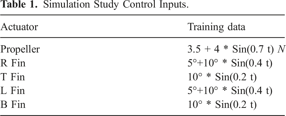
Simulation Study Control Inputs.

Actuator	Training data
Propeller	3.5 + 4 * Sin(0.7 t) N
R Fin	5°+10° * Sin(0.4 t)
T Fin	10° * Sin(0.2 t)
L Fin	5°+10° * Sin(0.4 t)
B Fin	10° * Sin(0.2 t)

Table 2.

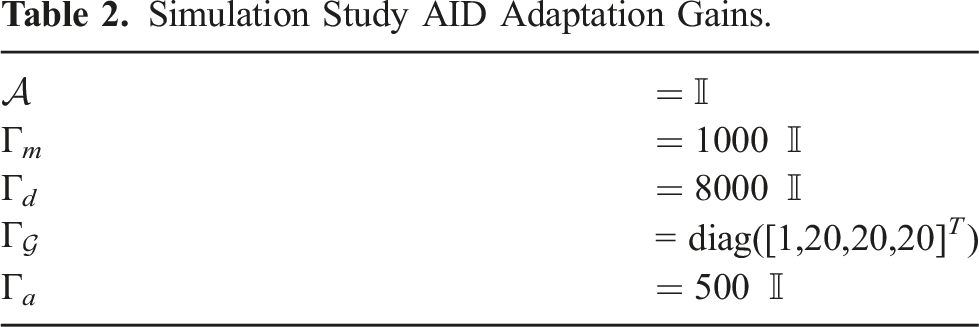
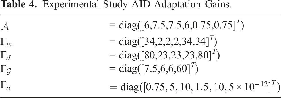
Simulation Study AID Adaptation Gains.

$\mathcal{A}$	$=\mathbb{I}$
Γ m	$=1000\mathbb{I}$
Γ d	$=8000\mathbb{I}$
${\mathrm{\Gamma }}_{\mathcal{G}}$	= diag([1,20,20,20] T )
Γ a	$=500\mathbb{I}$

Gaussian noise was added to the attitude and velocity signals to mimic the expected measurement noise of the JHU Iver3 AUV sensor suite. All sensors were assumed to be operating at the same frequency, 10 Hz, which is the sampling frequency of the JHU Iver3’s actual MicroStrain 3DM-GX5-25 attitude and heading reference sensor (AHRS). The specific noise characteristics used in this simulation study are provided in Table 3. These values were determined from manufacturer-provided data sheets and bench-top testing.

Table 3.

Measurement Sources, Accuracies, and Usage in the Reported Results.

		Measurement	Simulation	Experimental	Experimental
State	Source	Standard Deviation	Results	Results (training)	Results (validation)
Attitude	MicroStrain MSF	0.25°	X	X
Angular velocity	MicroStrain MST	0.1°/s		X
Angular velocity	KVH 1775 FOG	0.01°/s	X		X
Trans velocity	RDI 600 kHz DVL	1.3 cm/s	X	X	X

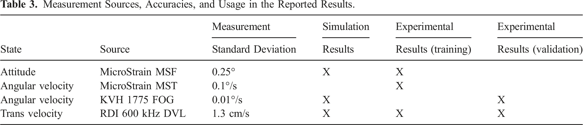
Figure 1, shows that the estimated parameters converge to “true” parameters in simulation, provided that the PE condition (134) defined in Section 5.3 is satisfied. We note that in order to compute a parameter error between the estimated parameters and the non-unique set of “true” parameters, we employed a scaling factor with respect to a single known parameter.

Figure 1.

Simulation Study: Difference between true and estimated parameters (Y-Axis) versus time in seconds (X-axis). This Figure shows that the AID-estimated parameters converge to the true parameter set in simulation when a PE condition is satisfied.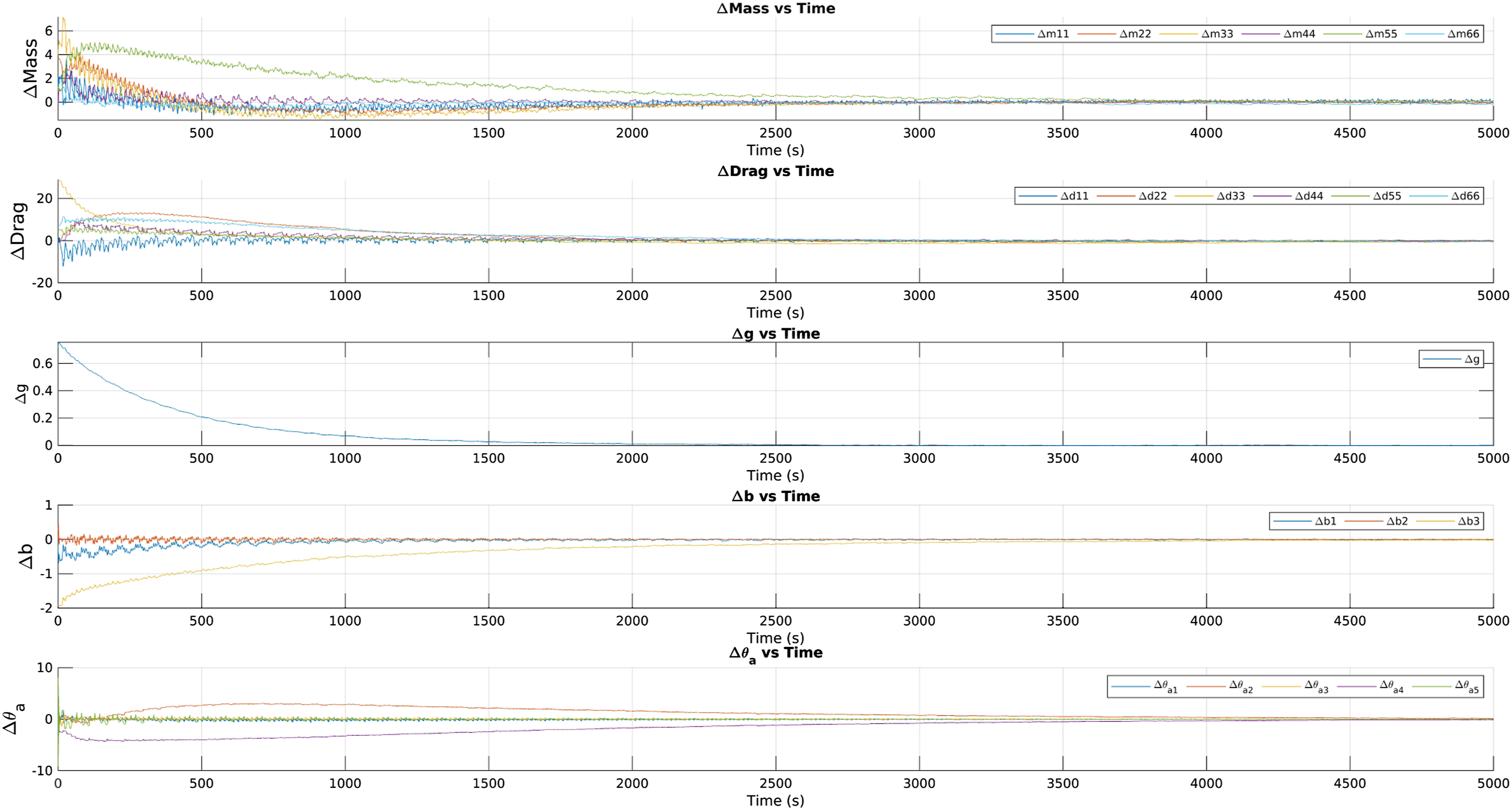

7. Experimental results

This section reports the results of three at-sea field trials to evaluate experimentally the adaptive identification (AID) parameter estimator reported above. We utilized experimental data obtained with JHU’s Iver3 AUV (L3 OceanServer, Fall River, MA, USA), shown in Figure 2. We deployed the JHU Iver3 AUV in the Chesapeake Bay, MD, on November 11, 2019, and we report data from three dives (Dive 86, 87, and 88), which are described in Section 7.1.

Figure 2.

The Iver3 AUV is an underactuated AUV whose control authority is provided by the commanded rotational speed of its ducted propeller and commanded angles for the four red/yellow tail fins, all located at the stern of the vehicle. The 100 m depth-rated Iver3 AUV is one of several commercially available small AUVs designed for oceanographic survey operations including biological, physical-oceanographic, and bathymetric survey missions.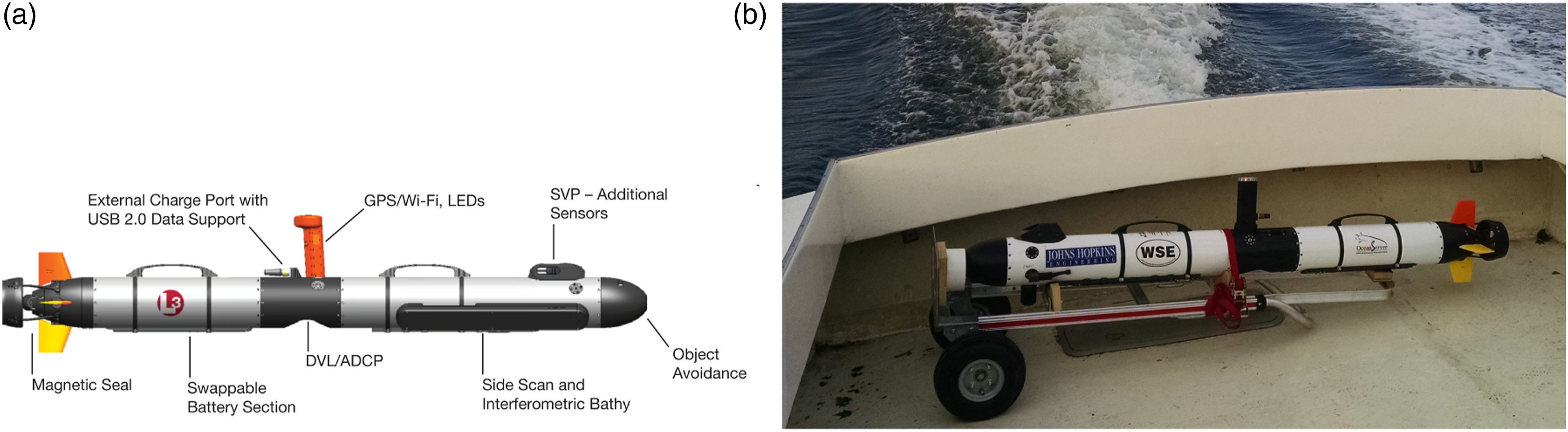

For these experiments, the Iver3 AUV was operating under “waypoint following” control, wherein the user entered a set of pre-programmed waypoints and the Iver3 proprietary controller determined the specific control inputs required to follow the waypoints.

To estimate the parameters for the Iver3 AUV using the AID, we used signals from a MicroStrain 3DM-GX5-25 (Parker LORD MicroStrain, Willston, VT, USA) which is a microelectromechanical systems (MEMS) AHRS, for the attitude and angular rate, and a Teledyne RDI Explorer (Teledyne RDInstruments, Poway, CA, USA) 600 kHz phased-array Doppler velocity log (DVL) for the translational velocity. The RDI DVL is part of the standard sensor suite on the Iver3 AUV installed by the manufacturer; the MicroStrain AHRS was integrated into the nose cone of the Iver3 AUV by the authors. An auxiliary inertial measurement unit (IMU) sensor, a KVH 1775 (KVH Industries, Middletown, RI, USA) fiber-optic gyroscope (FOG), which measures angular rate, was installed inside the Iver3 for these experimental trials. The KVH FOG, which is more accurate than the MicroStrain MEMS gyro, was used as an external source of “ground truth” for the angular rate DOFs during validation. The sensors used for AID and their noise characteristics are listed in Table 3.

7.1. Dive mission plans

Three experimental trials were conducted:

• Dive 86 was a waypoint-following undulate mission with relatively high variation in motion.

• Dive 87 was a waypoint-following mission with a lawnmower pattern at constant depth

• Dive 88 was the same mission as Dive 86.

An overview of the three dives is given in Figure 3. While it may have been ideal to utilize open-loop control signals for these experiments, as we did in simulation, it would have been infeasible in practice when operating in open water with an untethered UV. Instead, we utilized the manufacturer-provided mission planning tool to enter pre-programmed waypoints for the proprietary controller to follow.

Figure 3.

Overview of the three dives conducted in the Chesapeake Bay using the Iver3. The translational position during each dive as estimated by the front seat of the Iver3 is shown above in blue. The depth profile of each dive is shown below in red.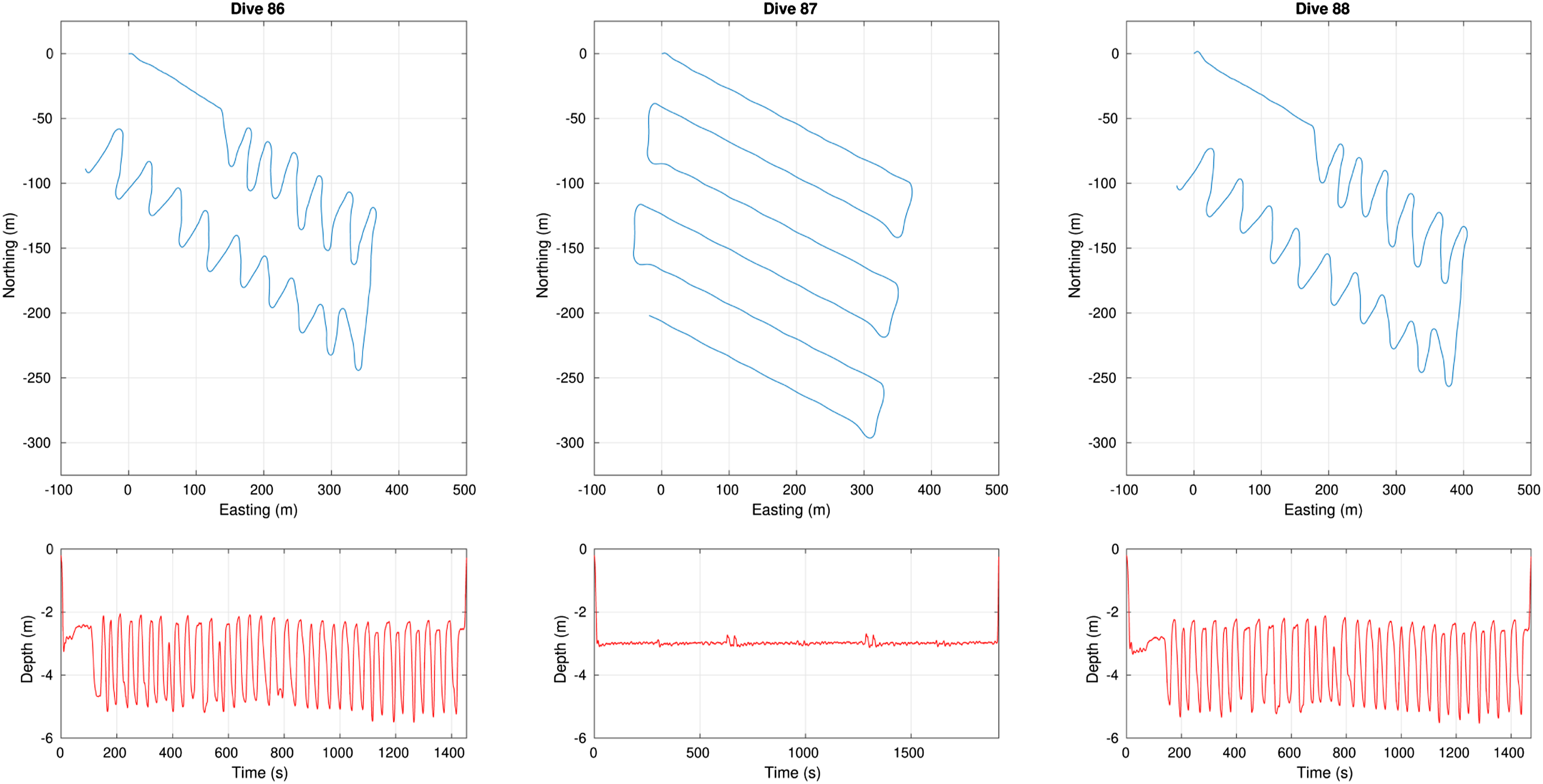

The waypoint-following undulate missions (Dives 86 and 88) were designed to excite the UV dynamics. The UV attempted to follow a series of zig-zagging waypoints while constantly undulating between 1 m and 5 m depths at a fixed 20° pitch angle. The constant-depth lawnmower mission (Dive 87), where the UV followed a series of waypoints in a rectangular grid, was designed to emulate typical seafloor mapping with a multi-beam sonar.

While Dives 86 and 88 employed the same mission, the control inputs determined by the manufacturer’s controller were not identical. External factors such as the UV’s initial position and the ambient water current resulted in different control inputs when following the same mission waypoints.

7.2. Experimental evaluation methodology

Our approach to evaluating the performance of the new AID was a “training and validation” procedure, in which we identified the parameters using the AID algorithm on experimental data from one dive, termed the “training” data, and then used those parameters in forward simulations of different dives, termed the “validation” data. We compared the resulting 6-DOF simulated model velocities to the actual experimentally-observed 6-DOF vehicle velocities. Since the control algorithms of the Iver3 feedback control system are not disclosed by the manufacturer, we used the experimentally-recorded control signals as inputs to the simulation of each dive. We also performed a “self-validation” procedure by computing a forward simulation of the training dive using its own estimated parameters.

The Iver3 AUV control inputs (fin angles and propeller angular velocity) and relevant components of the vehicle state (attitude, translational velocity, and angular velocity) were logged and time-stamped in real-time to the Iver3 AUV’s on-board CPU during the experimental trials. These data were used in post-processing to evaluate the performance of the proposed AID approach. No filtering of any sensor signal was used, the adaptation gains were held constant across all simulations, and the nonlinear differential equations which make up the AID were evaluated using simple Euler integration.

This AID method is well suited for online parameter estimation—assuming that the programming implementation is capable of handling asynchronous sensor readings, the sensor alignments are calibrated, and suitable adaptation gains are chosen. The appropriate adaptation gains can be found using simulation studies or data from previous experiments.

7.2.1. Adaptation gains

During the training procedure, we empirically selected adaptation gains. The adaptation gains were then held constant throughout the self-validation and validation procedure for all dives reported below. We note that the AID reported here is not particularly sensitive to the choice of adaptation gains; that is, small changes in the magnitude of a gain did not result in large changes in performance of the AID.

The adaptation gains for the AID were tuned to maximize performance on the training data set, Dive 86, with the AID active only when the UV was fully submerged. We found Dive 86 to contain over 24 uninterrupted minutes of maneuvering below the surface. The adaptation gains are given in Table 4.

Table 4.

Experimental Study AID Adaptation Gains.

$\mathcal{A}$	= diag([6,7.5,7.5,6,0.75,0.75] T )
Γ m	= diag([34,2,2,2,34,34] T )
Γ d	= diag([80,23,23,23,80] T )
${\mathrm{\Gamma }}_{\mathcal{G}}$	= diag([7.5,6,6,60] T )
Γ a	$=\text{diag}\left({\left[\mathrm{0.75,5,10,1.5,10,5}\times {10}^{-12}\right]}^T\right)$

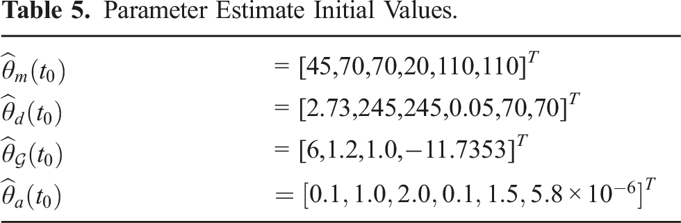
7.2.2. AID initialization

The parameter estimates for the AID were initialized to values given in Table 5.

Table 5.

Parameter Estimate Initial Values.

${\widehat{\theta }}_m\left(t_0\right)$	= [45,70,70,20,110,110] T
${\widehat{\theta }}_d\left(t_0\right)$	= [2.73,245,245,0.05,70,70] T
${\widehat{\theta }}_{\mathcal{G}}\left(t_0\right)$	= [6,1.2,1.0,−11.7353] T
${\widehat{\theta }}_a\left(t_0\right)$	$={\left[\mathrm{0.1,1.0,2.0,0.1,1.5,5.8}\times {10}^{-6}\right]}^T$

7.3. AID performance

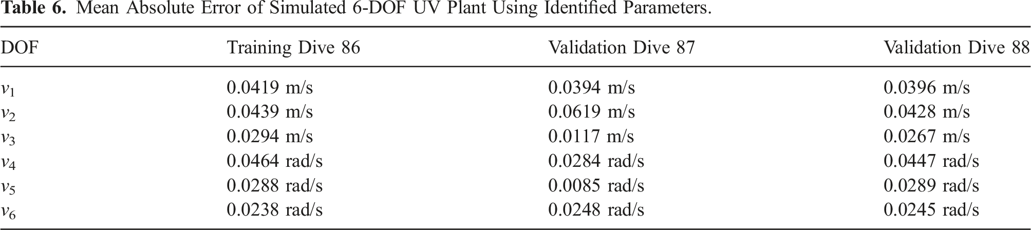
We report the performance of the AID as the mean absolute error (MAE), where the error is the difference between the simulated plant velocity resulting from the AID parameters and the velocity measured via the DVL and KVH gyro.

Table 6 reports the MAE when using the parameters estimated from the data of Dive 86 (the “training data”) on a forward simulation of the same dive and of Dives 87 and 88 (the “validation data”). A plot of the body velocity during the validation of Dive 88 is shown in Figure 4.

Table 6.

Mean Absolute Error of Simulated 6-DOF UV Plant Using Identified Parameters.

DOF	Training Dive 86	Validation Dive 87	Validation Dive 88
v 1	0.0419 m/s	0.0394 m/s	0.0396 m/s
v 2	0.0439 m/s	0.0619 m/s	0.0428 m/s
v 3	0.0294 m/s	0.0117 m/s	0.0267 m/s
v 4	0.0464 rad/s	0.0284 rad/s	0.0447 rad/s
v 5	0.0288 rad/s	0.0085 rad/s	0.0289 rad/s
v 6	0.0238 rad/s	0.0248 rad/s	0.0245 rad/s

Figure 4.

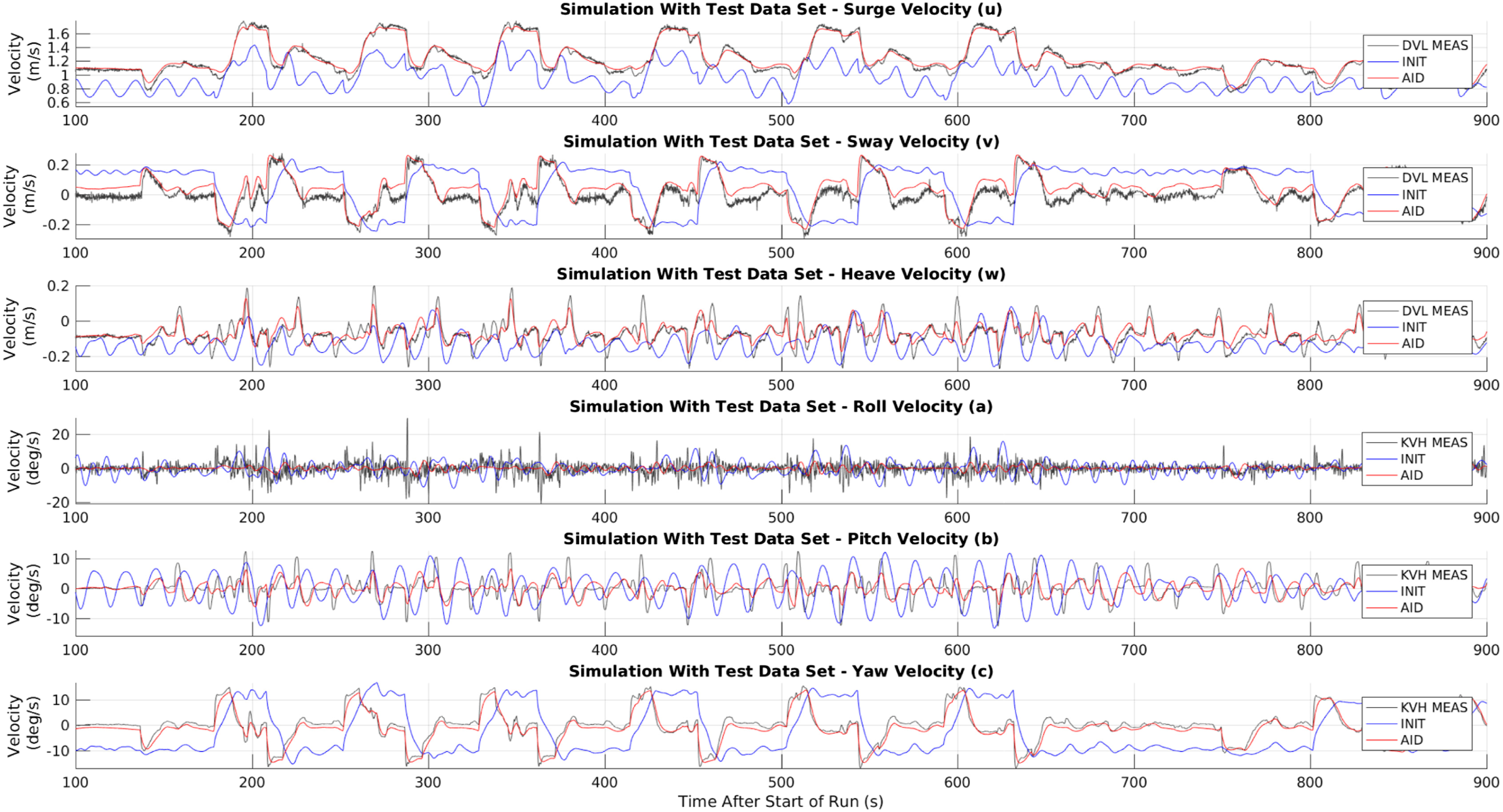
Validation results of Dive 88 using parameters identified during Dive 86. Gray traces are (unfiltered) translational and rotational velocities as measured by the DVL and KVH gyroscope. Blue traces are the plant velocities in forward simulation using the parameters as they were initialized in the AID. Red traces are plant velocities in forward simulation using the parameters identified via the new AID method.

The parameter set $\widehat{\theta }$ that was found after training on Dive 86 is reported in Table 7. As explained in Section 4.3, the dynamics of the AID plant converges to that of the real plant, but the true parameter set is not unique. Moreover, this parameter set is only applicable to the particular parameterization of the plant and actuator model satisfying (34).

Table 7.

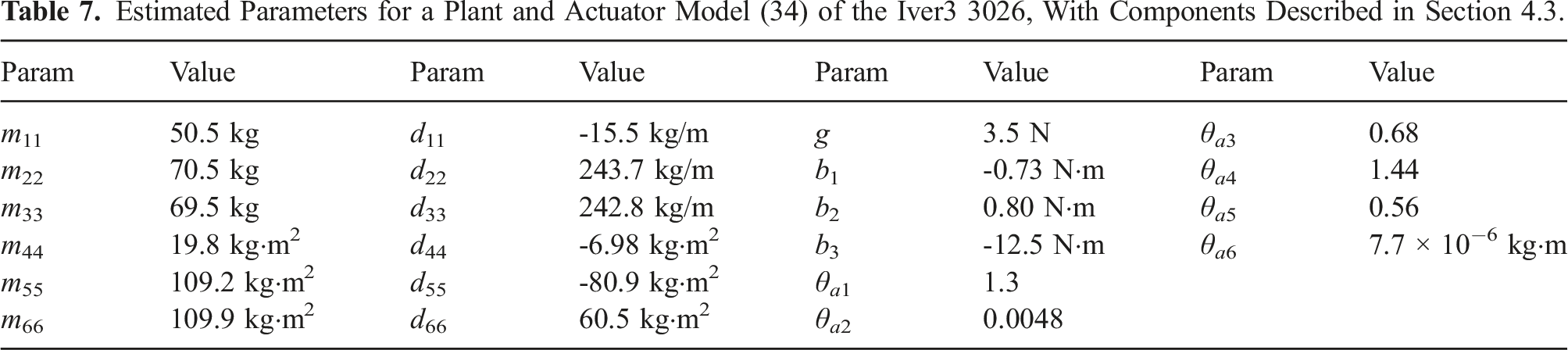
Estimated Parameters for a Plant and Actuator Model (34) of the Iver3 3026, With Components Described in Section 4.3.

Param	Value	Param	Value	Param	Value	Param	Value
m 11	50.5 kg	d 11	-15.5 kg/m	g	3.5 N	θ a3	0.68
m 22	70.5 kg	d 22	243.7 kg/m	b 1	-0.73 N⋅m	θ a4	1.44
m 33	69.5 kg	d 33	242.8 kg/m	b 2	0.80 N⋅m	θ a5	0.56
m 44	19.8 kg⋅m2	d 44	-6.98 kg⋅m2	b 3	-12.5 N⋅m	θ a6	7.7 × 10−6 kg⋅m
m 55	109.2 kg⋅m2	d 55	-80.9 kg⋅m2	θ a1	1.3
m 66	109.9 kg⋅m2	d 66	60.5 kg⋅m2	θ a2	0.0048

7.4. Discussion

The results presented here in Table 6 and Figure 4 show that the ability of a forward simulation of the plant model to match experimentally observed plant performance depends highly on the model parameter values, a well-known fact that has been reported previously, for example in Harris et al. (2018); McFarland and Whitcomb (2021).

In Section 6, we showed that the adaptively identified parameters converge to the true parameters from an arbitrary initialization in a simulation study (in which the simulated “true” parameters are known) when the PE condition (134) is satisfied. However, we cannot compare the experimentally identified parameters to the true model parameters for two reasons:

(1) We do not know the true Iver3 AUV model parameters a priori.

(2) As observed in Section 4.5, the “true” parameters are not unique, but may be any element of the set P(θ) (37).

Thus, the experimental validity of this AID algorithm can be evaluated only by the ability of the estimated parameters to predict the UV’s velocity in forward simulation. As proven in Section 4.5.2, any parameter vector in the set P(θ) (37) will result in identical vehicle model input-output dynamics.

The results reported in Figure 4 show that the experimentally identified model (Table 7) performs far better than the model using the arbitrarily chosen initial parameter set (Table 5). Further, these results show that the identified parameter set performs approximately as well on the validation data as it does on the training data. We note that the angular-velocity data obtained by the more accurate KVH sensor were not used in the training of the AID and were used only to provide as close to a source of “ground truth” as is available for angular velocity.

We observed that the performance of the identified model is worst in sway and roll DOF. We believe this phenomenon is caused by the lack of precisely controlled excitation in these DOF.

8. Conclusion

This paper reports the theory and experimental evaluation of a novel adaptive identification (AID) algorithm for the simultaneous estimation of plant-model parameters and actuator parameters for underactuated vehicles in six degrees-of-freedom (DOF).

The simulation and experimental results reported herein indicate that it is feasible to use the AID algorithm for parameter estimation of underactuated underwater vehicles (UVs) in 6-DOF. Underactuated UVs are by far the most common class of UVs, but parameter estimation is more difficult for underactuated UVs than for fully actuated UVs because the reduced actuation necessarily reduces the plant excitation that can be induced from the control inputs. Additionally, underactuated UVs are often controlled with hydrodynamic control surfaces which are difficult to characterize.

The theoretical results reported herein provide the first reported AID algorithm with proof of convergence of the parameter estimates to the true set of parameters for this class of vehicles when a persistence of excitation condition is satisfied. Most previously reported AID approaches for this class of systems only show stability and boundedness of the parameter estimates.

The simulation and experimental results show that parameters estimated using this AID can converge with a “single training set” containing on the order of 1000 s of free-motion AUV dive data. The performance of the resulting model was verified in both self-validation and cross-validation. Additionally, this AID algorithm does not require access to body linear and angular acceleration signals, which can offer an advantage over other parameter-estimation methods.