Online and offline learning of player objectives from partial observations in dynamic games

Abstract

Robots deployed to the real world must be able to interact with other agents in their environment. Dynamic game theory provides a powerful mathematical framework for modeling scenarios in which agents have individual objectives and interactions evolve over time. However, a key limitation of such techniques is that they require a priori knowledge of all players’ objectives. In this work, we address this issue by proposing a novel method for learning players’ objectives in continuous dynamic games from noise-corrupted, partial state observations. Our approach learns objectives by coupling the estimation of unknown cost parameters of each player with inference of unobserved states and inputs through Nash equilibrium constraints. By coupling past state estimates with future state predictions, our approach is amenable to simultaneous online learning and prediction in receding horizon fashion. We demonstrate our method in several simulated traffic scenarios in which we recover players’ preferences, for, e.g. desired travel speed and collision-avoidance behavior. Results show that our method reliably estimates game-theoretic models from noise-corrupted data that closely matches ground-truth objectives, consistently outperforming state-of-the-art approaches.

1. Introduction

To operate safely and efficiently in environments shared with other agents, robots must be able to predict the effects of their actions on the decisions of others. In many such settings, agents do not form a single team that shares a joint objective. Instead, each agent may have an individual objective, encoded by a cost function which they optimize unilaterally. Unless the objectives of all agents are perfectly aligned, agents must therefore compete to minimize their own cost, while accounting for the strategic behavior of others. For example, consider the highway navigation scenario in Figure 1. Here, each driver travels along the highway with an individual objective that encodes their preferences for speed, acceleration, and proximity to other cars. In heavy traffic, the objectives of drivers may conflict. For instance, if car 1 (blue) wishes to maintain its speed, it must overtake the slower vehicles in front. At the same time, however, the faster car 2 (orange) may wish maintain its speed and but would be forced to decelerate if the driver of car 1 changes lanes.

Figure 1.

5-player highway driving scenario, modeled as a dynamic game. Solving the “forward” problem amounts to finding optimal trajectories (right) for all cars, given their objectives (left). In contrast, this paper addresses the “inverse,” that is, it estimates the objectives of each player given noise-corrupted observations of each agent’s trajectories. For example, our method can infer properties such as the degree to which each player wishes to keep a safe distance from others (heat map, left). These learned objectives constitute an abstract model which can be used to predict players’ actions in the future.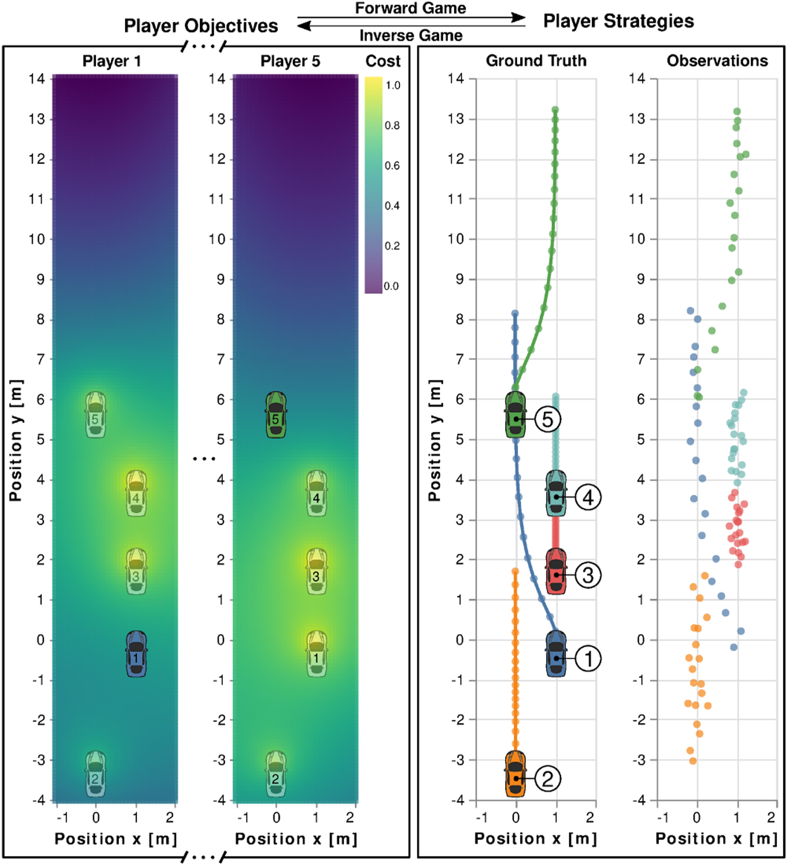

Mathematically, such interactions of multiple agents with individual, potentially conflicting objectives are characterized by a noncooperative dynamic game. The theory underpinning dynamic games is well established (Isaacs 1954-1955; Başar and Olsder 1999), and recent work has put forth efficient algorithms to determine equilibrium solutions to these problems, given players’ objectives (Fridovich-Keil et al., 2020; Di and Lamperski 2019). The forward game problem is depicted in Figure 1 (left to right) for the highway driving scenario: given the cost functions of all players (left), a forward game solver computes their rational strategies and corresponding future trajectories (right).

Unfortunately, the objectives of agents in a scene are often not known a priori. Therefore, in order for game-theoretic methods to find practical application in fields such as robotics, it is imperative to recover these objectives from data. This inverse dynamic game problem is illustrated in Figure 1 (right to left) for the highway driving scenario: given observations of player’s strategies (right), an inverse game solver recovers objectives (left) which explain the observed behavior. This inverse dynamic game problem is the focus of this work.

The challenge of recovering objectives from observed behavior has been extensively studied in the literature on inverse optimal control (IOC) (Kalman 1964; Mombaur et al., 2010; Albrecht et al., 2011) and inverse reinforcement learning (IRL) (Ng and Russell 2000; Ziebart et al., 2008). Unfortunately, however, these methods are fundamentally limited to the single-player setting. While recent efforts extend these ideas to multi-agent IRL (Šošić et al., 2016; Natarajan et al., 2010), those approaches are limited to games with potential cost structures (Monderer and Shapley 1996) and do not directly apply in general noncooperative settings. While initial work extends IOC methods to address this limitation (Rothfuß et al., 2017; Inga et al., 2019; Awasthi and Lamperski 2020), these inverse dynamic game solvers rely upon full observation of states and inputs of all players.

The main contribution of this work is a novel method for learning player’s objectives in noncooperative dynamic games from only noise-corrupted, partial state observations. In addition to learning a cost model for all players, our method also recovers a forward game solution consistent with the learned objectives by enforcing equilibrium constraints on latent trajectory estimates. This bilevel formulation further allows to couple observed and predicted behavior to recover player’s objectives even from temporally incomplete interactions. As a result, our approach is amenable for online learning and prediction in receding horizon fashion.

This paper builds upon and extends our earlier work (Peters et al., 2021). In this work, we provide a more in-depth analysis of that approach. Additionally, while our original work was limited to offline operation and could therefore only recover players’ objectives for interactions which had already occurred, in this work we remove this requirement.

We evaluate our method in extensive Monte Carlo simulations in several traffic scenarios with varying numbers of players and interaction geometries. Empirical results show that our approach is more robust to partial state observations, measurement noise, and unobserved time-steps than existing methods, and consequently it is more suitable for predicting agents’ actions in the future.

2. Prior work

We begin by discussing recent advances in the well-studied area of IOC. While methods from that field address only single-player, cooperative settings, this body of work exposes many of the important mathematical and algorithmic concepts that appear in games. We discuss how some of these approaches have been applied in the noncooperative multi-player setting and emphasize the connections between existing approaches and our contributions.

2.1. Single-player inverse optimal control

The IOC problem has been extensively studied since the well-known work of Kalman (1964). In the context of IRL, early formulations such as that of Ng and Russell (2000) and maximum-entropy variants (Ziebart et al., 2008; Kretzschmar et al., 2016) have proven successful in treating problems with discrete state and control sets. In robotic applications, optimal control problems typically involve decision variables in a continuous domain. Hence, recent work in IOC differs from the IRL literature mentioned above as it is explicitly designed for smooth problems.

One common framework for addressing IOC problems with nonlinear dynamics and nonquadratic cost structures is bilevel optimization (Mombaur et al., 2010; Albrecht et al., 2011). Here, the outer problem is a least squares or maximum likelihood estimation (MLE) problem in which demonstrations are matched with a nominal trajectory estimate and decision variables parameterize the objective of the underlying optimal control problem. The inner problem determines the nominal trajectory estimate as the optimizer of the “forward” (i.e., standard) optimal control problem for the outer problem’s decision variables. A key benefit of bilevel IOC formulations is that they naturally adapt to settings with noise-corrupted partial state observations (Albrecht et al., 2011).

Early bilevel formulations for IOC utilize derivative-free optimization schemes to estimate the unknown objective parameters in order to avoid explicit differentiation of the solution to the inner optimal control problem (Mombaur et al., 2010). That is, the inner solver is treated as a black-box mapping from cost parameters to optimal trajectories which is utilized by the outer solver to identify the unknown parameters using a suitable derivative-free method. While black-box approaches can be simple to implement due to their modularity and lack of reliance on derivative information, they often suffer from a high sampling complexity (Nocedal and Wright 2006). Since each sample in the context of black-box IOC methods amounts to solving a full optimal control problem, such approaches remain intractable for scenarios with large state spaces or additional unknown parameters, such as unknown initial conditions.

Other works instead embed the Karush–Kuhn–Tucker (KKT) conditions of the inner problem as constraints on the outer problem. Since these techniques enforce only first-order necessary conditions of optimality, globally optimal observations are unnecessary and locally optimal demonstrations suffice. Yet, a key computational difficulty of KKT-constrained IOC formulations is that they yield a nonconvex optimization problem due to decision variables in the outer problem appearing nonlinearly with inner problem variables in KKT constraints. This occurs even in the relatively benign case of linear-quadratic IOC.

In contrast to bilevel optimization formulations where necessary conditions of optimality are embedded as constraints, recent methods (Levine and Koltun 2012; Englert and Toussaint 2018; Awasthi 2019; Menner and Zeilinger 2020; Jin et al., 2021) minimize the residual of these conditions directly at the demonstrations. Since the observed demonstration is assumed to satisfy any constraints of the underlying forward optimal control problem, this method can be formulated as fully unconstrained optimization. Additionally, these residual formulations yield a convex optimization problem if the class of objective functions is convex in the unknown parameters at the demonstration (Keshavarz et al., 2011; Englert and Toussaint 2018). This condition holds in the common setting of linearly parameterized objective functions. Levine and Koltun (2012) propose a variant of this approach that utilizes quadratic approximations of the reward model around demonstrations to derive optimality residuals in a maximum entropy framework. Englert and Toussaint (2018) present extensions of this method do accommodate inequality constraints on states and inputs. Much like KKT-constrained formulations, these residual methods operate on locally optimal demonstrations. However, an important limitation of residual methods is that they require observations of full state and input sequences. More recently, Menner and Zeilinger (2020) compared IOC techniques based on KKT constraints and residuals and demonstrated inferior performance of the latter even in problems with linear dynamics and quadratic target objectives.

Our work takes inspiration from the KKT-constraint formulation for single-player IOC as discussed by Albrecht et al. (2011) and Menner and Zeilinger (2020). While these works apply only to single-player settings, we utilize the necessary conditions for open-loop Nash equilibriums (OLNEs) (Başar and Olsder 1999) to generalize this approach to noncooperative multi-player scenarios.

2.2. Multi-player inverse dynamic games

Many of the IOC techniques discussed above have close analogues in the context of multi-player inverse dynamic games.

As in single-player IOC, methods akin to black-box bilinear optimization have also been studied in the context of inverse games (Peters 2020; Le Cleac’h et al., 2021). Peters (2020) uses a particle-filtering technique for online estimation of human behavior parameters. This work demonstrates the importance of inferring human behavior parameters for accurate prediction in interactive scenarios. However, there, inference is limited to a single parameter and the work highlights the challenges associated with scaling this sampling-based approach to high-dimensional latent parameter spaces. Le Cleac’h et al. (2021) employ a similar derivative-free filtering technique based on an unscented Kalman filter. While this approach drastically reduces the overall sample complexity, it still relies on exact observations of the state to reduce the required number of solutions to full dynamic games at the inner level.

Another line of research has put forth solution techniques for inverse games that follow from the residual methods outlined in Section 2.1 (Köpf et al., 2017; Rothfuß et al., 2017; Awasthi and Lamperski 2020; Inga et al., 2019). Köpf et al. (2017) study a special case of an inverse linear-quadratic game in which the equilibrium feedback strategies of all but one player are known. This assumption reduces the estimation problem to single-player IOC to which the residual methods discussed above can be applied directly. Rothfuß et al. (2017) present a more general approach that does not exploit such special structure but instead minimizes the residual of the first-order necessary conditions for a local OLNE. Inga et al. (2019) present a variant of this OLNE residual method in a maximum entropy framework, generalizing the single-player IOC algorithm proposed by Levine and Koltun (2012). Recently, Awasthi and Lamperski (2020) also extended the OLNE residual method of Rothfuß et al. (2017) to inverse games with state and input constraints. This approach extends that of Englert and Toussaint (2018) to noncooperative multi-player scenarios.

All of these inverse game KKT residual methods share many properties with their single-player counterparts. In particular, since they rely upon only local equilibrium criteria, they are able to recover player objectives even from local-rather than only global-equilibrium demonstrations. However, as in the single-player case, they rely upon observation of both state and input to evaluate the residuals.

In contrast to KKT residual methods (Rothfuß et al., 2017; Awasthi and Lamperski 2020; Inga et al., 2019), we enforce these conditions as constraints on a jointly estimated trajectory, rather than minimizing the residual of these conditions directly at the observation. By maintaining a trajectory estimate in this manner, our method explicitly accounts for observation noise, partial state observability, and unobserved control inputs. Furthermore, in contrast to black-box approaches to the inverse dynamic game problem (Peters 2020; Le Cleac’h et al., 2021), our method does not require repeated solutions of the underlying forward game. Moreover, our method returns a full forward game solution in addition to the estimated objective parameters for all players.

3. Background: Open-loop Nash games

While this work is concerned with the inverse game problem of learning objectives from observed behavior, we first provide a technical introduction to the theory of forward open-loop dynamic Nash games. These forward games correspond to the model that we seek to recover in this work. Furthermore, as we shall discuss in Section 4, they may be used at the inner level of a bilevel optimization problem to formulate the inverse game problem.

As discussed in Section 1, dynamic games provide an expressive mathematical formalism for modeling the strategic interactions of multiple agents with differing objectives. Interested readers are directed to Başar and Olsder (1999) for a more complete discussion. We note that dynamic games afford a wide variety of equilibrium concepts; our choice of open-loop Nash equilibria in this work captures scenarios in which players do not account for future information gains and instead commit to a sequence of control decisions a priori. These conditions may occur when occlusions prevent future information gains or when bounded rationality causes players to ignore them. OLNEs have been demonstrated to capture dynamic interaction when embedded in receding-horizon re-planning schemes (Wang et al., 2019; Le Cleac’h et al., 2020). Beyond that, restricting our attention to OLNEs engenders computational advantages which are discussed below. Other choices of solution concept are possible and should be explored in future work. Recent methods such as those of Di and Lamperski (2019) and Le Cleac’h et al. (2020) facilitate efficient solutions to the “forward” open-loop games given players’ objectives a priori.

3.1. Preliminaries

Consider a game played between N players over discrete time-steps t ∈ [T]≔{1, …, T}. The game is composed of three key components: dynamics, objectives (which are later presumed to be unknown in this work), and information structure.

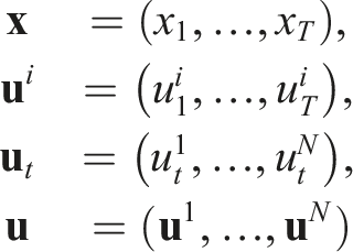
We presume that the game is Markov with respect to state $x\in {\mathbb{R}}^n$ . That is, given each player’s control input $u^i\in {\mathbb{R}}^{m^i},i\in \left[N\right]$ , the state evolves according to the difference equation

$x_{t+1}=f_t\left(x_t,u_t^1,\dots ,u_t^N\right)$

(1)

For clarity, we shall introduce the following shorthand notation

$\begin{array}{cc}\mathbf{x}& =\left(x_1,\dots ,x_T\right),\\ {\mathbf{u}}^i& =\left(u_1^i,\dots ,u_T^i\right),\\ {\mathbf{u}}_t& =\left(u_t^1,\dots ,u_t^N\right),\\ \mathbf{u}& =\left({\mathbf{u}}^1,\dots ,{\mathbf{u}}^N\right)\end{array}$

Observe that the state x pertains to the entire game, not only to a single player. In the examples presented in this paper, x is simply the concatenation of individual players’ states, and correspondingly the dynamics are independent for all players. However, this is not always the case, and the methods developed here apply in the more general settings as well.

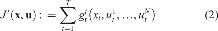
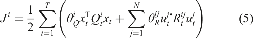
The objective of player i is encoded by their distinct cost function J ⁱ , which they seek to minimize. This cost can in general depend upon the sequence of states and inputs for all players. ¹ In this paper, we presume that objectives are expressed in time-additive form, as is common across the optimal control and reinforcement learning literature

$J^i\left(\mathbf{x},\mathbf{u}\right):={\displaystyle \sum }_{t=1}^T{g}_t^i\left(x_t,u_t^1,\dots ,u_t^N\right)$

(2)

Since the state trajectory x follows equation (1), these cost functions can also be written in terms of the initial condition x₁ and the sequence of control inputs for all players u. For this reason, we shall also use the notation J ⁱ (u; x₁) and refer to the tuple of initial state, dynamics, and objectives as follows

$\mathrm{\Gamma }:=\left(x_1,{\left\{f_t\right\}}_{t\in \left[T\right]},{\left\{J^i\right\}}_{i\in \left[N\right]}\right)$

(3)

Finally, the information structure of a dynamic game refers to the information available to each player when they are required to make a decision at each time. At time t, then, Player-i’s input is a function ${\gamma }_t^i:{\mathcal{I}}_t^i\to {\mathbb{R}}^{m^i}$ , where ${\mathcal{I}}_t^i$ is the set of information available to Player-i at time t. In this paper, we consider open-loop information structures, that is, where ${\mathcal{I}}_t^i=\left\{x_1\right\}$ . ² In open-loop information, then, it suffices for Player-i to specify their input sequence u ⁱ given a fixed initial condition x₁. For this reason, we neglect a more detailed treatment of strategy spaces and information structure and simply refer to the finite-dimensional sequence of control inputs for each player.

This characterization of a dynamic game is intentionally general. Our solution methods will rely upon established numerical methods for smooth optimization, however, and as such we require the following assumption.

Assumption 1

(Smoothness) Dynamics f and objectives J ⁱ have well-defined second derivatives in all state and control variables, at all times and for all players.

Most physical systems of interest and interactions thereof are naturally modeled in this way. However, we note that, for example, hybrid dynamics such as those induced by contact do not satisfy this assumption.

We shall illustrate key concepts using a consistent “running example” throughout the paper.

Running example

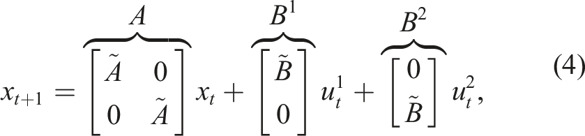
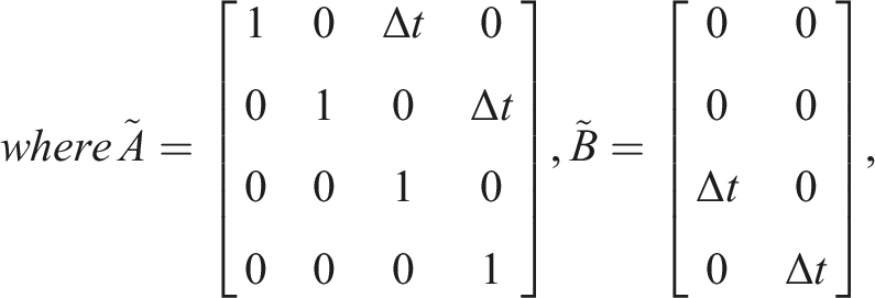
Consider an N = 2-player linear-quadratic (LQ) game that is, one in which dynamics f _t are linear in state x _t and control inputs u _t , and costs J ⁱ are quadratic in states and controls. Let each player independently follow the dynamics of a double integrator in the Cartesian plane. State $x=\left(p_x^1,p_y^1,{\dot{p}}_x^1,{\dot{p}}_y^1,p_x^2,p_y^2,{\dot{p}}_x^2,{\dot{p}}_y^2\right)$ then evolves with inputs $u^i=\left({\ddot{p}}_x^i,{\ddot{p}}_y^i\right)$ according to

$\begin{array}{c}{x}_{t+1}=\stackrel{A}{\overbrace{\left[\begin{array}{cc}\stackrel{\sim }{A}& 0\\ 0& \stackrel{\sim }{A}\end{array}\right]}}{x}_t+\stackrel{B^1}{\overbrace{\left[\begin{array}{c}\stackrel{\sim }{B}\\ 0\end{array}\right]}}{u}_t^1+\stackrel{B^2}{\overbrace{\left[\begin{array}{c}0\\ \stackrel{\sim }{B}\end{array}\right]}}{u}_t^2,\end{array}$

(4)

$\begin{array}{cc}& where\hspace{0.17em}\stackrel{\sim }{A}=\left[\begin{array}{cccc}1& 0& \mathrm{\Delta }t& 0\\ 0& 1& 0& \mathrm{\Delta }t\\ 0& 0& 1& 0\\ 0& 0& 0& 1\end{array}\right],\stackrel{\sim }{B}=\left[\begin{array}{cc}0& 0\\ 0& 0\\ \mathrm{\Delta }t& 0\\ 0& \mathrm{\Delta }t\end{array}\right],\end{array}$

and Δt is a uniform time discretization, for example., 0.1s. Each player has a quadratic objective of the form

$J^i=\frac{1}{2}{\displaystyle \sum }_{t=1}^T\left({\theta }_Q^i{x}_t^{\mathrm{T}}{Q}_t^i{x}_t+{\displaystyle \sum }_{j=1}^N{\theta }_R^{ij}{u}_t^{j•}{R}_t^{ij}{u}_t^j\right)$

(5)

In this simple example, $Q_t^i$ and $R_t^{ij}$ are known, positive definite matrices encoding the preferences of each player. The scalars ${\theta }_Q^i\in \mathbb{R}$ and ${\theta }_R^{ij}\in \mathbb{R}$ weight these known matrices. In this paper, we develop a technique to learn a priori unknown parameters such as the costs weights above from both offline and online data. Note that this simple LQ game shall only serve to explain the general concepts of our method. For our experiments presented in Section 7 , we consider more complex problems with nonlinear dynamics and nonquadratic costs, such as the 5-player highway navigation problem shown in Figure 1 .

3.2. The Nash solution concept

Combining these components, each player i in an open-loop dynamic game seeks to solve the following optimization problem

$\forall i\in \left[N\right]\{\begin{array}{ll}\underset{\mathit{x},{\mathbf{u}}^i}{\min } J^i\left(\mathbf{u};x_1\right)& \left(6\mathrm{a}\right)\\ \mathrm{s}.\mathrm{t}. {\mathit{x}}_{t+1}=f_t\left({\mathit{x}}_t,{\mathbf{u}}_t\right),\forall t\in \left[T-1\right].& \left(6\mathrm{b}\right)\end{array}$

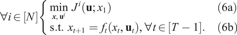
There exist a variety of distinct solution concepts for such smooth open-loop dynamic games. In this paper, we consider the well-known Nash equilibrium concept, wherein no player has a unilateral incentive to change its strategy. Mathematically, the Nash concept is defined as follows.

Definition 1

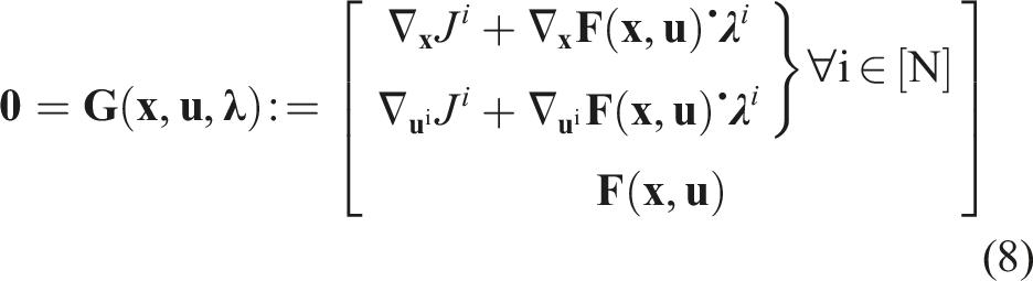
(Open-loop Nash equilibrium) The strategies u*≔(u¹*, …, u^N∗) constitute an open-loop Nash equilibrium (OLNE) in the game $\mathrm{\Gamma }=\left(x_1,{\left\{f_t\right\}}_{t\in \left[T\right]},{\left\{J^i\right\}}_{i\in \left[N\right]}\right)$ if the following inequalities hold:

$J^{i*}=J^i\left({\mathbf{u}}^{*};x_1\right)\le J^i\left(\left({\mathbf{u}}^i,{\mathbf{u}}^{-i*}\right);x_1\right),\forall i\in \left[N\right]$

(7)

Here, we use the shorthand (u ⁱ , u ⁻ⁱ *) to indicate the collection of strategies in which only Player-i deviates from the Nash profile, that is, u ⁱ ≠ u ⁱ *.

Note that, at a Nash equilibrium, each player must independently have no incentive to deviate from its strategy. Since players’ objectives may generally conflict, the Nash concept encodes noncooperative, rational, and potentially selfish behavior.

Unfortunately, Nash equilibria are known to be very difficult to find in general (Daskalakis et al., 2009). In this work, we seek only local equilibria which satisfy the Nash conditions equation (7) to first order. That is, following similar approaches in both single-player IOC (Albrecht et al., 2011; Englert and Toussaint 2018) and forward/inverse open-loop games (Le Cleac’h et al., 2020; Awasthi 2019), we encode forward optimality via the corresponding first-order necessary conditions. These first-order necessary conditions are given by the union of the individual players’ KKT conditions, that is

$\begin{array}{l}\mathbf{0}=\mathbf{G}\left(\mathbf{x},\mathbf{u},\mathbf{\lambda }\right):=\left[\begin{array}{c}\begin{array}{c}{\nabla }_{\mathbf{x}}{\mathit{J}}^{\mathit{i}}+{\nabla }_{\mathbf{x}}\mathbf{F}{\left(\mathbf{x},\mathbf{u}\right)}^{•}{\mathit{\lambda }}^{\mathit{i}}\\ {\nabla }_{{\mathbf{u}}^{\mathrm{i}}}{\mathit{J}}^{\mathit{i}}+{\nabla }_{{\mathbf{u}}^{\mathrm{i}}}\mathbf{F}{\left(\mathbf{x},\mathbf{u}\right)}^{•}{\mathit{\lambda }}^{\mathit{i}}\end{array}\}\forall \mathrm{i}\in \left[\mathrm{N}\right]\\ \mathbf{F}\left(\mathbf{x},\mathbf{u}\right)\end{array}\right]\end{array}$

(8)

Here, the first two block rows are repeated for all players, and the function F (x, u) accumulates the dynamic constraints of equation (6a) at all time steps, with the t^th row given by ${\mathit{x}}_{\mathit{t}+1}-{\mathit{f}}_{\mathit{t}}\left({\mathit{x}}_{\mathit{t}},{\mathit{u}}_{\mathit{t}}^1,\dots ,{\mathit{u}}_{\mathit{t}}^N\right)$ . Note that we have also introduced costate variables ${\mathit{\lambda }}^{\mathit{i}}:=\left({\mathit{\lambda }}_1^{\mathit{i}},\dots ,{\mathit{\lambda }}_{\mathit{T}-1}^{\mathit{i}}\right)$ for each player, with ${\mathit{\lambda }}_{\mathit{t}}^{\mathit{i}}\in {\mathbb{R}}^n$ the Lagrange multiplier corresponding to Player-i’s dynamics constraint in equation (6a) at time step t. Note that, as with control inputs, we use the notation λ ≔( λ ¹, …, λ ^N ).

Running example

Consider the two-player LQ example above with double integrator dynamics given by equation (4) and quadratic objectives given by equation (5). The t ^th block of the first row of equation (8) is given by

$\mathbf{0}={\theta }_Q^i{Q}_t^i{x}_t+{\lambda }_{t-1}^i-A^{•}{\lambda }_t^i$

(9)

for Player-i. Likewise, the t ^th block of the second row of equation (8) for Player-i is given by

$\mathbf{0}={\theta }_R^{ii}{R}_t^{ii}{u}_t^i-B^{i•}{\lambda }_t^i$

(10)

Finally, the t ^th block of the final row of equation (8) is given by

$\mathbf{0}=x_{t+1}-A{x}_t-B^1{u}_t^1-B^2{u}_t^2$

(11)

Computationally, the KKT conditions of the forward game, given in equation (8), are a set of, generally nonlinear, equality constraints in the variables x, u, and λ . To find a solution, that is, a root of G (x, u, λ ), we may employ a root-finding algorithm such as a variant of Newton’s method (Nocedal and Wright 2006: Chapter 11). This is the approach taken by, for example, Le Cleac’h et al. (2020).

Running example

For our LQ example, it can be seen that a single step of Newton’s method on G (⋅) amounts to the well-known Riccati solution to an open-loop LQ game ( Başar and Olsder 1999 : Chapter 6. ³

4. Problem setup

Solving a forward Nash game amounts to identifying optimal strategies for all players, provided a priori knowledge of their objectives Jⁱ. By contrast, in this work we are concerned with the inverse Nash problem, that is, that of identifying players’ objectives which explain their observed behavior. To develop the inverse Nash problem, here we shall presume that learning occurs offline, given a sequence of noisy, partial observations of all players’ state. The method we develop for this setting, however, is amenable to trajectory prediction and online, receding horizon operation as discussed in Section 5.2.

We formulate the inverse Nash problem as one of offline learning, in which players’ objectives belong to a known parametric function class. To that end, we make the following assumption.

Assumption 2

(Parametric objectives) Player-i’s cost function is fully described by a vector of parameters ${\theta }^i\in {\mathbb{R}}^{k^i}$ . That is, $J^i\left(·;{\theta }^i\right)\equiv {\sum }_{t=1}^T{g}_t^i\left(x_t,u_t^1,\dots ,u_t^N;{\theta }^i\right)$ .

Recalling Assumption 1, the functions ${\mathit{g}}_{\mathit{t}}^{\mathit{i}}\left(·;{\mathit{\theta }}^{\mathit{i}}\right)$ have well-defined derivatives in states x_t and controls uⁱ. We shall also extend this smoothness assumption to include the parameters themselves.

Assumption 3

(Smoothness in parameter space) Extending Assumption 1, we require that stage cost functions $g_t^i\left(·;{\theta }^i\right)$ have well-defined first- and second-derivatives with respect to the parameter vector θ ⁱ .

This smoothness assumption is quite general. For example, players’ stage costs ${\mathit{g}}_{\mathit{t}}^{\mathit{i}}\left(·;{\mathit{\theta }}^{\mathit{i}}\right)$ may be encoded as arbitrary function approximators such as artificial neural networks. In this work, we choose a more interpretable (though less flexible) parametric structure; we defer an investigation of more general cost structures for future work. In particular, the examples considered here use a linearly parameterized structure in which ${\mathit{g}}_{\mathit{t}}^{\mathit{i}}\left(·;{\mathit{\theta }}^{\mathit{i}}\right)$ is a linear function of θⁱ, that is, ${\mathit{g}}_{\mathit{t}}^{\mathit{i}}\left(·; {\mathit{\theta }}^{\mathit{i}}\right)\equiv {\mathit{\theta }}^{\mathit{i}T}{\stackrel{\sim }{\mathit{g}}}_{\mathrm{t}}^{\mathit{i}}(·)$ for some set of potentially nonlinear basis functions ${\stackrel{\sim }{\mathit{g}}}_{\mathrm{t}}^{\mathit{i}}(·)$ . By incorporating appropriate domain-specific knowledge, however, these relatively simple cost structures are able to encapsulate complex, strategic interactions such as the highway lane changes of Figure 1.

Running example

Recall the quadratic objectives of equation ( 5 ), and take cost parameters ${\theta }^i={\left({\theta }_Q^i,{\theta }_R^{ij}\right)}_{j\in \left[N\right]}$ . Observe, therefore, that Player-i’s objective depends linearly upon its cost parameters θ ⁱ .

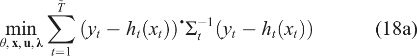
Thus equipped, the objective learning problem reduces to maximizing the likelihood of a sequence of partial state observations y ≔(y₁,…,y_T) for the parametric class of games $\mathrm{\Gamma }\left(\mathit{\theta }\right)=\left({\mathit{x}}_{\mathit{1}},f,{\left\{J^{\left(\mathit{i}\right)}\left(·;{\mathit{\theta }}^{\left(\mathit{i}\right)}\right)\right\}}_{\mathit{i}\mathit{\in }\left[\mathit{N}\right]}\right)$ . Formally, we seek to solve a problem of the form

$\begin{array}{cc}\underset{\theta ,\mathit{x},\mathbf{u}}{\max }& p\left(\mathbf{y}\mid \mathbf{x},\mathbf{u}\right)\end{array}$

(12a)

$\begin{array}{cc}\mathrm{s}.\mathrm{t}.& \left(\mathbf{x},\mathbf{u}\right)\hspace{0.17em}\mathrm{i}\mathrm{s}\hspace{0.17em}\mathrm{a}\mathrm{n}\hspace{0.17em}\mathrm{O}\mathrm{L}\mathrm{N}\mathrm{E}\hspace{0.17em}\mathrm{o}\mathrm{f}\mathrm{\Gamma }\left(\theta \right)\end{array}$

(12b)

$\begin{array}{cc}& \left(\mathbf{x},\mathbf{u}\right)\hspace{0.17em}\mathrm{i}\mathrm{s}\hspace{0.17em}\mathrm{d}\mathrm{y}\mathrm{n}\mathrm{a}\mathrm{m}\mathrm{i}\mathrm{c}\mathrm{a}\mathrm{l}\mathrm{l}\mathrm{y}\hspace{0.17em}\mathrm{f}\mathrm{e}\mathrm{a}\mathrm{s}\mathrm{i}\mathrm{b}\mathrm{l}\mathrm{e}\hspace{0.17em}\mathrm{u}\mathrm{n}\mathrm{d}\mathrm{e}\mathrm{r}\hspace{0.17em}f\end{array},$

(12c)

where θ aggregates all players’ cost parameters, that is, θ≔(θ¹,…,θ ^N ), and p(y∣x, u) constitutes a known observation likelihood, or measurement, model.

Remark 1

(Initial state) Observe that x ₁ is an explicit decision variable in equation ( 12a ), whereas it represents a constant (known) initial condition in the forward game problem discussed in Section 3 . This reflects the fact that the state trajectory, including initial conditions, must be estimated as part of the inverse problem. As we shall see, estimating the state trajectory jointly with the cost parameters allows our method to be less sensitive to observation noise.

This measurement model is arbitrary, though, following Assumption 1 and Assumption 3, it must be smooth. In the simplest instance, we may receive an exact measurement of the sequence of states and inputs for all players. In that case, the measurement model p(y∣x, u) reduces to a Dirac delta function. More generally, p(y∣x, u) may be an arbitrary smooth probability density function, making our formulation amenable to realistic sensors such as cameras or LiDARs.

Prior work in both single-player IOC, such as that of Englert and Toussaint (2018), and inverse games, such as those of Awasthi and Lamperski (2020) and Rothfuß et al. (2017), presumes a degenerate measurement model in which states and controls are observed directly without any noise. When perfect observations are unavailable, these methods naturally extend by first estimating a sequence of likely states and controls (a standard nonlinear filtering problem). In Section 6, we describe these sequential estimation methods in greater detail. In contrast, our formulation given in equation (12b) encodes a coupled estimation problem in which states, control inputs, and cost parameters must all be estimated simultaneously. Thus, our method exploits the additional coupling imposed by the Nash equilibrium constraints onto the unknowns. In Section 7, we conduct a series of Monte Carlo experiments to quantify the advantages afforded by simultaneous learning over sequential estimation.

5. Equilibrium-constrained cost learning

Here we present our core contribution, a mathematical formulation of objective inference in multi-agent, noncooperative games. We express this problem as a nonconvex optimization problem with equilibrium constraints, which we relax into a standard-format equality-constrained nonlinear program.

5.1. Offline learning

We first consider the problem of learning each player’s objective from previously recorded data of prior interactions, offline.

Equation (12c) is a mathematical program with equilibrium constraints (Luo et al., 1996; Ferris et al., 2005), with the nested equilibrium conditions of equation (12b) encoding the Nash inequalities of Definition 1. Equilibrium constraints generalize bilevel programming, and computational approaches tend to be less mature than those for standard-form (in)equality-constrained programming.

We relax the equilibrium constraint of equation (12b) by replacing it with its KKT conditions, that is, by substituting equation (8). This yields the following equation

$\begin{array}{cc}\underset{\theta ,\mathbf{x},\mathbf{u},\mathbf{\lambda }}{\max }& p\left(\mathbf{y}\mid \mathbf{x},\mathbf{u}\right)\end{array}$

(13a)

$\begin{array}{cc}\mathrm{s}.\mathrm{t}.& \mathbf{G}\left(\mathbf{x},\mathbf{u},\mathbf{\lambda };\theta \right)\end{array}=0$

(13b)

Here, we have explicitly written the KKT conditions from equation (8) in terms of the cost parameters θ. Additionally, observe that in equation (13a), the costates λ required to evaluate the KKT conditions G (⋅; θ) appear as additional primal variables. The constraints of equation (subsection 13b) will be assigned their own Lagrange multipliers, which are distinct from the original costates. By letting states, control inputs, and costates be primal variables, the KKT conditions G (⋅) do not depend explicitly upon the observations y. Thus, solving equation (13b) does not require complete state or input observations; rather, the equilibrium constraints of equation (subsection 13b) allow us to reconstruct this missing information while we estimate cost parameters θ, simultaneously. Several remarks are in order.

Remark 2

(Multiple observed trajectories) We have developed equation ( 13a ) for the setting in which a single trajectory ( x , u ) has been observed, yielding a measurement sequence y . However, our approach affords straightforward extension to settings in which player’s objectives are learned from multiple demonstrations. In this instance, the primal variables ( x , u , λ ) would be replicated for all trajectories, although the cost parameters θ would be shared. The objective given by equation ( 13a ) would be replaced by the joint probability of all measurements conditioned on all underlying trajectories, and the equilibrium constraints in equation ( 13b ) would be concatenated for all trajectories.

Remark 3

(Regularizing parameters) Depending upon the parametric structure of players’ objectives J ⁱ (⋅; θ ⁱ ), and hence the structure of KKT residual G (⋅; θ), it can be critical to regularize and/or constrain cost parameters. For example, if there exists a choice of θ ⁱ for Player-i such that J ⁱ ( x , u ; θ ⁱ ) is constant for all dynamically feasible trajectories ( x , u ), then every such trajectory would satisfy the equilibrium constraint of equation ( 12b ). Such choices of θ must be avoided, for example, by regularizing or otherwise constraining parameters.

Running example

Following Remark 3, we constrain the parameters θ ⁱ ≥ c > 0. Moreover, to account for scale invariance, we constrain their sum to unity, that is, ${\sum }_{i\in \left[N\right]}\left({\theta }_Q^i+{\sum }_{j\in \left[N\right]}{\theta }_R^{ij}\right)=1$ .

5.1.1. Least squares

A common observation model p(y∣x, u) is the additive white Gaussian noise (AWGN) model. Here, each observation y_t depends only upon the current state x_t and control inputs u _t , that is

$y_t=h_t\left(x_t,{\mathbf{u}}_t\right)+n_t$

(14)

where the (potentially nonlinear) function h_t computes the expected measurement and n_t is a zero-mean Gaussian white noise process with known covariance, that is, ${\mathit{n}}_{\mathit{t}}\sim \mathcal{N}\left(0,{\mathrm{\Sigma }}_{\mathit{t}}\right)$ . In this case, following standard methods in maximum likelihood estimation (Gallager 2013), it is straightforward to express the maximization in equation (13a) as nonlinear least squares by taking the negative logarithm of p(y∣x, u)

$\underset{\theta ,\mathbf{x},\mathbf{u},\mathbf{\lambda }}{\min }{\displaystyle \sum }_{t=1}^T{\left(y_t-h_t\left(x_t\right)\right)}^{•}{\mathrm{\Sigma }}_t^{-1}\left(y_t-h_t\left(x_t\right)\right)$

(15a)

$\begin{array}{cc}\mathrm{s}.\mathrm{t}.& \mathbf{G}\left(\mathbf{x},\mathbf{u},\mathbf{\lambda };\theta \right)=\mathbf{0}\end{array}$

(15b)

in summary, this inverse problem entails the following task: Find those parameters θ for which the corresponding game solution generates expected observations near the observed data. This formulation of the inverse game problem can be encoded using well-established numerical modeling languages such as CasADi (Andersson et al., 2019) or JuMP (Dunning et al., 2017), and solved using off-the-shelf optimization routines such as IPOPT (Wächter and Biegler 2006) or SNOPT (Gill et al., 2005).

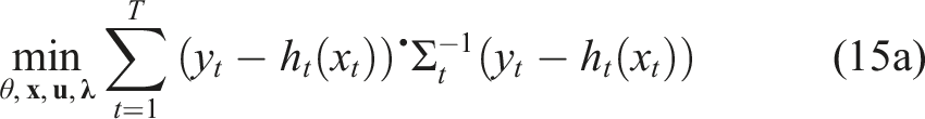
5.1.2. Problem complexity

Let us examine the structure of the least squares problem in equation (15a) more carefully. In general, the observation map h_t (⋅) and KKT conditions G(⋅; ⋅) may be arbitrarily nonlinear. Therefore, without further structural assumptions, our formulation is an equality-constrained nonlinear least squares problem. Due primarily to the nonlinearities in G, equation (15b) is generally nonconvex. Solution methods, therefore, may be sensitive to initial values of primal variables; we discuss a straightforward initialization scheme in Section 6.1.

Perhaps surprisingly, this nonconvexity persists in the LQ setting of our running example, even when h_t (⋅) is the identity.

Running example

Consider the LQ setting, with ${\theta }^i={\left({\theta }_Q^i,{\theta }_R^{ij}\right)}_{j\in \left[N\right]}$ as before. Let the observation map be the identity, that is, h _t (x _t ) = x _t and presume AWGN. The resulting nonlinear least squares problem in equation ( 15a ) has constraints of the form given in equations ( 9 ) to ( 11 ). Let us consider the first of these constraints for a single time step t and Player-i

$\mathbf{0}={\theta }_Q^i{Q}_t^i{x}_t+{\lambda }_{t-1}^i-A^{•}{\lambda }_t^i$

Recall that the decision variables in our formulation are (θ, x, u, λ ). Here, we see that θⁱ multiplies x_t. At best, therefore, this constraint is a bilinear equality, making the overall problem in equation (15b) nonconvex even for this minimal inverse LQ game.

When we directly observe both state and control inputs without noise, that is, y_t ≡ (x_t, u _t ), these constraints become linear even in the general non-LQ setting, so long as players’ objectives are linearly parameterized. In this setting, we may rewrite equation (9) as follows

$\begin{array}{cc}\mathbf{0}& ={\nabla }_{x_t}\stackrel{{\theta }^{i\top }{\stackrel{\sim }{g}}_t^i(·)}{\overbrace{g_t^i\left(x_t,u_t;{\theta }^i\right)}}+{\lambda }_{t-1}^i-{\nabla }_{x_t}{f}_t{\left(x_t,u_t\right)}^{•}{\lambda }_t^i\end{array}$

(16a)

$\begin{array}{cc}& ={\theta }^{iT}{\nabla }_{x_t}{\stackrel{\sim }{g}}_t^i\left(x_t,u_t\right)+{\lambda }_{t-1}^i-{\nabla }_{x_t}{f}_t{\left(x_t,u_t\right)}^{•}{\lambda }_t^i\end{array}$

(16b)

with this observation model, then, the only decision variables are $\left({\mathit{\theta }}^{\mathit{i}},{\mathit{\lambda }}_{\mathit{t}}^{\mathit{i}},{\mathit{\lambda }}_{\mathit{t}-1}^{\mathit{i}}\right)$ , which all appear linearly. Furthermore, the least squares objective in equation (15a) becomes unnecessary, since, by assumption, the measurements y already include the states x exactly. Incorporating these simplifications, the entire constrained least squares problem of equation (15a) reduces to the problem

$\begin{array}{cc}\mathrm{f}\mathrm{i}\mathrm{n}\mathrm{d}& \theta ,\mathbf{\lambda }\end{array}$

(17a)

$\begin{array}{cc}\mathrm{s}.\mathrm{t}.& \mathbf{0}={\theta }^{i\top }{\nabla }_{x_t}{\stackrel{\sim }{g}}_t^i\left(x_t,u_t\right)+{\lambda }_{t-1}^i\\ & -{\nabla }_{x_t}{f}_t{\left(x_t,u_t\right)}^{•}{\lambda }_t^i,\forall i,t\end{array}$

(17b)

$\begin{array}{cc}& \mathbf{0}={\theta }^{i\top }{\nabla }_{u_t^i}{\stackrel{\sim }{g}}_t^i\left(x_t,u_t\right)\\ & -{\nabla }_{u_t^i}{f}_t{\left(x_t,u_t\right)}^{•}{\lambda }_t^i,\forall i,t\end{array}$

(17c)

Because the constraints in equation (17a) are linear, the problem is equivalent to a linear system of equations. Moreover, since the constraints are completely decoupled for each player, they may be solved separately and in parallel for all players to obtain cost parameters θ ⁱ and costates λ ⁱ . This reduction forms the basis for the state of the art in solving inverse dynamic games (Rothfuß et al., 2017; Awasthi and Lamperski 2020), which only apply in settings with perfect state and input observations. To compare against these methods in more general settings that feature noise, unobserved inputs, and partial state measurements, we augment these methods with a sequential optimization procedure in Section 6. Comparative Monte Carlo studies of all approaches are presented in Section 7.

5.2. Online learning

While Section 5.1 estimates the objectives of interacting agents from recorded data offline, our formulation for inverse Nash problems extends naturally to an online learning setting; i.e. cost learning from observations of ongoing interactions. As we shall discuss below, our method can perform online cost learning and trajectory prediction simultaneously, making it suitable for receding horizon applications.

5.2.1. Learning with prediction

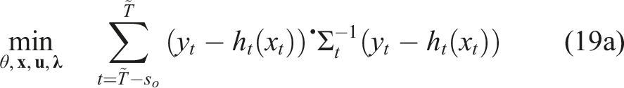
Equipped with a tractable solution strategy for the setting of offline learning, we now consider a coupled prediction and learning problem. Similar problems have been considered in the single-agent setting by, e.g. Jin et al. (2021) and Mukadam et al. (2019). Here, we aim to learn the cost parameters θ from only a subset of the game horizon; i.e., we presume that observations $\mathbf{y}=\left({\mathit{y}}_1,\dots ,{\mathit{y}}_{\stackrel{\sim }{\mathit{T}}}\right)$ where the observation horizon $\stackrel{\sim }{\mathit{T}}\le \mathit{T}$ . Despite this change, the original problem of equation (12a) remains effectively unchanged; only the objective has changed. In particular, by substituting the KKT conditions for an OLNE in place of the original equilibrium constraint as in equation (13a), and making AWGN assumptions, we recover a variant of the constrained least squares formulation of equation (15a)

$\underset{\theta ,\mathbf{x},\mathbf{u},\mathbf{\lambda }}{\min }{\displaystyle \sum }_{t=1}^{\stackrel{\sim }{T}}{\left(y_t-h_t\left(x_t\right)\right)}^{•}{\mathrm{\Sigma }}_t^{-1}\left(y_t-h_t\left(x_t\right)\right)$

(18a)

$\begin{array}{cc}\mathrm{s}.\mathrm{t}.& \mathbf{G}\left(\mathbf{x},\mathbf{u},\mathbf{\lambda };\theta \right)=\mathbf{0}\end{array}$

(18b)

Note that the upper limit of addition is $\stackrel{\sim }{\mathit{T}}$ , rather than T as in equation (15a), while the OLNE KKT conditions in equation (subsection 18b) depend upon states, inputs, and costates for all times $\mathit{t}\in \left\{1,\dots ,\stackrel{\sim }{\mathit{T}},\dots ,\mathit{T}\right\}$ .

Despite the similarities between this problem and equation (15a), the Nash trajectory (x∗, u*), which emerges as a solution, affords a new interpretation. In particular, for times $\mathit{t}\le \stackrel{\sim }{\mathit{T}}$ , these equilibrium states and controls constitute filtered estimates of the observed quantities y, while for times $\mathit{t}>\stackrel{\sim }{\mathit{T}}$ they represent predictions of the future. Importantly, however, extending trajectories beyond the observation horizon $\stackrel{\sim }{\mathit{T}}$ adds additional constraints to equation (15b). This ability to incorporate future, unobserved states makes the method more robust and data efficient when only a fraction of the game horizon is observed. Consequently, this formulation can be employed for online learning in scenarios of ongoing interactions. We provide a detailed empirical analysis of this setting in Section 7.2.2. A summary of this variant of our inverse game solver is provided in Figure 2(a).

Figure 2.

Schematic overview of inverse game solvers set up for online operation. (a) Our method computes player’s objectives, state estimates, and trajectory predictions jointly. (b) The baseline requires full knowledge of states and inputs and therefore must preprocess raw observations before it can estimate players’ objectives. In order to generate trajectory predictions, the baseline must solve an additional forward game formulated over the estimated initial states and objectives.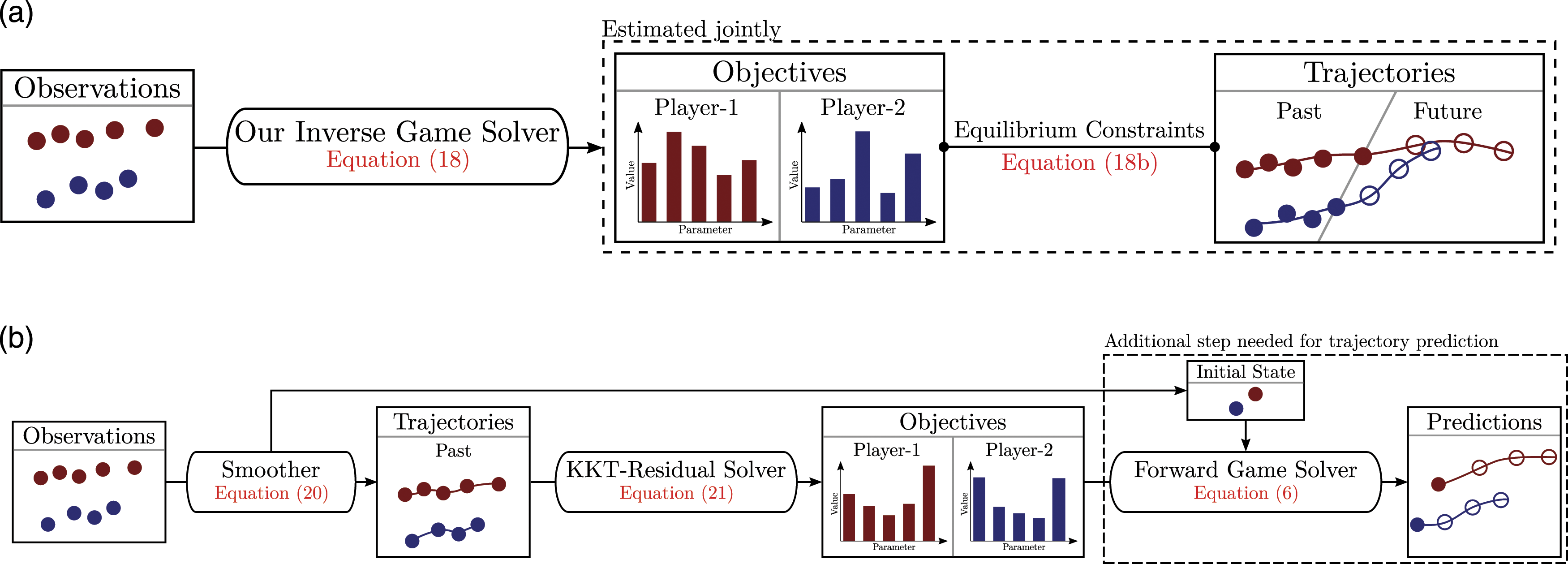

5.2.2. Receding horizon learning

Our method is directly amenable to receding horizon, online operation. Here, we suppose that the agents interact over the half-open time-interval $\mathit{t}\in \left\{1,\dots ,\stackrel{\sim }{\mathit{T}},\dots ,\infty \right\}$ , and that observations exist for $\mathit{t}\le \stackrel{\sim }{\mathit{T}}$ . Here, $\stackrel{\sim }{\mathit{T}}$ may be interpreted as the current time and, as time elapses, both $\stackrel{\sim }{\mathit{T}}$ and the overall prediction horizon T increase accordingly. Unfortunately, however, increasing the overall problem horizon increases the number of variables in equation (12a), eventually making the problem intractable.

To simplify matters, we approximate the learning problem at each instant by neglecting all times outside the interval $\left\{\stackrel{\sim }{\mathit{T}}-{\mathit{s}}_{\mathit{o}},\dots ,\stackrel{\sim }{\mathit{T}},\dots ,\stackrel{\sim }{\mathit{T}}+{\mathit{s}}_{\mathit{p}}\right\}$ , where s_o is the length of a fixed-lag buffer of past observations and s_p is the horizon of future state predictions. In this setting, the total number of variables remains constant (since the length of this interval is constant), rendering equation (12b) tractable to solve online. More precisely, at time $\stackrel{\sim }{\mathit{T}}$ (and under AWGN assumptions), we solve a modified version of equation (18b)

$\underset{\theta ,\mathbf{x},\mathbf{u},\mathbf{\lambda }}{\min }\hspace{1em}{\displaystyle \sum }_{t=\stackrel{\sim }{T}-s_o}^{\stackrel{\sim }{T}}{\left(y_t-h_t\left(x_t\right)\right)}^{•}{\mathrm{\Sigma }}_t^{-1}\left(y_t-h_t\left(x_t\right)\right)$

(19a)

$\begin{array}{cc}\mathrm{s}.\mathrm{t}.& \mathbf{G}\left(\mathbf{x},\mathbf{u},\mathbf{\lambda };\theta \right)=\mathbf{0}\end{array}$

(19b)

where the KKT constraint G (⋅) is understood to depend upon times $\mathit{t}\in \left\{\stackrel{\sim }{\mathit{T}}-{\mathit{s}}_{\mathit{o}},\dots ,\stackrel{\sim }{\mathit{T}},\dots ,\stackrel{\sim }{\mathit{T}}+{\mathit{s}}_{\mathit{p}}\right\}$ and states, control inputs, and costates are also limited to that interval. At each later time, we solve a problem with identical structure, with the understanding that $\stackrel{\sim }{\mathit{T}}$ will have changed to reflect the elapsed time. In effect, this procedure amounts to simultaneous fixed-lag smoothing and receding-horizon prediction. We simulate this online learning procedure in Section 7.3.2.

6. Baseline

Recall the discussion of Section 5.1.2, in which we show that—with noiseless observations of states x and controls u, and linear cost parameterization ${\mathit{g}}_{\mathit{t}}^{\mathit{i}}\left(·;{\mathit{\theta }}^{\mathit{i}}\right)\equiv {\mathit{\theta }}^{\mathit{i}T}{\stackrel{\sim }{\mathit{g}}}_{\mathrm{t}}^{\mathit{i}}(·)$ —our formulation reduces to the linear system of equations of equation (17a). This reduction underlies state-of-the-art methods for learning the objectives of players in games (Rothfuß et al., 2017; Awasthi and Lamperski 2020). Therefore, such methods unfortunately require noiseless observations of the full state and input sequences for all players. In contrast, our approach in equation (13b) is amenable to noisy, partial observations.

6.1. Recovering unobserved variables

To provide a meaningful comparison between our proposed technique and the state-of-the-art in settings with imperfect observations, we augment (Rothfuß et al., 2017; Awasthi and Lamperski 2020) with a pre-processing to estimate unobserved states and inputs. To that end, we solve the following relaxed version of equation (13a)

$\stackrel{\sim }{\mathbf{x}},\stackrel{\sim }{\mathbf{u}}:=\arg \underset{\mathbf{x},\mathbf{u}}{\max }\mathit{p}\left(\mathbf{y}\mid \mathbf{x},\mathbf{u}\right)$

(20a)

$\begin{array}{cc}\mathrm{s}.\mathrm{t}.& \mathbf{F}\left(\mathbf{x},\mathbf{u}\right)=\mathbf{0}\end{array}$

(20b)

As in Section 5.1.1, under an AWGN assumption equation (20a) becomes equality-constrained nonlinear least squares. However, unlike equation (15a), we have neglected the first two rows of the equilibrium constraint given in equation (8). That is, equation (20b) computes a maximum likelihood estimate of states and inputs irrespective of the underlying game structure.

The solution of this smoothing problem is used as an estimate of states and inputs when the baseline is employed in partially observed settings. Beyond that, the same procedure serves as simple, yet effective initialization scheme for our method to tackle issues of non-convexity discussed in Section 5.1.2.

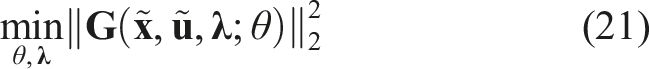
6.2. Minimizing KKT residuals

Like our proposed method, the state-of-the-art methods developed by Rothfuß et al. (2017) and Awasthi and Lamperski (2020) use the forward game’s KKT conditions to measure the quality of a set of cost parameters θ. While we compare to this derivative-based, KKT condition approach, we note that other approaches outlined in Section 2.2 such as Le Cleac’h et al. (2021) utilize black-box optimization methods and do not require or exploit derivative information. These significant algorithmic differences and the resulting differences in sample complexity, locality of solutions, etc., make a direct comparison difficult to interpret.

Specifically, the KKT residual method of Awasthi and Lamperski (2020) and Rothfuß et al. (2017) fixes the state and input sequences to their observed—or in our case, estimated via equation (20a)—values. Fixing these variables, however, the resulting linearly constrained satisfiability problem of equation (17c) may be infeasible, depending upon the parametric structure of costs ${\mathit{g}}_{\mathit{t}}^{\mathit{i}}\left(·;{\mathit{\theta }}^{\mathit{i}}\right)$ . In lieu, state-of-the-art approaches minimize the KKT residual itself, that is

$\underset{\theta ,\mathbf{\lambda }}{\min }{\Vert \mathbf{G}\left(\stackrel{\sim }{\mathbf{x}},\stackrel{\sim }{\mathbf{u}},\mathbf{\lambda };\theta \right)\Vert }_2^2$

(21)

In prior work (Awasthi and Lamperski 2020; Rothfuß et al., 2017), $\stackrel{\sim }{\mathbf{x}}$ and $\stackrel{\sim }{\mathbf{u}}$ are assumed to be directly observed. As discussed in Section 6.1, here we presume they are the results of the pre-processing step given in equation (20a). Additionally, like the linear system of equations in equation (17a), the only decision variables here are the objective parameters θ and the costates λ . In effect, the baseline does not refine the state and input estimates given by the pre-processing step of equation (20b). Furthermore, as in equation (17b), the problem may be decomposed into separate problems for each player and solved in parallel. In essence, then, this KKT residual formulation neglects the coupling between players’ actions which is encoded in the equilibrium conditions; computationally, it reduces to solving separate IOC problems for each player neglecting game-theoretic interactions with others.

A schematic overview of this baseline approach is depicted in Figure 2. By first estimating the states x and inputs u from measurements y, and only afterward learning the cost parameters θ and associated costates λ , the KKT residual method can be thought of as a sequential decomposition of our approach. By contrast, our formulation maintains (x, u) as decision variables and refines the initial guess of $\left(\stackrel{\sim }{\mathbf{x}},\stackrel{\sim }{\mathbf{u}}\right)$ by identifying all variables simultaneously.

7. Experiments

In this work, we develop a technique for learning players’ objectives in continuous dynamic games from noise-corrupted, partial state observations. We conduct a series of Monte Carlo studies to examine the relative performance of our proposed methods and the KKT residual baseline in both offline and online learning settings. ⁴

7.1. Experimental setup

We implement our proposed approach as well as the KKT residual baseline of Rothfuß et al. (2017) in the Julia programming language (Bezanson et al., 2017), using the mathematical modeling framework JuMP (Dunning et al., 2017). As a consequence, our implementation encodes an abstract description of equation (13b), making it straightforward to use in concert with a variety of optimization routines. In this work, we use the open source COIN-OR IPOPT algorithm (Wächter and Biegler 2006). The source code for our implementation is publicly available. ⁵

To evaluate the relative performance of our proposed approach with the KKT residual baseline, we perform several Monte Carlo studies. The details of these studies are described below. However, all of these studies share the following overall setup: we fix a cost parameterization for each player, find corresponding OLNE trajectories as roots of equation (8) using the well-known iterated best response (IBR) algorithm (Wang et al., 2019), and simulate noisy observations thereof with additive white Gaussian noise (AWGN) as in equation (14). Each study then presents samples across a different problem parameter to test the sensitivity of both approaches to observation noise (Sections 7.2.1 and 7.3.1) and unobserved time-steps (Section 7.2.2) in two different problem settings.

In each of the studies below, we consider N vehicles navigating traffic, and instantiate game dynamics and player objectives as follows. Each vehicle has its own state x ⁱ such that the global game state is concatenated as x = (x¹, …, x ^N ). Further, each vehicle follows unicycle dynamics at time discretization Δt

$x_{t+1}^i=\{\begin{array}{ll}\left(x-\mathit{position}\right)\hspace{0.17em}{p}_{x,t+1}^i& =p_{x,t}^i+\mathrm{\Delta }t\hspace{0.17em}{v}_t^i\mathit{cos}{\psi }_t^i\\ \left(y-\mathit{position}\right)\hspace{0.17em}{p}_{y,t+1}^i& =p_{y,t}^i+\mathrm{\Delta }t\hspace{0.17em}{v}_t^i\mathit{sin}{\psi }_t^i\\ \left(\mathit{heading}\right)\hspace{0.17em}{\psi }_{t+1}^i& ={\psi }_t^i+\mathrm{\Delta }t\hspace{0.17em}{\omega }_t^i\\ \left(speed\right)\hspace{0.17em}{v}_{t+1}^i& =v_t^i+\mathrm{\Delta }t\hspace{0.17em}{a}_t^i,\end{array}$

(22)

where ${\mathit{u}}_{\mathit{t}}^{\mathit{i}}=\left({\omega }_t,a_t\right)$ includes the yaw rate and longitudinal acceleration. Finally, each player’s objective is characterized by a stage cost ${\mathit{g}}_{\mathit{t}}^{\mathit{i}}$ which is a weighted sum of several basis functions, that is

$g_t^i={\displaystyle \sum }_{\mathcal{\ell }=1}^5{w}_{\mathcal{\ell }}^i{g}_{\mathcal{\ell },t}^i\{\begin{array}{ll}{g}_{1,t}^i=\mathbf{1}\hspace{0.17em}\left(t\ge T-t_{\text{goal}}\right)d\left(x_t^i,x_{\text{goal}}^i\right)& \left(23\mathrm{a}\right)\\ g_{2,t}^i=-{\displaystyle \sum }_{j\ne i}\mathit{log}\left({\Vert p_i-p_j\Vert }_2^2\right)& \left(23\mathrm{b}\right)\\ g_{3,t}^i={\left(v^i\right)}^2& \left(23\mathrm{c}\right)\\ g_{4,t}^i={\left({\omega }_t^i\right)}^2& \left(23\mathrm{d}\right)\\ g_{5,t}^i={\left(a_t^i\right)}^2.& \left(23\mathrm{e}\right)\end{array}$

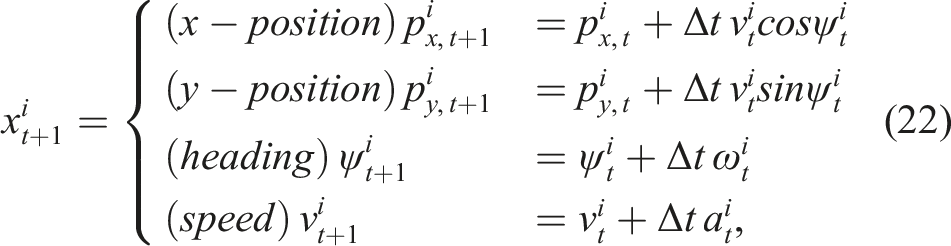
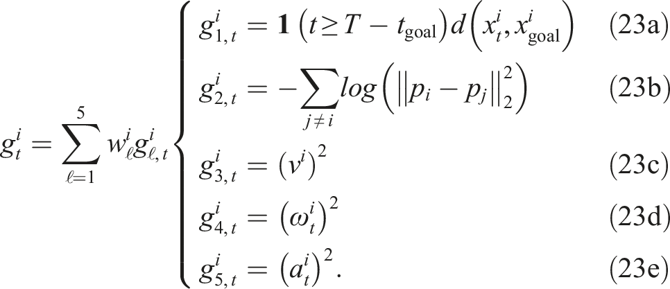
Here, the cost parameters ${\mathit{\theta }}^{\mathit{i}}={\left(w_{\mathcal{\ell }}^{\mathit{i}}\right)}_{\mathcal{\ell }\in \left[5\right]},w_{\mathcal{\ell }}^{\mathit{i}}\in {\mathbb{R}}_{+}$ are positive weights for each cost component. Further, $p_i=\left(p_x^{\mathit{i}},p_y^{\mathit{i}}\right)$ denotes the planar position of Player-i, and d (⋅, ⋅) is an arbitrary distance mapping. For example, we may choose $\mathrm{d}\left(x_t^{\mathit{i}},x_{\mathrm{goal}}^{\mathit{i}}\right)=\Vert p_t^{\mathit{i}}-p_{\mathrm{goal}}^{\mathit{i}}{\Vert }_2^2$ to compute squared distance from a fixed goal position. Note, however, that this map is generic and can also be used to encode more complex goal-reaching specifications as in the highway lane-changing example depicted in Figure 1. Taken together, the basis functions encode the following aspects of each player’s preferences:

1. Be close to the goal state within the last t_goal time steps (23a).

2. Avoid close proximity to other vehicles (23b).

3. Avoid high speeds (23c).

4. Avoid large control efforts (23d, 23e).

Games of this form are inherently noncooperative since players must compete to reach their own goals efficiently while avoiding collision with one another. Hence, they must negotiate these conflicting objectives and thereby find an equilibrium of the underlying game.

In all of the Monte Carlo studies, we evaluate the approaches for two different noisy observation models ${\mathit{h}}_t^{\mathrm{full}}$ and ${\mathit{h}}_t^{\mathrm{partial}}$ . In ${\mathit{h}}_t^{\mathrm{full}}\left({\mathit{x}}_{\mathit{t}}\right):={\mathit{x}}_{\mathit{t}}$ , estimators observe the full state, and in ${\mathit{h}}_t^{\mathrm{partial}}\left({\mathit{x}}_{\mathit{t}}\right):=\left({\mathit{p}}_t^{\mathrm{1}},{\mathrm{\psi }}_t^{\mathrm{1}},\dots ,{\mathit{p}}_t^{\mathit{N}},{\mathrm{\psi }}_t^{\mathit{N}}\right)$ , estimators observe the position and heading but not the speed of each agent, that is, they receive a partial state observation.

7.2. Detailed analysis of a 2-player game

We first study the performance of our method in a simplified, N = 2-player game. This set of experiments demonstrates the performance gap of our approach and the KKT residual baseline in methods in a conceptually simple and easily interpretable scenario. Here, the game dynamics are given as in equation (22), and player objectives are parameterized as in equation (23a). In particular, we let $\mathrm{d}\left(x_t^{\mathit{i}},x_{\mathit{goal}}^{\mathit{i}}\right)=\Vert p_t^{\mathit{i}}-p_{\mathit{goal}}^{\mathit{i}}{\Vert }_2^2$ . In summary, therefore, each vehicle wishes to reach a fixed, known goal position in the plane while avoiding collision with the other.

7.2.1. Offline learning

We begin by studying both our method’s and the baseline’s ability to infer the unknown objective parameters θ, as developed in Section 5.1. To do so, we conduct a Monte Carlo study for the aforementioned 2-player collision-avoidance application.

We generate 40 random observation sequences at each of 22 different levels of isotropic observation noise. For each of the resulting 880 observation sequences, we run both our method and the baseline to recover estimates of weights ${\mathit{\theta }}^{\mathit{i}}={\left(w_{\mathcal{\ell }}^{\mathit{i}}\right)}_{\mathcal{\ell }\in \left[5\right]}$ for each player. Note that in this offline setting both methods learn these objective parameters from noisy observations of a single, complete game trajectory. That is, each estimate relies upon 25 s of simulated interaction history from a single scenario.

Figure 3 shows the estimator performance for varying levels of observation noise in two different metrics. Figure 3(a) reports the mean cosine error of the objective parameter estimates. That is, we measure cosine-dissimilarity between the unobserved true model parameters θ_true and the learned estimates θ_est according to

$D_{\mathit{cos}}\left({\theta }_{\text{true}},{\theta }_{\text{est}}\right)=1-\frac{1}{N}{\displaystyle \sum }_{i\in \left[N\right]}\frac{{\theta }_{\text{true}}^{i\top }{\theta }_{\text{est}}^i}{{\Vert {\theta }_{\text{true}}^i\Vert }_2{\Vert {\theta }_{\text{est}}^i\Vert }_2}$

(24)

where the mean is taken over the N players. The normalization of the parameter vectors in equation (24) reflects the fact that the absolute scaling of each player’s objective parameters does not affect their optimal behavior, holding other players’ parameters fixed. In sum, this metric measures the estimator performance in objective parameter space.

Figure 3.

Estimation performance of our method and the baseline for the 2-player collision-avoidance example, with noisy full and partial state observations. (a) Error measured directly in parameter space using equation (24). (b) Error measured in position space using equation (25). Triangular data markers in (b) highlight objective estimates which lead to ill-conditioned games. Solid lines and ribbons indicate the median and IQR of the error for each case.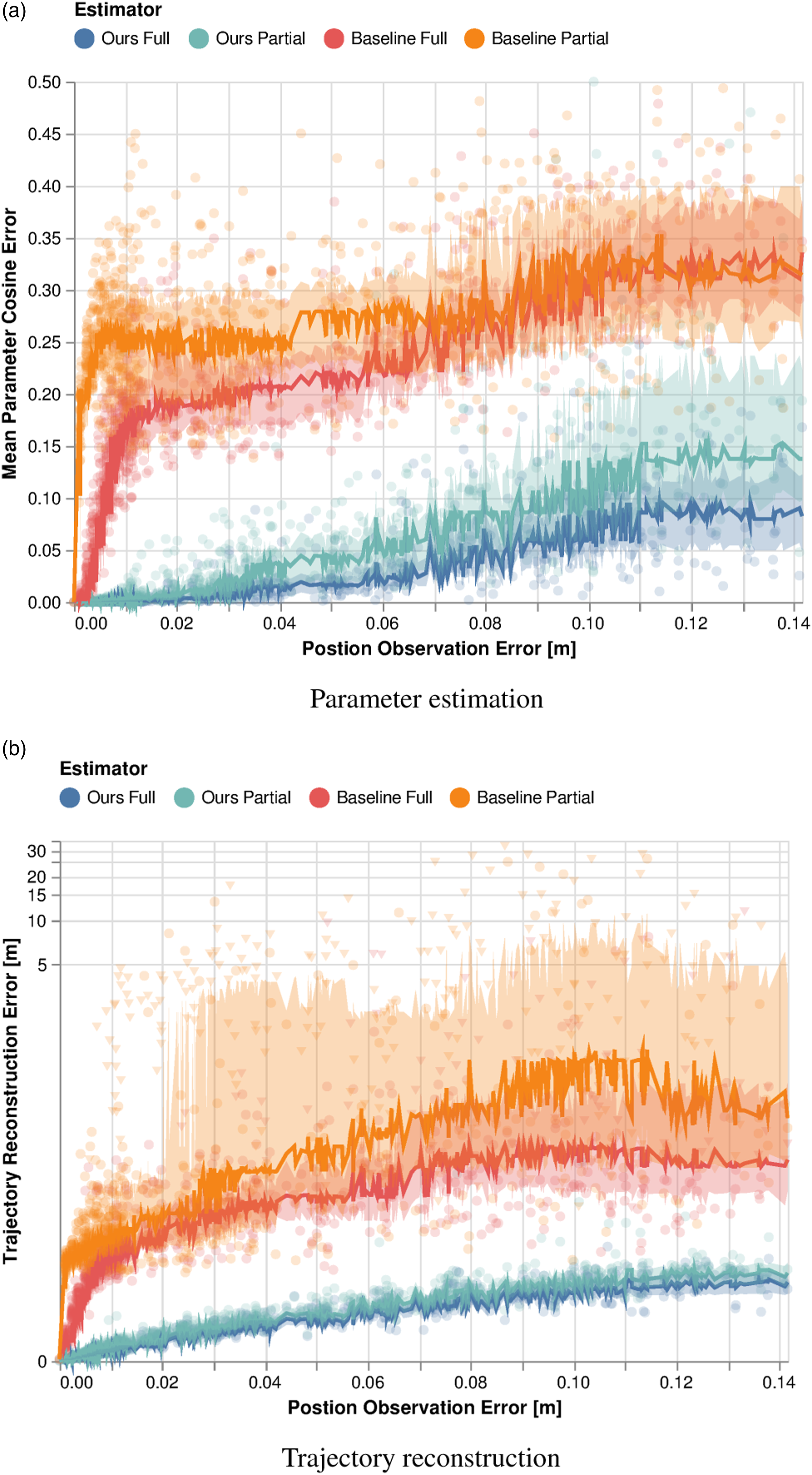

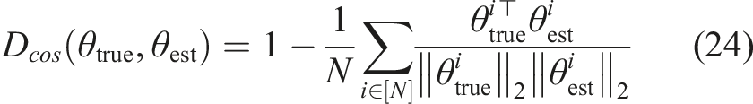
Figure 3(b) shows the mean absolute position error for trajectory reconstructions computed by finding a root of equation (8) using the estimated objective parameters. Reconstruction error allows us to inspect the quality of learned cost parameters for explaining observed vehicle motion, providing a more tangible metric of algorithmic quality. In addition to the raw data, we highlight the median as well as the interquartile range (IQR) of the estimation error over a rolling window of 60 data points.

Figure 3(a) shows that both our method and the baseline recover the true parameters θ reliably even for partial observations, if the observations are noiseless. However, the performance of the baseline degrades rapidly with increasing noise variance. This pattern is particularly pronounced in the setting of partial observations. On the other hand, our estimator recovers the unknown cost parameters more accurately in both settings, and with a smaller variance than the baseline. Thus, compared to the KKT residual baseline, the performance of our method degrades gracefully when both full and partial observations are corrupted by noise.

Next, we study these methods’ relative performance as measured by reconstruction error, as shown in Figure 3(b). Here, reconstruction error is measured according to

$D_{\text{rec}}\left({\theta }_{\text{true}},{\theta }_{\text{est}}\right)=\frac{1}{NT}{\displaystyle \sum }_{i\in \left[N\right]}{\displaystyle \sum }_{t\in \left[T\right]}{\Vert p_{\text{rec},t}^i-p_{\text{true},t}^i\Vert }_2$

(25)

where $p_{\text{true},t}^{\mathit{i}}$ denotes the true position of Player-i at time step t and $p_{\text{rec},t}^{\mathit{i}}$ denotes the position reconstructed from a Nash solution to the game with estimated cost parameters θ_est. We see similar patterns here as in the parameter error space, indicating the reliability of our method in both noisy full and partial observation settings.

Additionally, note that we have denoted some data points for the baseline method with triangular markers. For these Monte Carlo samples, the learned parameters θ_est specify ill-conditioned objectives that prevent us from recovering roots of equation (8)—essentially rendering the parameter estimates useless for downstream applications. This can happen, for example, when proximity costs dominate control input costs. For the baseline, a total of 104 out of 880 estimates result in an ill-conditioned forward game when states are fully observed. In the case of partial observations, the number of learning failures increases to 218. In contrast, our method recovers well-conditioned player objectives for all demonstrations and allows for accurate reconstruction of the game trajectory.

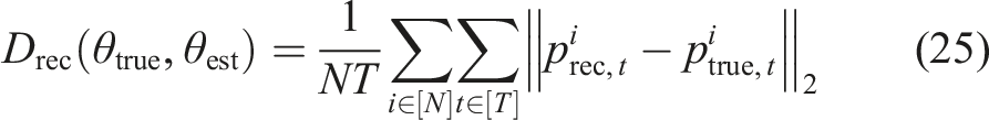
For additional intuition of the performance gap, Figure 4 visualizes the reconstruction results in trajectory space for a fixed initial condition. Figure 4(a) shows the noise corrupted demonstrations generated for isotropic AWGN with standard deviation σ = 0.1. Figures 4(b) and (c) show the corresponding trajectories reconstructed by solving the game using the objective parameters learned by our method and the baseline, respectively. Note that our method generates a far smaller fraction of outliers than the baseline. Furthermore, the performance of our method is only marginally affected by partial state observability, whereas baseline performance degrades substantially.

Figure 4.

Qualitative reconstruction performance for the 2-player collision-avoidance example at noise level σ = 0.1 for 40 different observation sequences. (a) Ground truth trajectory and observations, where each player wishes to reach a goal location opposite their initial position. (b, c) Trajectories recovered by solving the game at the estimated parameters for our method and the baseline using noisy full and partial state observations.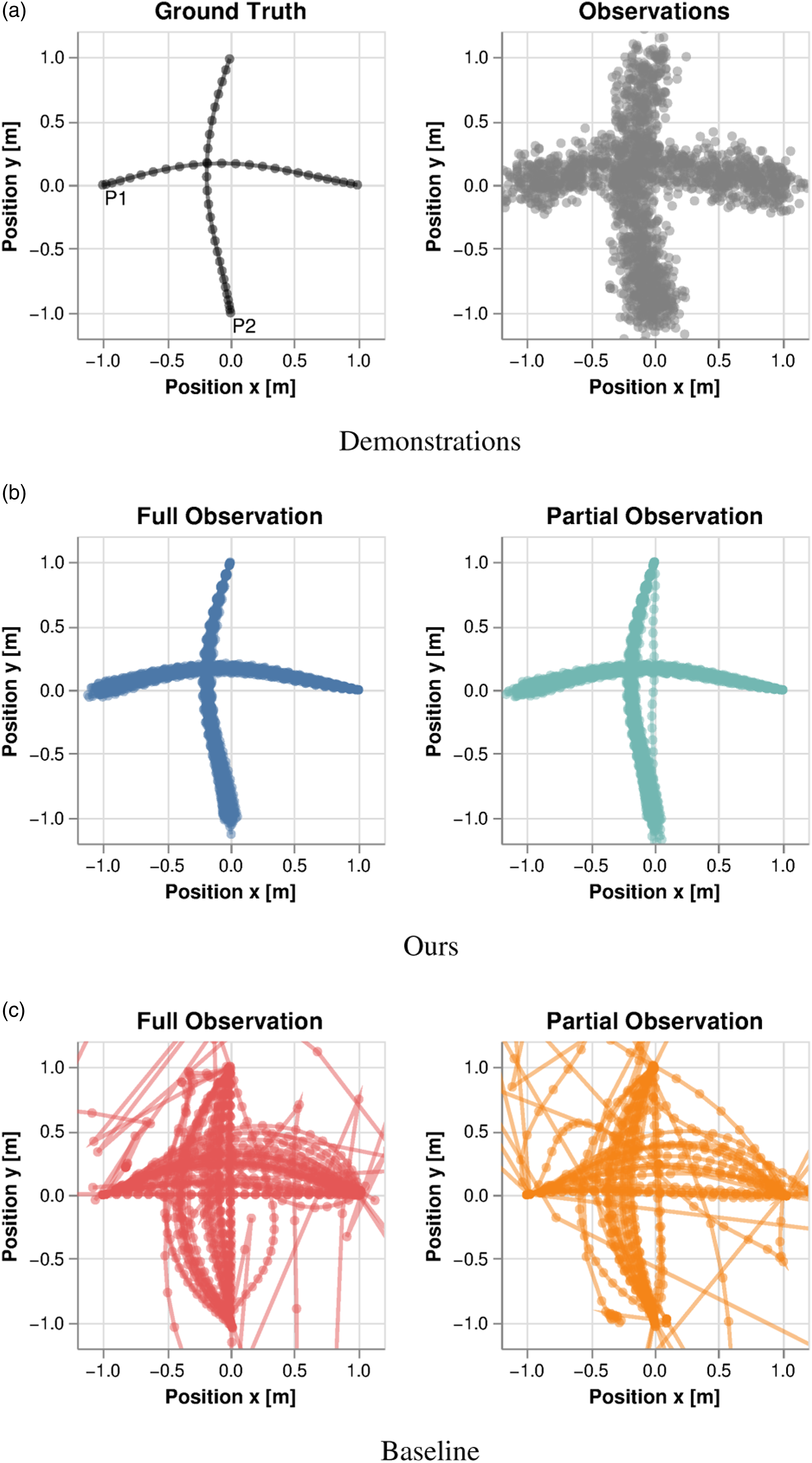

7.2.2. Online learning with prediction

Next, we study the performance of both our proposed method and the KKT residual baseline in the setting of objective learning with prediction. Following the problem description of Section 5.2.1, here, only the beginning of an unfolding dynamic game is observed. This problem naturally describes a single time frame of online operations where observations accumulate as time evolves.

We conduct a Monte Carlo analysis of the two-player collision-avoidance game from Section 7.1 in which we vary the number of observed time steps of a fixed-length game. For this truncated observation sequence, each method is tasked to learn the players’ underlying cost parameters θⁱ and predict their motion for the next s_p = 10 time steps. Our method accomplishes these coupled tasks jointly by solving equation (18b). The KKT residual baseline, however, operates on the estimates provided the preceding smoothing step, therefore, cannot couple unobserved, future time steps with cost inference. Instead, it achieves this task in a two-stage procedure: First, parameter estimates are recovered from a truncated game over only the observed $\stackrel{\sim }{\mathit{T}}$ time steps. With these parameters in hand, the baseline then predicts future game states by re-solving a forward game starting from the final state estimate ${\stackrel{\sim }{\mathrm{x}}}_{\stackrel{\sim }{\mathit{T}}}$ with time steps simulated from $t\in \left\{\stackrel{\sim }{\mathit{T}},\dots ,\stackrel{\sim }{\mathit{T}}+10\right\}$ .

In Figure 5, we vary the observation horizon $\stackrel{\sim }{\mathit{T}}\in \left\{5,\dots ,15\right\}$ for a ground-truth game played over 25 time steps. For each value of $\stackrel{\sim }{\mathit{T}}$ , we sample 40 sequences of observations ${\left\{y_t\right\}}_{t=\mathit{1}}^{\stackrel{\sim }{\mathit{T}}}$ . Here, we fix an isotropic Gaussian noise level of σ = 0.05 and measure the performance of both our method and the baseline using two distinct metrics. In Figure 5(a), we measure learning performance in parameter space using the metric given in equation (24). As shown, our approach consistently estimates the cost parameters more accurately than the baseline. Furthermore, as the observation horizon $\stackrel{\sim }{\mathit{T}}$ increases, both methods improve. In Figure 5(b), we see that these patterns persist when we measure performance in trajectory space, applying the metric of equation (25) to the predicted states ${\mathit{x}}_{\mathit{t}},t\in \left\{\stackrel{\sim }{\mathit{T}},\dots ,\stackrel{\sim }{\mathit{T}}+10\right\}$ . Indeed, in this case, the performance gap is even more pronounced. By observing only $\stackrel{\sim }{\mathit{T}}=5$ steps, our method reliably outperforms the baseline even when the baseline is given triple the number of observations.

Figure 5.

Estimation performance for our method and the baseline for varying numbers of observations of the 2-player collision-avoidance example at a fixed noise level of σ = 0.05. (a) Estimation performance measured directly in parameter space using equation (24). (b) Prediction error over the next 10 s beyond the observation horizon using equation (25).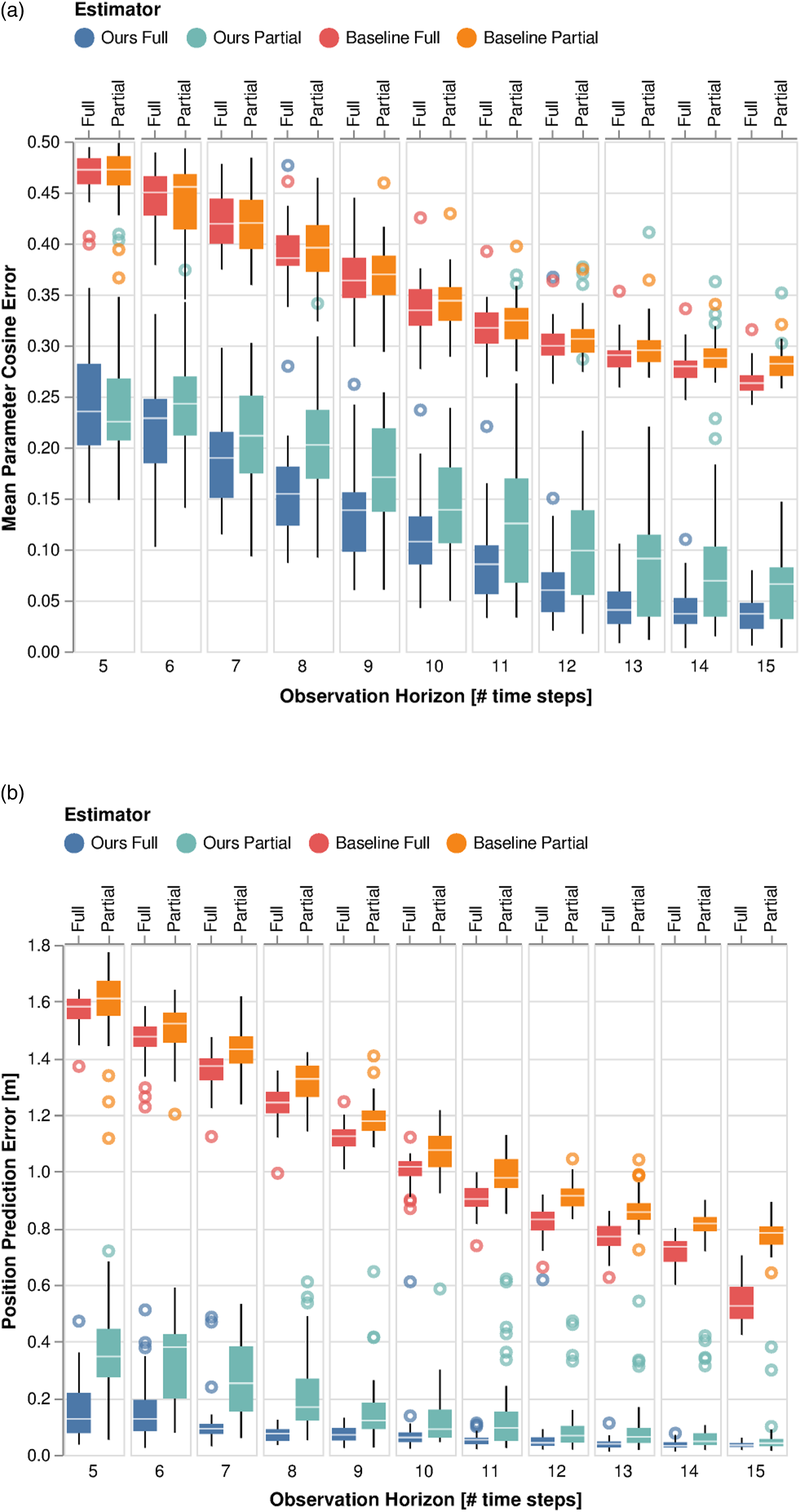

To inspect these results more closely, in Figure 6 we show the output of both methods for a single observation sequence of length $\stackrel{\sim }{\mathit{T}}=10$ . This visualization highlights a key advantage of our approach compared with the baseline. In this scenario, Player-2 (bottom) turns left early on in order to avoid Player-1 (left) later along the path to its goal. Their ground truth trajectories are shown in black. However, the methods only receive noise-corrupted partial state observations of the first $\stackrel{\sim }{\mathit{T}}=10$ time steps shown in gray. Our method models the players’ interactions as continuing into the future, allowing it to attribute observed behavior to future costs. In this instance, our method correctly explains Player-2’s observed left turn as the result of a modest penalty on proximity, which becomes important only later in the trajectory when the players are close to one another. Cost estimation is shown at the bottom of Figure 6. The KKT residual baseline is incapable of such attributions. More precisely, it can only consider the KKT residuals G (⋅; θ) of equation (21) for time steps $t\in \left[\stackrel{\sim }{\mathit{T}}\right]$ . Hence, the baseline must presume that the game terminates at $\stackrel{\sim }{\mathit{T}}$ rather than at some time in the future. Thus, it cannot anticipate the immediate future consequences of particular cost models. In Figure 6, the baseline can only explain the players’ early observed collision avoidance maneuver with an extremely large penalty on proximity to their opponents. As a result, it predicts that the players will quickly drive away from one another. Unlike our method, the baseline’s prediction rapidly diverges from the ground truth.

Figure 6.

Qualitative prediction performance of our method and the baseline for the 2-player collision-avoidance example when only the first 10 out of 25 time steps are observed.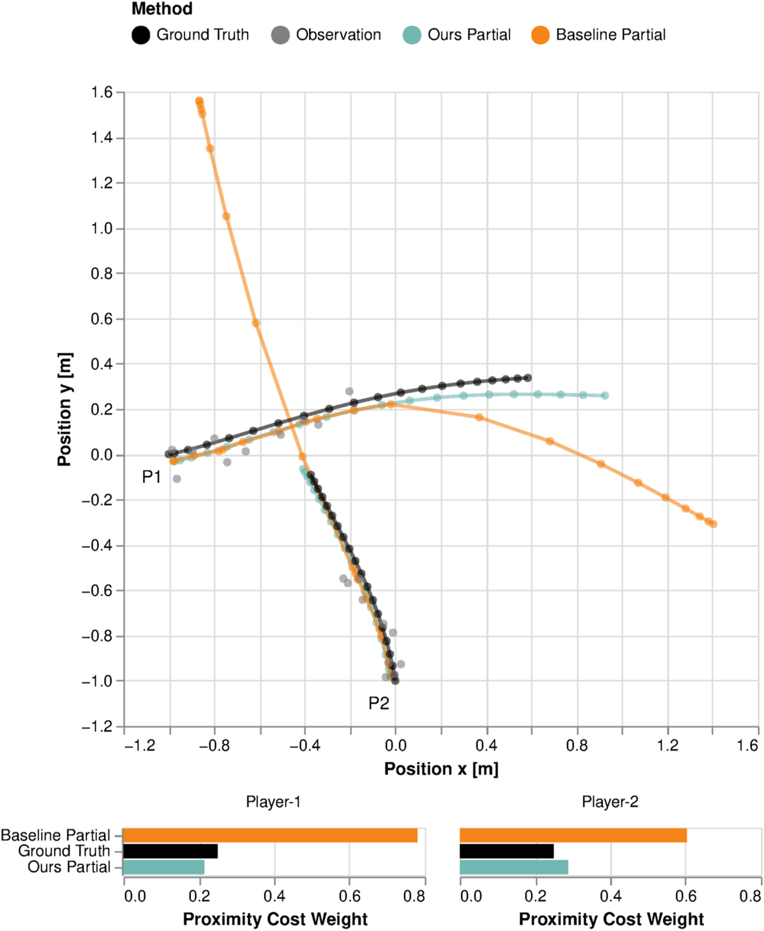

Beyond inference and prediction accuracy, a key factor for online operation is the computational complexity. To investigate this point, Figure 7 shows the computation time of both methods for the same dataset underpinning Figure 5. These timing results were obtained on an AMD Ryzen 9 5900HX laptop CPU. Overall, we observe that the KKT residual baseline has a lower runtime than our approach. The reduced runtime can be attributed to the fact that, by fixing the states and inputs a priori, the KKT residual formulation yields a simpler convex optimization problem in equation (21). Nonetheless, our method’s runtime still remains moderate and scales gracefully with the observation horizon. We note that our current implementation is not optimized for speed. In practical applications in the context of receding-horizon applications—a topic that we shall discuss in Section 7.3.2-the runtime may be further reduced via improved warm-starting and memory sharing across planner invocations.

Figure 7.

Runtime of our method and the baseline for varying numbers of observations of the 2-player collision-avoidance example at a fixed noise level of σ = 0.05.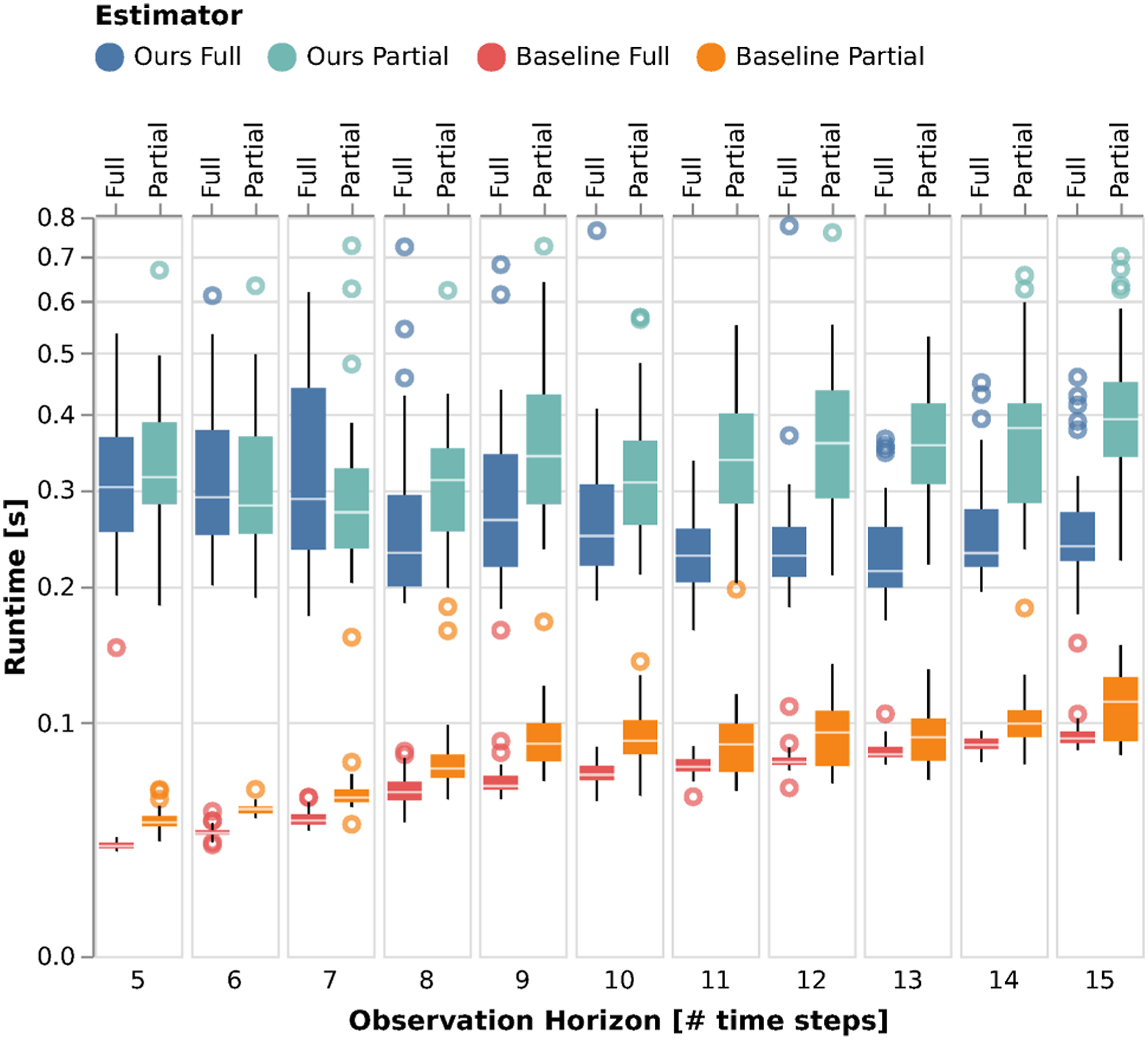

7.3. Scaling to larger games

While our approach is more easily analyzed in the small, two-player collision-avoidance game of Section 7.2, it readily extends to larger multi-agent interactions. In order to demonstrate scalability of the approach, we therefore replicate the offline learning analysis of Section 7.2.1 in a larger 5-player highway driving scenario depicted in Figure 1. Finally, we demonstrate a proof of concept for online, receding horizon learning in this scaled setting following the setup of Section 5.2.

In the highway scenario discussed through the remainder of this section, each player wishes to make forward progress in a particular lane at an unknown nominal speed, rather than reach a desired position as above. Therefore, ground-truth objectives use a quadratic penalty on deviation from a desired state that encodes each player’s target lane and preferred travel speed rather than a specific goal location. Despite these differences, this class of objectives is still captured by the cost structure introduced in equation (23e).

7.3.1. Offline learning

First, we study the performance of our method and the KKT residual baseline in the setting of offline learning without trajectory prediction. Figure 8 displays these results, using the same metrics as in Section 7.2.1 to measure performance in parameter space-Figure 8(a)-and position space-Figure 8(b). As before, our method demonstrably outperforms the baseline in both fully and partially observed settings. Furthermore, whereas our method performs comparably according to both metrics in the full and partial observation settings, the baseline performance differs between the two metrics. That is, while the performance of the baseline measured in parameter space is not significantly affected by less informative observations, the effect is significant in trajectory space. This inconsistency can be attributed to the fact that certain objective parameters have stronger influence on the resulting game trajectory than others. Since our method’s objective is observation fidelity, here measured by the measurement likelihood of equation (subsection 13a), it directly accounts for these varying sensitivities. The baseline, however, greedily optimizes the KKT residual of equation (21), irrespective of the resulting equilibrium trajectory.

Figure 8.

Estimation performance of our method and the baseline for the 5-player highway overtaking example, with noisy full and partial state observations. (a) Error measured directly in parameter space using equation (24). (b) Error measured in position space using equation (25). Triangular data markers in (b) highlight objective estimates which lead to ill-conditioned games. Solid lines and ribbons indicate the median and IQR of the error for each case.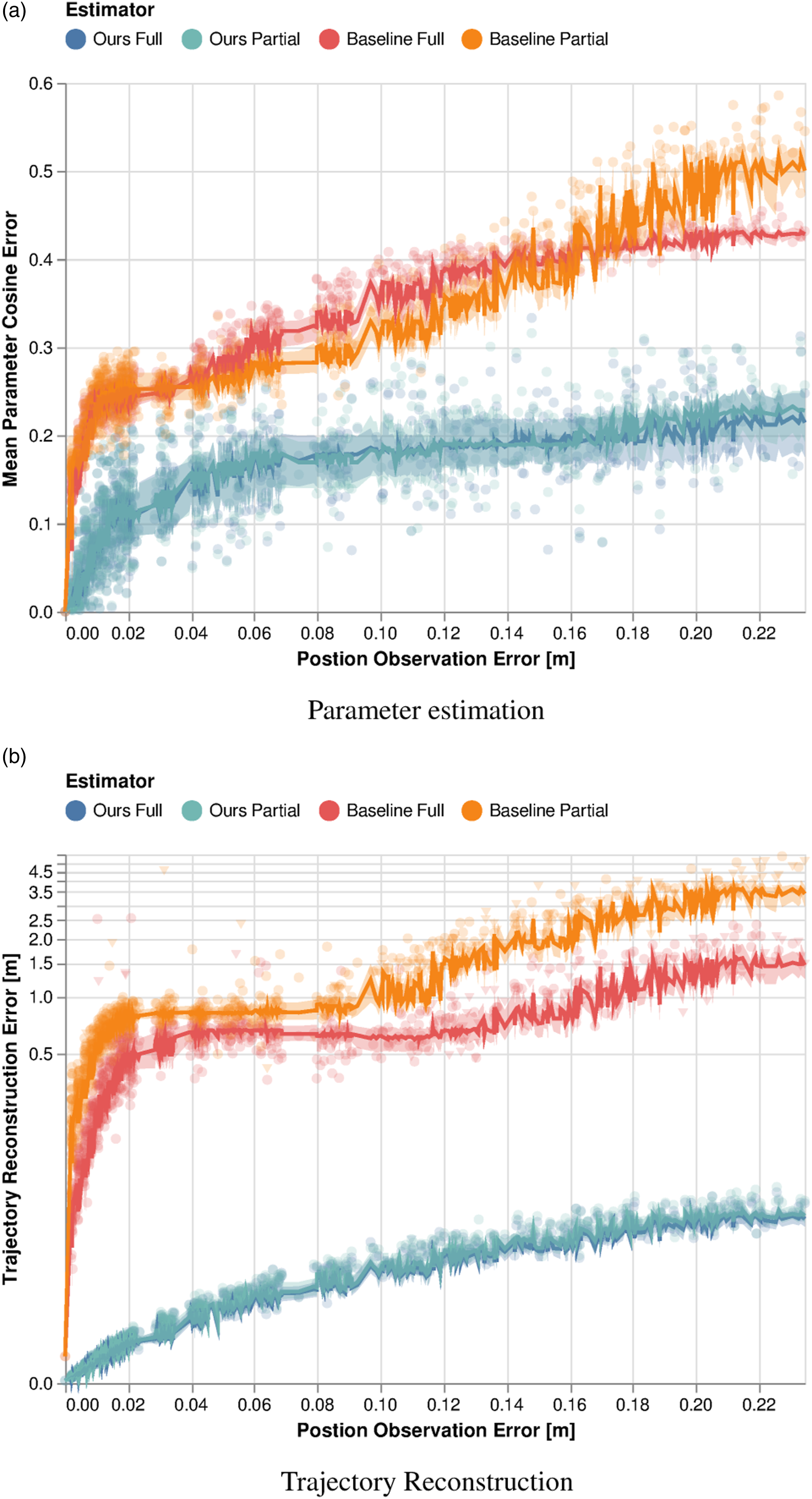

7.3.2. Online learning and receding horizon prediction

Finally, we demonstrate the application of our method for simultaneous online learning and receding-horizon prediction in the 5-player highway navigation scenario depicted in Figure 1.

Here, the information available to the estimator evolves over time and the problem only admits access to past observations of the game state for cost learning. Following the proposed procedure of Section 5.2, here, we limit the computational complexity of the estimation problem by considering only a fixed-lag buffer of observations over the last 5s and predict all player’s behavior over the next 10s. The qualitative performance of our method under noise-corrupted partial state observation is shown in Figure 9. As can be seen, from only a few seconds of data, our method learns player objectives that accurately predict the evolution of the game over a receding prediction horizon. Note that, by design, objective learning and behavior prediction are achieved simultaneously by solving a single joint optimization problem as in equation (13a). This ability to couple online learning and prediction makes it particularly suitable for online applications.

Figure 9

. Demonstration of our method in an online application of simultaneous objective learning and trajectory prediction for the 5-player highway navigation scenario. At each time step, objective learning is performed on a fixed-lag buffer of 5s of observation data which is coupled with trajectory prediction 10s into the future.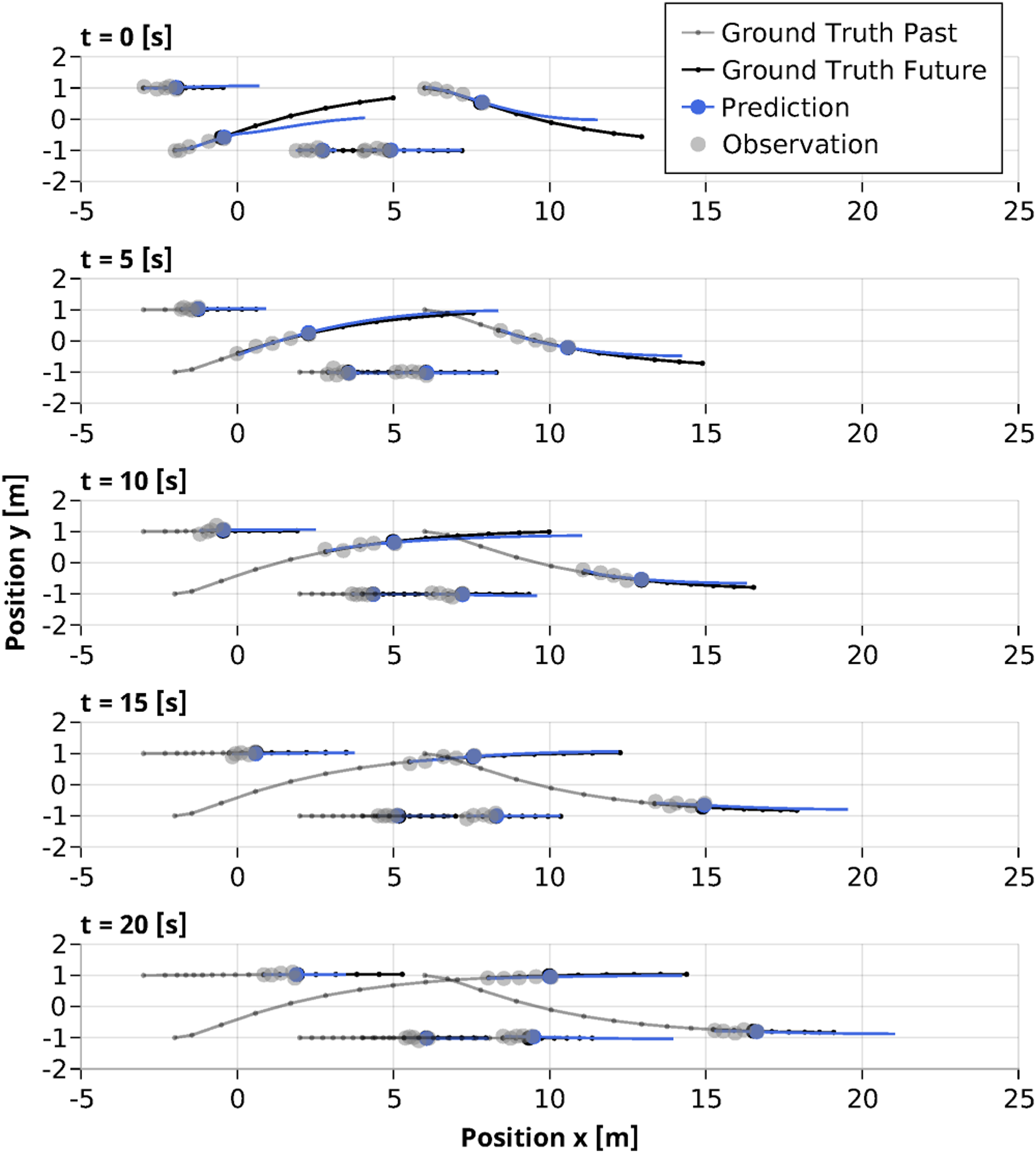

8. Conclusion

In this paper, we have introduced a novel approach to learn the parameters of players’ objectives in dynamic, noncooperative interactions, given only noisy, partial observations. This inverse dynamic game arises in a wide variety of multi-robot and human–robot interactions and generalizes well-studied problems such as inverse optimal control, inverse reinforcement learning, and learning from demonstrations. Contrary to prior work, our method learns players’ cost parameters while simultaneously recovering the forward game trajectory consistent with those parameters, with overall performance measured according to observation fidelity. We have shown how this formulation naturally extends to both offline learning and prediction problems, as well as online, receding horizon learning.

We have conducted extensive numerical simulations to characterize the performance of our method and compare it to a state-of-the-art baseline method (Rothfuß et al., 2017; Awasthi and Lamperski 2020). These simulations clearly demonstrate our method’s improved robustness to both observation noise and partial observations. Indeed, existing methods presume noiseless, full-state observations and thus require a priori estimation of states and inputs. Our method recovers objective parameters, reconstructs past game trajectories, and predicts future trajectories far more accurately than the baseline. Beyond that, our method’s structure allows to perform all of these tasks jointly as the solution of a single optimization problem. This feature renders our method suitable for online learning and prediction in a receding horizon fashion.

In light of these encouraging results, there are several directions for future research. Most immediately, our method lends itself naturally to deployment onboard physical robotic systems such as the autonomous vehicles considered in the examples of Section 7. In particular, the online, receding horizon learning and prediction procedure of Section 5.2 may be run onboard an autonomous car. Here, the “ego” agent would seek to learn other vehicles’ objective parameters while simultaneously using the receding horizon game solution to respond to predicted opponent strategies.

Another exciting, more theoretical direction consists of extending our formulation to more complex equilibrium concepts than OLNE. For example, recent solution methods for forward games in state feedback Nash equilibria (Fridovich-Keil et al., 2020; Laine et al., 2021; Di and Lamperski 2021) might be adapted to solve inverse games along the lines of equation (12a).