Asymptotically optimal inspection planning via efficient near-optimal search on sampled roadmaps

Abstract

Inspection planning, the task of planning motions for a robot that enable it to inspect a set of points of interest, has applications in domains such as industrial, field, and medical robotics. Inspection planning can be computationally challenging, as the search space over motion plans grows exponentially with the number of points of interest to inspect. We propose a novel method, Incremental Random Inspection-roadmap Search (IRIS), that computes inspection plans whose length and set of successfully inspected points asymptotically converge to those of an optimal inspection plan. IRIS incrementally densifies a motion-planning roadmap using a sampling-based algorithm and performs efficient near-optimal graph search over the resulting roadmap as it is generated. We prove the resulting algorithm is asymptotically optimal under very general assumptions about the robot and the environment. We demonstrate IRIS’s efficacy on a simulated inspection task with a planar five DOF manipulator, on a simulated bridge inspection task with an Unmanned Aerial Vehicle (UAV), and on a medical endoscopic inspection task for a continuum parallel surgical robot in cluttered human anatomy. In all these systems IRIS computes higher-quality inspection plans orders of magnitudes faster than a prior state-of-the-art method.

1. Introduction

In this work, we investigate the problem of inspection planning, or coverage planning (Almadhoun et al., 2016; Galceran and Carreras 2013). Here, we consider the specific setting where we are given a robot equipped with a sensor and a set of points of interest (POI) in the environment to be inspected by the sensor. The problem calls for computing a minimal-length motion plan for the robot that maximizes the number of POI inspected. This problem has a multitude of diverse applications, including surface inspections in industrial production lines (Raffaeli et al., 2013), surveying the ocean floor by autonomous underwater vehicles (Bingham et al., 2010; Gracias et al., 2013; Johnson-Roberson et al., 2010; Tivey et al., 1997), structural inspection of bridges using aerial robots (Bircher et al., 2015, 2016), and medical applications such as inspecting patient anatomy during surgical procedures (Kuntz et al., 2018).

Naïvely computed inspection plans may enable inspection of only a subset of the POI and may require motion plans orders of magnitude longer than an optimal plan, and hence may be undesirable or infeasible due to a robot’s battery capacity or time constraints. In medical applications, physicians may want to maximize the number of POI inspected for diagnostic purposes. Additionally, the procedure should be completed as fast as is safely possible to reduce costs and improve patient outcomes, especially if the patient is under anesthesia during the procedure. For example, a robot assisting in the diagnosis of the cause of a pleural effusion (a serious medical condition that can cause the collapse of a patient’s lung) will need to visually inspect the surface of the collapsed lung and chest wall inside the body in as short a time as possible (see Figure 1(a)). In structural inspecting applications, Unmanned Aerial Vehicles (UAVs), or drones, can be used to efficiently inspect the complex geometry of built structures. High-quality inspection plans could reduce inspection time and reduce costs. Bridge inspection (see Figure 1(b)), for example, is critical to ensuring bridge safety since almost 40% of the bridges in the United States exceed their 50-year design life (ASCE 2016). We note that it may not be possible to inspect some POI due to obstacles in the environment and the kinematic constraints of the robot. Our goal is to compute kinematically feasible collision-free inspection plans that maximize the number of POI inspected, and of the motion plans that inspect those POI we compute a shortest plan.

Figure 1.

Examples of applications of inspection planning. (a) Inspection planning in human anatomy. Left: The Continuum Reconfigurable Incisionless Surgical Parallel (CRISP) robot (Anderson et al., 2017; Mahoney et al., 2016) is composed of needle-diameter tubes assembled into a parallel structure inside the patient’s body (in which a tube uses a snare system to grip a tube with a camera affixed to its tip) and then robotically manipulated outside the body, allowing for smaller incisions and faster recovery times compared to traditional endoscopic tools (which have larger diameters). Middle: The CRISP robot in simulation inspecting a collapsed lung, a scenario segmented from a CT scan of a real patient with this condition. The visualization shows the robot (orange), the lungs (pink), and the pleural surface visible (green) and not visible (blue) by the robot’s camera sensor in its current configuration. Right: Two example configurations with inspected POI. The CRISP robot (orange) inspects POI (blue) on the organ surface, and visible points are covered by the cone shape (yellow). (b) Inspection planning for bridge structures. A UAV, shown as a blue sphere, inspects points on the surface of a bridge structure. At a configuration, some points are visible (shown in green) while other points are not visible (shown in orange).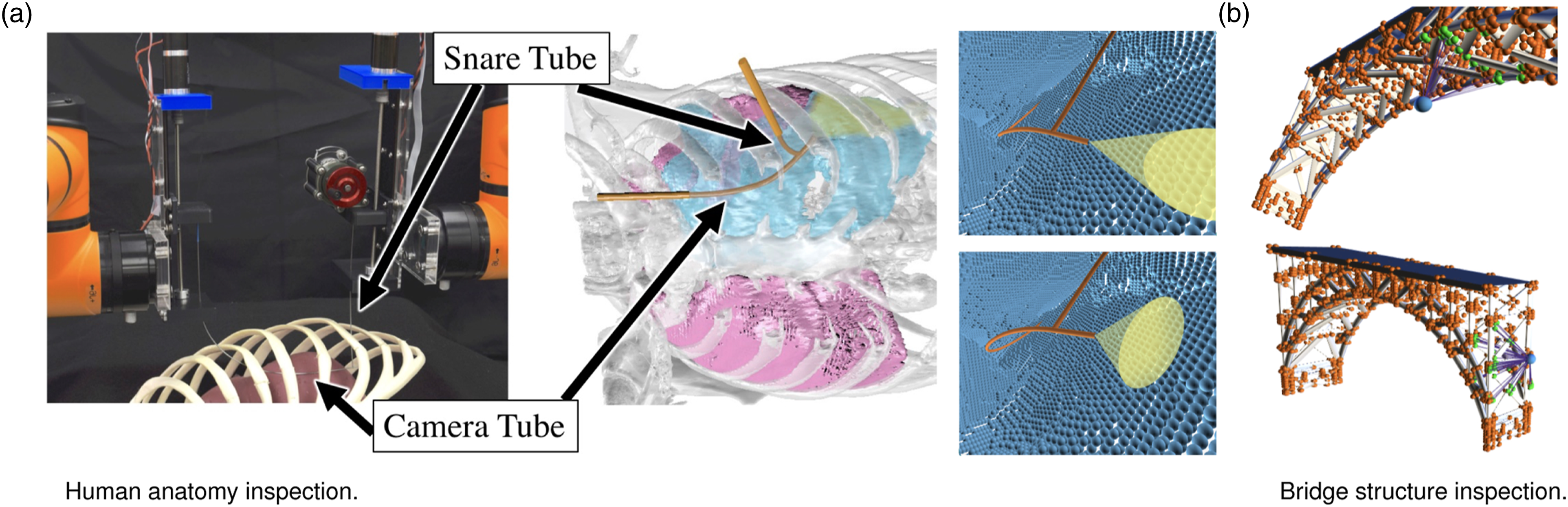

Inspection planning is computationally challenging because the search space is embedded in a high-dimensional configuration space $\mathcal{X}$ (the space of all parameters that determine the shape of the robot) (Choset et al., 2005; Latombe 1991; LaValle 2006). Even finding the shortest plan between two points in $\mathcal{X}$ that avoid obstacles (without reasoning about inspection) is computationally hard. ¹ If we want to compute a minimum-length motion plan that maximizes the number of POI inspected, the complexity of our problem is increased as we have to simultaneously reason about the system’s constraints, motion plan length, and POI inspected.

There are multiple approaches to computing inspection plans. Optimization-based methods locally search over the space of all inspection plans (Bircher et al., 2015; Bogaerts et al., 2018). Decoupled approaches first independently select suitable viewpoints and then determine a visiting sequence, that is, a motion plan for the robot that realizes this sequence (Danner and Kavraki 2000; Englot and Hover 2011). Finally, recent progress in motion planning (Karaman and Frazzoli 2011) has enabled methods to exhaustively search over the space of all motion plans (Bircher et al., 2017; Kafka et al., 2016; Papadopoulos et al., 2013) thus guaranteeing asymptotic optimality, an important feature in many applications, including medical ones. Roughly speaking, asymptotic optimality for inspection planning means these methods produce inspection plans whose length and the number of points inspected will asymptotically converge to those of an optimal inspection plan, given enough planning time.

Of all the aforementioned methods, only algorithms in the latter group provide any formal guarantees on the quality of the solution. This guarantee is achieved by attempting to exhaustively compute the set of Pareto-optimal inspection plans embedded in $\mathcal{X}$ for which full coverage has not been obtained. Namely, for every configuration $\mathbf{q}\in \mathcal{X}$ , they (asymptotically) compute the set of paths Π _q ending at q and starting from a given start configuration q _s such that ∀π ₁ , π ₂ ∈ Π _q , either π ₁ is shorter than π ₂ and π₂ covers POI not covered by π₁ or vice versa. Once Π _q contains a path ${\pi }_{\mathbf{q}}^{\ast }$ that covers all POI, this path is considered as a candidate solution. In our setting, the set of Pareto-optimal inspection plans is the minimal set of inspection plans such that each plan is either shorter or has better coverage of the POI than any other inspection plan. ² Unfortunately, this comes at the price of very long computation times as the size of the search space is exponential in the number of POI.

To this end, we introduce Incremental Random Inspection-roadmap Search (IRIS), a new asymptotically optimal inspection-planning algorithm. IRIS incrementally constructs a sequence of increasingly dense roadmaps—graphs embedded in $\mathcal{X}$ wherein each vertex represents a collision-free configuration and each edge a collision-free transition between configurations—and computes an inspection plan on the roadmaps as they are constructed (see Figure 2).

Figure 2.

Overview of the IRIS algorithmic framework.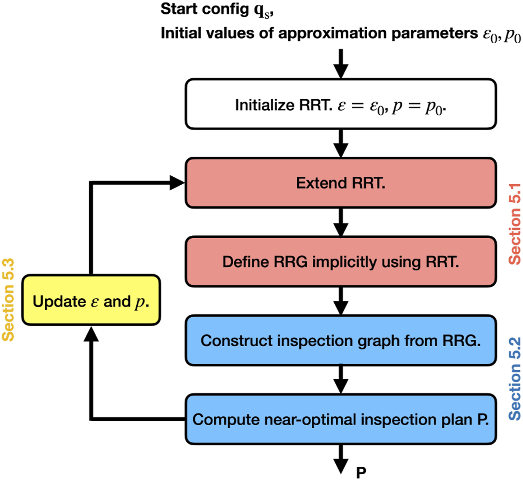

Unfortunately, even the problem of computing an optimal inspection plan on a graph (and not in the continuous space) is computationally hard. To this end, our key insight is to compute a near-optimal inspection plan on each roadmap. Namely, we compute an inspection plan that is at most 1 + ɛ the length of an optimal plan while covering at least p-percent of the number of POI (for any ɛ ≥ 0 and p∈(0,1]). This additional flexibility allows us to improve the quality of our inspection plan in an anytime manner, that is, the algorithm can be stopped at any time and return the best inspection plan found up until that point. We achieve this by incrementally densifying the roadmap and then searching over the densified roadmap for a near-optimal inspection plan—a process that is repeated as time allows. By reducing the approximation factor between iterations, we ensure that our method is asymptotically optimal.

The key contribution of our work is a computationally efficient algorithm to compute provably near-optimal inspection plans on graphs. Coupled with our method for generating this graph, this algorithmic building block enables us to dramatically outperform Rapidly-exploring Random Tree Of Trees (RRTOT) (Bircher et al., 2017)—a state-of-the-art asymptotically optimal inspection planner. Specifically, we demonstrate the efficacy of our approach in simulation for several complex robotic systems (Figure 1), including a continuum robot with complex kinematics—the needle-diameter Continuum Reconfigurable Incisionless Surgical Parallel (CRISP) robot (Anderson et al., 2017; Mahoney et al., 2016), working in a medically inspired setting involving the diagnosis of a pleural effusion.

In this paper, we are providing a refined version of our results in Fu et al. (2019), and two important extensions. First, we show results for a simulated bridge inspection task with a UAV, where the inspection target has a complex structure and the underlying roadmap to compute a near-optimal inspection plan on is much larger (e.g., having more nodes and edges). Second, we prove that IRIS is asymptotically optimal under very general system and environment assumptions. These extensions show that IRIS can be used for general complex-structure inspection while providing provable guarantees.

2. Related Work

2.1. Sampling-based motion planning

Motion planning algorithms aim to compute a collision-free motion for a robot to accomplish a task in an environment cluttered with obstacles (Halperin et al., 2018; LaValle 2006; Lynch and Park 2017). A common approach to motion planning is by sampling-based algorithms that construct a roadmap. Examples include the Probabilistic Roadmaps (PRMs) (Kavraki et al., 1996) (often for solving multiple queries) and the Rapidly-exploring Random Trees (RRTs) (LaValle and Kuffner 2001) for solving single queries. These methods, and many variations thereof, are probabilistically complete—namely, the likelihood that they will find a solution, if one exists, approaches certainty as computation time increases.

Recent variations of these methods, such as PRM* and RRT* (Karaman and Frazzoli 2011), improve upon this guarantee by exhibiting asymptotic optimality—namely, that the quality of the solution obtained, given some cost function, approaches the global optimum as computation increases. Roughly speaking, this is achieved by increasing the (potential) edge set of roadmap vertices considered as its size increases (Karaman and Frazzoli 2011; Solovey et al., 2018). One such algorithm is the Rapidly-exploring Random Graphs (RRGs) (Karaman and Frazzoli 2011) which will be used in our work. RRG combines the exploration strategy of RRT with an updated connection strategy that allows for cycles in the roadmap. It requires solving the two-point boundary value problem (LaValle 2006), which is only efficiently solvable for some robotic systems (including ours).

Guaranteeing asymptotic optimality can come with a heavy computational cost. This inspired work on planners that trade asymptotic optimality guarantees with asymptotic near optimality (e.g., Li et al. (2016); Marble and Bekris (2011); Salzman and Halperin (2016)). Asymptotic near optimality states that given an approximation factor ɛ ≥ 0, the solution obtained converges to within a factor of (1 + ɛ) of the optimal solution with probability one, as the number of samples tends to infinity. Relaxing optimality to near optimality allows a method to improve the practical convergence rate while maintaining desired theoretic guarantees on the quality of the solution.

2.2. Inspection planning

Many inspection-planning algorithms, or coverage planners, decompose the region containing the POI into multiple sub-regions and then solve each sub-region separately (Galceran and Carreras 2013). These methods have limitations, however, such as when occlusions play a significant role in the inspection (Englot and Hover 2012), or when kinematic constraints must be considered (Edelkamp et al., 2017).

Other approaches simultaneously consider all POI. One approach decouples the problem into the coverage sampling problem (CSP) and the multi-goal planning problem (MPP), and solves each independently (Bircher et al., 2015; Danner and Kavraki 2000; Edelkamp et al., 2017; Englot and Hover, 2011, 2012). In CSP, a minimal set of viewpoints that provide full inspection coverage is computed. In MPP, a shortest tour that connects all the viewpoints is computed. These correspond to solving the art gallery problem and the traveling salesman problem, respectively. Several of these variants have been shown to be probabilistically complete (Englot and Hover 2012), but none provide guarantees on the quality of the final solution.

The set of viewpoints and the inspection plan itself can also be generated simultaneously. Papadopoulos et al. (2013) propose the Random Inspection Tree Algorithm (RITA). RITA takes into account the differential constraints of the robot and computes both target points for inspection and the trajectory to visit the targets simultaneously. Bircher et al. (2017) propose Rapidly-exploring Random Tree Of Trees (RRTOT) which constructs a meta–tree structure consisting of multiple RRT* trees. Both methods, which were shown to be asymptotically optimal, iteratively generate a tree, in which the inspection plan is enforced to be a plan from the root to a leaf node. However, each inspection plan does not consider configurations from other branches in the tree which may cause long planning times. This motivates our RRG-based approach.

2.3. Path planning on graphs

Planning a minimal-cost path on a graph is a well-studied problem. When the cost function has an optimal substructure (namely, when subpaths of an optimal path are also optimal), efficient algorithms such as Dijkstra (Dijkstra 1959), A* (Hart et al., 1968), and the many variants thereof can be used. However, in certain settings, including ours, this is not the case. For example, Tsaggouris and Zaroliagis (2004) consider the case where every edge has two attributes (e.g., cost and resource), and the cost function incorporates the attributes in a non-linear fashion.

It is worth mentioning the idea of progressively tightening the approximation factor was also adopted in some anytime A* algorithms based on weighted A* (Pohl 1970), including Anytime Repairing A* (ARA*) by Likhachev et al. (2003) and Restarting Weighted A* (RWA*) by Richter et al. (2010). Anytime Nonparametric A* (ANA*) by van Den Berg et al. (2011) furthermore gets rid of the explicit approximation parameter and performs solution improvement adaptively. Nevertheless, as these methods are based on weighted A*, a prerequisite for good performance is a high-quality heuristic, which is not easy to obtain in the case of inspection planning due to the lack of optimal substructure. Furthermore, these methods focus on static graphs (while in our case the graph is incrementally updated) and consider only a single objective (while in our case we have two objectives, inspection and path length). When looking at multiple objectives (though still considering static graphs), recent work by Zhang et al. (2022) extends the approach presented in this paper to suggest an anytime approximate bi-criteria search algorithm.

Inspection planning also bears resemblance to multi-objective path planning. Here, we are given a set of cost functions and are required to find the set of Pareto-optimal paths (Pardalos et al., 2008). Unfortunately, this set may be exponential in the problem size (Ehrgott and Gandibleux 2000). However, it is possible to compute a fully polynomial-time approximation scheme (FPTAS) for many cases (Tsaggouris and Zaroliagis 2009). For additional results on path planning with multiple objectives or when the cost function does not have an optimal substructure, see for example, (Chen and Nie 2013; Reinhardt and Pisinger 2011; Hernández et al., 2023) and references within.

3. Problem definition

In this section, we formally define the inspection planning problem. The robot operates in a workspace $\mathcal{W}\subset {\mathbb{R}}^3$ amidst a set of obstacles ${\mathcal{W}}_{\text{obs}}\subset \mathcal{W}$ . The robot’s configuration q is a d-dimensional vector that uniquely defines the shape of the robot (including, e.g., rotation angles and translational extension of all joints). The set of all such configurations is the configuration space $\mathcal{X}$ . The geometry of the robot is a configuration-dependent shape $\text{Shape}\left(\mathbf{q}\right)\subset \mathcal{W}$ , here, Shape(⋅) is a mapping from configuration space $\mathcal{X}$ to workspace $\mathcal{W}$ , determining the subset of the workspace that the robot occupies for a given configuration. We say that $\mathbf{q}\in \mathcal{X}$ is in collision if $\text{Shape}\left(\mathbf{q}\right)\hspace{0.17em}\cap \hspace{0.17em}{\mathcal{W}}_{\text{obs}}\ne$ . Let ${\mathcal{X}}_{\text{obs}}\subseteq \mathcal{X}$ be the obstacle space, such that $\mathcal{X}\setminus {\mathcal{X}}_{\text{obs}}$ is an open set. Then the collision-free space is defined as ${\mathcal{X}}_{\text{free}}=\text{cl}\left(\mathcal{X}\setminus {\mathcal{X}}_{\text{obs}}\right)$ , where cl(⋅) is closure of a set. In this work we define a motion plan for the robot as a path P in $\mathcal{X}$ , which is represented as a sequence of n configurations {q₀, …, q_n−1} (vertices) connected by straight-line segments (edges) in $\mathcal{X}$ . And we say that P is collision-free if all configurations along P (vertices and edges) are collision-free. We assume that we have a distance function $\mathit{\ell }:\mathcal{X}\times \mathcal{X}\to \mathbb{R}$ and denote the length of a path P as the sum of the distances between consecutive vertices, i.e., ℓ(P)≔∑ _i ℓ(q _i , q_i−1).

We assume that the robot is equipped with a sensor $\mathcal{S}$ and we are given a set of k points of interest (POI) $\mathcal{I}=\left\{i_1,\dots ,i_k\right\}$ in $\mathcal{W}$ . We model the sensor as a mapping $\mathcal{S}:\mathcal{X}\to 2^{\mathcal{I}}$ , where $2^{\mathcal{I}}$ is the power set of $\mathcal{I}$ and S denotes the subset of $\mathcal{I}$ that can be inspected from each configuration. By a slight abuse of notation, given a path P we set $\mathcal{S}\left(P\right):={\cup }_{i=0}^{n-1}\mathcal{S}\left({\mathbf{q}}_i\right)$ and note that in our model, we only inspect $\mathcal{I}$ along the vertices of a path.

Definition 1. Inspection coverage. A point of interest $i\in \mathcal{I}$ is said to be covered by a configuration $\mathbf{q}\in \mathcal{X}$ or by a path P if $i\in \mathcal{S}\left(\mathbf{q}\right)$ or if $i\in \mathcal{S}\left(P\right)$ , respectively. In such a setting, we say that q (or P) covers the point of interest i.

Given a start configuration ${\mathbf{q}}_{\mathrm{s}}\in \mathcal{X}$ , POI $\mathcal{I}$ , and a sensor model $\mathcal{S}$ , the inspection planning problem calls for computing a collision-free path P starting at q_s which maximizes $\left|\mathcal{S}\left(P\right)\right|$ while minimizing ℓ(P). Note that this is not a bicriteria optimization problem—our primary optimization function is maximizing the coverage of our path. Out of all such paths we are interested in the shortest one.

4. Method overview

In this section, we provide an overview of IRIS—our algorithmic framework for computing asymptotically optimal inspection plans. A key algorithmic tool in our approach is to cast the continuous inspection planning problem (Sec. 3) to a discrete version of the problem where we only consider a finite number of configurations from which we inspect the POI, and a discrete set of feasible movements between those configurations. The assumption that inspection of POI only happens at vertices is not significantly limiting since a robot’s motion can be approximated by multiple vertices, and many inspection applications require non-zero time to complete a high-quality sensor measurement (e.g., to obtain non-blurry images and high-accuracy lidar scans), which can be effectively encoded at vertices. Thus, we start in Sec. 4.1 by formally defining the graph inspection problem and then continue in Sec. 4.2 to provide an overview of how IRIS builds and uses such graphs. We then describe the method in detail in Sec. 5, and in Sec. 6 show that IRIS’s solution converges to the length and coverage of an optimal inspection path.

4.1. Graph inspection problem

Similar to the (continuous) inspection problem, a graph inspection problem is a tuple $\left(\mathcal{G},\mathit{\ell },\mathcal{S},\mathcal{\ell },v_{\mathrm{s}}\right)$ where $\mathcal{G}=\left(\mathcal{V},\mathcal{E}\right)$ is a motion-planning roadmap (namely, a graph embedded in $\mathcal{X}$ , in which every vertex $v\in \mathcal{V}$ is a configuration and every edge $\left(u,v\right)\in \mathcal{E}$ denotes the transition from configuration u to v), $\mathcal{I}$ and $\mathcal{S}$ are defined as in Sec. 3, $\mathit{\ell }:\mathcal{E}\to \mathbb{R}$ denotes the length of each edge in the roadmap, and v_s is the start vertex (corresponding to the start configuration q_s). A path P on $\mathcal{G}$ is represented by a sequence of vertices $v_i\in \mathcal{V}$ such that P = {v₀, …, v_n−1}, v₀ = v _s and $\left(v_i,v_{i+1}\right)\in \mathcal{E}$ . It is important to note that there can be loops in a path, so it is possible that v _m = v _k for m ≠ k. The length and coverage of P are defined as the total length of P’s edges and the set of all points inspected when traversing P, respectively. Namely, $\mathit{\ell }\left(P\right):={\sum }_{i=0}^{n-2}\mathit{\ell }\left(v_i,v_{i+1}\right)$ and $\mathcal{S}\left(P\right):=U_{v\in P}\hspace{0.17em}\mathcal{S}\left(v\right)$ . The optimal graph inspection problem calls for a path P* that starts at v_s and maximizes the number of points inspected. Out of all such paths, P* has the minimal length. Finally, a path is said to be near-optimal for some ɛ ≥ 0 and p∈(0,1] if $\left|\mathcal{S}\left(P\right)\right|/\left|\mathcal{S}\left(P^{*}\right)\right|\ge p$ and ℓ(P) ≤ (1 + ɛ) ⋅ ℓ(P*).

4.2. Overview of IRIS

Our algorithmic framework, depicted in Figure 2, interleaves sampling-based motion planning and graph search. Specifically, we incrementally construct an RRT $\mathcal{T}$ rooted at q_s which implicitly defines a corresponding RRG $\mathcal{G}$ . All edges in $\mathcal{T}$ are checked for collision with the environment during its construction (so the roadmap is guaranteed to be connected) while all the other edges of $\mathcal{G}$ are not explicitly checked for collision. Lazy edge evaluation, common in motion-planning algorithms (Bohlin and Kavraki 2000; Hauser 2015; Dellin and Srinivasa 2016; Salzman and Halperin 2015), allows us to defer collision detection until absolutely necessary and reduce computational effort. This is critical in our domain of interest where computing Shape(⋅), the geometry of the robot as is defined in Sec. 3, typically dominates algorithms’ running times (Niyaz et al., 2018).

The roadmap $\mathcal{G}=\left(\mathcal{V},\mathcal{E}\right)$ induces the subset of the POI that can be inspected, denoted as ${\mathcal{I}}_{\mathcal{G}}:=\underset{v\in \mathcal{V}}{\cup }\mathcal{S}\left(v\right)$ . Given two approximation parameters ɛ ≥ 0 and p∈(0,1], we compute a near-optimal inspection path for the graph inspection problem $\left(\mathcal{G},{\mathcal{I}}_{\mathcal{G}},\mathcal{S},\mathit{\ell },v_{\mathrm{s}}\right)$ by casting the problem as a graph-search problem on a different graph ${\mathcal{G}}_{\mathcal{S}}$ (to be defined shortly).

As we add vertices and edges to $\mathcal{T}$ incrementally, the roadmap $\mathcal{G}$ is incrementally densified. In addition, we tighten approximations by decreasing ɛ and increasing p between iterations. As we will see (Sec. 6), this will ensure that IRIS is asymptotically optimal.

5. Method

In this section, we detail the different components of IRIS. Sections 5.1 and 5.2 describe how we construct a roadmap and then search it, respectively. After describing in Sec 5.3 how we modify the approximation parameters used by IRIS, we conclude in Sec. 5.4 with implementation details.

5.1. Roadmap construction

We construct a sequence of graphs embedded in $\mathcal{X}$ . Specifically, denote the RRT constructed at the i’th iteration as ${\mathcal{T}}_i$ defined over the set of vertices ${\mathcal{V}}_i$ . We start with an empty tree rooted at q_s and at the i’th iteration sample a random configuration, compute its nearest neighbor in ${\mathcal{T}}_i$ , and extend that vertex toward the random configuration. If that extension is collision-free we add it to the tree. If not, we repeat this process (see Kuffner and LaValle (2000); LaValle (2006) for additional details regarding RRT).

Note that it is not necessary to add only one collision-free configuration in each roadmap update. Adding multiple configurations in one iteration does not hurt the theoretical guarantees while providing us more room to improve an inspection plan in terms of both inspection and path length. There are different possible strategies to balance between roadmap construction and graph search on the roadmap. One example is Fu et al. (2021) where a condition on additional inspection coverage is used to trigger graph searches on the updated roadmap. As the major focus of this paper is to provide a theoretical foundation for the proposed algorithm framework, we only discuss the variant where configurations are added one at a time.

The tree ${\mathcal{T}}_i$ implicitly defines an RRG $G_i=\left({\mathcal{V}}_i,{\mathcal{E}}_i\right)$ defined over the same set of vertices where every vertex is connected to all other vertices within distance r _i . Here, we define r _i as in Lemma 3 which will allow us to prove that our approach is asymptotically optimal (see Sec. 6).

5.2. Graph inspection planning

We use the RRG described in Sec. 5.1 to define a graph inspection problem, and then compute near-optimal inspection paths over this graph. Before describing how we compute near-optimal inspection paths, we first describe how we compute optimal paths given a graph inspection problem.

5.2.1. Optimal planning

Given a graph inspection problem $\left(\mathcal{G},{\mathcal{I}}_{\mathcal{G}},\mathcal{S},\mathit{\ell },v_{\mathrm{s}}\right)$ , we compute optimal inspection paths by formulating our inspection problem as a graph-search problem on an inspection graph ${\mathcal{G}}_{\mathcal{S}}:=\left({\mathcal{V}}_{\mathcal{S}},{\mathcal{E}}_{\mathcal{S}}\right)$ . Here, vertices are pairs comprised of a vertex $u\in \mathcal{V}$ in the original graph and subsets of ${\mathcal{I}}_{\mathcal{G}}$ . Namely, ${\mathcal{V}}_{\mathcal{S}}=\mathcal{V}\times 2^{{\mathcal{I}}_{\mathcal{G}}}$ , and note that $\left|{\mathcal{V}}_{\mathcal{S}}\right|=O\left(\left|\mathcal{V}\right|·2^{\left|{\mathcal{I}}_{\mathcal{G}}\right|}\right)$ . An edge e between vertices $\left(u,{\mathcal{I}}_u\right)$ and $\left(v,{\mathcal{I}}_v\right)$ exists if $\left(u,v\right)\in \mathcal{E}$ and ${\mathcal{I}}_u\hspace{0.17em}\cup \hspace{0.17em}\mathcal{S}\left(v\right)={\mathcal{I}}_v$ . If it exists, its cost is simply ℓ(u, v).

Any (possibly non-simple) path P _G in the original graph G from v_s to u can be represented by a corresponding path $P_{{\mathcal{G}}_{\mathcal{S}}}$ in the inspection graph ${\mathcal{G}}_{\mathcal{S}}$ , from $\left(v_{\mathrm{s}},\mathcal{S}\left(v_{\mathrm{s}}\right)\right)\in {\mathcal{V}}_{\mathcal{S}}$ to $\left(u,\mathcal{S}\left(P_G\right)\right)\in {\mathcal{V}}_{\mathcal{S}}$ , and $\mathit{\ell }\left(P_G\right)=\mathit{\ell }\left(P_{{\mathcal{G}}_{\mathcal{S}}}\right)$ . Thus, our algorithm will run an A*-like search from $\left(v_{\mathrm{s}},\mathcal{S}\left(v_{\mathrm{s}}\right)\right)\in {\mathcal{V}}_{\mathcal{S}}$ to any vertex in the goal set ${\mathcal{V}}_{\text{goal}}=\left\{\left(v,{\mathcal{I}}_{\mathcal{G}}\right)|v\in \mathcal{V}\right\}$ . An optimal inspection path is the shortest path between $\left(v_{\mathrm{s}},\mathcal{S}\left(v_{\mathrm{s}}\right)\right)$ and any vertex in ${\mathcal{V}}_{\text{goal}}$ . For a visualization, see Figure 3. Note that here we assume the graph $\mathcal{G}$ is connected and that the set of points to be inspected is ${\mathcal{I}}_{\mathcal{G}}$ . This implies that an optimal inspection path always exists.

Figure 3.

Computing optimal inspection paths on graphs by casting a graph-inspection problem (bottom) to a graph-search problem (top). Gray layers correspond to the set of all vertices in ${\mathcal{V}}_{\mathcal{S}}$ that share the same set of points inspected. Edges connecting vertices in the same (different) layer are depicted in dashed (dotted) lines, respectively. The start is (a, ) and the goal set ${\mathcal{V}}_{\text{goal}}$ contains all vertices in the top layer. Notice that the optimal path (blue) visits vertex a twice.

We can speed up this naïve algorithm using the notion of dominance, which is used in many shortest-path algorithms (see, e.g., Salzman et al. (2017)). In our context, given two paths P, P′ in our original roadmap $\mathcal{G}$ that start and end at the same vertices, we say that P dominates P′ if ℓ(P) ≤ ℓ(P′) and $\mathcal{S}\left(P\right)\supseteq \mathcal{S}\left(P^{\prime }\right)$ . Clearly, P is always preferred over P′. Thus, when searching ${\mathcal{G}}_{\mathcal{S}}$ , if we compute a shortest path to some node $\left(u,{\mathcal{I}}_u\right)$ of length ℓ _u , we do not need to consider any path of length larger than ℓ _u from all vertices $\left(u,{\mathcal{I}}_u^{\prime }\right)$ such that ${\mathcal{I}}_u^{\prime }\subseteq {\mathcal{I}}_u$ . For pseudo-code describing a general A*-like search algorithm to optimally solve the graph inspection problem, see Alg. 1 without lines 17-27.

While path domination may prune away paths in the open list of the A* -like search, this algorithm is hardly practical due to the exponential size of the search space (recall that $\left|{\mathcal{V}}_{\mathcal{S}}\right|=O\left(\left|{\mathcal{V}}_{\mathcal{S}}\right|·2^{\left|{\mathcal{I}}_{\mathcal{G}}\right|}\right)$ ). In the next sections, we show how to prune away large portions of the search space by extending the notion of dominance to approximate dominance.

5.2.2. Near-optimal planning

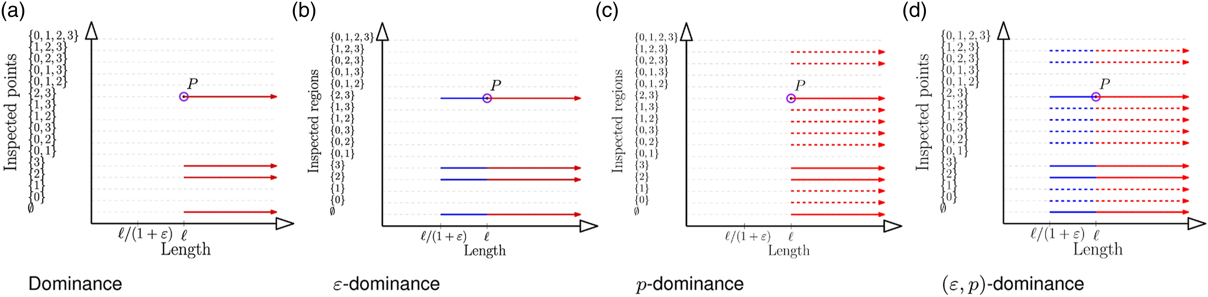
To perform near-optimal planning, we introduce the idea of approximate dominance. Approximate dominance is a relaxed version of the (strong) dominance mentioned above, characterized by approximation parameters.

Let P, P′ be two paths in $\mathcal{G}$ that start and end at the same vertices and let ɛ ≥ 0 and p∈(0,1] be some approximation parameters.

Definition 2. ɛ, p-domination. We say that path P ɛ, p-dominates path P′ if ℓ(P) ≤ (1 + ɛ) ⋅ ℓ(P′) and $\left|\mathcal{S}\left(P\right)\right|\ge p·\left|\mathcal{S}\left(P\right)\cup \mathcal{S}\left(P^{\prime }\right)\right|=p·\left|{\mathcal{I}}_{\mathcal{G}}\right|$ .

Note that it is possible that both P ɛ, p-dominates P′ and P′ ɛ, p-dominates P. For a visualization of the notions of dominance and the approximate dominance, see Figure 4.

Intuitively, approximate dominance allows us to dramatically prune the search space by only considering paths that can significantly improve the quality (either in terms of length or the set of POI inspected) of a given path. When pruning away (strongly) dominated paths, it is clear that they cannot be useful in the future. However, if we prune away approximate-dominated paths, we need to efficiently account for all paths that were pruned away in order to bound the quality of the solution obtained. If we prune away approximate-dominated paths without any special consideration, the “errors” introduced by each domination accumulate. To bound the accumulated “error”, during the search, we need to consistently keep track of “what is the best inspection path if we do not perform approximate dominations that happened so far”? Getting the best inspection paths precisely is equivalent to optimal planning. Thus, we use estimations and name such estimations potentially achievable paths or PAPs.

Figure 4.

Visualization of the notion of dominating paths by considering a path P from v_s to some vertex u as a two-dimensional point $\left(\mathit{\ell }\left(P\right),\mathcal{S}\left(P\right)\right)$ . Here ${\mathcal{I}}_{\mathcal{G}}=\left\{\mathrm{0,1,2,3}\right\}$ and P is depicted using the purple circle with ℓ(P) = ℓ and $\mathcal{S}\left(P\right)=\left\{\mathrm{2,3}\right\}$ . All paths from v_s to u that (a) are dominated by P (solid red), (b) are ɛ-dominated by P (solid blue), (c) are p-dominated by P for p = 60% (dashed red), (d) are ɛ, p-dominated by P for ɛ > 0 and p = 60% (dashed blue).

Definition 3. Potentially achievable path. A potentially achievable path (PAP) $\stackrel{\sim }{P}$ to some vertex $u\in \mathcal{V}$ is a pair $\left(\stackrel{\sim }{\mathit{\ell }},\stackrel{\sim }{\mathcal{I}}\right)$ such that $\stackrel{\sim }{\mathit{\ell }}\ge 0$ and $\mathcal{S}\left(u\right)\subseteq \stackrel{\sim }{\mathcal{I}}\subseteq {\mathcal{I}}_{\mathcal{G}}$ . By a slight abuse of notation, we extend the definitions of ℓ(⋅) and $\mathcal{S}(·)$ such that $\mathit{\ell }\left(\stackrel{\sim }{P}\right)=\stackrel{\sim }{\mathit{\ell }}$ and $\mathcal{S}\left(\stackrel{\sim }{P}\right)=\stackrel{\sim }{\mathcal{I}}$ .

It may seem that a PAP is simply a path but note (as the name PAP suggests) that we do not require that there exists any path P from v_s to u such that $\mathit{\ell }\left(P\right)=\mathit{\ell }\left(\stackrel{\sim }{P}\right)$ and $\mathcal{S}\left(P\right)=\mathcal{S}\left(\stackrel{\sim }{P}\right)$ . It merely states that such a path may exist.

We now use PAPs to define the notion of a path pair:

Definition 4. Path pair. Let P and $\stackrel{\sim }{P}$ be a path and a PAP from v_s to some $v\in \mathcal{V}$ such that $\mathit{\ell }\left(\stackrel{\sim }{P}\right)\le \mathit{\ell }\left(P\right)$ and $\mathcal{S}\left(\stackrel{\sim }{P}\right)\supseteq \mathcal{S}\left(P\right)$ . Their path pair is $\mathsf{P}\mathsf{P}:=\left(P,\stackrel{\sim }{P}\right)$ and we call P and $\stackrel{\sim }{P}$ the achievable and potentially achievable paths of PP, respectively.

Let us define operations on PAPs and on PPs, visualized in Figure 5. The first operation we consider is extending a PAP $\stackrel{\sim }{P_u}$ by an edge e = (u, v), denoted as $\stackrel{\sim }{P_u}+e$ . This can be thought of as appending e to $\stackrel{\sim }{P_u}$ , had it existed and thus accounting for the length ℓ(e) and additional coverage $\mathcal{S}\left(v\right)$ . Formally, extending $\stackrel{\sim }{P_u}+e$ yields a PAP $\stackrel{\sim }{P_v}$ such that $\mathit{\ell }\left(\stackrel{\sim }{P_u}\right)=\mathit{\ell }\left(\stackrel{\sim }{P_v}\right)+\mathit{\ell }\left(e\right)$ and $\mathcal{S}\left(\stackrel{\sim }{P_u}\right)=\mathcal{S}\left(\stackrel{\sim }{P_v}\right)\hspace{0.17em}\cup \hspace{0.17em}\mathcal{S}\left(u\right)$ . Extending the path pair ${\mathsf{P}\mathsf{P}}_u=\left(P_u,\stackrel{\sim }{P_u}\right)$ by the edge e = (u, v) (denoted as PP _u +e) simply extends both P _u and $\stackrel{\sim }{P_u}$ by e. This yields the path pair ${\mathsf{P}\mathsf{P}}_v=\left(P_v,\stackrel{\sim }{P_v}\right)$ where ℓ(P _v ) = ℓ(P _u ) + ℓ(e), $\mathcal{S}\left(P_v\right)=\mathcal{S}\left(P_u\right)\hspace{0.17em}\cup \hspace{0.17em}\mathcal{S}\left(v\right)$ and $\stackrel{\sim }{P_v}=\stackrel{\sim }{P_u}+e$ .

The second operation is subsuming a path pair by another one which can be thought of as constructing a PAP that dominates the PAPs of both path pairs. Formally, Let ${\mathsf{P}\mathsf{P}}_1=\left(P_1,\stackrel{\sim }{P_1}\right)$ and ${\mathsf{P}\mathsf{P}}_2=\left(P_2,\stackrel{\sim }{P_2}\right)$ be two path pairs such that both connect the start vertex v_s to some vertex $u\in \mathcal{V}$ . The path pair defined by PP₁ subsuming PP₂ is

${\mathsf{P}\mathsf{P}}_1\hspace{0.17em}\oplus \hspace{0.17em}{\mathsf{P}\mathsf{P}}_2:=(P_1,\left(\min \left\{\mathit{\ell }\left(\stackrel{\sim }{P_1}\right),\mathit{\ell }\left(\stackrel{\sim }{P_2}\right)\right\},\mathcal{S}\left(\stackrel{\sim }{P_1}\right)\hspace{0.17em}\cup \hspace{0.17em}\mathcal{S}\left(\stackrel{\sim }{P_2}\right)\right)).$

We now define the notion of bounding a path pair which will be crucial for ensuring near-optimal solutions:

Figure 5.

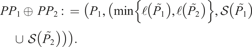
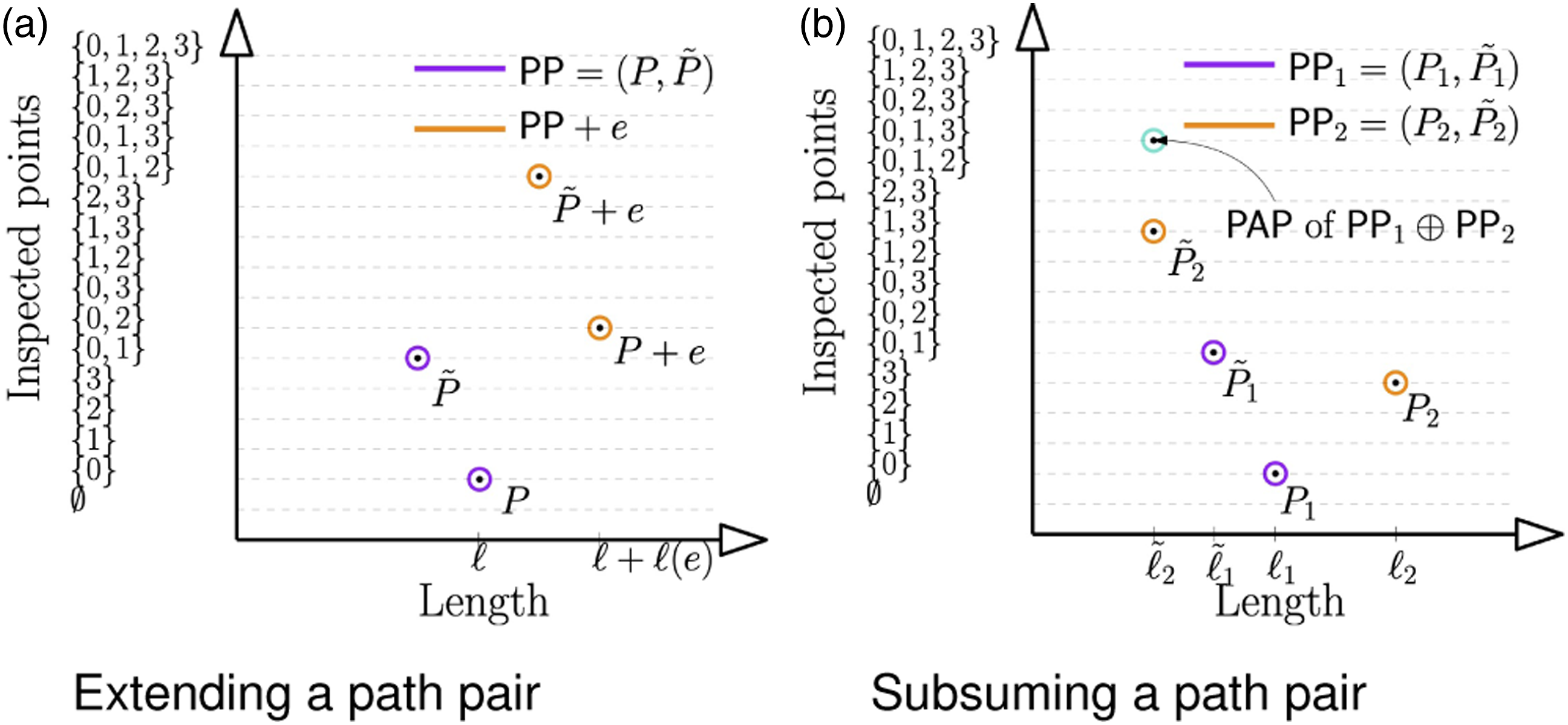
Depiction of operations on path pairs. (a) PP extended by an edge e = (u, v) with $\mathcal{S}\left(v\right)=\left\{2\right\}$ . (b) PP₁ subsuming PP₂. Note that P₁ is the achievable path of PP₁⊕PP₂ thus only the potentially achievable path is explicitly marked.

Definition 5. ɛ, p-bounded. A path pair $\mathsf{P}\mathsf{P}:=\left(P,\stackrel{\sim }{P}\right)$ is said to be ɛ, p-bounded for some ɛ ≥ 0 and p∈(0,1] if P ɛ, p-dominates $\stackrel{\sim }{P}$ .

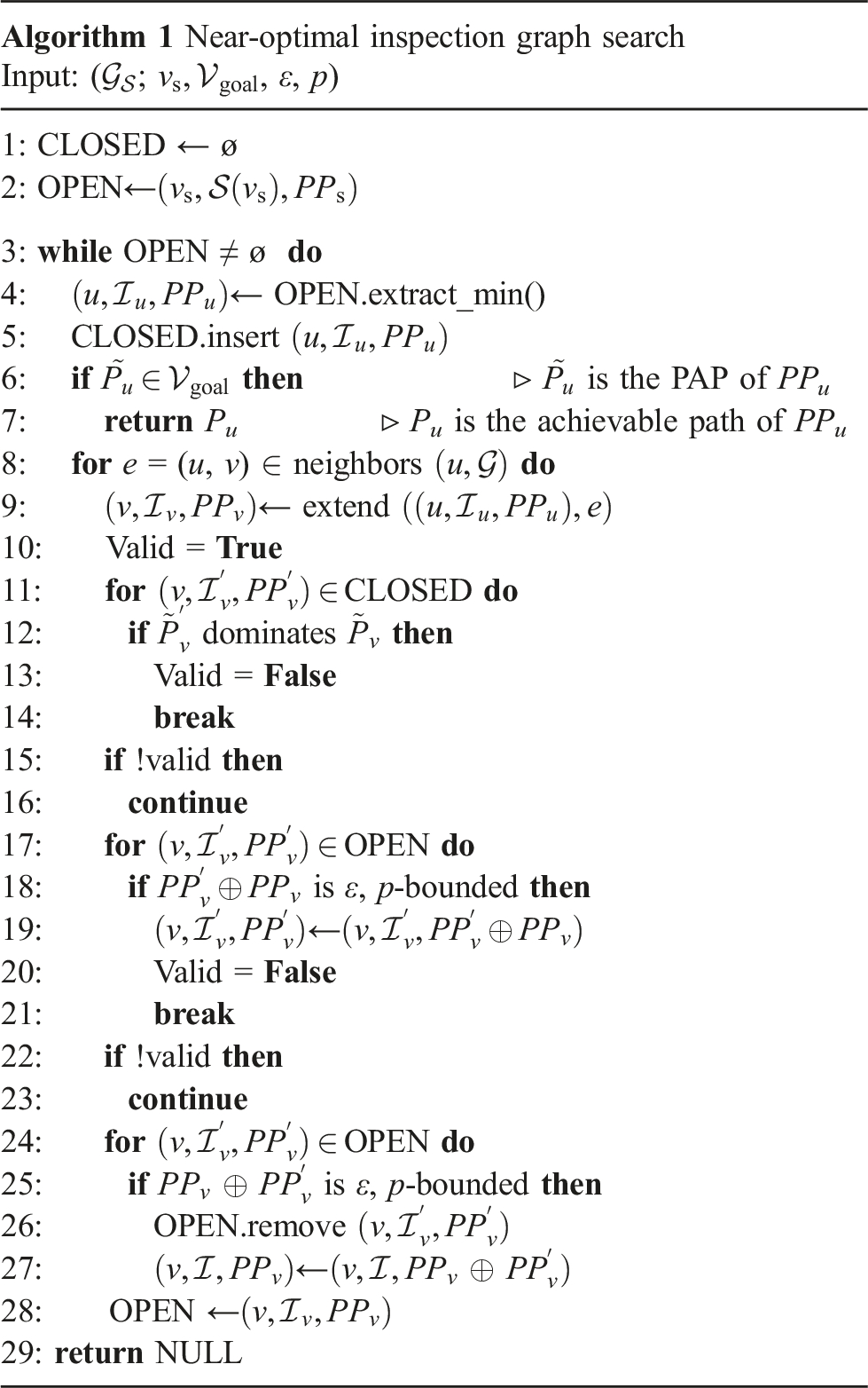
To compute a near-optimal inspection path (Alg. 1 and Figure 6), we extend each path considered by our search algorithm to be a path pair and use this additional data to prune away approximately dominated paths. Similar to A*, our algorithm uses two priority queues OPEN and CLOSED to track the nodes considered by the search. It starts by inserting the start vertex $\left(v_{\mathrm{s}},\mathcal{S}\left(v_{\mathrm{s}}\right)\right)$ to the OPEN list together with the path pair ${\mathsf{P}\mathsf{P}}_s=\left(P_{\mathrm{s}},P_{\mathrm{s}}\right)$ (here P_s is a path containing only start vertex v_s) (line 2).

Our algorithm proceeds in a similar fashion to A*—we pop the most promising node $n=\left(u,{\mathcal{I}}_u,{PP}_u\right)$ from OPEN (line 4) and move it to CLOSED (line 5). If the PAP of this node is in the goal set ${\mathcal{V}}_{\text{goal}}$ (line 6), we terminate the search and return the achievable path of PP _u (line 7). If not, we consider all neighboring edges e of u in $\mathcal{G}$ and extend the node n (line 9). This is akin to computing n’s neighbors in ${\mathcal{G}}_{\mathcal{S}}$ .

At this point, our algorithm deviates from the standard A* algorithm. For each newly created node $\left(v,{\mathcal{I}}_v,{\mathsf{P}\mathsf{P}}_v\right)$ we check if there exists a node in CLOSED whose PAP dominates ${\stackrel{\sim }{P}}_v$ . If so, this node is discarded (lines 11–14). If no such node exists in the CLOSED list, we check if there exists a node in OPEN that may subsume it. If so, that node is updated and this node is discarded (line 17–21). Finally, we check if this node can subsume nodes that are in OPEN. If so, such nodes are discarded and this node is updated. (line 24–27).

We prove that, Alg. 1 returns a path that ɛ, p-dominates an optimal inspection path on the roadmap (see Sec. 6).

Figure 6.

Visualization of Alg. 1 initialized with ɛ = 2/3 and p = 1/2 (only the relevant parts of the inspection graph are depicted). (a, ) with the trivial PAP of length zero and no points inspected. (a) Two paths (red and blue) are extended from the start node to (b, {0}) and (c, {1}) with path pairs PP₁ and PP₂, respectively (the PAPs of each path have the same length and coverage as the paths themselves). (b) Blue path extended to (d, {0}) with $\mathit{\ell }\left(P_1\right)=\mathit{\ell }\left(\stackrel{\sim }{P_1}\right)=2$ and $\mathcal{S}\left(P_1\right)=S\left(\stackrel{\sim }{P_1}\right)=\left\{0\right\}$ . (c) Red path extended to (d, {1}) with $\mathit{\ell }\left(P_2\right)=\mathit{\ell }\left(\stackrel{\sim }{P_2}\right)=3$ and $\mathcal{S}\left(P_2\right)=S\left(\stackrel{\sim }{P_2}\right)=\left\{1\right\}$ . Here, PP₁⊕PP₂ ε,p-dominates PP₂ and the red path is discarded and PAP₁ is updated to have length two and coverage {0, 1} (d) Blue path extended to vertex (e, {0, 2}). Here, $\mathit{\ell }\left(P_1\right)=\mathit{\ell }\left(\stackrel{\sim }{P_1}\right)=3$ and $\mathcal{S}\left(P_1\right)=\left\{\mathrm{0,2}\right\},S\left(\stackrel{\sim }{P_1}\right)=\left\{\mathrm{0,1,2}\right\}$ . The algorithm terminates with the path a − b − d − e whose length is 3 and has coverage of {0, 2}. Notice that the path a − c − d − e (not computed) is optimal as its length is four and it has complete coverage. The computed path is within the bounds ensured by the approximation factor p and ɛ.

5.3. Tightening approximation factors

Recall that our algorithm starts with approximation parameters p₀ and ɛ₀. We endow our algorithm with a tightening factor f ∈ (0,1], and at the i’th iteration we set our approximation parameters as p _i = p_i−1 + f ⋅ (1 − p_i−1) and ɛ _i = ɛ_i−1 + f ⋅ (0 − ɛ_i−1). As we will see (Sec. 6), since $\underset{N\to \infty }{\lim }$ p _i = 1, $\underset{N\to \infty }{\lim }$ ɛ _i = 0, the tightening allows our method to achieve asymptotic optimality.

Algorithm 1 Near-optimal inspection graph search Input: ( ${\mathcal{G}}_{\mathcal{S}}$ ; $v_{\mathrm{s}},{\mathcal{V}}_{\text{goal}}$ , ɛ, p)
1: CLOSED ← ø
2: $\text{OPEN}\leftarrow \left(v_{\mathrm{s}},\mathcal{S}\left(v_{\mathrm{s}}\right),{\mathsf{P}\mathsf{P}}_{\mathrm{s}}\right)$
3: while OPEN ≠ ø do
4:   $\left(u,{\mathcal{I}}_u,{\mathsf{P}\mathsf{P}}_u\right)\leftarrow$ OPEN.extract_min()
5:  CLOSED.insert $\left(u,{\mathcal{I}}_u,{\mathsf{P}\mathsf{P}}_u\right)$
6:  if $\stackrel{\sim }{P_u}\in {\mathcal{V}}_{\text{goal}}$ then       ⊳ $\stackrel{\sim }{P_u}$ is the PAP of PP u
7:   return P u     ⊳ P u is the achievable path of PP u
8:  for e = (u, v) ∈ neighbors $\left(u,\mathcal{G}\right)$ do
9:    $\left(v,{\mathcal{I}}_v,{\mathsf{P}\mathsf{P}}_v\right)\leftarrow$ extend $\left(\left(u,{\mathcal{I}}_u,{\mathsf{P}\mathsf{P}}_u\right),e\right)$
10:   Valid = True
11:   for $\left(v,{\mathcal{I}}_v^{\prime },{\mathsf{P}\mathsf{P}}_v^{\prime }\right)\in \text{CLOSED}$ do
12: if ${\stackrel{\sim }{P}}_v^{\prime }$ dominates ${\stackrel{\sim }{P}}_v$ then
13: Valid = False
14: break
15: if !valid then
16: continue
17: for $\left(v,{\mathcal{I}}_v^{\prime },{\mathsf{P}\mathsf{P}}_v^{\prime }\right)\in \text{OPEN}$ do
18: if ${\mathsf{P}\mathsf{P}}_v^{\prime }\oplus {\mathsf{P}\mathsf{P}}_v$ is ɛ, p-bounded then
19: $\left(v,{\mathcal{I}}_v^{\prime },{\mathsf{P}\mathsf{P}}_v^{\prime }\right)\leftarrow \left(v,{\mathcal{I}}_v^{\prime },{\mathsf{P}\mathsf{P}}_v^{\prime }\oplus {\mathsf{P}\mathsf{P}}_v\right)$
20: Valid = False
21: break
22: if !valid then
23: continue
24: for $\left(v,{\mathcal{I}}_v^{\prime },{\mathsf{P}\mathsf{P}}_v^{\prime }\right)\in \text{OPEN}$ do
25: if ${\mathsf{P}\mathsf{P}}_v\oplus {\mathsf{P}\mathsf{P}}_v^{\prime }$ is ɛ, p-bounded then
26: OPEN.remove $\left(v,{\mathcal{I}}_v^{\prime },{\mathsf{P}\mathsf{P}}_v^{\prime }\right)$
27: $\left(v,\mathcal{I},{\mathsf{P}\mathsf{P}}_v\right)\leftarrow \left(v,\mathcal{I},{\mathsf{P}\mathsf{P}}_v\oplus {\mathsf{P}\mathsf{P}}_v^{\prime }\right)$
28: OPEN $\leftarrow \left(v,{\mathcal{I}}_v,{\mathsf{P}\mathsf{P}}_v\right)$
29: return NULL

5.4. Implementation details

5.4.1. Lazy computation in graph inspection planning

We run our search algorithm on $\mathcal{G}$ (Alg. 1) without checking if its edges are collision-free or not (recall that only the edges of $\mathcal{T}$ were explicitly checked for collision). Once a solution is found, we start checking edges one by one until the entire path was found to be collision-free or until one edge is found to be in collision, in which case we remove it from the edge set. This approach is common to speed up motion-planning algorithms when edges are expensive to evaluate (Dellin and Srinivasa 2016; Haghtalab et al., 2018).

5.4.2. Node extension in graph inspection planning

Any optimal inspection path can be decomposed into a sequence of vertices that improve the coverage of the path called milestones. It is straightforward to see that an optimal inspection path will (i) terminate at a milestone and (ii) connect a pair of milestones via a shortest path in $\mathcal{G}$ . Following this observation, instead of extending each path P from a vertex u by all outgoing edges in $\mathcal{G}$ (Alg. 1, line 8), we run a Dijkstra-like search from u and collect all first-met vertices that can be milestones.

5.4.3. Heuristic computation in graph inspection planning

Recall that A* orders nodes in the OPEN list according to their computed cost-to-come added to a heuristic estimate of their cost to reach the goal. The heuristic function that we use for vertex $\left(u,{\mathcal{I}}_u\right)$ is computed as follows: we run a Dijkstra search on $\mathcal{G}$ from u and consider the vertices ${\mathcal{V}}_u$ encountered during the search. We terminate when $\left({\cup }_{v\in {\mathcal{V}}_u}\mathcal{S}\left(v\right)\right)\hspace{0.17em}\cup \hspace{0.17em}{\mathcal{I}}_u={\mathcal{I}}_G$ and use the maximal distance between u to any node in ${\mathcal{V}}_u$ as our admissible (Hart et al., 1968) heuristic function. We now show why the heuristic is admissible. When we terminate with $\left({\cup }_{v\in {\mathcal{V}}_u}\mathcal{S}\left(v\right)\right)\hspace{0.17em}\cup \hspace{0.17em}{\mathcal{I}}_u={\mathcal{I}}_G$ , denote the last vertex added to ${\mathcal{V}}_u$ as v_last. Note that v_last is also the most distant (via roadmap edges) vertex from u due to the nature of Dijkstra’s algorithm. According to the termination condition, there exists a non-empty set of POI ${\mathcal{I}}_{\text{last}}$ that is covered by v_last but not covered by any other vertices in ${\mathcal{V}}_u$ . Namely, ${\mathcal{I}}_{\text{last}}\subset \mathcal{S}\left(v_{\text{last}}\right)$ and ${\mathcal{I}}_{\text{last}}\hspace{0.17em}\cap \hspace{0.17em}\left({\cup }_{v\in {\mathcal{V}}_u,v\ne v_{\text{last}}}\mathcal{S}\left(v\right)\right)=$ . To achieve an inspection coverage of ${\mathcal{I}}_{\mathcal{G}}$ , the minimum distance to travel is equal to or greater than the distance between u and v_last because with any shorter path, ${\mathcal{I}}_{\text{last}}$ is not covered.

6. Theoretical guarantees

In this section, we provide theoretical properties showing that IRIS is guaranteed to be asymptotically optimal, given that the system and the environment satisfy several general assumptions. For brevity, we only state the main definitions, lemmas, and theorems and defer all proofs to Appendix A and Appendix B. Recall that IRIS iteratively densifies the roadmap and runs a near-optimal inspection graph search on the latest roadmap. Thus, we begin (Thm. 1) by proving that our graph inspection search algorithm (Alg. 1) returns a near-optimal solution when compared to the optimal solution (available for that specific roadmap). We then continue (Thm. 2) to show that IRIS is asymptotically optimal when the approximation parameters satisfy that $\underset{N\to \infty }{\lim }$ ɛ _N = 0 and $\underset{N\to \infty }{\lim }$ p _N = 1, where N is the number of vertices in the roadmap. This is done by using the notion of probablistic exhaustivity (Schmerling et al., 2015) coupled together with the assumptions that (i) an optimal inspection trajectory is well behaved (Def. 8), (ii) an optimal inspection trajectory weak δ_cl-clearance, and that (iii) the inspection problem is regular (Def. 10). It is worth noting that all proofs are general enough to account for complex robotic systems, including those having differential constraints. Having said that, as we use a graph-based search method, we require a method is required to compute valid motions (if such motions exist) between two close-by configurations.

We start by proving that Alg. 1 is near-optimal.

Definition 6. Optimal inspection path on a roadmap. Let $\left(\mathcal{G},{\mathcal{I}}_{\mathcal{G}},\mathcal{S},\mathit{\ell },v_{\mathrm{s}}\right)$ be a graph inspection problem. An optimal inspection path P* is a path on roadmap $\mathcal{G}$ , starting at v_s, and satisfies

$\mathit{\ell }\left(P^{*}\right)=\mathrm{argmin}\left\{\mathit{\ell }\left(P\right)|P \text{is} \mathrm{a} \text{path} \text{with} \mathcal{S}\left(P\right)={\mathcal{I}}_{\mathcal{G}}\right\}.$

Where ℓ*≔ℓ(P*) and ${\mathcal{S}}^{*}:=\mathcal{S}\left(P^{*}\right)={\mathcal{I}}_{\mathcal{G}}$ , denote the length and coverage of an optimal path, respectively.

Lemma 1. In Alg. 1 (near-optimal inspection graph search), all path pairs in OPEN and CLOSED during the search are ɛ, p-bounded.

Lemma 2. Let $P^{*}=\left\{v_0,v_1,\dots ,v_{n^{*}}\right\}$ be an optimal inspection path and denote P*[i]≔{v₀, …, v _i }, for i ∈ [0, n*] as the path composed of the first i waypoints of P*. During every iteration of Alg. 1, there exists a path pair ${\mathsf{P}\mathsf{P}}_v=\left(P_v,{\stackrel{\sim }{P}}_v\right)$ in OPEN and an index i such that v = v _i and ${\stackrel{\sim }{P}}_v$ strictly dominates P*[i]. Namely, $\mathit{\ell }\left(\stackrel{\sim }{P}\right)\le \mathit{\ell }\left(P^{*}\left[i\right]\right)$ and $\left(P^{*}\left[i\right]\right)\subseteq \mathcal{S}\left(\stackrel{\sim }{P}\right)$ .

With Lemma 1 and 2, we can show that Alg. 1 returns a near-optimal result.

Theorem 1. Near-optimal inspection graph search. Near-optimal inspection graph search (Alg. 1) computes a path P that ɛ, p-dominates an optimal inspection path P*. Namely, ℓ(P) ≤ (1 + ɛ) ⋅ ℓ(P*) and $\left|\mathcal{S}\left(P\right)\right|\ge p·\left|\mathcal{S}\left(P^{*}\right)\right|$ .

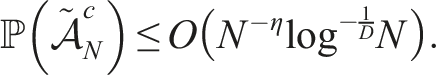
We now continue to prove that IRIS is asymptotically optimal. To prove this, we show that an optimal inspection path x* can be approximated by a sequence of configurations sampled by IRIS, given certain conditions. Specifically, we will need to show that as the number of iterations approaches infinity, the following requirements hold: (i) the length of the path induced by this sequence of samples converges asymptotically to the length of x*, (ii) the coverage obtained by this sequence of samples converges asymptotically to the coverage of x*, and that (iii) our inspection graph search algorithm finds such a sequence of samples. To do so, we rely on the notion of probabilistic exhaustivity (Schmerling et al., 2015). Roughly speaking, it is the notion that given a sufficiently large set of uniformly sampled configurations, any path can be traced arbitrarily well in the configuration space by a path defined as a sequence of configurations.

Lemma 3. Probabilistic exhausitivity. Let $x:\left[0,T\right]\to {\mathcal{X}}_{\text{free}}$ be a dynamically feasible trajectory. Let ${\mathcal{Q}}_N$ be a set of N points sampled independently and identically from the uniform distribution on the collision-free space ${\mathcal{X}}_{\text{free}}$ and set $V_N=\left\{x\left(0\right)\right\}\cup {\mathcal{Q}}_N$ .For a given N, set

$r_N=\kappa ·{\left(\log \left(N\right)/N\right)}^{1/D}.$

Here, D is a constant capturing the dimension of the system and κ is a commutable constant depending on the system dynamics, N, D, and some tuning parameter η ≥ 0. Let ${\stackrel{\sim }{\mathcal{A}}}_N$ be the event that there exists a discrete sequence of configurations $P={\left\{{\mathbf{q}}_i\right\}}_{i=1}^n\subseteq V_N$ that (δ, r)-traces x for any δ ∈ (0, 1) and r = r _N . The probability that event ${\stackrel{\sim }{\mathcal{A}}}_N$ doesn’t happen, denoted by $\mathbb{P}\left({\stackrel{\sim }{\mathcal{A}}}_N^c\right)$ is asymptotically bounded by

$\mathbb{P}\left({\stackrel{\sim }{\mathcal{A}}}_N^c\right)\le O\left(N^{-\eta }{\log }^{-\frac{1}{D}}N\right).$

As is defined above, η ≥ 0 is some tuning parameter.

In addition, we assume that x* is well-behaved. Roughly speaking, this ensures that there are no singular points along the trajectory where a POI can only be inspected from. This, in turn, will allow us to ensure that trajectories that trace an optimal inspection path cover the same set of POI.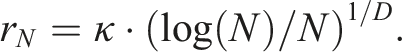

Definition 7. Inspecting configuration region. Let $i\in \mathcal{I}$ be a point of interest (POI), the inspecting configuration region of i, denoted as ${\mathcal{X}}_{\text{insp}}\left(i\right)$ , is defined to be the union of all configurations from which the POI can be inspected. Namely,

${\mathcal{X}}_{\text{insp}}\left(i\right)=\left\{\mathbf{q}\in {\mathcal{X}}_{\text{free}}:i\in \mathcal{S}\left(\mathbf{q}\right)\right\}.$

Similarly, the inspecting configuration region of ${\mathcal{I}}^{\prime }\subseteq \mathcal{I}$ is defined as

${\mathcal{X}}_{\text{insp}}\left({\mathcal{I}}^{\prime }\right)=\left\{\mathbf{q}\in {\mathcal{X}}_{\text{free}}:{\mathcal{I}}^{\prime }\subseteq \mathcal{S}\left(\mathbf{q}\right)\right\}.$

Definition 8. Well-behaving of an inspection trajectory. Let $x:\left[0,T\right]\to {\mathcal{X}}_{\text{free}}$ be a feasible inspection trajectory. x is said to be strongly ξ-well behaved if $\forall i\in \mathcal{S}\left(x\right)$ , there exist at least one point along x whose ξ-neighborhood is completely within the inspecting configuration region of i. Namely,

$\forall i\in \mathcal{S}\left(x\right),\exists t\in \left[0,T\right] \mathrm{s}.\mathrm{t}. B^e\left(x\left(t\right),\xi \right)\subseteq {\mathcal{X}}_{\text{insp}}\left(i\right).$

Similarly, x is said to be weakly ξ-well behaved if $\forall i\in \mathcal{S}\left(x\right)/\left(\mathcal{S}\left(x\left(0\right)\right)\cup \mathcal{S}\left(x\left(T\right)\right)\right)$ , there exists at least one point along x whose ξ-neighborhood is completely within the inspecting configuration region of i. Namely

$\begin{array}{l}\forall i\in \mathcal{S}\left(x\right)/\left(\mathcal{S}\left(x\left(0\right)\right)\hspace{0.17em}\cup \hspace{0.17em}\mathcal{S}\left(x\left(T\right)\right)\right),\exists t\in \left[0,T\right]\\ \mathrm{s}.\mathrm{t}. B^e\left(x\left(t\right),\xi \right)\subseteq {\mathcal{X}}_{\text{insp}}\left(i\right).\end{array}$

It is not hard to see, that any strongly well-behaved trajectory can be shortened to a weakly well-behaved trajectory without loosing coverage. Thus an optimal inspection trajectory can only be weakly well-behaved.

We further require the inspection-planning problem to be regular. The notion of regularity is required because for a weakly well-behaved optimal inspection trajectory $x*:\left[0,T\right]\to {\mathcal{X}}_{\text{free}}$ we need to take special care to cover the POI inspected at x*(T). The notion of regularity will ensure that there always exists a region near x*(T) that IRIS can sample inside.

Definition 9. Regular boundary. A set ${\mathcal{X}}^{\prime }\subseteq {\mathcal{X}}_{\text{free}}$ is said to have a regular boundary if there exists γ > 0 such that $\forall \mathbf{q}\in \partial \mathcal{X}$ , there exists $\mathbf{q}\prime \in \mathcal{X}$ with $B^e\left(\mathbf{q}\prime ,\gamma \right)\subseteq {\mathcal{X}}^{\prime }$ and q ∈ ∂B ^e (q′, γ).

Definition 10. Regularity of an inspection-planning problem. Let $\mathcal{P}=\left(\mathcal{X},\mathcal{I},\mathcal{S},\mathcal{\ell },q_{\mathrm{s}}\right)$ be an inspection-planning problem and ${\mathcal{X}}_{\text{free}}$ be the set of collision-free configurations. $\mathcal{P}$ is said to be regular if $\forall \mathbf{q}\in {\mathcal{X}}_{\text{free}}$ , ${\mathcal{X}}_{\text{insp}}\left(\mathcal{S}\left(\mathbf{q}\right)\right)$ has a regular boundary.

Similar to many other analyses of sampling-based planning algorithms (see, e.g., Kavraki et al. (1996); Karaman and Frazzoli (2011); Solovey et al. (2018)), we also assume that an optimal trajectory to trace has clearance from ${\mathcal{X}}_{\text{obs}}$ .

Definition 11. Strong/weak δ_cl-clearance. Let $x:\left[0,T\right]\to {\mathcal{X}}_{\text{free}}$ be a feasible trajectory. x has strong δ_cl -clearance if ∀t ∈ [0, T], x(t) is in δ_cl -interior of ${\mathcal{X}}_{\text{free}}$ (namely, x(t) is at least δ_cl away from any point in ${\mathcal{X}}_{\text{obs}}$ using the Euclidean distance). Furthermore, x has weak δ_cl -clearance if there exists a sequence of homotopic paths ${\left\{x_k\right\}}_{k\in \mathbb{N}}$ that satisfies:

(i) $\underset{k\to \infty }{\lim }$ x _k = x.

(ii) x₀ has strong δ_cl-clearance.

(iii) ∀k∈[0,∞), x _k is dynamically feasible and has strong δ _k -clearance for some δ _k > 0, and $\underset{k\to \infty }{\lim }$ δ _k = 0.

(iv) $\underset{k\to \infty }{\lim }$ ℓ(x _k ) = ℓ(x).

We are finally ready to state our final theorem.

Theorem 2. IRIS asymptotic optimality. Let $\mathcal{P}=\left(\mathcal{X},\mathcal{I},\mathcal{S},\mathit{\ell },{\mathbf{q}}_s\right)$ be a regular inspection-planning problem and ${\mathcal{X}}_{\text{free}}$ be the collision-free space. Assume that the robot system satisfies the assumptions mentioned in Schmerling et al. (2015) and Let $x^{*}:\left[0,T\right]\to {\mathcal{X}}_{\text{free}}$ be an optimal feasible inspection trajectory such that

(i) x*(0) = q _s ,

(ii) x* has weak δ_cl-clearance for some δ_cl > 0,

(iii) x* is weakly ξ-well behaved for some ξ > 0.

Furthermore, let ℓ _i and ${\mathcal{S}}_i$ denote the arc length, and the inspection coverage, respectively of the trajectory returned by IRIS at the N’th iteration using approximation parameters ɛ _N and p _N , and a lower-bound connecting radius r _N (as defined in Lemma 4). If $\underset{N\to \infty }{\lim }$ ɛ _N = 0 and $\underset{N\to \infty }{\lim }$ p _N = 1, we have that

$\underset{N\to \infty }{\lim }\mathbb{P}\left({\mathit{\ell }}_N>\left(1+\mathrm{\Delta }\right)\mathit{\ell }\left(x^{*}\right)\right)=0$

for any Δ >0 and that

$\underset{N\to \infty }{\lim }\mathbb{P}\left(\left|{\mathcal{S}}_N\right|<\left|{\mathcal{I}}^{*}\right|\right)=0.$

7. Results

We evaluated IRIS on three simulated scenarios: (1) a planar manipulator inspecting the boundary of a square region (Figure 7(a)), (2) an unmanned aerial vehicle (UAV) inspecting the outer surface of a bridge (Figure 7(b)), and (3) a CRISP robot inspecting the inner surface of a pleural cavity (Figure 7(c)). For all experiments, we order path pairs in OPEN (Alg. 1 line 4) according to the path pair with the minimal potentially achievable path cost. All tests were run on a 3.4 GHz 8-core Intel Xeon E5-1680 CPU with 64 GB of RAM.

Figure 7.

Simulation scenarios. (a) A 5-link planar manipulator (orange) inspects the boundary of a square region (blue) where rectangular obstacles (red) may block the robot and occlude the sensor. The sensor’s field of view (FOV) is represented by the yellow region. 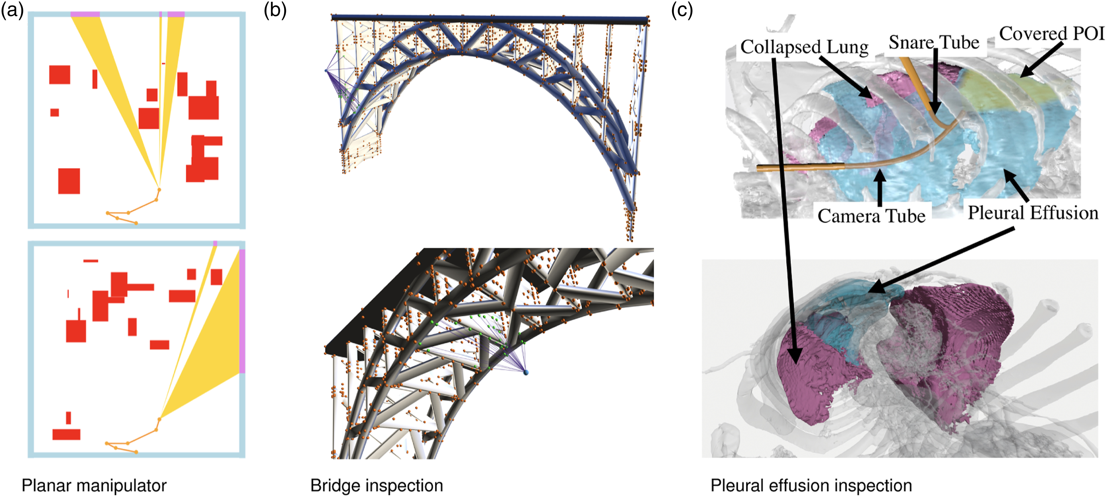$\mathcal{S}\left(\mathbf{q}\right)$ are the points on the boundary in the sensor’s unobstructed FOV and are shown in purple. (b) The bridge inspection scenario involves a UAV (blue) inspecting the outer surface of a bridge, including the POI that are covered (green) and non-covered (orange) from the current configuration. (c) The pleural effusion inspection scenario involves the CRISP robot (orange) inspecting the inner surface of a pleural cavity, including the POI that are covered (green) and non-covered (blue) from the current robot configuration.

7.1. Planar manipulator scenario

In this scenario, depicted in Figure 7(a), we have a 5-link planar manipulator fixed at its base that is tasked with inspecting the boundary of a rectangular 2D workspace, which is discretized into 400 POI. The sensor is a camera attached to the tip of the manipulator, aligning with the direction of the robot’s final segment. When modeling the camera for inspection, we consider a field of view (FOV) of 45° and an unbounded effective inspecting distance. We start by evaluating IRIS for fixed p and ɛ and then compare it with RRTOT using our approach for dynamically reducing the approximation factors. For every set of parameters, we ran 10 experiments for 1000 s and report the average value together with the standard deviation.

This scenario serves as a simple example where we compare the approximation algorithm for inspection planning with optimal inspection planning (i.e., p = 1, ɛ = 0). When p = 1, indicating we do not allow any approximation on inspection coverage, and we vary ɛ (Figure 8(a)), we can see that even small approximation factors (e.g., ɛ = 0.5) allow to dramatically increase the coverage obtained as each search episode takes less time and more configurations can be added to the RRT tree. While optimal inspection planning (using ɛ = 0) did not result in 80% coverage even after 1000 s, this was achieved within one second for ɛ ≥ 1.0. This comes at the price of slightly longer inspection paths. When ɛ = 0, indicating we do not allow any approximation on path length, and we vary p (Figure 8(b)), we get roughly the same coverage per time but at the price of much longer paths for higher values of p.

Figure 8.

Quality of inspection paths computed for the planar manipulator. The algorithm falls back to optimal inspection planning when p = 1, ɛ = 0. (a) IRIS running with p = 1, f = 0 and varying values of ɛ. (b) IRIS running with ɛ = 0, f = 0 and varying values of p. (c) Comparison of IRIS and RRTOT. IRIS running with p₀ = 0.95, ɛ₀ = 20.0, and f = 0.0005.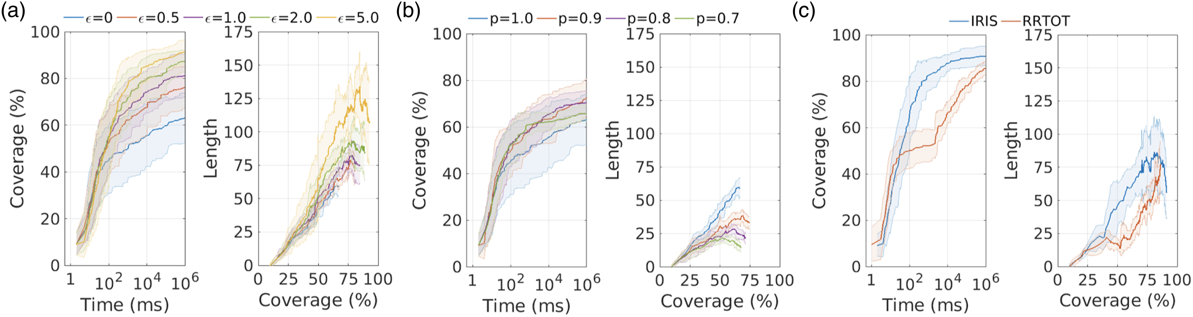

Following the above discussion, when reaching high coverage is the sole objective, one should use large initial values of p₀ and ɛ₀. When we want initial solutions to also be short, one should start with smaller approximation factors. We compared IRIS with different initial approximation factors to RRTOT (Bircher et al., 2017), see Figure 8(c). We can see that our approach allows producing higher-quality paths than RRTOT. For example, IRIS obtains more than a 264× speedup when compared to RRTOT when producing the same quality of inspection planning for the case of roughly 85% coverage and path length of 85.8 units. Final inspection paths obtained by IRIS are both shorter and inspect larger portions of $\mathcal{I}$ .

7.2. Bridge inspection scenario

In this scenario, depicted in Figures 7(b) and (a) UAV equipped with a camera inspects the surface of a bridge structure. The bridge structure is obtained from a 3D mesh (Elkassar 2008) and discretized into 3817 POI. The bridge structure serves as both an inspection target and an obstacle that may block movements and occlude sensing. And we do not consider other environmental obstacles except for the ground, which means the UAV can only fly above the ground.

The UAV has a configuration space of $\mathcal{S}\mathcal{O}\left(2\right)\times {\mathbb{R}}^3$ . It first can translate in 3D space, then can rotate around its vertical axis, and finally, the camera can rotate around the pitch axis. When modeling the camera for inspection, we consider a FOV of 90° and an effective inspecting distance of 10 m.

We ran IRIS and RRTOT for this scenario 10 different times for 10,000 s (Figure 9). IRIS obtains more than a 8× speedup when compared to RRTOT when producing a better quality of inspection planning for the case of roughly 57% coverage and path length of 230 units, which is only 68% of that of RRTOT.

Figure 9.

Comparing the quality of inspection paths computed for the bridge inspection scenario. IRIS was run with p₀ = 0.7, ɛ₀ = 5, and f = 0.0001.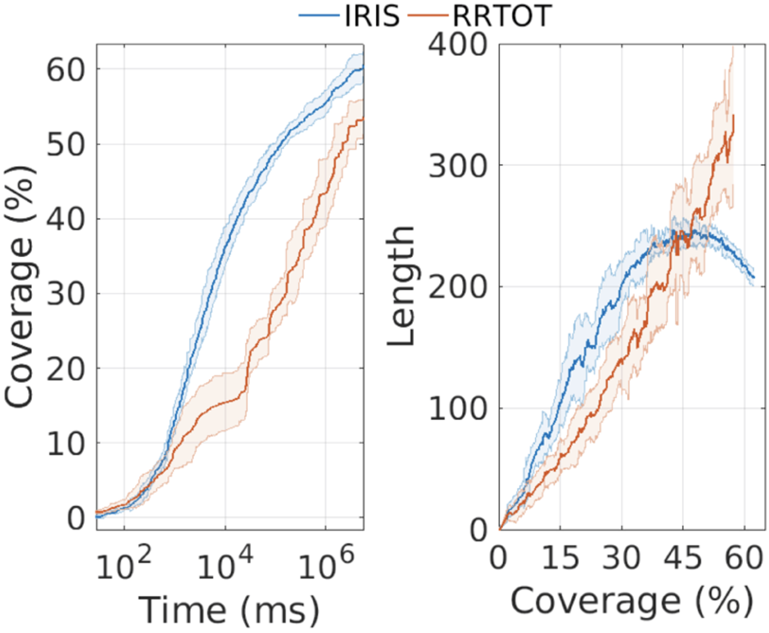

7.3. Pleural effusion inspection scenario

The anatomical pleural effusion environment for this simulation scenario was obtained from a Computed Tomography (CT) scan of a real patient suffering from this condition, and a fine discretization of the internal surface of the pleural cavity is used as the set of POI containing 49506 points. We also use the internal surface of the cavity as obstacles and prohibit the robot from colliding with the pleural surface, lung, and chest wall (except at tube entry points). Pleural effusion volumes can be geometrically complex, as the way in which the lung separates from the chest wall can be inconsistent. This results in unseparated regions of the lung’s surface that can inhibit movement and occlude the sensor from visualizing areas further in the volume.

Here we consider a CRISP robot with two tubes, where a snare tube is grasping a camera tube in order to create a parallel structure made of thin, flexible tubes. Each tube can be independently rotated in three dimensions about its entry point into the body, and independently translated into and out of the cavity. The system has 8 degrees of freedom with a configuration space of $\mathcal{S}\mathcal{O}{\left(3\right)}^2\times {\mathbb{R}}^2$ , which enables the parallel structure to move in a manner that enables obstacle avoidance as well as precise control of the camera’s pose. We model the camera with a 60-degree FOV and an unbounded effective inspecting distance.

We ran IRIS and RRTOT for this scenario 10 different times for 10,000 s (Figure 10). Similar to the planar manipulator scenario, IRIS allows producing higher-quality paths than RRTOT. For example, IRIS obtains more than a 79× speedup when compared to RRTOT when producing the same quality of inspection planning for the case of roughly 33% coverage and path length of 0.3 units.

Figure 10.

Comparing the quality of inspection paths computed for the pleural effusion scenario. IRIS was run with p₀ = 0.8, ɛ₀ = 10, and f = 0.01.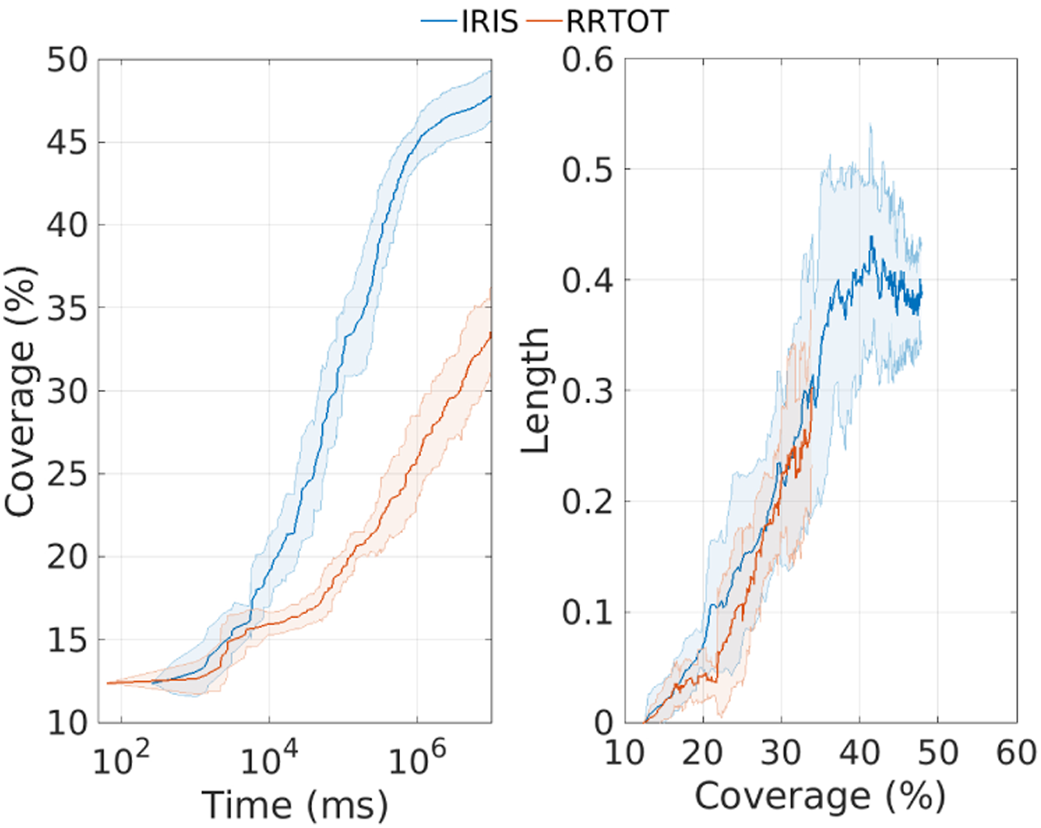

8. Conclusion and future work

In this work, we presented IRIS, an algorithmic framework for computing asymptotically optimal inspection plans. Our key contribution is an algorithm to efficiently compute near-optimal inspection plans on graphs. Interestingly, our problem of graph-inspection planning lies in the intersection between single and bi-criteria shortest path problems. Clearly, we are computing a shortest path on the inspection graph ${\mathcal{G}}_{\mathcal{S}}$ . However, en route, we compute an approximation of the set of Pareto-optimal paths to every node in the original graph $\mathcal{G}$ . Thus, we believe that our approach may be useful for the general problem of bicriteria optimization.

We showed IRIS outperforms the prior state-of-the-art, including in a medical application in which a surgical robot inspects a tissue surface inside the body as part of a diagnostic procedure. However, the efficiency of IRIS can be further improved. We now highlight several avenues where such improvement could be obtained.

8.1. Dynamic updates in graph inspection planning

IRIS reruns Alg. 1 every iteration which may be highly inefficient as we would like to reuse information constructed from previous search episodes. Indeed, the general case where a graph undergoes a series of edge insertions and edge deletions and we wish to update a shortest-path algorithm is a well-studied problem referred to as the fully dynamic single-source shortest-path problem (Frigioni et al., 2000; Ramalingam and Reps 1996). Efficient algorithms exist even when running an A*-like search (Koenig et al., 2004). Thus, an immediate next step to improve the efficiency of our algorithm is to adapt the aforementioned algorithms to the case of near-optimal graph inspection planning.

8.2. Balancing graph search and lazy computation

Recall that we employ a lazy search paradigm when computing near-optimal inspection plans on the inspection graph (Sec. 5.4). This was done because edge evaluation is computationally complex. However, as the number of iterations increases, the search starts to dominate the overall running time of our algorithm and not edge evaluation (see Figure 11). Recently Mandalika et al. (2018, 2019) presented an algorithm that balances edge evaluation and graph search when edges are expensive to evaluate using the notion of lazy look-ahead. Thus, we suggest using their method dynamically varying the so-called lazy look-ahead—in the initial stages of the algorithm, when the search is not a bottleneck, employ a large look-ahead (which corresponds to performing more search). As the algorithm progress, reduce the look-ahead to account for the fact that edge evaluation is relatively cheaper than graph search.

Figure 11.

Time decomposition of IRIS as a function of iteration number.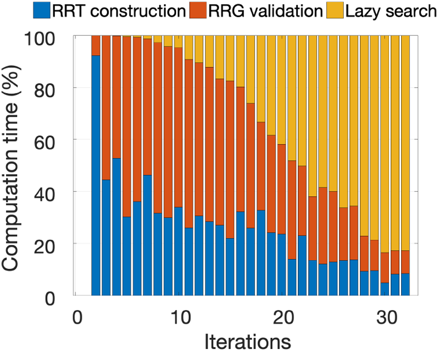

8.3. Efficient sampling of configurations in RRT construction

Recall that in our RRT constructions we sample configurations uniformly at random from $\mathcal{X}$ . Common implementations of RRT typically employ a goal bias where configurations from the goal are sampled with some probability LaValle (2006). Similarly, we suggest biasing sampling towards configurations that increase coverage. Namely, to configurations q such that $\mathcal{S}\left(\mathbf{q}\right)\cup {\mathcal{I}}_G\ne$ . We suspect that the goal bias should be dynamically changed—when the inspection graph ${\mathcal{G}}_{\mathcal{S}}$ has low coverage the bias should be high. As the overall coverage of ${\mathcal{G}}_{\mathcal{S}}$ increases, the goal bias should be reduced to allow for shorter inspection plans.

8.4. Employing multiple heuristics in graph inspection planning

As the number of iterations increases, graph search dominates the running time of our algorithm. Heuristics have been shown to be an effective tool in speeding up search algorithms and we suggest employing recent developments from the search community to speed up this part of our framework. One such development is using multiple heuristics to guide the search in a systematic way (Aine et al., 2016) that has shown to be an effective tool in robot planning algorithms (Islam et al., 2018; Ranganeni et al., 2018).

Roughly speaking, using multiple heuristics allows encoding domain knowledge without having to worry about the heuristic functions being admissible. In our setting, we are simultaneously reasoning about inspection coverage and plan length in our graph inspection planning. Thus, it may be beneficial to design one (or more) heuristics that account for path length and one (or more) heuristics that account for path coverage. Then we could apply a method similar to MHA* (Aine et al., 2016) to combine the efforts of these heuristics.

8.5. Adaptively updating approximation parameters

In our work, we used a simplistic approach to update the approximation parameters. These may have a dramatic effect on the quality of plans produced. We suggest further inspecting how to update these parameters, possibly doing this in a dynamic fashion according to information obtained from previous search episodes.