Sage Journals: Discover world-class research

Abstract

Recent advances in deep learning technology have triggered radical progress in the autonomy of ground vehicles. Marine coastal Autonomous Surface Vehicles (ASVs) that are regularly used for surveillance, monitoring, and other routine tasks can benefit from this autonomy. Long haul deep sea transportation activities are additional opportunities. These two use cases present very different terrains—the first being coastal waters—with many obstacles, structures, and human presence while the latter is mostly devoid of such obstacles. Variations in environmental conditions are common to both terrains. Robust labeled datasets mapping such terrains are crucial in improving the situational awareness that can drive autonomy. However, there are only limited such maritime datasets available and these primarily consist of optical images. Although, long wave infrared (LWIR) is a strong complement to the optical spectrum that helps in extreme light conditions, a labeled public dataset with LWIR images does not currently exist. In this paper, we fill this gap by presenting a labeled dataset of over 2900 LWIR segmented images captured in coastal maritime environment over a period of 2 years. The images are labeled using instance segmentation and classified into seven categories—sky, water, obstacle, living obstacle, bridge, self, and background. We also evaluate this dataset across three deep learning architectures (UNet, PSPNet, DeepLabv3) and provide detailed analysis of its efficacy. While the dataset focuses on the coastal terrain, it can equally help deep sea use cases. Such terrain would have less traffic, and the classifier trained on cluttered environment would be able to handle sparse scenes effectively. We share this dataset with the research community with the hope that it spurs new scene understanding capabilities in the maritime environment.

Keywords

Autonomous surface vehicles long wave infrared instance segmentation object detection dataset

1. Introduction

In recent years, advances in deep learning algorithms have led to an exponential growth in the research on autonomy of land vehicles. Some of the key catalysts for this growth have been publicly available labeled datasets, open-source software, publication of novel deep learning architectures, and increase in hardware compute capabilities. The maritime environment, with an abundance of periodic tasks such as monitoring, surveillance, and long haul transportation presents a strong potential for autonomous navigation. Availability of good datasets is a key dependency for gaining autonomy. The challenge lies in interpreting this data and creating labeled datasets that can help train deep learning architectures.

Electro-Optical (EO) cameras are predominantly used to capture images because they are inexpensive and ubiquitous. In autonomous driving, sign posts, traffic lights, lane markings etc. can be easily recognized from a colored image. The abundance of Convolutional Neural Network (CNN) architectures by Krizhevsky et al. (2012) that learn from the labeled images has helped in making EO cameras mainstream. Two methods are commonly used for annotating an image. First, detecting objects of interest by drawing bounding boxes around them. Second, semantically segmenting an image in which each pixel is assigned a class label. The first method is faster as it focuses on specific targets; however, the second is more refined as it segments the entire scene.

The maritime environment is exposed to sky and water and the lighting conditions are therefore quite different as compared to a ground terrain. Glitter, reflection, water dynamism, and fog are common. These conditions deteriorate the quality of optical images. Horizon detection is also a common problem faced while using optical images. On the other hand, LWIR images offer distinct advantages in such extreme light conditions as shown experimentally by Robinette et al. (2019), Nirgudkar and Robinette (2021) and as shown in Figure 1. Marine robotics researchers have used LWIR sensors in their work (Schöller et al. (2019); Rodin and Johansen (2018); Qi et al. (2011); Wang et al. (2017)). Most notably Zhang et al. (2015) has built a labeled dataset of paired visible and LWIR images of different types of ships in the maritime environment. However, there are certain Figure 1 limitations of this dataset which are discussed in the next section.

Figure 1.

LWIR versus Optical cameras in extreme light conditions: In (a), sun’s glare is obstructing the view for optical while the visibility is clear in LWIR (b). In (c) visibility from optical camera is almost zero in the dark, whereas LWIR continues to give a clear picture (d).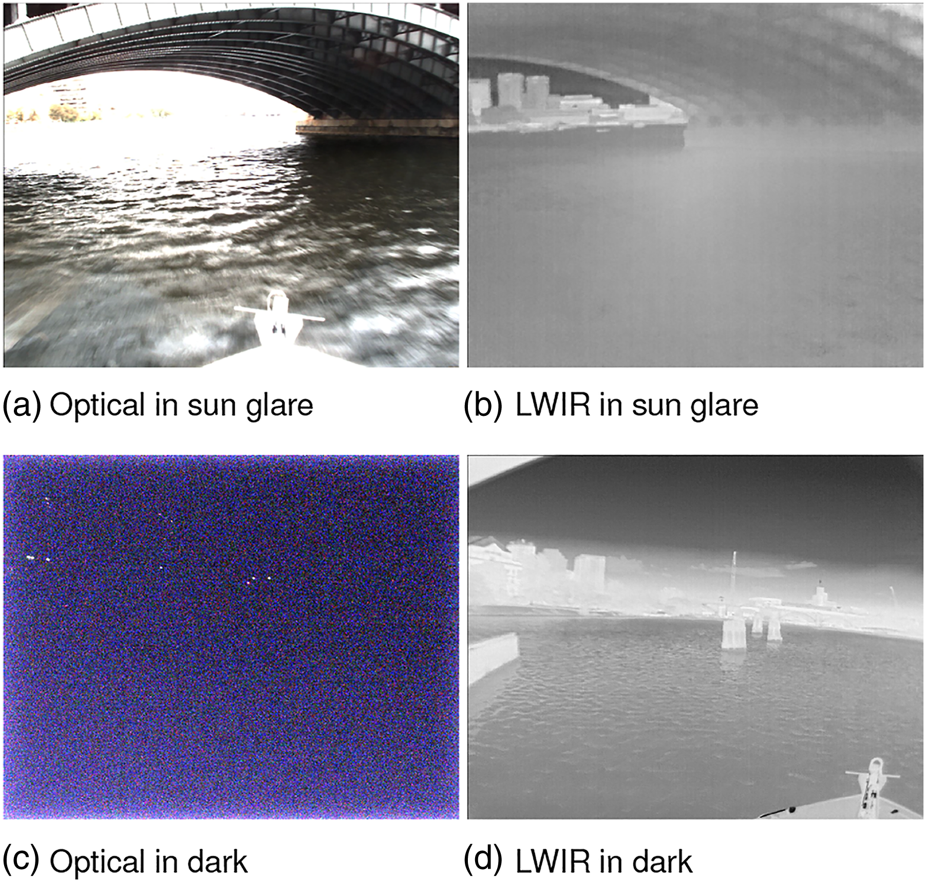

In this paper, we present a dataset of over 2900 LWIR maritime images that capture diverse scenes such as cluttered marine environment, construction, humans, marine wildlife, and nearshore views across various seasons and times of the day in the Massachusetts Bay area including Charles River and Boston Harbor. The dataset images are segmented using instance and semantic segmentation into 7 classes. We also evaluate the performance of this dataset across 3 popular deep learning architectures (UNet, PSPNet, DeepLabv3) and present our findings with respect to obstacle detection and scene understanding. The dataset is publicly available and can be downloaded from the URL ‘https://github.com/uml-marine-robotics/MassMIND’ Nirgudkar et al. (2022). We aim to stimulate research interest in the field of perception in maritime autonomy through this dataset.

The remainder of the paper has been organized as follows. Section 2 outlines the current state of art in the maritime domain. Section 3 describes the hardware assembly that is used for data acquisition. Specifics about the dataset and segmentation methods have been elaborated in Section 4 and Section 5 presents evaluation results against the 3 architectures. We draw conclusions in Section 6 and highlight the future plan of work.

2. Related work

Significant research has been carried out in the field of marine robotics over the past few years and researchers have developed multiple datasets that can aid autonomy. These datasets vary in size and complexity; however, their main purpose revolves around environment monitoring and surveillance. Castellini et al. (2020) used autonomous aquatic drones and captured multivariate time series data for the purpose of water quality management. The dataset contains parameters such as water conductivity, temperature, oxygen level and is useful for time series analysis. Bloisi et al. (2015) used ASV in Venice, Italy and created a dataset of optical images for the purpose of boat identification and classification. The ground truth in this dataset is provided in the form of bounding boxes. Images in this dataset contain close up view of boats. Each image is classified as one of the 24 categories of the boat. Ribeiro et al. (2019) captured images from an unmanned aerial vehicle (UAV) 150–300 m above ocean surface for research on sea monitoring and surveillance. Though multi-spectrum cameras including IR cameras are used, the dataset is not annotated and hence it cannot be used readily for model training. Another problem is that the images were aerial pictures and therefore do not have the same perception properties as that of the view from a vehicle on the water surface. Zhang et al. (2015) has created a dataset of paired visible and LWIR images of various ships in the maritime environment. The annotations are provided in the form of bounding boxes around ships. However, selection is focused on those images where ships occupy more than 200 pixels of the image area. The dataset is therefore not adaptable for general use where obstacles can be in any shape or form such as buoys, small platforms, and construction in water. More importantly, the images are captured from a static rig mounted on the shore and therefore lack the dynamism found in real-life scenarios.

Prasad et al. (2017) has created a dataset using optical and near infrared (NIR) cameras to capture maritime scenes from a stationary on-shore location. This dataset also has some video sequences recorded from a ship but they are from a higher vantage point and hence do not clearly depict the same view as that from an ASV. Additionally, not all images in the dataset are annotated. Only a few are annotated using bounding boxes. Patino et al. (2016) has used multi-spectrum cameras to capture video segments of enacted piracy scenes. The emphasis is on threat detection and so the video sequence contains medium to large boats appearing in the frames. Since the visuals are enforced, the dataset lacks natural marine scenes that are critical for training a model. Steccanella et al. (2020) used pixel wise segmentation to differentiate between water and non-water class. The dataset contains around 515 optical images with the 2 classes. In recent years, two excellent datasets MaSTR1325 and MODS have been created by Bovcon et al. (2019) and Bovcon et al. (2021). The optical images in these datasets are semantically segmented in 3 classes and are suitable for maritime scene understanding. However, as pointed out by Bovcon et al. (2021), bright sunlight, foam, glitter, and reflection in the water deteriorate the inference quality. Small object detection poses a challenge even for the model developed by Bovcon and Kristan (2020) that is specifically designed for the maritime environment.

The comparison of various marine datasets is shown in Table 1. Most of these datasets are captured using EO cameras. The ones that used NIR, do not provide the benefit of LWIR as they are still dependent on visible light. As indicated in Figure 2, Edmund Optics (2022) NIR light occupies a wavelength between 0.75 and 1.4 microns. Although it is a part of the infrared spectrum, it is not caused by thermal radiation. Instead, it is almost similar to visible light except that it cannot be observed by human eye. Heat or thermal radiation is the primary source of radiation for LWIR NASA (2003), Hyll (2016) and therefore LWIR is truly independent of visible light.

Table 1.

Publicly available dataset of images in maritime environment.

Name	Optical	IR	Bounding box	Semantic	Dynamic	Night	Labeled images	Resolution	Location
VAIS Zhang et al. (2015)	✓	✓	✓	✗	✗	✓ only IR	1000	EO:5056 × 5056 IR:1024 × 768	USA
SEAGULL Ribeiro et al. (2019)	✓	✓	✓	✗	✓	✗	Large¹	EO:1920 × 1080 IR:384 × 288	Portugal (UAV)
MarDCT Bloisi et al. (2015)	✓	✓	✓	✗	✗	✗	Large²	800 × 240	Italy
IPATCH Patino et al. (2016)	✓	✓	✗	✗	✓	✗	NA³	EO:1280 × 960	France
Singapore Maritime Dataset Prasad et al. (2017)	✓	✓ NIR	✓	✗	✓	✓ 2 h after dusk	High⁴	EO:1080 × 1920	Singapore
MaSTr1325 Bovcon et al. (2019)	✓	✗	✓*	✓ (3 classes)	✓	✗	1325	1278 × 958	Slovenia
IntCatch AI Castellini et al. (2020)	✓	✗	✗	✗	✓	✗	NA³	320 × 240 1920 × 1080 1280 × 720	Italy
MassMIND Nirgudkar et al. (2022)	✗	✓ LWIR	✓*	✓ (7 classes)	✓	✓	2900	640 × 512	USA

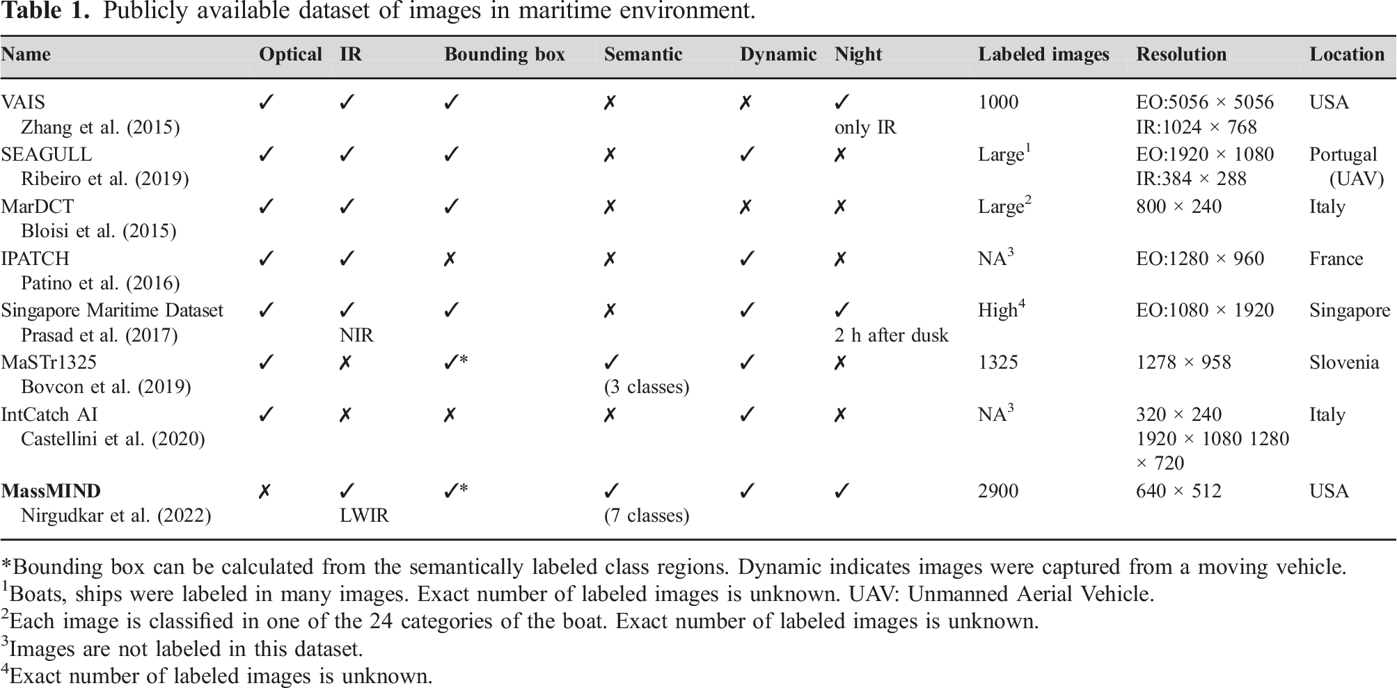
*Bounding box can be calculated from the semantically labeled class regions. Dynamic indicates images were captured from a moving vehicle.

¹Boats, ships were labeled in many images. Exact number of labeled images is unknown. UAV: Unmanned Aerial Vehicle.

²Each image is classified in one of the 24 categories of the boat. Exact number of labeled images is unknown.

³Images are not labeled in this dataset.

⁴Exact number of labeled images is unknown.

Figure 2.

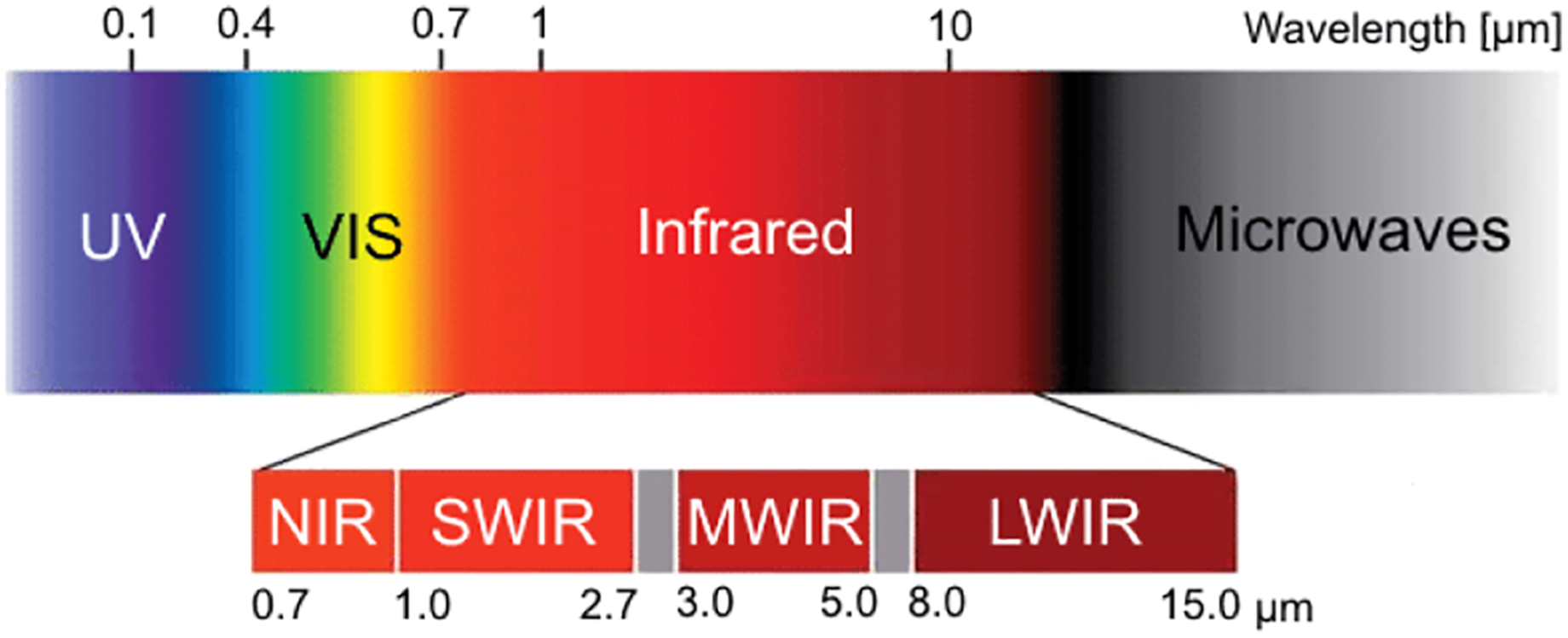
IR Spectrum.

In a nutshell, the existing NIR/LWIR datasets lack complete scene parsing capabilities, or have been created in a controlled environment or are not publicly available. MassMIND bridges this gap and is the largest labeled dataset of its kind containing real-life LWIR images. The images have been recorded in a busy marine area as well as in not so busy open waters during various seasons and times of the day over a period of 2 years. The dataset has been annotated into 7 classes using instance segmentation that can be used for scene parsing during autonomous navigation.

3. System setup

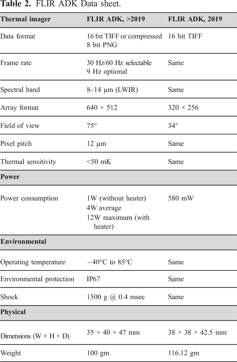
R/V Philos, an ASV owned by the Brunswick Corporation and operated by MIT Autonomous Underwater Vehicle (AUV) AUVLab (1989) lab was instrumental in collecting images for the MassMIND dataset. The ASV is equipped with 3 EO cameras, two Forward looking infrared (FLIR)-LWIR cameras, a radar, a lidar, GPS, and inertial measurement unit (IMU). The FLIR cameras used in 2019 were entry level providing resolution of 320 × 240 (width×height) and horizontal field of view of 34°. These cameras were upgraded in 2020 which provided resolution of 640 × 512 (width×height) and horizontal field of view of 75°. Images from these sensors have slight offset with one another due to the placement of EO and FLIR cameras as shown in Figure 3. Table 2 shows technical specifications of the FLIR ADK cameras used in the setup in 2019 and later. The vehicle was driven in and around Boston harbor by a human operator to collect the data and was not in autonomous mode most of the time. However, a limited autonomy for waypoint navigation and course holding was exercised. Additional details of the ASV can be found in DeFilippo et al. (2021). The unannotated raw dataset from the sensors was also released as part of that work SeaGrant (2022).

Figure 3.

R/V Philos showing placement of LWIR cameras.

Table 2.

FLIR ADK Data sheet.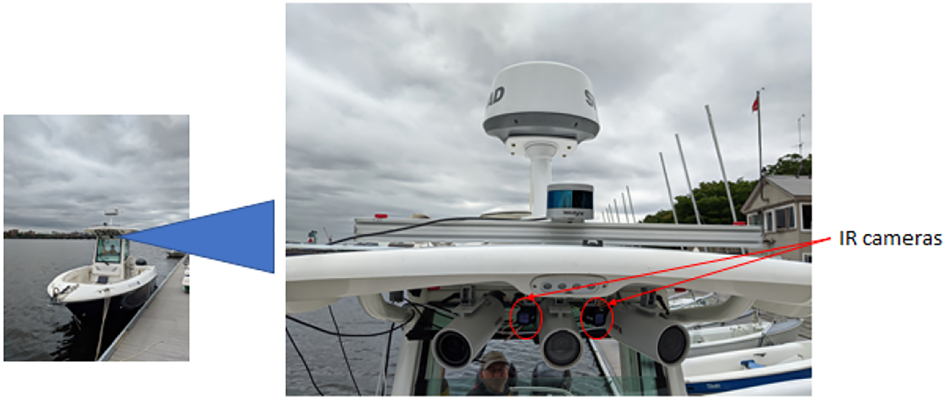

Thermal imager	FLIR ADK, >2019	FLIR ADK, 2019
Data format	16 bit TIFF or compressed	16 bit TIFF
Data format	8 bit PNG	16 bit TIFF
Frame rate	30 Hz/60 Hz selectable	Same
Frame rate	9 Hz optional	Same
Spectral band	8–14 μm (LWIR)	Same
Array format	640 × 512	320 × 256
Field of view	75°	34°
Pixel pitch	12 µm	Same
Thermal sensitivity	<50 mK	Same
Power
Power consumption	1W (without heater)	580 mW
	4W average
	12W maximum (with heater)
Environmental
Operating temperature	−40°C to 85°C	Same
Environmental protection	IP67	Same
Shock	1500 g @ 0.4 msec	Same
Physical
Dimensions (W × H × D)	35 × 40 × 47 mm	38 × 38 × 42.5 mm
Weight	100 gm	116.12 gm

4. Dataset description

The strength of LWIR is its independence from visible light. Our main goal was to utilize this property of LWIR and create a comprehensive marine dataset of real-life images so that it complements existing optical datasets. In this section, we first describe how the data was acquired and the process of image selection. Then we describe the segmentation scheme that was followed along with the labeling process. Note that the image selection, labeling, and evaluation process was iterative. We started getting reasonable results with around 1500 images (excluding the augmentation) but we kept on increasing the size till we got robust inference from all the classifiers.

4.1. Data acquisition and selection

R/V Philos recorded scenes around the Massachusetts Bay area over a period of 2 years from 2019 till November 2021. This gave us an opportunity to create seasonal and temporal diversity in the dataset. Nearshore scenarios were also captured as they present more challenging scenes with construction and increased human and vehicle presence. This was in addition to the complexity present due to weather and light patterns observed in the farther seas. Images were taken in a natural, uncontrolled environment which makes the dataset applicable for practical use. Figure 4 shows some of the typical routes the ASV has taken in these trips. One of the routes was in open waters away from the crowded harbor, and as expected, the corresponding images show little traffic (Figure 9, last row).

Figure 4.

Area covered by R/V Philos near Boston, Massachusetts.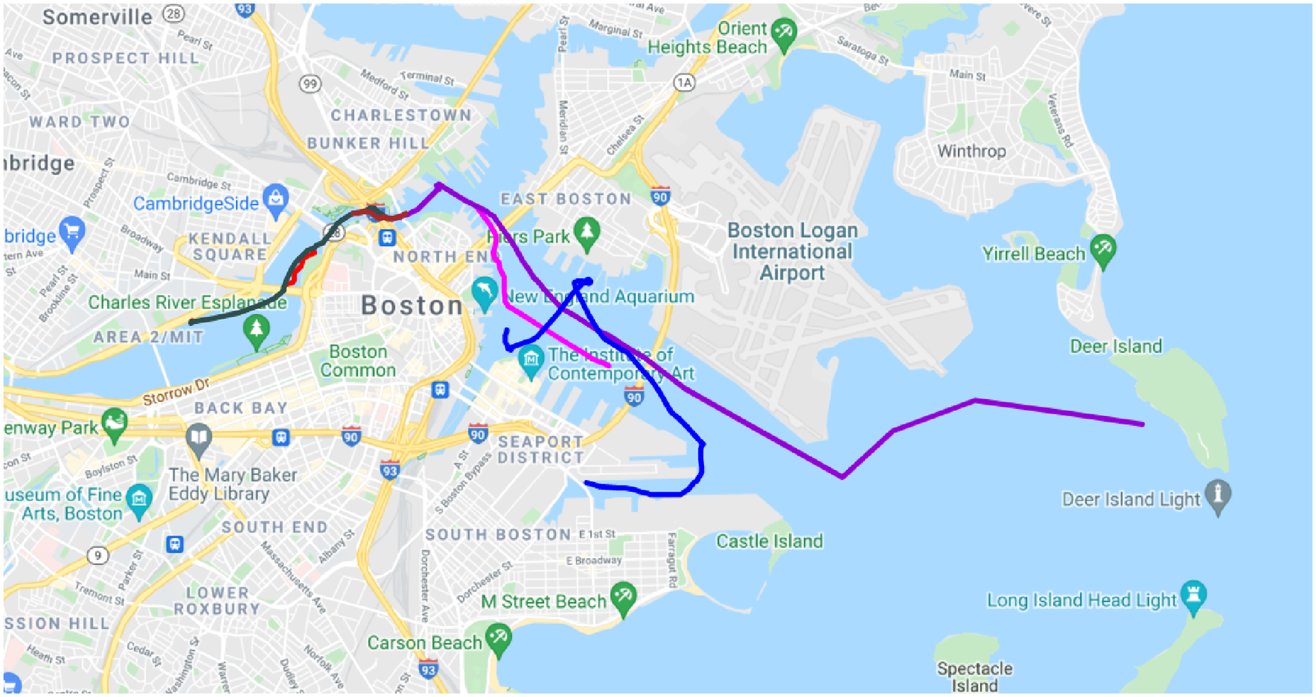

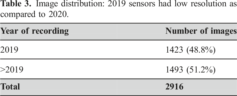
R/V Philos stores data from various sensors in the form of rosbag Staples (2020) files. LWIR and optical images were extracted from these rosbag files and carefully analyzed. One challenge faced while selecting LWIR images was the lack of texture and color information that sometimes undermined the scene complexity. In such cases, we used the corresponding optical equivalents to guide through the selection. The epoch time from the rosbag file was also used to specifically target scenes after sunset. This ensured that our dataset specifically included scenes that would pose challenges to the optical sensors. The resolution of 2019 footage was lesser than later recordings and helped create a variation that would be natural in a practical world. The dataset has approximately equal distribution of these images as indicated in Table 3.

Table 3.

Image distribution: 2019 sensors had low resolution as compared to 2020.

Year of recording	Number of images
2019	1423 (48.8%)
>2019	1493 (51.2%)
Total	2916

Intrinsically maritime scenes have a significant imbalance in their class distribution as compared to the ground scenes. Sky and water are present in almost any image and occupy major portions. While nearshore scenes help in capturing the real-life traffic and living presence, they also amplify the background adding to the disproportion. As part of the selection process, we tried to reduce this imbalance so that sky and background do not undermine the obstacles and living obstacles in the water that are critical for training. We also focused on bridges as a part of them was relevant for scene understanding while the remainder was not and therefore had to be considered as background. Another important difference between maritime and ground scenes is the line of sight. In maritime environment, cameras are exposed to large vistas and distant objects although part of the scene, can only be identified vaguely because they appear tiny. Annotation of such objects may vary as they become more discernible. Such reinterpretation requires consideration of distance as an additional parameter in the classifiers. Table 4 and Figure 5 show the size and instance distribution of each class in the dataset. The obstacles (purple) and living obstacles (green) mostly occupy less area but there are few instances in which they occupy considerably larger area. The images in such cases contain close up views of boat and/or humans. Figure 5 shows size variation across far obstacles, sky, and water in the order of magnitude.

Table 4.

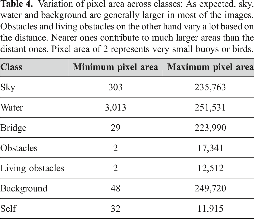
Variation of pixel area across classes: As expected, sky, water and background are generally larger in most of the images. Obstacles and living obstacles on the other hand vary a lot based on the distance. Nearer ones contribute to much larger areas than the distant ones. Pixel area of 2 represents very small buoys or birds.

Class	Minimum pixel area	Maximum pixel area
Sky	303	235,763
Water	3,013	251,531
Bridge	29	223,990
Obstacles	2	17,341
Living obstacles	2	12,512
Background	48	249,720
Self	32	11,915

Figure 5.

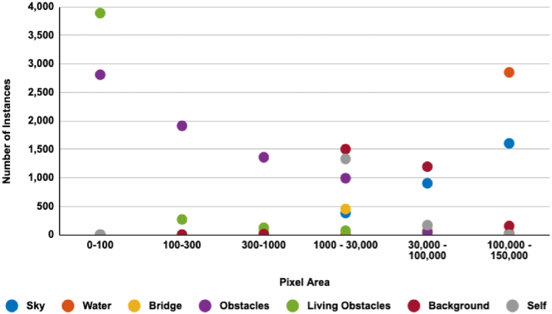
Distribution of instances across pixel area: As seen, sky, water, and background are prominently on the right end of the chart with larger area. Most of the concentration of living obstacles and obstacles is on the left indicating smaller pixel areas. There is a gradual progression toward the center which indicates cases where these obstacles are in close proximity and appear larger. Distance does play a role in bridge size as well but not to the same extent as that of obstacles. Training was therefore done on actual size images so that we can retain information for obstacles and living obstacles.

4.2. Image segmentation

The purpose of this and the next section is to share our experience of labeling the dataset with the research community. We believe that there are key lessons which the community can benefit from. We analyzed the Cityscape Cordts et al. (2016) dataset to understand the guidelines of their classification. In order to make our dataset meaningful for scene understanding, we finalized 7 classes—“sky,” “water,” “obstacle,” “living obstacle,” “bridge,” “background,” and “self” for annotation. Categorizing maritime scene into such refined classes ensures that true obstacles are identified and not get combined with other non-essential entities. The “obstacle” class consists of inanimate objects surrounded by water such as buoys, small platforms, sailboats, ships, and kayaks.

Animate obstacles like humans and birds in the water are classified as “living obstacles.” Though this class may seem contrived, identification of humans and marine wildlife may be useful for surveillance and environmental or ecological monitoring, respectively. Illegal trafficking of drugs, weapons, and humans through marine channels is a vexing problem and such activities are often carried out at night. Detecting humans in such cases may prove to be useful. In the future world of USVs, probably being able to detect a human on board might also prove useful. Thus, the dataset can be used for multiple purposes.

Because of the urban setting of the dataset, bridges were frequent and posed a unique challenge. The piers of the bridge that are submerged in water and the girder of the bridge were relevant as the ASV would need to maneuver around the same. However, the top of the bridge was not hence we annotated the navigation relevant portions of the bridge as “bridge” class and mark the remaining portions as “background” class. The “background” class covered any static or dynamic entities that were on land such as trees, buildings, and construction cranes.

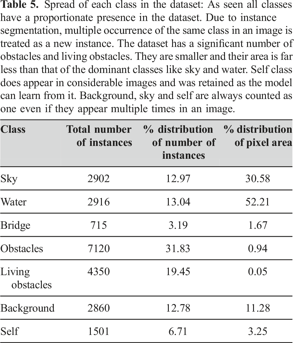
We observed self returns on the images due to the position of the cameras and these have been labeled as “self” class. This area neither represents “obstacle” nor “background” and hence justified its own label. Table 5 shows number of instances in each class that were annotated in these images and also the distribution of pixel area across these classes.

Table 5.

Spread of each class in the dataset: As seen all classes have a proportionate presence in the dataset. Due to instance segmentation, multiple occurrence of the same class in an image is treated as a new instance. The dataset has a significant number of obstacles and living obstacles. They are smaller and their area is far less than that of the dominant classes like sky and water. Self class does appear in considerable images and was retained as the model can learn from it. Background, sky and self are always counted as one even if they appear multiple times in an image.

Class	Total number of instances	% distribution of number of instances	% distribution of pixel area
Sky	2902	12.97	30.58
Water	2916	13.04	52.21
Bridge	715	3.19	1.67
Obstacles	7120	31.83	0.94
Living obstacles	4350	19.45	0.05
Background	2860	12.78	11.28
Self	1501	6.71	3.25

As we were working through the annotations, many images gave us new insights that had to be incorporated. We had anticipated bridge complexity as part of our planning; however, we encountered a similar issue with respect to obstacles. Initially, we defined an obstacle as an entity surrounded by water on all sides. However, we came across construction objects that stretched from land into the water such as gates that allow the boats to pass through, piers and docks to park the boats, or platforms connected to the land. These obstacles were pertinent for scene classification and hence could not be treated as background. Similarly birds flying just above the water were categorized as sky, and birds in the water were categorized as “living obstacle.” Since the images are 2D and LWIR does not give a good feel of the color and texture, there were cases where the obstacle in water was collapsed in the rear background and had to be reviewed thoroughly. Another challenge faced was due to the wide and deep line of sight that we get in the marine environment. There were many obstacles near the horizon that were very tiny. We had to enlarge the image and annotate such images per pixel. A person on a boat is annotated as a “living obstacle” while the boat is annotated as an “obstacle.” In cases where the boat was far out and a human could not be easily identified on the boat, it was not called out and considered as part of the “obstacle” class.

In addition to labeling, we also had to make a choice between semantic and instance segmentation. In semantic segmentation, each occurrence of a class is assigned same class label while in instance segmentation, each instance of a class is assigned different instance ID. Unlike on land, maritime environment has a wide and deep line of sight. The near and far objects may overlap in the 2D view of an image. They will be collapsed if semantic segmentation was used. By instance segmenting the image, the information of overlapping multiple obstacles can be retained which in turn can be used to evaluate or develop occlusion aware classifier vital for path planning. Lastly, the benefit of instance segmentation is that it can always be converted programmatically to semantic based on the need. Figure 6 illustrates a few samples of raw LWIR images and their annotated masks.

Figure 6.

LWIR images and their segmentation: Multiple occurrences of birds, humans or boats have their own instance id and appear in different color. Background, sky, and water each have only one instance in an image.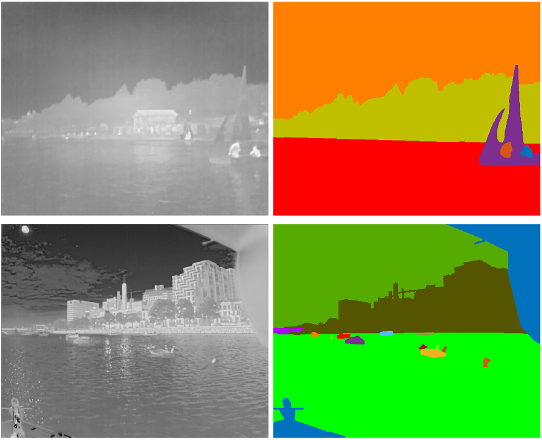

4.3. Labeling process

An independent organization was tasked with the labeling of these images. To achieve consistency in the result, we created and shared a detailed class label definition document so that labelers would have a common understanding. We also labeled a batch of images ourselves to illustrate the desired outcome. There are many tools available for image segmentation but we chose segments.ai Debals (2021) platform because of its ease of use. The labeling was quick because of its superpixel technology. The API interface made working with the labeled dataset efficient. Figure 7 shows the tool in action. While the labeling tool was easy to use, there were some challenges faced especially due to the nature of LWIR images. Lack of color and textures posed difficulties in image identification as well as annotation. Color and texture assists the human eye in making a judgment. Lack of thereof, led to multiple reviews in some complex situations such as cluttered set of obstacles, cluster of parking poles, flock of birds, or distant ships. For each LWIR video, the corresponding optical version was therefore provided to the labeling team for reference. The image had to be classified in 7 classes. This made the labeling process quite elaborate and time consuming. Identifying parts of the bridge that should be annotated as background was subjective and as a result, there may be some deviations in some of the annotations. In summary, the semantic annotation exercise for LWIR images was more time consuming and needed a lot more attention than we had anticipated. On the positive side, the tool had a zoom-in capability and allowed us to annotate tiny areas of the order of few pixels well. We wanted to account for all sizes of the obstacles because we wanted our dataset to be a real-life dataset. Instead of all perfect images, presence of extremities can make the dataset more robust.

Figure 7.

Image segmentation platform: Segments.ai tool that was used for annotation. It provides super pixels that improve the productivity and reduces manual errors. Pipeline was automated using the API interface.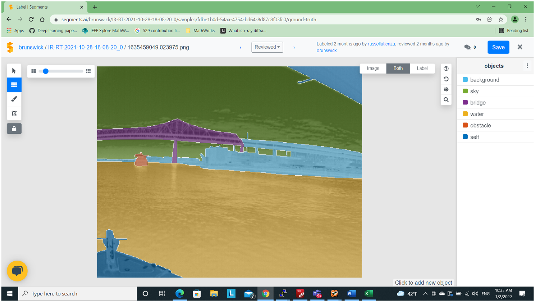

Two rounds of reviews were done to improve the accuracy of segmentation. Including the reviews, each image annotation took approximately 25 min. We also developed a script to check for any unclassified pixels and corrected such masks. Automated checks for validating the segmentation and gathering metrics were also developed.

5. Dataset evaluation

Though we have created instance-segmentation dataset, for the purpose of evaluation we used its semantic segmentation masks. To evaluate the efficacy of the dataset, we used 3 image segmentation architectures - UNet developed earlier by Ronneberger et al. (2015) for medical image segmentation, PSPNet by Zhao et al. (2017) for its improvement over fully convolutional network based segmentation and DeepLabv3 by Chen et al. (2018) which is known for its overall superior performance. The dataset was split into 3 categories - 70% for training, 20% for validation and 10% for testing. The test images were used only during inference. Pretrained weights such as Deng et al. (2009) are generally available for training optical images. They greatly reduce the time to retrain the model; however, these do not work well for LWIR image training as shown by Nirgudkar and Robinette (2021). Another challenge was the characteristics of these images. The pixel area occupied by the boats (0.94%) is the second least because they are tiny as compared to the water or sky in an image. We therefore trained these architectures from scratch for our LWIR dataset to mitigate such issues. Image resolution of 640 × 512 (width×height) pixels was used across all the architectures - UNet (Ronneberger et al. (2015)), PSPNet (Zhao et al. (2017)), DeepLabv3 (Chen et al. (2018)) for both 2019 as well as the 2020 images. Note that even though 2019 cameras had a resolution of 320 × 256, the saved images had a size of 640 × 512.

5.1. Data augmentation

Robust, diverse and large volume of data is a prerequisite for any successful model. However, creating a labeled dataset is a laborious and expensive task. A common technique employed in increasing the dataset variety is data augmentation Schöller et al. (2019), Bovcon et al. (2019). We used the following two types of transformations for our dataset:

• Rotation: An image and its mask were rotated by ±2°, ±5°, ±7°

• Mirror: The original image and mask and their rotated equivalence from previous step was mirrored on the vertical axis

This scheme generated 13 images from one image. Accordingly, our dataset was augmented to 40,096 images. An illustrative example is shown in Figure 8.

Figure 8.

Data augmentation: First column shows original image and its mask followed by 3 rotations: 2, 5 and 7° respectively. Last column shows mirror operation. Images were also rotated by −2, −5, and −7°.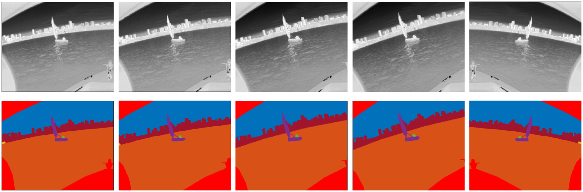

5.2. Performance criterion

Intersection over union (IoU) is an important metric for segmentation inference Csurka et al. (2013). It is defined as ratio of area of intersection between predicted segmentation mask (P) and the ground truth (G), and the area of union between the two.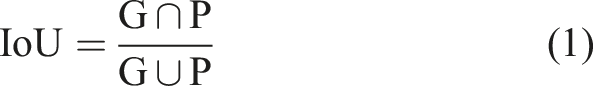

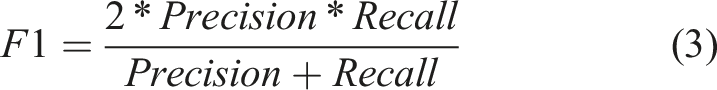
IoU = \frac{G \cap P}{G \cup P}

(1)

The IoU score ranges between 0 and 1. A threshold value can be chosen to determine if the inference can be treated as true positive (TP). If the IoU score is greater than a certain threshold, then we treat the inference as true positive (TP) otherwise it is treated as false negative (FN). If the ground truth does not contain the region present in prediction then it is treated as false positive (FP). Usually, a threshold value of greater than 0.5 is considered optimal Liu et al. (2021); however, if the class sizes are tiny as in the present case, the threshold can be compromised to a lower value. The precision, recall and F1 score are defined as follows:

P r e c i s i o n (\Pr) = \frac{T P}{T P + F P}, R e c a l l (Re) = \frac{T P}{T P + F N}

(2)

F 1 = \frac{2 * P r e c i s i o n * R e c a l l}{P r e c i s i o n + R e c a l l}

(3)

5.3. Performance metrics

All 3 architectures were run on Google Colab platform which provided a 16 GB GPU memory. Training was performed from scratch without using pretrained weights. Images were randomly shuffled prior to the training which helped in improving the robustness of the model. Table 6 gives a summary of the high level metrics obtained for each architecture.

Table 6.

Performance of various architectures: Size of the images and number of epochs were identical across the 3 architectures.

Name	Images	Image size	Epoch	Loss	Training time
UNet	train:27678			0.0202	27 h 50 min
PSPNet	val:7910	640*512	50	0.0223	47 h 56 min
DeepLabv3	test:4508	640*512	50	0.0112	29 h 30 min

The two most commonly occurring classes are water and sky. In some images, clouds are present in the sky but there is no such “pollution” for water. When obstacles, bridges or background is present, these regions are classified as such leaving water areas almost perfect. This is the reason why inference for water is 100%. The training loss (sparse categorical cross entropy) is quite low for all the three architectures. However, since water and sky occupy significant portions of the maritime images, this parameter does not help much and gives misleading accuracy. Classes were therefore individually analyzed and Table 7 reports these metrics at a class level. As noted above, sky and water have a significant contribution in each image and therefore yield a high F1 even with a threshold of 0.6. The classes that are critical for scene understanding namely “obstacles,” “living obstacles,” and “bridge” are much smaller as per Figure 5. As shown in Table 7, a threshold of 0.6 gives substantial FNs for “obstacles” and “living obstacles.” Since the pixel area of these classes is really tiny, we decided to evaluate their performance by lowering the threshold to 0.3. As seen from the table, the FN reduced appreciably. The threshold value can be subjective based on the size of the class. A value of 0.6 for tiny sizes is too high a bar to achieve. The primary intent of the model is scene understanding and having a dynamic threshold based on parameters like size or distance would enable the model to predict the presence of an obstacle although it may have lesser spatial accuracy. Poor recall score of PSPNet on “living obstacles” indicates its failure to identify them which is also reflected in low F1 score.

Table 7.

Quantitative results on the MassMIND dataset: Classes pertinent to the scene understanding were also evaluated against a lower threshold. PSPNet performs at par with DeepLabv3 in all classes except for ‘living obstacles’ as indicated by the poor recall. Most of the times it identifies the living obstacle but collapses it in the obstacle (a boat typically). Large number of epochs for PSPNet will probably circumvent this problem. However, its F1 score for obstacles is marginally better than DeepLabv3. Despite their tiny size, obstacles give a satisfactory recall. F1 score of DeepLabv3 for bridge, obstacle, and living obstacle classes is quite good. It has performed well across all the classes.

Model	Class	Th	TP	FP	FN	Pr	Re	F1
UNet	Sky	0.6	4327	24	153	99.4	96.6	98.0
DeepLabv3			4374	8	106	99.8	97.6	98.7
PSPNet			4408	18	72	99.6	98.4	99.0
UNet	Water	0.6	4508	0	0	100	100	100
DeepLabv3			4508	0	0	100	100	100
PSPNet			4508	0	0	100	100	100
UNet	Bridge	0.6	723	605	409	54.4	63.9	58.8
UNet		0.3	962	605	170	61.4	85.0	71.3
DeepLabv3		0.6	870	377	262	69.8	76.9	73.1
DeepLabv3		0.3	1013	377	119	72.9	89.5	80.3
PSPNet		0.6	910	319	222	74.0	80.4	77.1
PSPNet		0.3	1040	319	92	76.5	91.9	83.5
UNet	Obstacle	0.6	615	504	2193	55.0	21.9	31.3
UNet		0.3	1645	504	1163	76.5	58.6	66.4
DeepLabv3		0.6	1143	429	1665	72.7	40.7	52.2
DeepLabv3		0.3	2045	429	763	82.7	72.8	77.4
PSPNet		0.6	1175	428	1633	73.3	41.8	53.3
PSPNet		0.3	2068	428	740	82.9	73.6	78.0
UNet	Living ob	0.6	98	136	886	41.9	10.0	16.1
UNet		0.3	420	136	564	75.5	42.7	54.5
DeepLabv3		0.6	294	141	690	67.6	29.9	41.4
DeepLabv3		0.3	599	141	385	80.9	60.9	69.5
PSPNet		0.6	65	9	1045	87.8	5.9	11.0
PSPNet		0.3	127	9	983	93.4	11.4	20.4
UNet	Background	0.6	3856	85	526	97.8	88.0	92.7
DeepLabv3			4049	33	333	99.2	92.4	95.7
PSPNet			4178	50	204	98.8	95.3	97.0
UNet	Self	0.6	2306	179	74	92.8	96.9	94.8
DeepLabv3			2322	54	58	97.7	97.6	97.6
PSPNet			2329	19	51	99.2	97.9	98.5

Figure 9 indicates the inference results from all 3 architectures for a few sample images. Living obstacles (humans) have been inferred really well in both DeepLabv3 and UNet. The boundaries separating humans from the obstacle (boat) has been interpreted well. In the second row, very tiny obstacles (birds) in the water have been correctly inferred by DeepLabv3 and UNet. Third row indicates that curvature or waves in water pose no issue to the model. Reflection in water in the fourth row, or the heavy cloud cover right on top of the sea, has been interpreted properly by the models. PSPNet was found to have problems with identifying “living obstacles.” While it works really well for all other classes, it needs a lot of training to consistently differentiate the boundaries between obstacle and the living obstacle.

Figure 9.

Qualitative comparison of the inference: First row: DeepLabv3 and UNet have a good inference other than a few traces of sky in the obstacle. PSPNet, despite the significant size has problem in identifying living obstacles and will need significant additional training. Second row: Very tiny birds in the water have been correctly captured by both DeepLabv3 and UNet and are again missed in PSPNet. Third row: Curvature of the image and waves in water have been correctly depicted in all 3 classifiers. DeepLabv3 does a good job in calling out the bridges as well. Fourth row: There is significant reflection in the water that is handled well by all, except for a few sporadic traces of bridge. Fifth row: There is a very obscure cloud and sky boundary. The image was taken in relatively open waters, see one of the routes in Fig. 4. This has been handled really well in all 3 models. Overall, glitter, waves, horizon boundaries that are a problem in optical world are handled well in the LWIR dataset. DeepLabv3 performs best overall, closely followed by PSPNet (except for the problem with living obstacle) and UNet.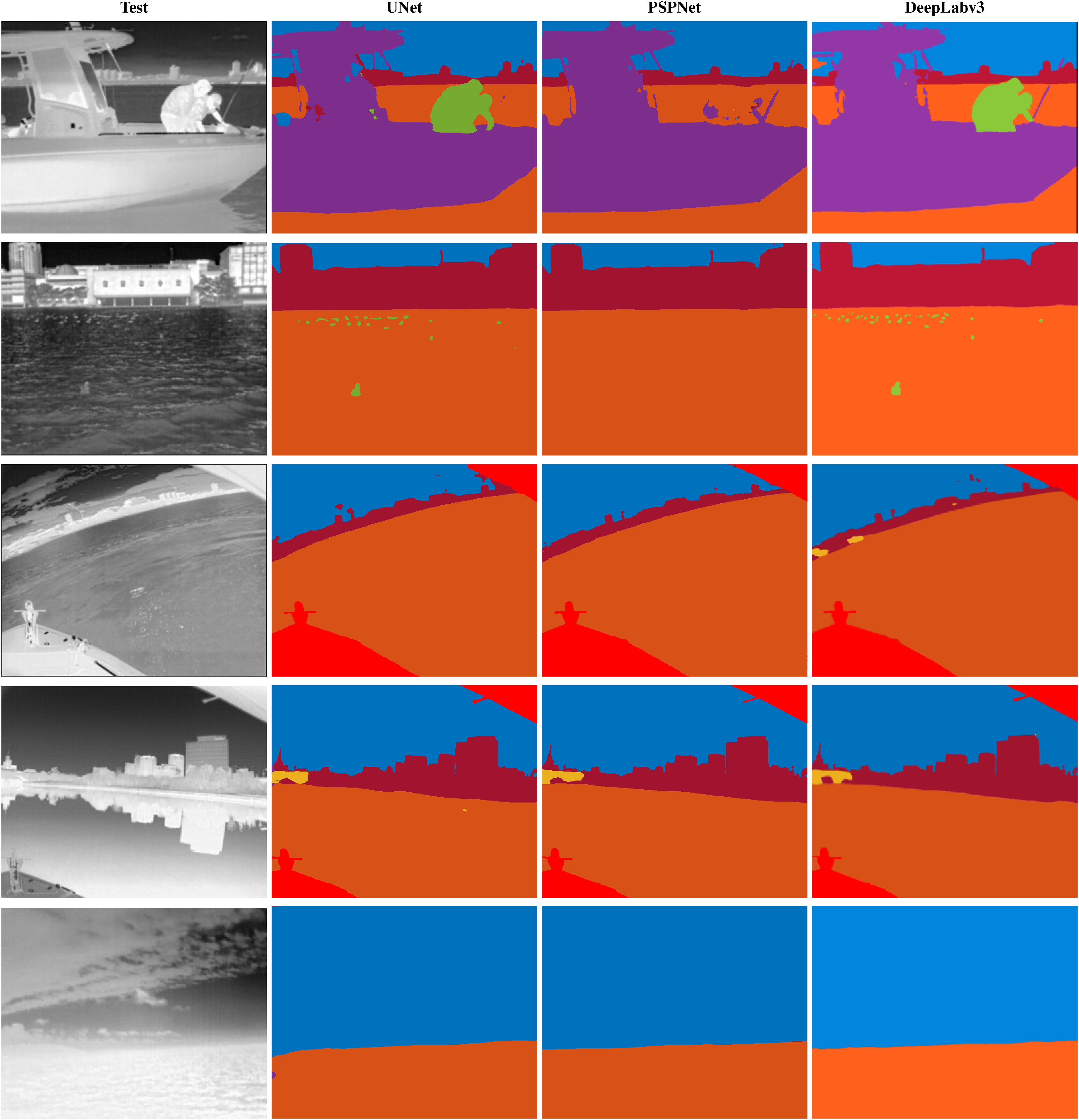

In addition to the above limitation in PSPNet, there were some situations where very tiny obstacles were missed or not completely identified. Bridge is another area where the classifiers sometimes gave inconsistent results. This was primarily due to the fact that ground truth for the bridge contained a portion annotated as ‘background’ that is not pertinent to navigation. The classifier therefore sometimes incorrectly inferred the navigable portion of the bridge as background and vice versa. Despite that, inference for “bridge” class improved significantly after increasing the training to 50 epochs. Some of the challenge cases are shown in Figure 10.

Figure 10.

Misrepresented inference: First row: A portion of the obstacle has been clubbed with the background in both UNet and DeepLabv3, however it is represented properly in PSPNet. There are sporadic traces of bridge in UNet. Second row: Again, the hull of the larger ship is very close to the background and the classifier has problems detecting the boundaries in all 3 architectures. And there are a few spurious occurrences of bridge and living obstacles. Third row: PSPNet has a better inference than the rest although the boundaries are not clear. Portions of bridge and background have been collapsed in the other two along with a few sporadic obstacles. The reflection in water has been handled well in all three.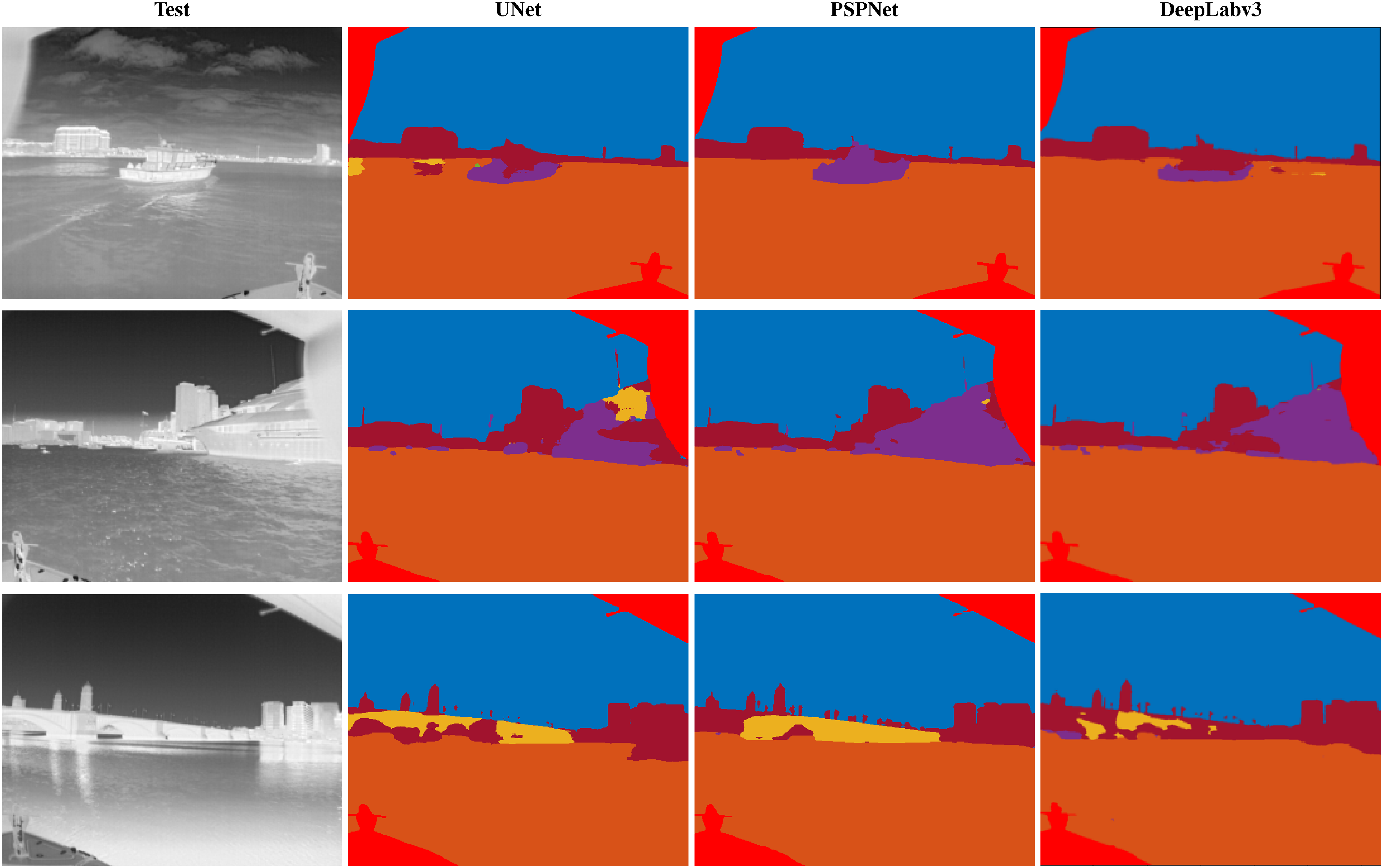

To get consistent and meaningful performance from the deep learning models, various modifications were tried and parameters changed. A few of those key modifications are elaborated below:

Initially we had reduced the image size to 320 × 256 (width×height) to speed up the training phase. This resulted in a lot of smaller obstacles being missed in the inference. The obstacles were inherently small as shown in Table 4 and they got tinier with the reduction in image size leaving the classifier with very little information to train well. It was therefore decided to retain the original size of the images. We also experimented with excluding 2019 images because they were of low resolution. We expected improvement in the performance. However, the performance worsened as a lot of variation and information contained in the 2019 dataset was lost. We therefore retained both 2019 and 2020 images.

To increase the dataset size, data augmentation was used as described in Sub-Section 5.1. For optical images, color adjustment is yet another augmentation operation. However, augmentation by changing the brightness of LWIR images had adverse effect on the inference and was not incorporated. Larger rotations (±10°, ±15°) were tried and that caused distortion in 2019 images and deteriorated the overall results. Smaller range ( ±2°, ±5°, ±7°) seem to fit the dataset well. An important consideration that improved the performance drastically was shuffling. Since our images were named based on epoch times, without explicit shuffling they were fed sequentially to the classifier and gave poor results. They were shuffled randomly before the training and that variation helped the classifiers boost the performance multi-fold.

As seen from the inference, horizon detection does not pose a problem in LWIR images. However, there are some sporadic instances of clouds being incorrectly inferred as water and vice versa. This happens mainly when there are white clouds in the sky that appear similar to water, have similar pixel values and get labeled incorrectly. Bridge annotation remained challenging despite good F1 scores. Depending on the nature of the bridge and position of the background with respect to the bridge, the classifier has a challenge and classifies the navigable portion of the bridge as a background. When the bridge has arches, view from beneath the arch could be sky or background and water. Such minute details pleasantly have been represented well most of the times, but do pose a challenge in other cases.

In summary, standard CNN architectures can be trained with LWIR images and can produce good inference for obstacle detection and scene understanding. Although EO cameras are better suited for boat classification, in extreme light conditions they perform poorly in their ability to detect an obstacle. In such cases, LWIR cameras can assist in detection if not in the categorization. It may not be COLREG compliant but it would at least detect the obstacles and indicate the relative positions of obstacles, water, background etc. Thus, the LWIR dataset complements the optical dataset in scenarios where lighting conditions are extreme and is therefore invaluable in the perception task.

6. Conclusion

We have presented a comprehensive MassMIND dataset containing over 2900 segmented diverse LWIR images and made it publicly available. This is the first maritime dataset that segments LWIR images in 7 different classes with emphasis on living and non-living, static and dynamic obstacles in the water. It can be used for a variety of use cases. Additionally, any label can be collapsed in another label programmatically if it is not of interest. The dataset is evaluated and bench marked against a few industry standard architectures.

Of the 3 classifiers evaluated, DeepLabv3 Chen et al. (2018) stands out the best, followed by UNet and PSPNet. PSPNet is found to be comparable to DeepLabv3 in all other classes except for living obstacles. Our research calls out significance of LWIR when it comes to problems such as extreme light conditions and horizon detection that are common in the optical world. In addition, the dataset tries to encompass many of the critical aspects of the maritime imagery such as static and dynamic obstacles of varying sizes, crowded shoreline, deep seas, varying weather and light patterns, and life presence on the water surface. Such a diverse LWIR dataset can be useful to improve the deep learning architectures for the maritime environment. At the same time, it can complement optical datasets. The present dataset also has some limitations. Certain obstacles such as river barges or Sea-Doos are not captured because of the ASVs’ urban setting. The demographics within the dataset is also limited to one region in USA. We understand that as a result, there is no variety in navigational markers used across world regions. This gap can be bridged by collaboration with other researchers.

LWIR images lack texture and color information so classifying boats into subclasses will take more effort. However, we plan to refine the current ‘obstacle’ class to indicate the type of obstacle such as sailboats, kayaks, and merchant ships. For tug boats, cargos, and tankers additional parameter of a safe zone criterion can be incorporated. We are also exploring labeling of the data from other sensors such as radar or lidar that will be synchronized with LWIR and EO cameras. This will enable creation of dataset and classifiers which can be useful for navigation. We demonstrated a prototype of integration of inference obtained by LWIR sensor, radar, and lidar in Nirgudkar and Robinette (2022). We plan to further refine that research such that it can work in real time. Lastly, we will also explore creation of an instance-segmentation architecture dedicated towards LWIR images in the marine environment.

Footnotes

Acknowledgements

We are grateful to Brunswick^® Corporation for their support. The views, opinions and/or findings expressed are those of the authors and should not be interpreted as representing the official views of Brunswick^® Corporation. We also thank the team at segments.ai for providing early access free of charge and for providing dashboard for tracking the progress of the labeling work.

Declaration of conflicting interests

The author(s) declared no potential conflicts of interest with respect to the research, authorship, and/or publication of this article.

Funding

The author(s) received no financial support for the research, authorship, and/or publication of this article.

ORCID iDs

Shailesh Nirgudkar

Michael DeFilippo

References

AUVLab (1989) MIT Sea Grant. Autonomous Underwater Vehicles Lab URL https://seagrant.mit.edu/auv-lab/

Bloisi

Iocchi

Pennisi

, et al. (2015) ARGOS-venice boat classification. 12th IEEE International Conference on Advanced Video and Signal Based Surveillance (AVSS): 1–6. DOI: 10.1109/AVSS.2015.7301727.

Bovcon

Kristan

(2020) A water-obstacle separation and refinement network for unmanned surface vehicles. IEEE International Conference on Robotics and Automation, ICRA 2020. 2020: 9470–9476. DOI: 10.1109/ICRA40945.2020.9197194.

Bovcon

Muhovič

Perš

, et al. (2019) The MaSTr1325 Dataset for Training Deep Usv Obstacle Detection Models. IEEE/RSJ International Conference on Intelligent Robots and Systems (IROS).

Bovcon

Muhovič

Vranac

, et al. (2021) MODS- A USV-Oriented Object Detection and Obstacle Segmentation Benchmark.

Castellini

Bloisi

Blum

, et al. (2020) Intcatch Aquatic Drone Sensor Dataset. Mendeley Data. V2 . DOI: 10.17632/gtt7stf5x8.2.

Chen

Papandreou

Kokkinos

, et al. (2018) Deeplab: Semantic image segmentation with deep convolutional nets, atrous convolution, and fully connected CRFs. IEEE TPAMI 40(4): 834–848.

Cordts

Omran

Ramos

, et al. (2016) The Cityscapes Dataset for Semantic Urban Scene Understanding. Proc. Of the IEEE Conference on Computer Vision and Pattern Recognition (CVPR).

Csurka

Larlus

Perronnin

, et al. (2013) What is a good evaluation measure for semantic segmentation? Bmvc 27: 10–5244.

10.

Debals

(2021) Platform for Image Segmentation URL https://segments.ai.

11.

DeFilippo

Sacarny

Robinette

(2021) RoboWhaler: A Robotic Vessel for Marine Autonomy and Dataset Collection. OCEANS.

12.

Deng

Dong

Socher

, et al. (2009) Imagenet: A large scale hierarchical database. CVPR: 248–255.

13.

Edmund Optics (2022). What is SWIR? URL https://www.edmundoptics.com/knowledge-center/application-notes/imaging/what-is-swir/?utm_medium=email&utm_source=transaction

14.

Hyll

(2016) Image-based Quantitative Infrared Analysis and Microparticle Characterisation for Pulp and Paper Applications. DOI: 10.13140/RG.2.1.2595.6884.

15.

Krizhevsky

Sutskever

Hinton

(2012) Imagenet classification with deep convolutional neural networks. Advances in Neural Information Processing Systems 25: 1097–1105.

16.

Liu

Geng

Zhao

, et al. (2021) Image semantic segmentation use multiple-threshold probabilistic R-CNN with feature fusion. Symmetry 13: 207.

17.

NASA (2003) Near. Mid and Far Infrared URL http://www.icc.dur.ac.uk/tt/Lectures/Galaxies/Images/Infrared/Regions/irregions.html

18.

Nirgudkar

DeFilippo

Sacarny

, et al. (2022) MassMIND: Massachusetts Maritime INfrared Dataset URL https://github.com/uml-marine-robotics/MassMIND

19.

Nirgudkar

Robinette

(2021) Beyond visible light: Object Detection Using Long Wave Infrared Images in Maritime Environment. International Conference on Autonomous Robotics.

20.

Nirgudkar

Robinette

(2022) Obstacle tracking in marine environment with long wave infrared in multisensor fusion. Robotic Perception and Mapping: Emerging Techniques, ICRA Workshop.

21.

Patino

Cane

Vallee

, et al. (2016) PETS 2016: Dataset and Challenge. IEEE Conference on Computer Vision and Pattern Recognition Workshops (CVPRW): 1240–1247. DOI: 10.1109/CVPRW.2016.157.

22.

Prasad

Rajan

Rachmawati

, et al. (2017) Video processing from electro-optical sensors for object detection and tracking in maritime environment: a survey. IEEE Transactions on Intelligent Transportation Systems 18(8): 1993–2016.

23.

Dai

, et al. (2011) Fast detection of small infrared objects in maritime scenes using local minimum patterns. 18th IEEE International Conference on Image Processing: 3553–3556. DOI: 10.1109/ICIP.2011.6116483.

24.

Ribeiro

Cruz

Matos

, et al. (2019) A data set for airborne maritime surveillance environments. IEEE Transactions on Circuits and Systems for Video Technology 29(9): 2720–2732.

25.

Robinette

Sacarny

DeFilippo

, et al. (2019) Sensor Evaluation for Autonomous Surface Vehicles in Inland Waterways. OCEANS.

26.

Rodin

Johansen

(2018) Detectability of objects at the sea surface in visible light and thermal camera images. OCEANS - MTS/IEEE Kobe Techno-Oceans (OTO). DOI: 10.1109/OCEANSKOBE.2018.8559310.

27.

Ronneberger

Fischer

Brox

(2015) U-Net: convolutional networks for biomedical image segmentation. Medical Image Computing and Computer-Assisted Intervention (MICCAI) 9351: 234–241. DOI: 10.1007/978-3-319-24574-4_28.

28.

Schöller

FET

Plenge-Feidenhans’l

Stets

, et al. (2019) Assessing deep-learning methods for object detection at sea from LWIR images. International Federation of Automatic Control Workshop 52(21): 64–71. DOI: 10.1109/OCEANSKOBE.2018.8559310.

29.

SeaGrant (2022) MIT Sea Grant Marine Perception Dataset URL https://seagrant.mit.edu/auvlab-datasets-marine-perception-1

30.

Staples G (2020) Rosbag package URL http://wiki.ros.org/rosbag

31.

Steccanella

Bloisi

Castellini

, et al. (2020) Waterline and obstacle detection in images from low-cost autonomous boats for environmental monitoring. Robotics and Autonomous Systems 124: 103346. DOI: 10.1016/j.robot.2019.103346.

32.

Wang

Dong

Zhao

, et al. (2017) Fast infrared maritime target detection: Binarization via histogram curve transformation. Infrared Physics and Technology 83: 32–44. DOI: 10.1016/j.infrared.2017.03.009.

33.

Zhang

Choi

Daniilidis

, et al. (2015) VAIS: A dataset for recognizing maritime imagery in the visible and infrared spectrums. IEEE Conference on Computer Vision and Pattern Recognition Workshops (CVPRW): 10–16. DOI: 10.1109/CVPRW.2015.7301291.

34.

Zhao

Shi

, et al. (2017) Pyramid scene parsing network. IEEE Conference on Computer Vision and Pattern Recognition (CVPR) : 6230–6239. DOI: 10.1109/CVPR.2017.660.