Combining learned and analytical models for predicting action effects from sensory data

Abstract

One of the most basic skills a robot should possess is predicting the effect of physical interactions with objects in the environment. This enables optimal action selection to reach a certain goal state. Traditionally, dynamics are approximated by physics-based analytical models. These models rely on specific state representations that may be hard to obtain from raw sensory data, especially if no knowledge of the object shape is assumed. More recently, we have seen learning approaches that can predict the effect of complex physical interactions directly from sensory input. It is, however, an open question how far these models generalize beyond their training data. In this work, we investigate the advantages and limitations of neural-network-based learning approaches for predicting the effects of actions based on sensory input and show how analytical and learned models can be combined to leverage the best of both worlds. As physical interaction task, we use planar pushing, for which there exists a well-known analytical model and a large real-world dataset. We propose the use of a convolutional neural network to convert raw depth images or organized point clouds into a suitable representation for the analytical model and compare this approach with using neural networks for both, perception and prediction. A systematic evaluation of the proposed approach on a very large real-world dataset shows two main advantages of the hybrid architecture. Compared with a pure neural network, it significantly (i) reduces required training data and (ii) improves generalization to novel physical interaction.

1 Introduction

We approach the problem of predicting the consequences of physical interaction with objects in the environment based on raw sensory data. Traditionally, interaction dynamics are described by a physics-based analytical model (Lynch et al., 1992; Yu et al., 2016; Zhang and Trinkle, 2012), which relies on a certain representation of the environment state. This approach has the advantage that the underlying function and the input parameters to the model have physical meaning and can therefore be transferred to problems with variations of these parameters. They also make the underlying assumptions in the model transparent. However, defining such models for complex scenarios and extracting the required state representation from raw sensory data may be very difficult, especially if no assumptions about the shape of objects are made.

More recently, we have seen approaches that successfully replace the physics-based models with learned ones (Bauza and Rodriguez, 2017; Belter et al., 2014; Kopicki et al., 2017; Mericli et al., 2015; Zhou et al., 2016). While often more accurate than analytical models, these methods still assume a predefined state representation as input and do not address the problem of how it may be extracted from raw sensory data.

Some neural-network-based methods instead simultaneously learn a representation of the input and the associated dynamics from large amounts of training data (e.g., Agrawal et al., 2016; Byravan and Fox, 2017; Finn et al., 2016;Watters et al., 2017). They have shown impressive results in predicting the effect of physical interactions. Agrawal et al. (2016) argued that a neural network may benefit from choosing its own representation of the input data instead of being forced to use a predefined state representation. They reasoned that a problem can often be parametrized in different ways and that some of these parametrizations might be easier to obtain from the given sensory input than others. The disadvantage of a learned representation is, however, that it usually cannot be mapped to physical quantities. This makes it difficult to intuitively understand the learned functions and representations. In addition, it remains unclear how these models could be transferred to similar problems. Neural networks often have the capacity to memorize their training data (Zhang et al., 2016) and learn a mapping from inputs to outputs instead of the “true” underlying function. This can make perfect sense if the training data covers the whole problem domain. However, when data is sparse (e.g., because a robot learns by experimenting), the question of how to generalize beyond the training data becomes very important.

Our hypothesis is that using prior knowledge from existing physics-based models can provide a way to reduce the amount of required training data and at the same time ensure good generalization beyond the training domain. In this article, we thus investigate using neural networks for extracting a suitable representation from raw sensory data that can then be consumed by an analytical model for prediction. We compare this hybrid approach with using a neural network for both, perception and prediction, and with the analytical model applied on ground-truth input values.

As example physical interaction task, we choose planar pushing. For this task, a well-known physical model (Lynch et al., 1992) is available as well as a large, real-world dataset (Yu et al., 2016) that we augmented with simulated images. Given a depth image of a tabletop scene with one object and the position and movement of the pusher, our models need to predict the object position in the given image and its movement due to the push. Although the state-space of the object is rather low-dimensional (2D position plus orientation), pushing is already a quite complex manipulation problem: the system is under-actuated and the relationship between the push and the object movement is highly nonlinear. The pusher can slide along the object and dynamics change drastically when it transitions between sticking and sliding contact or makes and breaks contact.

Our experiments show that despite of relying on depth images to extract position and contact information, all our models perform similar to the analytical model applied on the ground-truth state. Given enough training data and evaluated inside of its training domain, the pure neural network implementation performs best and even outperforms the analytical model baseline significantly. However, when it comes to generalization to new actions the hybrid approach is much more accurate. In addition, we find that the hybrid approach needs significantly less training data than the neural network model to arrive at a high prediction accuracy.

1.1 Contributions

In this work, we make the following contributions.

• We show how analytical dynamics models and neural networks can be combined and trained end-to-end to predict the effects of robot actions based on depth images or organized point clouds.

• We compare this hybrid approach with using a pure neural network for learning both, perception and prediction. Evaluations on a real-world physical interaction task demonstrate improved data efficiency and generalization when including the analytical model into the network over learning everything from scratch.

• We show how the hybrid approach can be further extended by combining the analytical model with a learned error-correction term to better compensate for possible inaccuracies of the analytical model

• For training and evaluation, we augmented an existing dataset of planar pushing with depth and RGB images and additional contact information. The code for this is available online.

1.2 Outline

This article is structured as follows. We begin with a review of related work in Section 2. In Section 3, we formally describe the problem we address, introduce an analytical model for planar pushing (Section 3.1), and the dataset we used for our experiments (Section 3.2).

Section 4 introduces and compares the different approaches for learning perception and prediction. The evaluation in Section 5 compares data-efficiency (Section 5.3) and generalization abilities (Sections 5.4, 5.5, and 5.6) of the different architectures. The perception task is kept simple for these experiments by using a top-down view of the scene. This changes in Section 6 where we demonstrate that the hybrid approach also performs well in a less-constrained visual setup. Section 7 finally summarizes our results and gives an outlook to future work.

2 Related work

2.1 Models for pushing

Analytical models of quasi-static planar pushing have been studied extensively in the past, starting with Mason (1986). Goyal et al. (1991) introduced the limit surface to relate frictional forces with object motion, and much work has been done on different approximate representations of it (Hong Lee and Cutkosky, 1991; Howe and Cutkosky, 1996). In this work, we use a model by Lynch et al. (1992), which relies on an ellipsoidal approximation of the limit surface.

More recently, there has also been a lot of work on data-driven approaches to pushing (Bauza and Rodriguez, 2017; Belter et al., 2014; Kopicki et al., 2017; Meriçli et al., 2015; Zhou et al., 2016). Kopicki et al. (2017) described a modular learner that outperforms a physics engine for predicting the results of 3D quasi-static pushing even for generalizing to unseen actions and object shapes. This is achieved by providing the learner not only with the trajectory of the global object frame, but also with multiple local frames that describe contacts. The approach, however, requires knowledge of the object pose from an external tracking system and the learner does not place the contact frames itself. Bauza and Rodriguez (2017) trained a heteroscedastic Gaussian process (GP) that predicts not only the object movement under a certain push, but also the expected variability of the outcome. The trained model outperforms an analytical model (Lynch et al., 1992) given very few training examples. It is, however, specifically trained for one object and generalization to different objects is not attempted. Moreover, this work also assumes access to the ground-truth state, including the contact point and the angle between the push and the object surface.

2.2 Learning dynamics based on raw sensory data

Many recent approaches in reinforcement learning aim to solve the so-called “pixels to torque” problem, where the network processes images to extract a representation of the state and then directly returns the required action to achieve a certain task (Levine et al., 2016; Lillicrap et al., 2015). Jonschkowski and Brock (2015) argued that the state representation learned by such methods can be improved by enforcing robotic priors on the extracted state, that may include, e.g., temporal coherence. This is an alternative way of including basic principles of physics in a learning approach, compared with what we propose here. While policy learning requires understanding the effect of actions, the above methods do not acquire an explicit dynamics model. We are interested in learning such an explicit model, as it enables optimal action selection (potentially over a larger time horizon). The following papers share this aim.

Agrawal et al. (2016) considered a learning approach for pushing objects. Their network takes as input the pushing action and a pair of images: one before and one after a push. After encoding the images, two different network streams attempt to predict (i) the encoding of the second image given the first and the action and (ii) the action necessary to transition from the first to the second encoding. Simultaneously training for both tasks improves the results on action prediction. The authors do not enforce any physical models or robotic priors. As the learned models directly operate on image encodings instead of physical quantities, we cannot compare the accuracy of the forward prediction part (i) to our results.

SE3-Nets (Byravan and Fox, 2017) process organized (i.e., image shaped) 3D point clouds and an action to predict the next point cloud. For each object in the scene, the network predicts a segmentation mask and the parameters of an SE3 transform (linear velocity, rotation angle and axis). In newer work (Byravan et al., 2017), an intermediate step is added, that computes the 6D pose of each object, before predicting the transforms based on this more structured state representation. The output point cloud is obtained by transforming all input pixels according to the transform for the object they correspond to. The resulting predictions are very sharp and the network is shown to correctly segment the objects and determine which are affected by the action. However, an evaluation of the generalization to new objects or forces was not performed.

Our own architecture is inspired by this work. The pure neural network we use to compare to our hybrid approach can be seen as a simplified variant of SE3-Nets, that predicts SE2 transforms (see Section 4). As we define the loss directly on the predicted movement of the object, we omit predicting the next observation and the segmentation masks required for this. We also use a modified perception network, which relies mostly on a small image patch around the robot end-effector.

The work of Finn et al. (2016) is similar to that of Byravan and Fox (2017) and explores different possibilities of predicting the next frame of a sequence of actions and RGB images using recurrent neural networks.

Visual interaction networks (Watters et al., 2017) also take temporal information into account. A convolutional neural network encodes consecutive images into a sequence of object states. Dynamics are predicted by a recurrent network that considers pairs of objects to predict the next state of each object.

2.3 Combining analytical models and learning

The idea of using analytical models in combination with learning has also been explored in previous work. Degrave et al. (2016) implemented a differentiable physics engine for rigid-body dynamics in Theano and demonstrated how it can be used to train a neural network controller. Nguyen-Tuong and Peters (2010) significantly improved GP learning of inverse dynamics by using an analytical model of robot dynamics with fixed parameters as the mean function or as feature transform inside the covariance function of the GP. However, neither work covers visual perception. Most recently, Wu et al. (2017) used a graphics and physics engine to learn to extract object-based state representations in an unsupervised way: given a sequence of images, a network learns to produce a state representation that is predicted forward in time using the physics engine. The graphics engine is used to render the predicted state and its output is compared with the next image as a training signal. In contrast to the aforementioned work, we not only combine learning and analytical models, but also evaluate the advantages and limitations of this approach. Finally, Martius and Lampert (2016) presented an interesting approach to learning functions by training a neural network to combine a number of mathematical base operations (such as multiplication, division, sine, and cosine). This enables their “equation learner” to learn functions which generalize beyond the domain of the training data, just like traditional analytical models. Training these networks is, however, challenging and involves training many different models and choosing the best in an additional model selection step.

3 Problem statement

Our aim is to analyze the benefits of combining neural networks with analytical models. We therefore compare this hybrid approach with models that exclusively rely on either approach. As a test bed, we use planar pushing, for which a well-known analytical model and a real-world dataset are available.

We consider the following problem. The input consists of a depth image ${\mathbf{D}}^t$ of a tabletop scene with one object and the pusher at time $t$ , the starting position ${\mathbf{p}}^t$ of the pusher and its movement between this and the next timestep ${\mathbf{u}}^t={\mathbf{p}}^{t+1}-{\mathbf{p}}^t$ . With this information, the models need to predict the object position ${\mathbf{o}}^t$ before the push is applied and its movement ${\mathbf{v}}_o^t={\mathbf{o}}^{t+1}-{\mathbf{o}}^t$ due to the push.

This can be divided into two subproblems.

Perception Extract a suitable state representation of the scene at time $t$ (before the push) ${\mathbf{x}}^t$ from the input image. The form of ${\mathbf{x}}^t$ depends on the following prediction model, we only require that ${\mathbf{x}}^t$ contains the object position ${\mathbf{o}}^t$ :

$$f_{\mathrm{perception}}({\mathbf{D}}^t)={\mathbf{x}}^t$$

Prediction Given the state representation ${\mathbf{x}}^t$ , the position ${\mathbf{p}}^t$ of the pusher, and its movement ${\mathbf{u}}^t$ , predict how the object will move:

$$f_{\mathrm{prediction}}({\mathbf{x}}^t,{\mathbf{p}}^t,{\mathbf{u}}^t)={\mathbf{v}}_o^t$$

In the following sections, we introduce an analytical model for computing $f_{\mathrm{prediction}}$ and the dataset of real robot pushes that we use for training and evaluation.

3.1 An analytical model of planar pushing

We use the analytical model of quasi-static planar pushing that was devised by Lynch et al. (1992). It predicts the object movement ${\mathbf{v}}_o$ given the pusher velocity $\mathbf{u}$ , the contact point $\mathbf{c}$ , and associated surface normal $\mathbf{n}$ as well as two friction-related parameters $l$ and $\mu$ . The model is illustrated in Figure 1, which also contains a list of symbols. Note that this model is still approximate and far from perfectly modeling the stochastic process of planar pushing (Yu et al., 2016).

Fig. 1.

Overview and illustration of the terminology for pushing.

Predicting the effect of a push with this model has two stages. First, it determines whether the push is stable (“sticking contact”) or whether the pusher will slide along the object (“sliding contact”). In the first case, the velocity of the object at the contact point will be the same as the velocity of the pusher. In the sliding case, however, the pusher movement can be almost orthogonal to the resulting motion at the contact point. We call the motion at the contact point “effective push velocity” ${\mathbf{v}}_p$ . This is the output of the first stage. Given ${\mathbf{v}}_p$ and the contact point, the second stage then predicts the resulting translation and rotation of the object’s center of mass.

Stage 1: Determining the contact type and computing ${\mathbf{v}}_p$

To determine the contact type (slipping or sticking), we have to find the left and right boundary forces ${\mathbf{f}}_{\mathbf{l}}$ , ${\mathbf{f}}_{\mathbf{r}}$ of the friction cone (i.e., the forces for which the pusher will just not start sliding along the object) and the corresponding torques $m_l$ , $m_r$ . The opening angle $\alpha$ of the friction cone is defined by the friction coefficient $\mu$ between pusher and object. The forces and torques are then computed by

$$\alpha =\arctan (\mu )$$

(1)

$${\mathbf{f}}_l=\mathbf{R}\mathbf{(}-\alpha )\mathbf{n}{\mathbf{f}}_r=\mathbf{R}\mathbf{(}\alpha )\mathbf{n}$$

(2)

$$m_l=c{\prime }_x{f}_{\mathrm{ly}}-c{\prime }_y{f}_{\mathrm{lx}}{m}_r=c{\prime }_x{f}_{\mathrm{ry}}-c{\prime }_y{f}_{\mathrm{rx}}$$

(3)

where $\mathbf{R}\mathbf{(}\alpha )$ denotes a rotation matrix given $\alpha$ and $\mathbf{c}\prime =\mathbf{c}-\mathbf{o}$ is the contact point relative to the object’s center of mass.

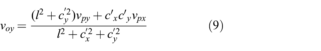
To relate the forces to object velocities, Lynch et al. (1992) used an ellipsoidal approximation to the limit surface. To simplify notation, we use subscript $b$ to refer to quantities associated with either the left $l$ or right $r$ boundary forces. Here, ${\mathbf{v}}_{o,b}$ and ${\omega }_{o,b}$ denote linear and angular object velocity, respectively. Here ${\mathbf{v}}_{p,b}$ are the push velocities that would create the boundary forces. They span the so-called “motion cone”:

$${\mathbf{v}}_{o,b}=\frac{{\omega }_{o,b}{l}^2}{m_b}{\mathbf{f}}_{\mathbf{b}}$$

(4)

$${\mathbf{v}}_{p,b}={\omega }_{o,b}(\frac{l^2}{m_b}{\mathbf{f}}_{\mathbf{b}}+\mathbf{k}\times \mathbf{c}\prime )$$

(5)

where ${\omega }_{o,b}$ acts as a scaling factor. As we are only interested in the direction of ${\mathbf{v}}_{p,b}$ and not in its magnitude, we set ${\omega }_{o,b}=m_b$ :

$${\mathbf{v}}_{p,b}=l^2{\mathbf{f}}_{\mathbf{b}}+m_b\mathbf{k}\times \mathbf{c}\prime$$

(6)

To compute the effective push velocity ${\mathbf{v}}_p$ , we need to determine the contact case: if the push velocity lies outside of the motion cone, the contact will slip. The resulting effective push velocity then acts in the direction of the boundary velocity ${\mathbf{v}}_{p,b}$ , which is closer to the push direction:

$${\mathbf{v}}_p=\frac{\mathbf{u}·\mathbf{n}}{{\mathbf{v}}_{p,b}·\mathbf{n}}{\mathbf{v}}_{p,b}$$

(7)

Otherwise, contact is sticking and we can use the pusher velocity as the effective push velocity ${\mathbf{v}}_p=\mathbf{u}$ . When the norm of $\mathbf{n}$ is zero (owing to, e.g., a wrong prediction of the perception neural network), we set the output ${\mathbf{v}}_{p,b}$ to zero.

The object will of course only move if the pusher is in contact with the object. To use the model also in cases where no force acts on the object, we introduce the contact indicator variable $s$ . It takes values between zero and one and is multiplied by ${\mathbf{v}}_p$ to switch off responses when there is no contact:

$${\mathbf{v}}_p=s{\mathbf{v}}_p$$

We allow $s$ to be continuous instead of binary to give the model a chance to react to the pusher making or breaking contact during the interaction.

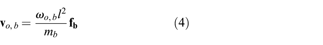
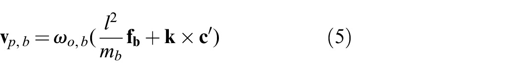
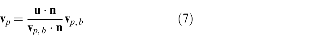
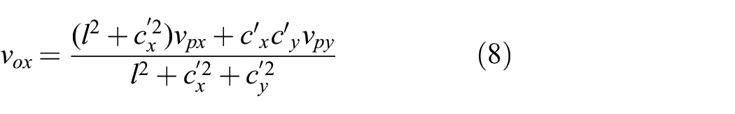
Stage 2: Using ${\mathbf{v}}_p$ to predict the object motion

Given the effective push velocity ${\mathbf{v}}_p$ and the contact point $\mathbf{c}\prime$ relative to the object center of mass, we can compute the linear and angular velocity ${\mathbf{v}}_o=[v_{\mathrm{ox}},v_{\mathrm{oy}},\omega ]$ of the object:

$$v_{\mathrm{ox}}=\frac{(l^2+c_x^{\prime 2})v_{\mathrm{px}}+{c\prime }_x{c\prime }_y{v}_{\mathrm{py}}}{l^2+c_x^{\prime 2}+c_y^{\prime 2}}$$

(8)

$$v_{\mathrm{oy}}=\frac{(l^2+c_y^{\prime 2})v_{\mathrm{py}}+{c\prime }_x{c\prime }_y{v}_{\mathrm{px}}}{l^2+c_x^{\prime 2}+c_y^{\prime 2}}$$

(9)

$$\omega =\frac{{c\prime }_x{v}_{\mathrm{oy}}-{c\prime }_y{v}_{\mathrm{ox}}}{l^2}$$

(10)

Discussion of underlying assumptions

The analytical model is built on three simplifying assumptions: (i) quasi- static pushing, i.e. the force applied to the object is large enough to move the object, but not to accelerate it; (ii) the pressure distribution of the object on the surface is uniform and the limit surface of frictional forces can be approximated by an ellipsoid; and (iii) the friction coefficient between surface and object is constant.

The analysis performed by Yu et al. (2016) shows that assumptions (ii) and (iii) are violated frequently by real-world data. Assumption (i) holds for push velocities less than 50 mm/s. In addition, the contact situation may change during pushing (as the pusher may slide along the object and even lose contact), such that the model predictions become increasingly inaccurate the longer ahead it needs to predict in one step.

3.2 Data

We use the MIT Push Dataset (Yu et al., 2016) for our experiments. It contains object pose and force recordings (not used here) from real robot experiments, where 11 different planar objects are pushed on 4 different surfaces. For each object–surface combination, the dataset contains about 6,000 pushes that vary in the manipulator (“pusher”) velocity and acceleration, the point on the object where the pusher makes contact and the angle between the object surface and the push direction. Pushes are 5 cm long and data was recorded at 250 Hz.

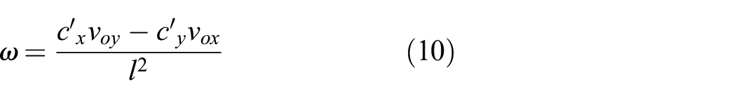
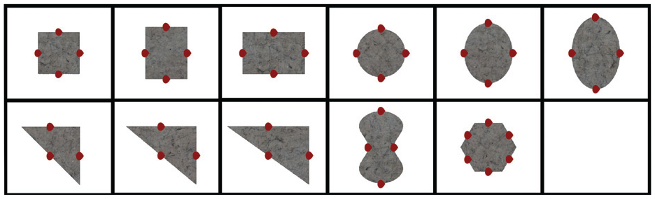
As this dataset does not contain RGB or depth images, we render them using OpenGL and the mesh data supplied with the dataset. In this work, we only use the depth images; RGB will be considered in future work. A rendered scene consists of a flat surface with one of four textures (representing the four surface materials), on which one of the objects is placed. The pusher is represented by a vertical cylinder with no arm attached. Figures 2 and 3 show the different objects and example images. We also annotated the dataset with all information necessary to apply the analytical model to use it as a baseline. The code for annotation and rendering is available at https://github.com/mcubelab/pdproc.

Fig. 2.

Rendered objects of the Push Dataset (Yu et al., 2016): rect1-3, ellip1-3, tri1-3, butter, hex. Red dots indicate the subset of contact points we use to collect a test set with held-out pushes for Experiment 5.4.

Fig. 3.

Rendered RGB and depth images on two of the four surfaces in the MIT dataset, plywood and abs.

For each experiment, we construct datasets for training and testing from a subset of the Push Dataset. As the analytical model does not take acceleration of the pusher into account, we only use push variants with zero pusher acceleration. However, we do evaluate on data with high pusher velocities, that break the quasi-static assumption made in the analytical model (in Section 5.5). One data point in our datasets consists of a depth image showing the scene before the push is applied, the object position before and after the push and the initial position and movement of the pusher. The prediction horizon is 0.5 seconds in all datasets. ¹ More information about the specific datasets for each experiment can be found in the corresponding sections.

We use data from multiple randomly chosen timesteps of each sequence in the Push Dataset. Some of the examples thus contain shorter push motions than others, as the pusher starts moving with some delay or ends its movement during the 0.5 second time window. To achieve more visual variance and to balance the number of examples per object type, we sample a number of transforms of the scene relative to the camera for each push. Finally, about a third of our dataset consists of examples where we moved the pusher away from the object, such that it is not affected by the push movement.

4 Combining neural networks and analytical models

We now introduce the neural network variants that we analyze in the following section. All architectures share the same first network stage that processes raw depth images and outputs a lower-dimensional encoding and the object position. Given this output, the pushing action (movement $\mathbf{u}$ and position $\mathbf{p}$ ) of the pusher, and the friction parameters $\mu$ and $l$ , ² the second part of these networks predicts the linear and angular velocity ${\mathbf{v}}_o$ of the object. This predictive part differs between the network variants. While three of them (simple, full, error) use variants of the analytical dynamics model established in Section 3.1, variant neural has to learn the dynamics with a neural network. The prediction part has about 1.8 million trainable parameters for all variants except for error, which has 2.7 million parameters.

We implement all our networks as well as the analytical model in tensorflow (Abadi et al., 2015), which allows us to propagate gradients through the analytical models just like any other layer.

4.1 Perception

The architecture of the network part that processes the image is depicted in Figure 4. We assume that the robot knows the position of its end-effector, which allows us to extract a small ( $80\times 80$ pixel) image patch (“glimpse”) around the tip of the pusher. If the pusher is close enough to the object to make contact, the important information for predicting the effect of the push, such as the contact point and the normal to the object surface, can be estimated from this smaller image. It thus serves as an attention mechanism to focus the computations on the most relevant part of the image. Only the position of the object needs to be estimated from the full image. The state representation that our perception model extracts thus contains the estimated object position and an encoding of the information represented in the glimpse.

Fig. 4.

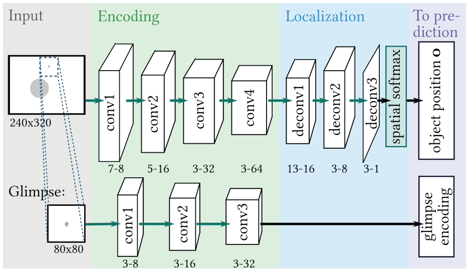
Perception part for all network variants. White boxes represent tensors, green arrows and boxes indicate network layers, whereas black arrows represent dataflow without processing. For green arrows, the type of layer (convolution or deconvolution) is denoted in the name of their output tensors. The numbers below the output tensors denote the kernel size and the number of output channels for each layer. The output of this module, glimpse encoding and the estimated object position $\mathbf{o}$ , serves as input for the prediction network depicted in Figure 5. For training, gradient information is backpropagated through the prediction to the perception network.

To obtain the glimpse encoding, we process the glimpse with three convolutional layers with ReLU nonlinearity, each followed by max-pooling and batch normalization (Ioffe and Szegedy, 2015). For estimating the object position, the full image is processed with a sequence of four convolutional and three deconvolution layers. The output of the last deconvolution has the same size as the image input and only has one channel that resembles an object segmentation map. We use spatial softmax (Levine et al., 2016) to calculate the pixel location of the segmented object center.

Initial experiments showed that not using the glimpse strongly decreased performance for all networks. We also found that using both the glimpse and an encoding of the full image for estimating all physical parameters was disadvantageous: using the full image increases the number of trainable parameters in the prediction network but adds no information that is not already contained in the glimpse.

4.2 Prediction

4.2.1 Neural network only (neural)

Figure 5(a) shows the prediction part of the variant neural, which uses a neural network to learn the dynamics of pushing. The input to this part is a concatenation of the output from perception with the action and friction parameter $l$ . The network processes this input with three fully connected layers before predicting the object velocity ${\mathbf{v}}_o$ . All intermediate fully connected layers use ReLU nonlinearities. The output layers do not apply a nonlinearity.

Fig. 5.

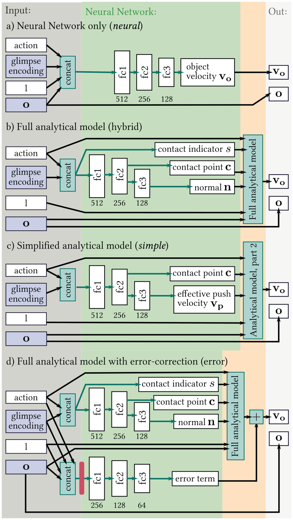
Prediction parts of the four network variants neural, hybrid, simple, and error. White and purple boxes represent tensors, where the purple color indicates tensors that are computed by the perception part shown in Figure 4. During training, the gradient information is backpropagated through these tensors to the perception part. Green arrows and boxes indicate network layers, whereas black arrows represent dataflow without processing. In this network, all green arrows represent fully connected layers and the numbers beneath their output tensors (fc) denote the number of output channels. The red bar in architecture (d) indicates that no gradients are propagated to the inputs of this layer.

4.2.2 Full analytical model (hybrid)

This variant uses the complete analytical model as described in Section 3.1. Several fully connected layers extract the necessary input values from the glimpse encoding and the action, as shown in Figure 5(b). These are the contact point $\mathbf{c}$ , the surface normal $\mathbf{n}$ , and the contact indicator $s$ . For predicting $s$ , we use a sigmoidal nonlinearity to limit the predicted values to $[0,1]$ .

4.2.3 Simplified analytical model (simple)

Simple (Figure 5(c)) only uses the second stage of the analytical model. As for hybrid, a neural network extracts the model inputs (effective push velocity ${\mathbf{v}}_p$ , contact point $\mathbf{c}$ ) from the encoded glimpse and the action.

We use this variant as a middle ground between the two other options: it still contains the main mechanics of how an effective push at the contact point moves the object, but leaves it to the neural network to deduce the effective push velocity from the scene and the action. This gives the model more freedom to correct for possible shortcomings of the analytical model. We expect these to manifest mostly in the first stage of the model, as small errors can have a large effect there when they influence whether a contact is estimated as sticking or slipping. As the second stage of the analytical model does not specify how the input action relates to the object movement, simple also allows us to evaluate the importance of this particular aspect of the analytical model.

4.2.4 Full analytical model + error term (error)

One concern when using a predefined analytical model is that the trained network cannot improve over the performance of the analytical model. If the analytical model is inaccurate, the hybrid architecture can only compensate to some degree by manipulating the input values of the model, i.e., by predicting “incorrect” values for the components of the state representation. This limits its ability to compensate for model errors as it might not be possible to account for all types of errors in this way.

As an alternative, we propose to learn an error-correction term that is added to the output prediction of the analytical model. The error term is thus not constrained by the model and should be able to compensate for a broader class of model errors.

Figure 5(d) shows the architecture. As input for predicting the error term, we use the same values that neural receives for predicting the object velocity, i.e., the glimpse encoding, the action, the predicted object position, and the friction parameter. Note that we do not propagate gradients to the inputs of the error-prediction module. The intuition behind this is that we do not want the error prediction to interfere with the prediction of the inputs for the analytical model. We evaluate the effect of this architectural decision in Section 5.8. A second variant that we compare to in this section aims to improve the generalizability of the error prediction to faster push movements. This is achieved by normalizing the input action to unit length before feeding it into the error-prediction module.

4.3 Training

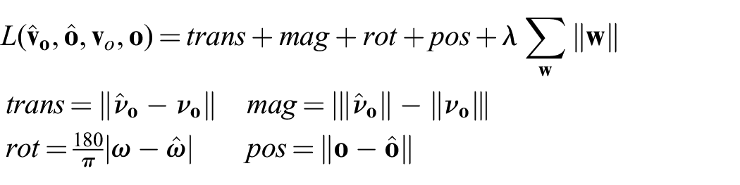
All our architectures are trained end-to-end, i.e., the loss is propagated through the prediction to the perception part of the networks. The loss $L$ penalizes the Euclidean distance between the predicted and the real object position in the input image (pos), the Euclidean error of the predicted object translation (trans), the error in the magnitude of translation (mag) and in angular movement (rot) in degrees (instead of radians, to ensure that all components of the loss have the same order of magnitude). We use weight decay with $\lambda =0.001$ .

Let ${\hat{\mathbf{v}}}_{\mathbf{o}}$ and $\hat{\mathbf{o}}$ denote the predicted and ${\mathbf{v}}_o$ , $\mathbf{o}$ the real object movement and position. $\mathbf{w}$ are the network weights and ${\nu }_{\mathbf{o}}=[v_{\mathrm{ox}},v_{\mathrm{oy}}]$ denotes linear object velocity:

$$\begin{array}{c}L({\hat{\mathbf{v}}}_{\mathbf{o}},\hat{\mathbf{o}},{\mathbf{v}}_o,\mathbf{o})=\mathrm{trans}+\mathrm{mag}+\mathrm{rot}+\mathrm{pos}+\lambda \sum _{\mathbf{w}}\Vert \mathbf{w}\Vert \hfill \\ \begin{array}{cc}\mathrm{trans}=\Vert {\hat{\nu }}_{\mathbf{o}}-{\nu }_{\mathbf{o}}\Vert \hfill & \mathrm{mag}=|\Vert {\hat{\nu }}_{\mathbf{o}}\Vert -\Vert {\nu }_{\mathbf{o}}\Vert |\hfill \\ \multicolumn{1}{c}{\mathrm{rot}=\frac{180}{\pi }|\omega -\hat{\omega }|}& \mathrm{pos}=\Vert \mathbf{o}-\hat{\mathbf{o}}\Vert \hfill \end{array}\hfill \end{array}$$

When using the variant hybrid, a major challenge is the contact indicator $s$ : in the beginning of training, the direction of the predicted object movement is mostly wrong. Therefore, $s$ receives a strong negative gradient, causing it to decrease quickly. As the predicted motion is effectively multiplied by $s$ , a low $s$ results in the other parts of the network receiving small gradients and thus greatly slows down training. We therefore add the error in the magnitude of the predicted velocity to the loss to prevent $s$ from decreasing too far in the early training phase.

We use Adam optimizer (Kingma and Ba, 2014) with a learning rate of $0.0001$ and a batch-size of 32 for 75,000 steps.

5 Evaluating generalization

In this section, we test our hypothesis that using an analytical model for prediction together with a neural network for perception improves data efficiency and leads to better generalization than using neural networks for both, perception and prediction. We evaluate how the performance of the networks depends on the amount of training data (Experiment 5.3) and how well they generalize to (i) pushes with new pushing angles and contact points (Experiment 5.4), (ii) new push velocities (Experiment 5.5), and (iii) unseen objects (Experiment 5.6).

For the experiments in this section, we use a top-down view of the scene, such that the object can only move in the image plane and the $z$ -coordinate of all scene components remains constant. This simplifies the application of the analytical model by removing the need for an additional transform between the camera and the table. It also simplifies the perception task and allows us to focus this evaluation on the comparison of the hybrid and the purely neural approach. In Section 6, we show how to extend the proposed model to work on more difficult camera settings.

5.1 Baselines

We use three baselines in our experiments. All of them use the ground-truth input values of the analytical model (action, object position, contact point, surface normal, contact indicator, and friction coefficients) instead of depth images. They, thus, do not solve the full problem of predicting object movement from raw sensory input. Instead, they address the easier problem of prediction given perfect state information. Accordingly, the baselines only output the object velocity, but not its initial position in the scene.

If the pusher makes contact with the object during the push, but is not in contact initially, we use the contact point and normal from when contact is first made and shorten the action accordingly. Note that this gives the baseline models an additional advantage over architectures that have to infer such input values from raw sensory data.

The first baseline is just the average translation and rotation over the dataset. This is equal to the error when always predicting zero movement, and we therefore name it zero. The second, physics, is the full analytical model evaluated on the ground-truth input values. The third baseline, called neural dyn, is a neural network that has the same three-layer architecture as the prediction module of neural (see Figure 5(a) for details). The difference between neural and neural dyn is their input: While neural receives the glimpse encoding and object position from the perception network as input, neural dyn receives the ground-truth physical state representation that is also used in the analytical model. This allows us to evaluate whether neural benefits from being able to learn its own state representation (the glimpse encoding) end-to-end through the prediction part.

5.2 Metrics

For evaluation, we compute the average Euclidean distance between the predicted and the ground-truth object translation (trans) and position (pos) in millimeters as well as the average error on object rotation (rot) in degrees. As our datasets differ in the overall object movement, we report errors on translation and rotation normalized by the average motion in the corresponding dataset given by the error of the baseline zero.

5.3 Data efficiency

The first hypothesis we test is that combining the analytical model with a neural network for perception reduces the required training data as compared with a pure neural network.

5.3.1 Data

We use a dataset that contains all objects from the MIT Push dataset and all pushes with velocity 20 mm/s and split it randomly into training and test set. This results in about 190,000 training examples and about 38,000 examples for testing. To evaluate how the networks’ performance develops with the amount of training data, we train the models on different subsets of the training split with sizes from 2,500 to the full 190,000. We always evaluate on the full test split. To reduce the influence of dataset composition, especially on the small datasets, we average results over multiple different datasets with the same size.

5.3.2 Results

Figure 6 shows how the errors in predicted translation, rotation and object position develop with more training data and Table 1 contains numeric values for training on the biggest and smallest training split. As expected, the combined approach of neural network and analytical model (hybrid and error) already performs very well on the smallest dataset (2,500 examples) and beats the other models including the neural dyn baseline, which uses the ground-truth state representation, by a large margin. It takes more than 20,000 training examples for the other models to reach the performance of hybrid, where predicting rotation seems to be harder to learn than translation.

Fig. 6.

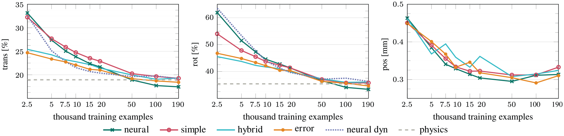
Prediction errors versus training set size ( $x$ -axis in logarithmic scale). Errors on translation and rotation are given as percentage of the average movement in the test set. The model-based architecture hybrid performs much better than the other networks when training data is sparse.

Table 1.

Error in predicted translation (trans) and rotation (rot) as a percentage of the average movement given by zero (standard errors in brackets). pos denotes the error in predicted object position. Values shown are for training on the full training set (190,000 examples) and on a 2,500 examples subset.

		trans (%)	rot (%)	pos (mm)
2,500	neural	$33.6(0.18)$	$62.54(0.42)$	$0.46(0.002)$
	simple	$32.3(0.19)$	$53.6(0.37)$	$0\mathbf{.}44\mathbf{(}0\mathbf{.}002\mathbf{)}$
	hybrid	$25.4(0.17)$	$45\mathbf{.}5\mathbf{(}0\mathbf{.}36\mathbf{)}$	$0.46(0.002)$
	error	$24\mathbf{.}7\mathbf{(}0\mathbf{.}16\mathbf{)}$	$46.8(0.36)$	$0.45(0.002)$
	neural dyn	$32.6(0.19)$	$63.5(0.46)$	—
19,000	neural	$17\mathbf{.}4\mathbf{(}0\mathbf{.}12\mathbf{)}$	$33\mathbf{.}4\mathbf{(}0\mathbf{.}28\mathbf{)}$	$0\mathbf{.}31\mathbf{(}0\mathbf{.}002\mathbf{)}$
	simple	$19.3(0.13)$	$35.7(0.3)$	$0.33(0.002)$
	hybrid	$19.3(0.13)$	$36.1(0.3)$	$0.32(0.002)$
	error	$18.4(0.12)$	$34.6(0.29)$	$0\mathbf{.}31\mathbf{(}0\mathbf{.}002\mathbf{)}$
	neural dyn	$19.2(0.12)$	$36.3(0.29)$	—
	physics	$18.95(0.13)$	$35.4(0.3)$	—
	zero	$2.95(0.02)$ mm	$1.9(0.01)°$	—

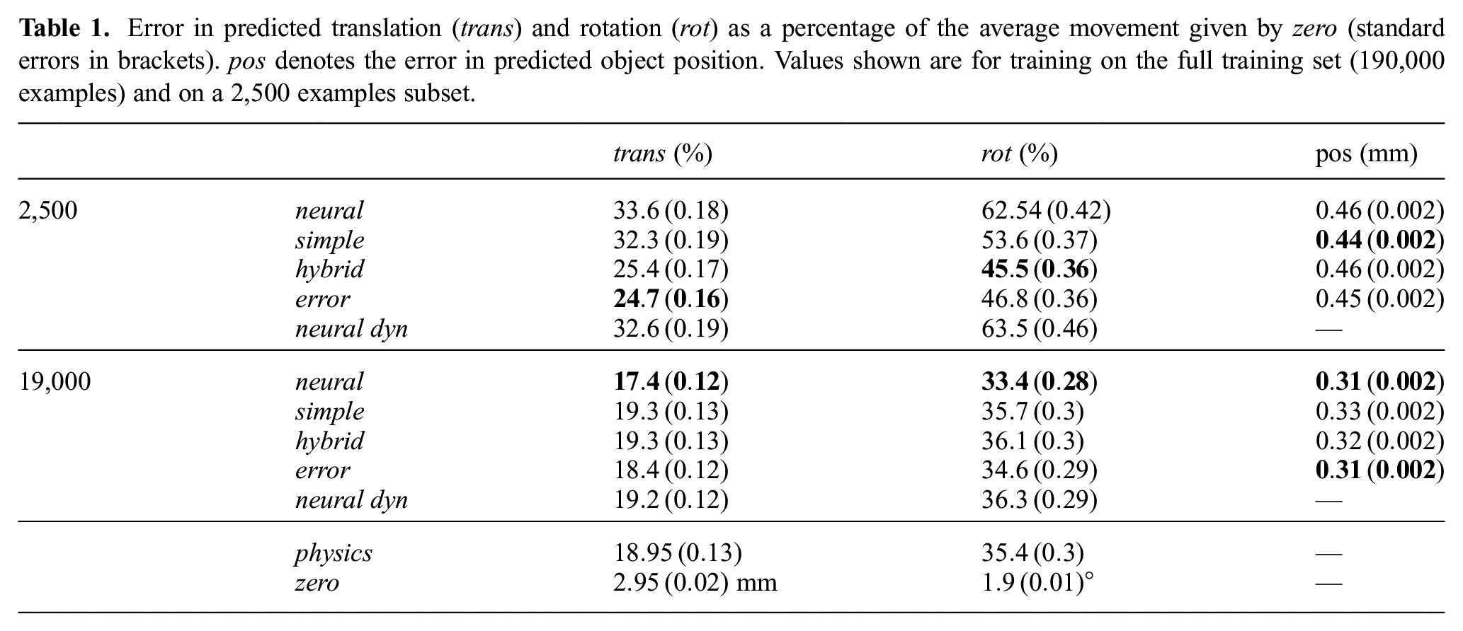
Despite of having to rely on raw depth images instead of the ground-truth state representation, all models perform at least close to the physics baseline when using the full training set. However, only the pure neural network and the hybrid model with error correction are able to improve on the baseline. This shows that the analytical model limits hybrid in fitting the training data perfectly, since the model itself is not perfect and does not allow for overfitting to noise in the training data. Neural and error have more freedom for fitting the training distribution, which however also increases the risk of overfitting.

Combining the learned error correction with the fixed analytical model is especially helpful for predicting the translation of the object. To also improve the prediction of rotations, the model needs more than 20,000 training examples, which is similar to neural. While neural makes a larger improvement on the full dataset, error combines the comparably good performance of hybrid on few training examples with the ability to improve on the model given enough data.

The variant simple, which uses only the second part of the analytical model, also combines learning and a fixed model for predicting the dynamics. However, in contrast to error, this variant seems to combine the disadvantages of both approaches: it needs much more training data than hybrid, but is still limited by the performance of the analytical model and is quickly outperformed by the pure neural network when more data is available.

The comparison of neural and the baseline neural dyn shows that despite having access to the ground-truth data, neural dyn actually performs worse than neural on the full dataset. This seems to agree with the theory of Agrawal et al. (2016), that training perception and prediction end-to-end and letting the network chose its own state representation instead of forcing it to use a predefined state may be beneficial for neural learning.

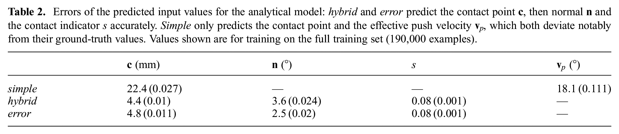
Finally, we evaluate how accurate the predicted input values to the analytical model are for simple, hybrid, and error. If the analytical model was perfect, we would expect the predicted values to be very close to the real physical state. Higher errors could, thus, indicate that the models learn to compensate for inaccuracies of the analytical model.

As can be seen in Table 2, both hybrid and error make fairly accurate predictions for the object state, with contact point errors around 5 mm and less than 5° angle between the predicted and correct normal. The contact point indicator $s$ is also estimated with high accuracy. Only variant simple shows a larger error between the predicted and true contact points. The predicted effective push velocity ${\mathbf{v}}_p$ also does not match the values we obtained from applying the first stage of the analytical model on ground-truth input very closely. As these errors do not seem to harm the overall prediction accuracy, we conclude that they cancel each other out. This shows that simple is not as strongly constrained by its analytical component as hybrid and error and that it thus has more freedom in choosing its state representation.

Table 2.

Errors of the predicted input values for the analytical model: hybrid and error predict the contact point $\mathbf{c}$ , then normal $\mathbf{n}$ and the contact indicator $s$ accurately. Simple only predicts the contact point and the effective push velocity ${\mathbf{v}}_p$ , which both deviate notably from their ground-truth values. Values shown are for training on the full training set (190,000 examples).

	$\mathbf{c}$ (mm)	$\mathbf{n}$ (°)	$s$	${\mathbf{v}}_p$ (°)
simple	$22.4(0.027)$	—	—	$18.1(0.111)$
hybrid	$4.4(0.01)$	$3.6(0.024)$	$0.08(0.001)$	—
error	$4.8(0.011)$	$2.5(0.02)$	$0.08(0.001)$	—

5.3.3 Summary

All our models reach the performance of the (perception-free) physics baseline given enough training data. Combining neural networks and analytical models strongly improves performance in comparison with purely learned models when little training data is available. However, neural can achieve the highest prediction accuracy and beat the physics baseline when trained on a very large dataset.

To further improve the prediction accuracy of hybrid while preserving its data efficiency, an additive error-correction term can be learned. Replacing a part of the analytical model with a learned component in simple in contrast harmed the data efficiency.

5.4 Generalization to new pushing angles and contact points

The previous experiment showed the performance of the different models when testing on a dataset with a very similar distribution to the training set. Here, we evaluate the performance of the networks on held-out push configurations that were not part of the training data. Note that while the test set contains combinations of object pose and push action that the networks have not encountered during training, the pushing actions or object poses themselves do not lie outside of the value range of the training data. This experiment thus test the models’interpolation abilities.

5.4.1 Data

We again train the networks on a dataset that contains all objects and pushes with velocity $20$ mm/s. For constructing the test set, we collect all pushes with (i) pushing angles $\pm 20°$ and $0°$ to the surface normal (independent from the contact points) and (ii) at a set of contact points illustrated in Figure 2 (independent of the pushing angle).

The remaining pushes are split randomly into a training and a validation set, which we use to monitor the training process. There are about 114,000 data points in the training split, 23,000 in the validation split, and 91,000 in the test set.

5.4.2 Results

As Table 3 shows, hybrid and error perform best for predicting the object velocity for pushes that were not part of the training set. Although still being close, none of the networks can outperform the physics baseline on this test set.

Table 3.

Prediction errors for testing on pushes with pushing angles and contact points not seen during training

	trans (%)	rot (%)	pos (mm)
neural	$16.5(0.06)$	$36.1(0.17)$	$0.31(0.001)$
simple	$16.4(0.06)$	$37.1(0.18)$	$0\mathbf{.}31\mathbf{(}0\mathbf{.}001\mathbf{)}$
hybrid	$15\mathbf{.}6\mathbf{(}0\mathbf{.}07\mathbf{)}$	$35.3(0.19)$	$0.31(0.001)$
error	$15\mathbf{.}6\mathbf{(}0\mathbf{.}07\mathbf{)}$	$34\mathbf{.}5\mathbf{(}0\mathbf{.}18\mathbf{)}$	$0.32(0.001)$
neural dyn	$18.1(0.07)$	$44.1(0.2)$	—
physics	$14.6(0.06)$	$32.8(0.18)$	—
zero	$4.36(0.013)$ mm	$2.27(0.009)°$	—

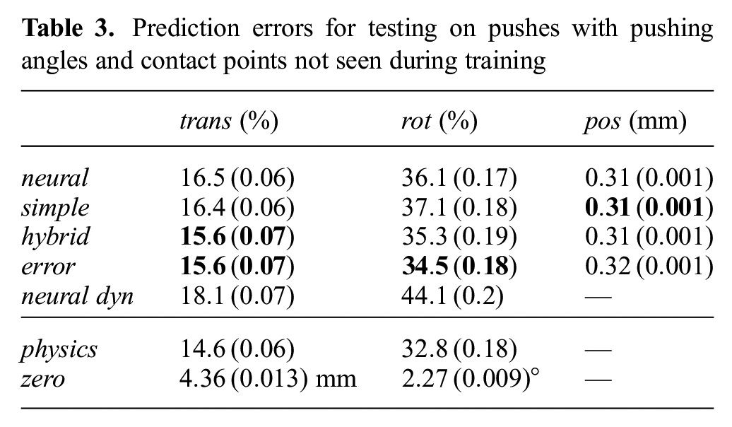
Note that the difficulty of the test set in this experiment differs from that in the previous experiment, as can be seen from the different performance of the physics baseline: owing to the central contact point locations and small pushing angles, the test set contains a high proportion of pushes with sticking contact (see Section 3.1), for which the resulting object movement is similar to the pusher movement. Prediction in sticking contact cases is therefore generally simpler than in cases in which the pusher slides along the object. This difference in difficulty makes it hard to compare the results between Tables 1 and 3 in terms of absolute values.

With more than 100,000 training examples, we supply enough data for the pure neural model to clearly outperform the combined approach and the baseline in the previous experiment (i.e., when the test set is similar to the training set, see Figure 6). The fact that neural now performs worse than hybrid and physics indicates that its advantage over the physics baseline may not come from it learning a more accurate dynamics model. Instead, it probably memorizes specific input–output combinations that the analytical model cannot predict as well, e.g., owing to noisy object pose data.

This might also be the reason why error cannot improve on hybrid as much as in the previous experiment, especially when it comes to predicting the translation of the object. It is however encouraging to see that the learned error correction term for the predicted rotation is still beneficial for pushes not seen during training.

In contrast to hybrid and error, simple again does not seem to profit from using the simplified analytical model and performs similar to neural.

As in the previous experiment (see Table 1), we also tested the generalization ability of the networks when trained on a smaller training set. If we supply only 2,500 training examples, the difference between hybrid and the purely learned model is again much more pronounced: hybrid achieves 20.3% translation and 43.8% rotation error whereas neural lies at 38.7% and 63.4%, respectively.

5.4.3 Summary

The purely learned model performs worse than the hybrid approaches when interpolating to unseen push configurations. For all models, the difference to the physics baseline is larger when the training distribution does not match the test distribution.

5.5 Generalization to different push velocities

In this experiment, we test how well the networks generalize to unseen push velocities. In contrast to the previous experiment, the test actions in this experiment have a different value range than the actions in the training data, and we are thus looking at extrapolation. As neural networks are usually not good at extrapolating beyond their training domain, we expect the model-based network variants to generalize better to push velocities not seen during training.

5.5.1 Data

We use the networks that were trained in the first experiment (Section 5.3) on the full (190,000) training set. The push velocity in the training set is thus 20 mm/s. We evaluate on datasets with different push velocities ranging from 10 to 300 mm/s. Since seeing only one push velocity during training might be a disadvantage for the learned models, we also compose two new training datasets, one with velocities conform to the quasi-static assumption (10 and 20 mm/s) and one with a higher second velocity (20 and 50 mm/s) that violates the quasi-static assumption. Both datasets have slightly more than 125,000 training examples.

5.5.2 Results

Results are shown in Figure 7. As the input action does not influence perception of the object position, we only report the errors on the predicted object motion.

Fig. 7.

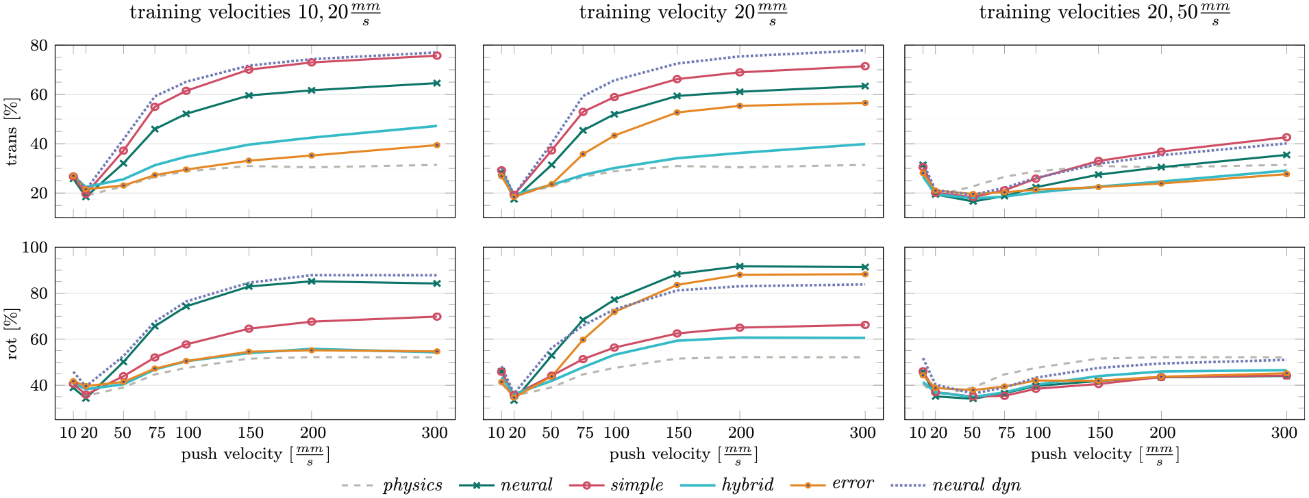
Errors on predicted translation and rotation for testing on different push velocities. In the first column, all models were trained on push velocities 10 and 20 mm/s, in the second column on velocity 20 mm/s and in the last column on velocities 20 and 50 mm/s. When training on velocities that are small enough to ensure quasi-static pushing, all models have trouble extrapolating to higher velocities, but hybrid and error stay much closer to the physics baseline than simple, neural, and neural dyn. Seeing additional training data from a higher push velocity (50 mm/s) that violates the quasi-static assumption strongly improves the generalization to higher velocities for all models and enables them to beat the physics baseline in many cases. In particular, for the predicted object translation, we however still see a much stronger decrease in performance for simple, neural, and neural dyn than for hybrid, error, and physics.

When training on push velocities below 50 mm/s, we see a very large difference between the performance of our combined approach and the pure neural network for higher velocities. The predictions of neural and neural dyn quickly become very inaccurate, with the error on predicted translation rising to more than 60% and the error on predicted rotation to more than 80% of the error when predicting zero movement always. The performance of hybrid, on the other hand, is most constant over the different push velocities and declines only slightly more than the physics baseline. Error also extrapolates well, but only when trained on more than one push velocity.

Like neural and neural dyn, simple also performs worse on higher velocities. Its performance when predicting rotations, however, degrades much less than for predicting translations. The reason for this is that all three architectures struggle mostly with predicting the correct magnitude of the object translation and not so much with predicting the translation’s direction. By using the second stage of the analytical model, simple has information about how the direction of the object translation and the contact point relate to its rotation, which results in much more accurate predictions.

The advantage of hybrid for extrapolation lies in the first stage of the analytical model, which allows it to scale its predictions according to the magnitude of the action and the contact indicator $s$ . Both are, in essence, multiplication operations. A general multiplication of inputs cannot, however, be expressed using only fully connected layers (as used by simple, neural, neural dyn, and the error-prediction part of error) because fully connected layers essentially perform weighted additions of their inputs. Thus, instead of learning the underlying function, the networks are forced to resort to memorizing input–output relations for the magnitude of the object motion, which explains why extrapolation does not work well, especially when training on low push velocities.

When combining the prediction of the analytical model with a learned error-term and training only on one push velocity, the resulting model suffers from the same issues as the other network-based variants. The decline is, however, less pronounced than for neural, and only starts after $50$ mm/s. A possible reason for this is that the error-correction term is rather small compared with the output of the analytical model. This means that the weights with which the action enters the computation of the error term are smaller than for neural, simple, or neural dyn.

Interestingly, adding a second training velocity completely changes the picture and makes error perform on par with or even better than hybrid. Our hypothesis is that seeing different velocities during training prevents the error term from overfitting to the input action and minimizes the effect of the action magnitude on the predicted error-term. In Section 5.8, we show that for training on only one push velocity, error can also be made more robust to higher velocities by normalizing the push action before using it as input to the error prediction.

While the physics baseline performs better than the models trained on low push velocities, it predictions also get worse on higher push velocities. The main reason for this is that the quasi-static assumption of the model is violated: for pushes faster than 20 mm/s, the object is accelerated and can continue sliding even after contact to the pusher was lost.

How different the dynamics of pushing are between the quasi-static and this dynamic behavior also becomes apparent when we include the push velocity 50 mm/s in the training data for our learned models: they all extrapolate much better to higher velocities and are often able to outperform the physics baseline. This increase of performance for fast pushes, however, only extends to the slowest push velocity (10 mm/s) for hybrid, whereas all other models perform slightly worse than their counterparts that were only trained on one push velocity.

We also still see that with increasing push velocities, the variants simple, neural, and neural dyn make significantly larger errors for predicting the translation of the object than hybrid and error. Interestingly, for predicting the object rotation, all models except for neural dyn perform extremely well, with hybrid even doing slightly worse than the others. A possible reason for this difference between translation and rotation could be that the magnitude of rotations does not increase as strongly with the push velocity as the magnitude of translations: the average rotation increases from 1.4° on 10 mm/s pushes to 14.4° on 300 mm/s pushes, whereas translation increases from 2.1 to 24.8 mm. The models therefore need to change their predicted rotations less in response to higher push velocities than they have to for translation.

5.5.3 Summary

Extrapolating to different push velocities is difficult for purely learned models, especially when the training data only contains low pushing velocities. Using the analytical model in hybrid and error facilitates extrapolation by providing multiplication operations and explaining the influence of the action on the resulting movement. As the quasi-static assumption of the analytical model is violated by fast pushes, our models can, however, learn to outperform the physics baseline in this regime when they have training data from faster pushes.

5.6 Generalization to different objects

This experiment tests how well the networks generalize to unseen object shapes and how many different objects the networks have to see during training to generalize well.

5.6.1 Data

We train the networks on three different datasets: with one object (butter), two objects (butter and hex), and three objects (butter, hex, and one of the ellipses or triangles). The datasets with fewer objects contain more augmented data, such that the total number of data points is about 35,000 training examples in each. As test sets, we use one dataset containing the three ellipses and one containing all triangles. While this is fewer training data than in the previous experiments, it should be sufficient for the pure neural network to perform as well as hybrid, since the test sets contain only few objects.

5.6.2 Results

The results in Figure 8 show that neural is consistently worse than the other networks when predicting rotations. It also improves most notably when one example of the test objects is in the training set. The differences between the models are less pronounced when predicting translation, except for simple, which performs particularly bad on triangles. The different models do not differ much when predicting position, which is not surprising, since they share the same perception architecture. The architecture with added error term does not perform very different from hybrid, which implies that the error-correction term does not depend much on the shape of the object.

Fig. 8.

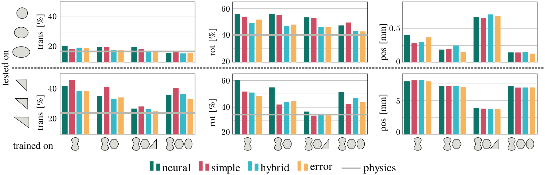
Prediction errors in translation, rotation, and position on objects not seen during training. Training objects are shown on the $x$ -axis. The top row shows results for evaluating on ellipses, the bottom row on triangles. All networks generalize well to ellipses, but are worse for triangles, where the error in predicted position is by a factor of 10 higher than for the other objects. Neural particularly struggles with predicting rotations of previously unseen objects.

In general, all models perform surprisingly well on ellipses, even if the models only had access to data from the butter object. Reaching the baseline performance on triangles is, however, only possible with a triangle in the training set. Predicting the object’s position is most sensitive to the shapes seen during training: it generalizes well to ellipses that have similar shape and size as the butter or hex object. The triangles, on the other hand, are very different from the other objects in the dataset and the error for localizing triangles is a factor of 10 higher than for ellipses.

5.6.3 Summary

Using the analytical model in hybrid and error also facilitates generalization to novel object shapes, which is more difficult for the purely learned model. All models struggle slightly with localizing objects of unknown shapes.

5.7 Visualizations

As a qualitative evaluation, we plot the predictions of our networks, the physics and neural dyn baselines and the ground-truth object motion for 200 repetitions of the same push configuration. The data for these repeated pushes is available with the MIT Push dataset. All repetitions have the same nominal pushing angle ( $0°$ ), velocity ( $20$ mm/s), and contact point, but the exact values vary slightly between individual pushes. To keep the visual input diverse, we also sample a different transformation of the whole scene for each repetition, such that the object’s pose in the image varies. The networks were trained on the full dataset from Experiment 5.3.

The results shown in Figure 9 illustrate that the resulting ground-truth object motion for the same push configuration varies greatly between trials. In particular, in terms of object rotation, the distribution of outcomes shows two distinct modes (one close to the overall mean and one with notably stronger object rotation). By comparing the ground truth with the prediction of the analytical model, we can estimate how much of this variance is due to slight changes in the push configuration between trials (these also reflect in the analytical model) and how much is caused by other, non-deterministic effects.

Fig. 9.

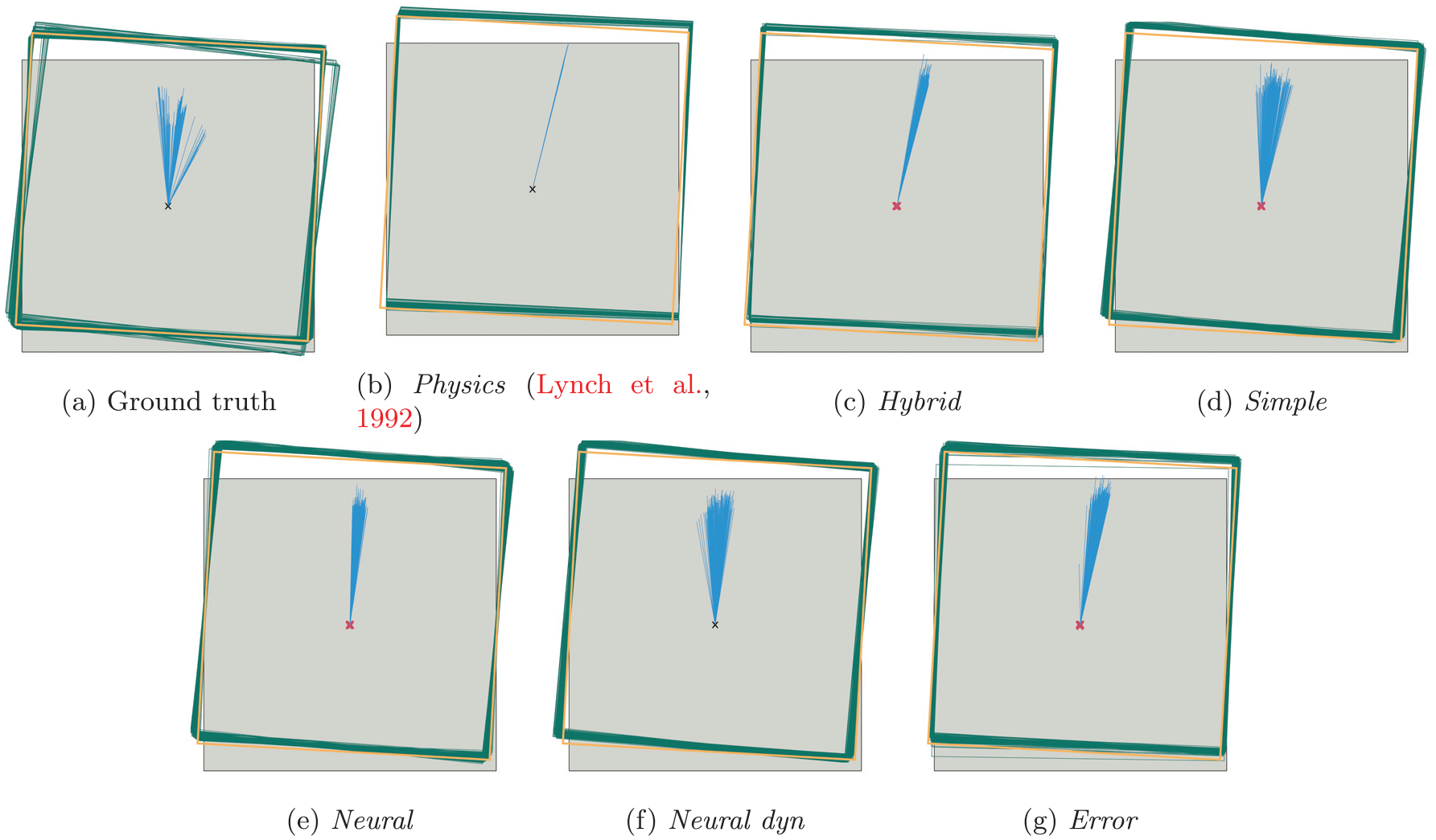
Qualitative evaluation on 200 repeated pushes with the same push configuration (angle, velocity, contact point). The green rectangles show the (predicted) pose of the object after the push and the blue lines illustrate the object’s translation (for better visibility, we upscaled the lines by a factor of five). The thicker orange rectangle is the average ground-truth pose of the object after the push. Red crosses indicate the predicted initial object positions. All models predict the movement of the object and its initial position well, but cannot capture the multimodal distribution of the ground-truth data.

The predictions of hybrid and the analytical model are very similar. This again shows that the state representation that the neural network part of hybrid predicts is mostly accurate. The plotted contact point and normal estimates in Figure 10 further confirm this. Adding an error-correction term to the hybrid architecture improves the average estimation quality a little, but also increases the variance of the predictions.

Fig. 10.

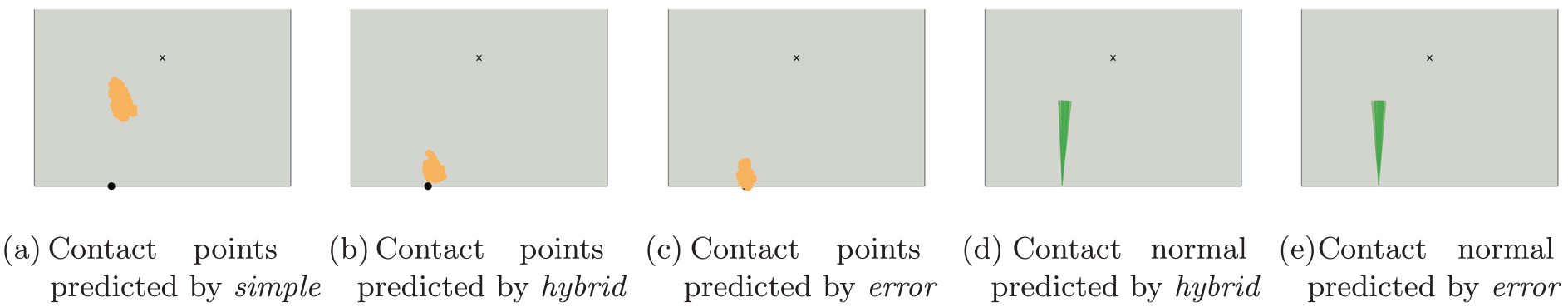
Predicted contact points and normals from 200 repeated pushes with the same push configuration (angle, velocity, contact point). The black point marks the (average) ground-truth contact point. While hybrid and error make fairly accurate predictions, simple predicts the contact points not on the edge of the object, but close to its center.

The visualizations for the other models (Figure 9(d)–(f)) show that they also make good predictions in this example, but simple and neural dyn have much more variance in the direction of the predicted translation than hybrid or neural. It is also interesting to see that neural, neural dyn, and simple all slightly overestimate the object rotation in comparison with the mean ground-truth movement, whereas physics slightly underestimates it. Figure 10 also shows that simple is not very accurate in predicting the contact points, confirming the quantitative results found in Table 2. As stated previously, we believe that this inaccuracy is compensated for by the predicted ${\mathbf{v}}_p$ .

5.8 Evaluation of the error architecture

The previous results have shown that adding a learned error-correction term to the output of the analytical model in the hybrid architecture enables the network to improve over the performance of the analytical model. The error model we analyzed is able to outperform hybrid and the physics baseline if the training set and the test set are similar (see Experiment 5.3).

In the following experiments, we evaluate different choices we made for the architecture of error. We also compare the ability of hybrid and error to compensate for larger errors in the analytical model.

5.8.1 Evaluation of different architectures

As explained in Section 4, we chose to block the propagation of gradients from the error-correction module to the glimpse encoding, because we did not want the error computation to interfere with the prediction of the state representation. Here, we also evaluate an architecture err-grad that does not block the gradient propagation. This architecture manages to beat hybrid by an even bigger margin, as listed in Table 4.

Table 4.

Evaluation of different architectures for predicting an error-correction term. In contrast to error, error-grad allows the propagation of gradients from the error-prediction module to the glimpse encoding. Error-norm instead normalizes the push action to unit length before using it as input to the error prediction. Values shown are for training on the full training set (190,000 examples). Results for hybrid and neural are repeated for reference.

	trans (%)	rot (%)	pos (mm)
Neural	$17\mathbf{.}4\mathbf{(}0\mathbf{.}12\mathbf{)}$	$33\mathbf{.}4\mathbf{(}0\mathbf{.}28\mathbf{)}$	$0.31(0.002)$
hybrid	$19.3(0.13)$	$36.1(0.3)$	$0.32(0.002)$
error	$18.4(0.12)$	$34.6(0.29)$	$0.31(0.002)$
error-grad	$17.9(0.12)$	$34.4(0.29)$	$0\mathbf{.}29\mathbf{(}0\mathbf{.}002\mathbf{)}$
error-norm	$18.3(0.12)$	$35.3(0.29)$	$0.31(0.002)$
physics	$18.95(0.13)$	$35.4(0.3)$	—
zero	$2.95(0.02)$ mm	$1.9(0.01)°$	—

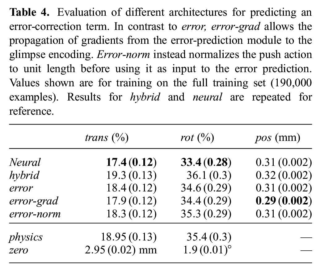
The downside of propagating the gradients becomes apparent if we look at generalization to new pushing velocities: while the predictions of error become worse with increasing velocity, they still remain more accurate than the predictions of neural, as illustrated in Figure 11. Error-grad on the other hand performs even worse than the pure neural network. A reason for this difference could be that error-grad relies more strongly on the error-correction term than error. This allows it to fit the training data more closely but at the same time impedes generalization to novel actions.

Fig. 11.

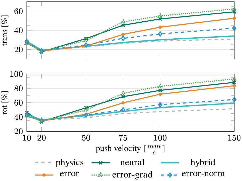
Evaluation of the different architectures for predicting an error-correction term on unseen push velocities. All models were trained on push velocity 20 mm/s. None of the error-prediction models is as robust as hybrid to higher input velocities. Error-norm performs best because its predicted error terms are independent of the push velocity. Error-grad presumably relies more on the error-prediction term than the other architectures and, therefore, performs worst outside of the training domain.

As explained previously, the reason for the decline in performance when extrapolating is that the neural networks cannot scale their predictions correctly according to the input velocity. One possibility to make the error prediction more robust to higher input velocities is the architecture we call error-norm. In this model, we scale the push action to unit length before using it as input to the error prediction. This makes the error prediction independent of the magnitude of the action, while still giving it information about the push direction. The resulting model performs only slightly worse than error inside the training domain, but much better for extrapolation. It is still worse than hybrid though, as it cannot properly adapt the error-term to match higher velocities.

5.8.2 Compensation of model errors

Using the error-correction term of course becomes much more interesting if the analytical model is bad. To test how well the hybrid and error architectures can compensate for wrong models, we manipulate the friction parameter $l$ by setting it to 1.5 or 3 times its real value. The results are listed in Table 5.

Table 5.

Prediction errors of physics, hybrid, and error when using a manipulated friction parameter $l$ . In contrast to physics, both neural networks can compensate for the resulting error of the analytical model. Hybrid can, however, only modify the input values to the analytical model, while error can correct the model’s output directly and, thus, compensates for the error of the analytical model much better.

	trans (%)	rot (%)	pos (mm)
$1.5·l$
hybrid	$20.7(0.13)$	$40.5(0.32)$	$0.3(0.002)$
error	$19\mathbf{.}2\mathbf{(}0\mathbf{.}14\mathbf{)}$	$35\mathbf{.}9\mathbf{(}0\mathbf{.}3\mathbf{)}$	$0\mathbf{.}25\mathbf{(}0\mathbf{.}002\mathbf{)}$
physics	$23.9(0.15)$	$46.1(0.37)$	—
$3·l$
hybrid	$25.1(0.15)$	$66.9(0.45)$	$0\mathbf{.}31\mathbf{(}0\mathbf{.}002\mathbf{)}$
error	$19\mathbf{.}6\mathbf{(}0\mathbf{.}13\mathbf{)}$	$37\mathbf{.}2\mathbf{(}0\mathbf{.}3\mathbf{)}$	$0.32(0.002)$
physics	$35.6(0.23)$	$80.1(0.53)$	—

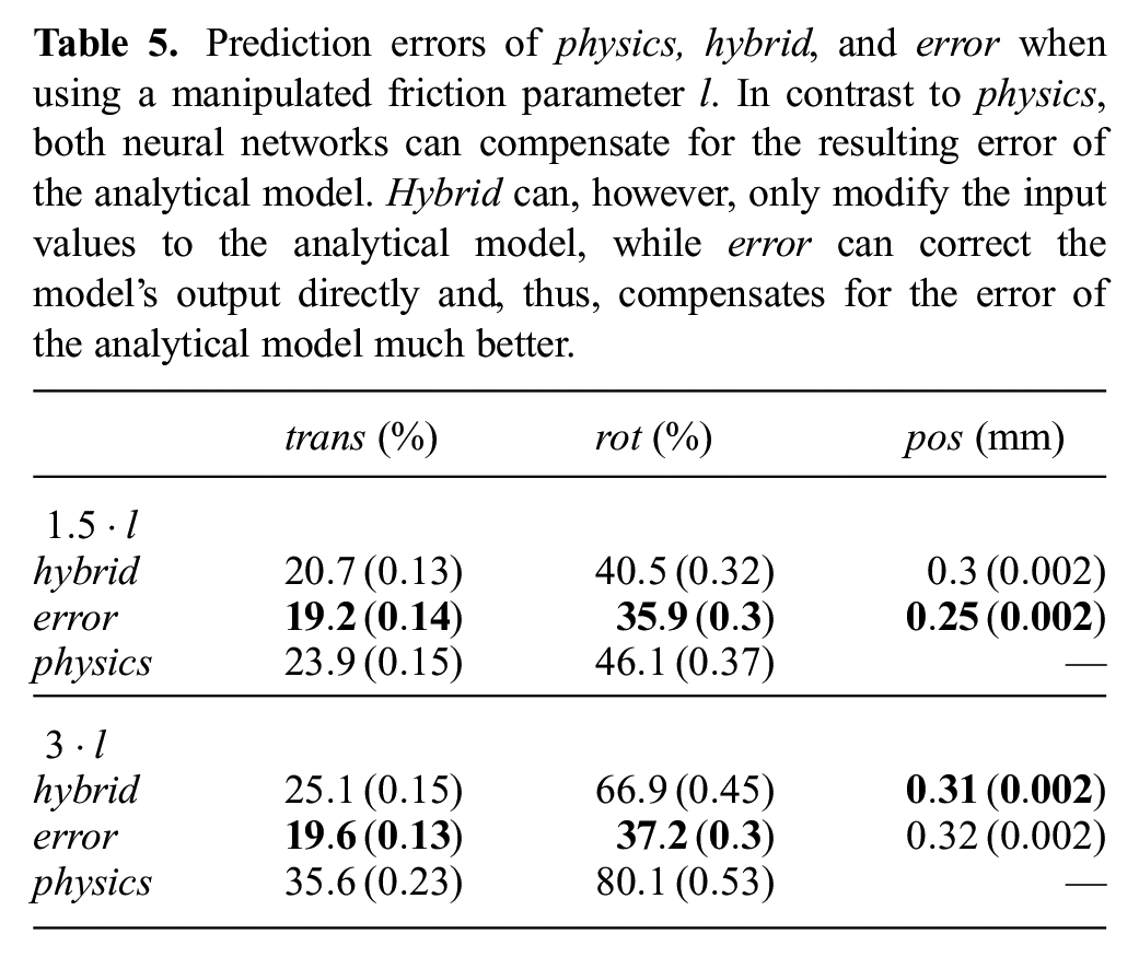
Wrong values of $l$ are especially harmful for predicting the rotation of the object, and both hybrid and error perform better than the physics baseline under this condition. This shows that the hybrid architecture has the ability to compensate for some errors of the analytical model by manipulating the predicted state representation. However, while hybrid performs similar to error if $l$ is only 1.5 times bigger than the correct value, it cannot compensate as well for larger deviations in $l$ . In this case, the ability of error to directly alter the output of the analytical model instead of only manipulating its input values proves to be necessary for achieving good performance.

The visualization in Figure 12 shows that both models predicted incorrect contact points to counter the effect of the higher friction value. This makes sense, since the location of the contact point influences the tradeoff between how much the object rotates and how much it translates. The predictions from error deviate farther from the ground truth values, which shows that the additional error-term does not prevent the model from manipulating the input values to the analytical model. Instead, it achieves its good results by combining both forms of correction.

Fig. 12.

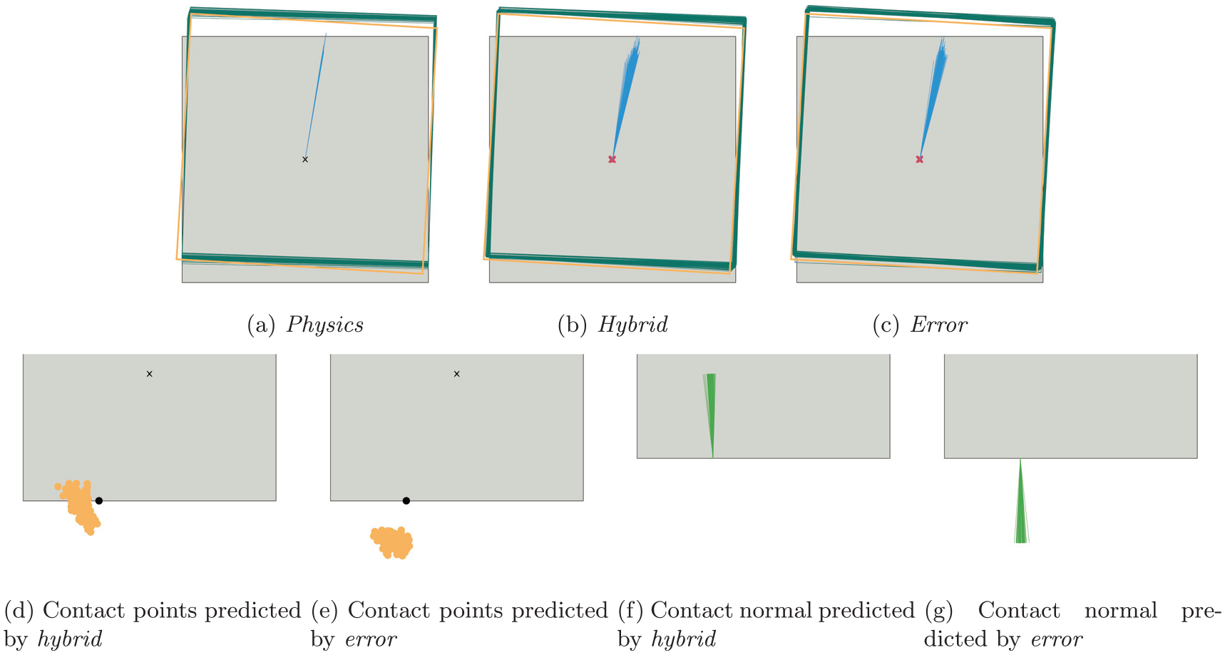
Predicted movement, contact points, and normals from 200 repeated pushes when using a wrong friction parameter ( $1.5·l$ ). The black point marks the (average) ground-truth contact point. Both networks compensate for the wrong friction parameter by predicting the contact point in a slightly wrong position, but the deviation from the ground truth is stronger for error, which also flips the direction of the predicted normal (this is, however, not relevant in our implementation of the analytical model).

5.8.3 Summary

Adding an learned error-correction term to the hybrid approach improves its ability to compensate for errors in the analytical model. It, however, does not prevent prediction of “wrong” state representations in such cases. For generalization, we found it helpful to limit the error term’s dependency on the magnitude of the pushing action and to stop gradient flow from the error to the perception module.

6 Extension to non-trivial viewpoints

In the previous section, we used depth images that showed a top-down view of the scene. This simplified the perception part and allowed us to focus our experiments on comparing the different architectures for learning the dynamics model. In this section, we briefly describe what changes when we move away from the top-down perspective and show that the proposed hybrid approach still works well on scenes that were recorded from an arbitrary viewpoint.

6.1 Challenges

For describing the scene geometrically, we need three coordinate frames, the world frame, the camera frame, and a frame that is attached to the object. In our rendered scenes, the origin of the world frame is located at the center of the table and its $x$ – $y$ plane is aligned with the table surface. The object frame is attached to the center of mass of the object. In planar pushing, we expect that the object only moves and rotates in the $x$ – $y$ plane of its supporting surface and the $x$ – $y$ plane of the object and world frame are thus aligned. The movement of the object is described relative to the world frame.

The camera frame is located at the sensor position and its $z$ -axis points towards the origin of the world frame. Depth images contain the distance of each visible point to the sensor along the $z$ -axis, i.e. the $z$ coordinates of said point in camera frame. Finally, a 3D point ${\left(\begin{array}{c}xyz\hfill \end{array}\right)}^{\mathrm{T}}$ in camera coordinates is mapped to a pixel ${\left(\begin{array}{c}uv\hfill \end{array}\right)}^{\mathrm{T}}$ by applying the perspective projection with focal length $f$ :

$$\left(\begin{array}{c}u\hfill \\ \multicolumn{1}{c}{v}\end{array}\right)=\frac{f}{z}\left(\begin{array}{c}x\hfill \\ \multicolumn{1}{c}{y}\end{array}\right)$$

(11)

In the special case of a top-down view, the $x$ – $y$ plane of world and camera frame are aligned, such that we can apply the analytical model presented in Section 3.1 in both frames. In addition, the measured depth ( $z$ in camera frame) of the table and the object are independent of their $x$ and $y$ position. This reduces the perspective projection to a scaling operation with a constant factor and allowed us to predict the object movement directly in pixel space. It also made segmenting the object very easy, since it is associated with one specific depth value.

Without the assumption of a top-down view, predicting object movement in pixel space becomes more challenging, since the same movement will span more pixels the further away the object is from the camera. In addition, perspective distortion now affects the shape and size of the objects in pixel space, which is, e.g., relevant for localizing the object.

6.2 Network architecture

We now describe the changes we made to the architectures from Section 5 to adapt to new camera configurations. To be able to relate pixel coordinates to 3D coordinates, we assume that we have access to the parameters of the camera (focal length) and the transform between camera and world frame.

6.2.1 Perception

The perception part remains mostly as it was before: we use the same architecture as shown in Figure 4. Inspired by Byravan and Fox (2017), we however extend the input data from depth images to full 3D point clouds. These point clouds are still image-shaped and can thus be treated as normal images whose channels encode coordinate values instead of colour or intensity.

As our architecture estimates the position of the object $\mathbf{o}$ in pixel space (using spatial softmax), we use the given camera parameters and transform to calculate the corresponding position in 3D world coordinates. For this, we need the $z$ coordinate (depth) of the predicted pixel location, which we obtain by interpolating between the values of the four pixels closest to the predicted coordinates. Owing to inaccuracies in the depth values and the projection matrix, this operation introduces an error of about 0.3 mm, which we however consider negligible.

6.2.2 Prediction and training

If we do not use a top-down view of the scene, the question becomes relevant in which coordinate frame the network should predict the contact point and the normal: pixel space, camera coordinates, or world coordinates. We decided to continue using pixel coordinates since predictions in this space can be most directly related to the input image and the predicted feature maps. To this end, we also transform the action into pixel space before using it (together with the glimpse encoding) as input for predicting the contact point and normal. Since the analytical model can only be used in the world frame where the movement of the object is limited to the $x$ – $y$ plane, we finally transform the predicted contact point and normal from pixel space to world coordinates. The resulting prediction part is illustrated in Figure 13. Note that the overall architecture (number and size of layers) is the same as for the top-down case (Figure 5).

Fig. 13.

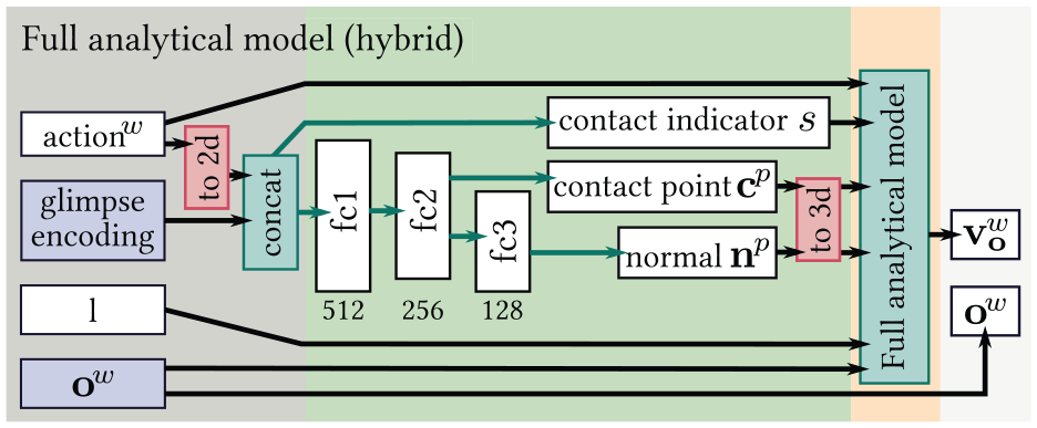
Prediction part of variant hybrid for non-trivial view points. While the analytical model operates in 3D world coordinates (indicated by ^w ), the contact point and normal are predicted in 2D pixel space (indicated by ^p ). Transforms from world coordinates to pixels and vice versa (red boxes) use the given depth values, camera parameters, and transform between camera and world frame. Please refer to Figure 5 for a detailed explanation of graphical elements.

We found training the model on data from arbitrary viewpoints more challenging than in the top-down scenario. To facilitate the process, we modified the network and the training loss to treat contact prediction and velocity prediction separately: instead of using the predicted contact indicator $s$ in the analytical model, the network now predicts $s$ as a separate output. We interpret $s$ as the probability that the pusher is in contact with the object and place a cross-entropy loss on it. For the predicted velocity, we only penalize errors if there was (ground-truth) contact. This prevents non-informative gradients to the velocity prediction if the object did not move and also solves the problem that the network tries to compensate for wrong velocity predictions by setting the contact estimate to zero.

At test time, the predicted contact indicator is multiplied with the predicted object movement from the analytical model to obtain the final velocity prediction.

The new loss for a single training example looks as follows: let $\hat{\mathit{s}}$ , ${\hat{\mathbf{v}}}_{\mathbf{o}}$ and $\hat{\mathbf{o}}$ denote the predicted and $\mathit{s}$ , ${\mathbf{v}}_o$ , $\mathbf{o}$ the real contact indicator, object movement, and position. Here $\mathbf{w}$ are the network weights and ${\nu }_{\mathbf{o}}=[v_{\mathrm{ox}},v_{\mathrm{oy}}]$ denotes linear object velocity:

$$\begin{array}{c}L(s,{\hat{\mathbf{v}}}_{\mathbf{o}},\hat{\mathbf{o}},\mathit{s},{\mathbf{v}}_o,\mathbf{o})=\mathrm{trans}+\mathrm{rot}+\mathrm{pos}+\cdots \hfill \\ +{\lambda }_1\mathrm{contact}+{\lambda }_2\sum _{\mathbf{w}}\Vert \mathbf{w}\Vert \hfill \\ \begin{array}{c}\mathrm{trans}=s\Vert {\hat{\nu }}_{\mathbf{o}}-{\nu }_{\mathbf{o}}\Vert \hfill \\ \multicolumn{1}{c}{\mathrm{rot}=s\frac{180}{\pi }|\omega -\hat{\omega }|}\\ \multicolumn{1}{c}{\mathrm{pos}=\Vert \mathbf{o}-\hat{\mathbf{o}}\Vert }\\ \multicolumn{1}{c}{\mathrm{contact}=-(s\log (\hat{s})+(1-s)\log (1-\hat{s}))}\end{array}\hfill \end{array}$$

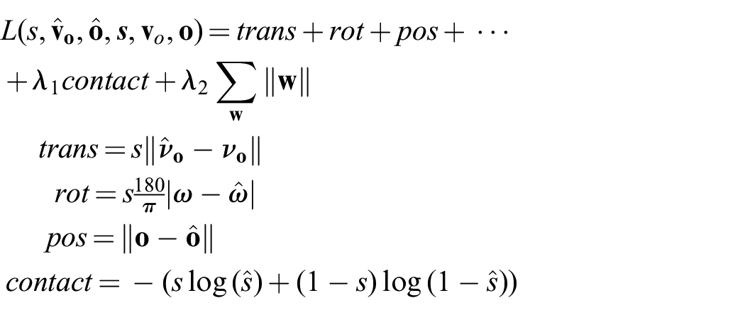
To ensure that all components of the loss are of the same magnitude, we compute translation and position error in millimeters and rotation in degrees. We set ${\lambda }_1=10$ and ${\lambda }_2=0.001$ .

6.3 Evaluation

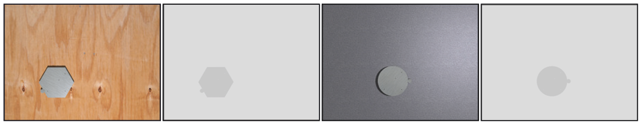
To show that our approach is not dependent on the top-down perspective, we train and evaluate it on images collected from a different viewpoint: the camera is located at $\left(\begin{array}{ccc}0\hfill & -0.25\hfill & 0.4\hfill \end{array}\right)$ in world coordinates, which corresponds to a more natural perspective where the viewer stands in front of the table instead of hovering above the table center. Figure 14 shows the depth channel of three examples.

Fig. 14.

Example depth images recorded from a non-top-down viewpoint. The depth values increase towards the back of the scene and the perspective transform affects the shape of the objects.

6.3.1 Data

As in Section 5, we use a dataset that contains all objects from the MIT Push dataset and all pushes with velocity $20$ mm/s for evaluating on this new viewpoint. We split it randomly into about 190,000 training examples and about 37,000 examples for testing.

6.3.2 Results

After 75,000 training steps, the hybrid model trained on the new viewpoint performs very similar to the one from the top-down case: $19.4\%$ translation error and $37.2\%$ error in rotation, as compared with $19.3\%$ and $36.1\%$ in the top-down case. The only notable difference is that the error in predicted position climbs from 0.32 to 1.12 mm. This can be partially explained by the inaccuracy introduced when converting from pixel coordinates to world coordinates. Another problem could be perspective distortion, as it influences shape and size of the objects depending on how close they are to the camera. In relation to the size of the object, an error of around 1 mm is, however, still very small.

6.3.3 Summary

The accuracy of our proposed method is not harmed by using a non-trivial camera viewpoint. We, however, require that the transform between world and camera coordinates as well as the camera parameters are known.

7 Conclusion and future work

In this article, we considered the problem of predicting the effect of physical interaction from raw sensory data. We compared a pure neural network approach with a hybrid approach that uses a neural network for perception and an analytical model for prediction. Our test bed involved pushing of planar objects on a surface: a nonlinear, discontinuous manipulation task for which we have both millions of data points and an analytical model.

We observed two main advantages of the hybrid architecture. Compared with the pure neural network, it significantly (i) reduces required training data and (ii) improves generalization to novel physical interaction. The analytical model aides generalization by limiting the ability of the hybrid architecture to overfit to the training data and by providing multiplication operations for scaling the output according to the input action and contact indicator. This kind of mathematical operation is hard to learn for fully connected architectures and requires many parameters and diverse training examples for covering a large value range. The drawback of the hybrid approach is that it cannot as easily improve on the performance of the underlying analytical model.

The pure neural network, on the other hand, can beat both the hybrid approach and the analytical model (with ground-truth input values) if trained on enough data. This, however, only holds when we evaluate on actions encountered during training and does not transfer to new push configurations, velocities, or object shapes. The challenge in these cases is that the distribution of the training and test data differ significantly.

To enable the hybrid approach to improve more on the prediction accuracy of its analytical model, we experimented with learning an error-correction term that is added to the prediction of the analytical model. These error models are almost as data efficient as hybrid and can to some extend retain the ability to generalize to different test data provided by the analytical model. However, they require more diversity in the training data than hybrid to avoid overfitting. Our experiments with a wrong analytical model also showed that the error models can compensate for errors of the model much better than hybrid, which can only influence the prediction by manipulating the input values of the analytical model.

The last architecture, simple, showed that combining learning and analytical models is not automatically guaranteed to lead to good performance. By replacing the first stage of the analytical model with a neural network, we instead combined the disadvantages of both approaches: the architecture needs lots of training data and does not generalize well to new pushes, because it misses the part of the analytical model that explains the influence of the pushing action on the resulting object velocity. In contrast to the pure neural network, however, it also cannot improve much on the performance of the analytical model.

A limitation of the presented hybrid approach is that it may be difficult to find an accurate analytical model for some physical processes and that not all existing models are suitable for our approach, as they e.g. need to be differentiable everywhere. In particular, the switching dynamics encountered when the contact situation changes proved to be challenging and more work needs to be done in this direction. If no analytical model is available, learning the predictive model with a neural network is still a very good option.

In perception on the other hand, the strengths of neural networks can be well exploited to extract the input parameters of the analytical model from raw sensory data. By training end-to-end through a given model, we can avoid the effort of labeling data with the ground-truth state. Our experiments also showed that training end-to-end allows the hybrid models to compensate for smaller errors in the analytical model by adjusting the predicted input values.

Using the state representation of the analytical model for the hybrid architecture has the advantage that the predictions of the network can be visualized and interpreted. This is not easy for the intermediate representations learned in the pure neural network. However, our results suggest that the pure neural network benefits from being free to chose its own state representation, as learning the dynamics model from the ground-truth state representation (neural dyn) lead to worse prediction results.

In the future, we want to extend our work to more complex perception problems, such as training on RGB images or scenes with multiple objects. An interesting question is whether perception on point clouds could be facilitated by using methods such as pointnet++ (Qi et al., 2017) that are specifically designed for this type of input data instead of treating the point cloud like a normal image.

A logical next step is also using our hybrid models for predicting more than one step into the future. Working on sequences makes it possible, for example, to guide learning by enforcing constraints such as temporal consistency or to exploit temporal cues such as optical flow. The model could also be used in a filtering scenario to track the state of an object and at the same time infer latent variables of the system such as the friction coefficients. Similarly, we can use the learned model to plan and execute robot actions using model predictive control.