Large-scale outdoor scene reconstruction and correction with vision

Abstract

We provide the theory and the system needed to create large-scale dense reconstructions for mobile-robotics applications: this stands in contrast to the object-centric reconstructions dominant in the literature. Our BOR²G system fuses data from multiple sensor modalities (cameras, lidars, or both) and regularizes the resulting 3D model. We use a compressed 3D data structure, which allows us to operate over a large scale. In addition, because of the paucity of surface observations by the camera and lidar sensors, we regularize over both two (camera depth maps) and three dimensions (voxel grid) to provide a local contextual prior for the reconstruction. Our regularizer reduces the median error between 27% and 36% in 7.3 km of dense reconstructions with a median accuracy between 4 and 8 cm. Our pipeline does not end with regularization. We take the unusual step to apply a learned correction mechanism that takes the global context of the reconstruction and adjusts the constructed mesh, addressing errors that are pathological to the first-pass camera-derived reconstruction. We evaluate our system using the Stanford Burghers of Calais, Imperial College ICL-NUIM, Oxford Broad Street (released with this paper), and the KITTI datasets. These latter datasets see us operating at a combined scale and accuracy not seen in the literature. We provide statistics for the metric errors in all surfaces created compared with those measured with 3D lidar as ground truth. We demonstrate our system in practice by reconstructing the inside of the EUROfusion Joint European Torus (JET) fusion reactor, located at the Culham Centre for Fusion Energy (UK Atomic Energy Authority) in Oxfordshire.

1. Introduction and previous work

This article is about the efficient generation of dense, colored models of very-large-scale environments from stereo cameras, laser data, or a combination thereof. Better maps make for better understanding; better understanding leads to better robots, but this comes at a cost. The computational and memory requirements of large dense models can be prohibitive.

Over the past few years, the development of 3D reconstruction systems has undergone an explosion facilitated by the advances in GPU hardware. Earlier, large-scale efforts such as those of Pollefeys et al. (2008), Agarwal et al. (2009), and Furukawa et al. (2010) reconstructed sections of urban scenes from unstructured photo collections. The ever-strengthening and broadening theoretical foundations of continuous optimization (Chambolle and Pock 2011; Goldluecke et al. 2012), upon which the most advanced algorithms rely, have become accessible for robotics and computer vision applications. Together these strands, hardware and theory, allow us to build systems that create large-scale 3D dense reconstructions as shown in Figure 2.

However, the state of the art of many dense 3D reconstruction systems rarely considers scalability for the practical use in mapping applications such as autonomous driving or inspection. The most general approaches are motivated by the recent mobile phone and tablet development (Klingensmith et al. 2015; Engel et al. 2015; Schöps et al. 2015) with an eye on small-scale reconstruction.

Several cultural heritage projects fuse multimodality sensor data to build high-fidelity representations of architectural and archeological sites with methods designed to support model capture using stationary lidar and motion photogrammetry (Moussa et al. 2012; Hess et al. 2015). In contrast to our system, these approaches involve manual intervention and editing at different stages of the pipeline to ensure the site is adequately captured.

Some researchers have worked with data and sensors more applicable for autonomous vehicles. Most notable, in 2010 Google released an academic article detailing their “Street View” application that utilizes laser and camera data to create dense 3D reconstructions of cities across the world (Anguelov et al. 2010). However, their algorithms over-emphasize the laser data and assume all depth maps only contain piecewise planar objects. In 2013, Google presented an alternative structure from motion approach using only camera sensors (Klingner et al. 2013). Xiao and Furukawa (2014) proposed a system to model large-scale indoor environments with laser and image inputs, but their modified Manhattan-world assumption restricted reconstructions from modeling anything other than vertical and horizontal planes. Bok et al. (2014) built upon the prior state of the art to create large-scale 3D maps using cameras and lasers. Their final reconstructions were sparse and only utilized the cameras for odometry and loop closure, not as an additional depth sensor to improve the dense reconstructions.

To this end, we propose a dense mapping system which meets the following requirements.

• R1: Operate in multiple-kilometer-scale environments.

• R2: No range limitations for input sensor observations.

• R3: Cope with a paucity of surface observations.

• R4: Fuse data from multiple sensor modalities.

These were designed to support our autonomous-driving applications. A survey of the literature found no systems currently exist which meet these requirements.

Four seminal systems (Table 1) in this area are dense tracking and mapping (DTAM) by Newcombe et al. (2011b), Kinect Fusion by Newcombe et al. (2011a), Kintinuous by Whelan et al. (2012), and voxel hashing by Nießner et al. (2013).

Table 1.

System capabilities comparison

Technique	R1: Env.	R2: Range	R3: Data	R4: Sensors
DTAM a	1 m2	1 m	100+ img/m2	Mono
Kinect Fusion	7 m2	2 m		RGB-D
Kintinuous	$\infty$	3 m		RGB-D
Voxel hashing	$\infty$	4 m		RGB-D
BOR2G b	$\infty$	50 m	0.05 img/m2	Mono, stereo or lidar

a

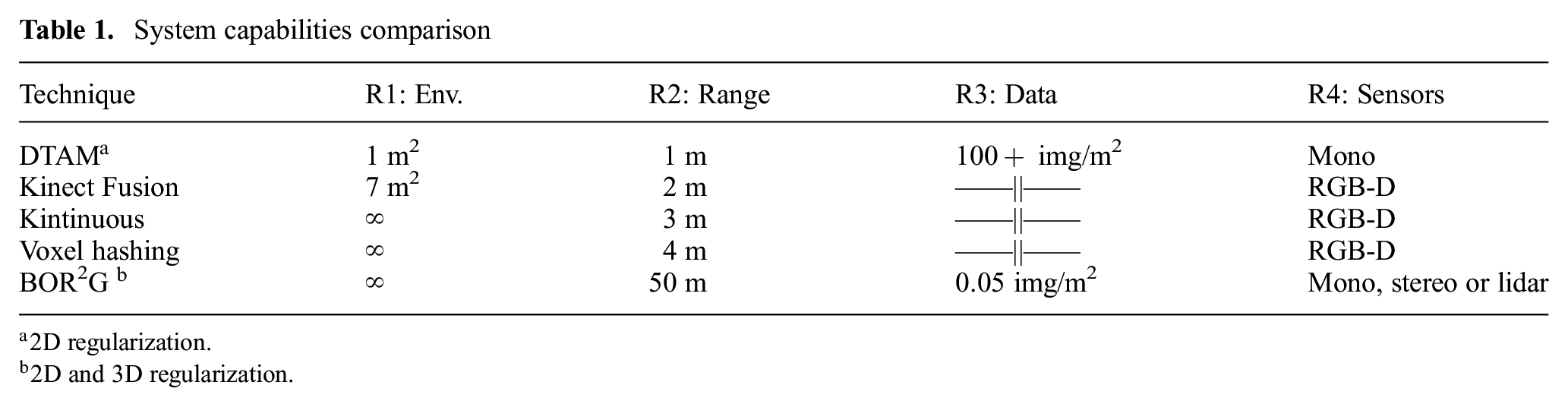
2D regularization.

b

2D and 3D regularization.

Before RGB-D cameras were widely available, DTAM presented a method to produce high-quality depth maps with a monocular camera. A cost volume is constructed in front of the camera’s focal plane and continually updated with 2D-regularized depth estimates from sequential image frames. The final reconstructions provide fine details, but this system limits the range of the monocular camera to near-field reconstructions.

In 2010, the first commodity RGB-D camera was released. RGB-D cameras provide a centimeter-level-accurate depth measurement for each pixel in the image: 640×480 resolution at 30 Hz in this first device. Curless and Levoy (1996) extended their work via the Kinect Fusion system to take advantage of this stream of high-frequency and high-quality depth maps. Leveraging the truncated signed distance function (TSDF), depth observations are stored in a voxel grid where each voxel contains a positive number when in front of a surface and a negative number behind the surface. Solving for the zero-value level set results in a dense model of the original surface. Thus, Kinect Fusion could generate unprecedented-quality dense 3D reconstructions in real time for workspaces approximately 7 m³ in size.

In contrast to Kinect Fusion where the voxel grid is fixed to one location in space, Kintinuous sought to extend the size of reconstruction scenes by allowing the voxel grid to move with the camera. A continual stream of previously observed regions are streamed to disk as a mesh, but can be reloaded back into the GPU if that region is observed again. This system theoretically infinitely extended the reconstruction workspace size. However, it cannot leverage sensor observations further than 3 m from the RGB-D camera because it is still fundamentally based upon a conventional fixed-size voxel grid.

Nießner’s hashing voxel grids (HVG) also extended the size of reconstructions but did so instead by only allocating voxels in regions where surfaces were observed. This removed memory wasted storing free space. When combined with streaming of data to/from the GPU and hard disk when surfaces are “far” away from the sensor, there is essentially no limit on the size of reconstructions. This implementation restricts the sensor range to 4 m as that is near the maximum effective range of the Kinect camera, however the range can be trivially extended. Solutions such as that of Whelan et al. (2014) leverage a rolling cyclical buffer as the volumetric-reconstruction data structure. This is an interesting approach that allows local volumetric regions to virtually translate as the camera moves through an environment. The correct choice of an efficient volumetric data structure has also gained attention in the deep learning context where it affects the resolution of 3D tasks, including 3D object classification, orientation estimation, and point-cloud labeling (Riegler et al. 2017)

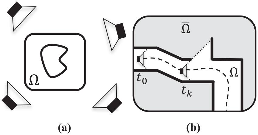
Most of the previously described techniques focused on object-centered reconstructions. In other words, the operator selected a small scene to reconstruct (e.g., desk, courtyard, etc.) and a single sensor was moved through the environment in a way that observed all surfaces multiple times from a variety of angles. This results in a fine-detailed final reconstruction, as shown in Figure 1(a). In autonomous driving scenarios where the sensor is mounted on a vehicle and the path is not known a priori, the surfaces are observed fewer times. In fact, we found that RGB-D scenarios have over 3,100 times more depth images per square meter than our autonomous vehicle applications (Table 2).

Fig. 1.

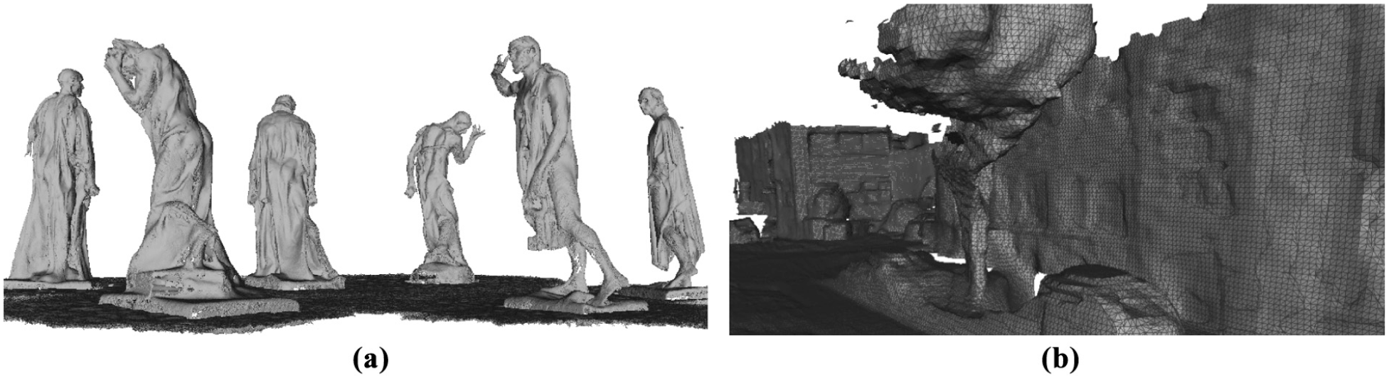
RGB-D versus KITTI reconstruction detail comparison. (a) Stanford Burghers of Calais: 155.97 depth images/m². (b) KITTI-VO 00: 0.049 stereo images/m². Both reconstructions were created with the BOR²G pipeline, but the Stanford reconstruction (Zhou and Koltun 2013) has over 3,100 times (Table 2) more depth observations per square meter than the KITTI reconstruction. In addition, each of the RGB-D depth maps are more than an order of magnitude more accurate than the stereo-camera-generated depth estimates. This article is focused on creating high-quality reconstructions that gracefully handle KITTI-level low observation densities over kilometers of observations, but also works on the traditional RGB-D use-cases. In addition, our method accepts sensor input from RGB-D, stereo images, lidar, or a combination thereof. When compared with the model provided by Zhou and Koltun (2013), the above BOR²G Burghers reconstruction has a median point-to-surface difference of 0.5 cm. Section 7 provides a more detailed quantitative analysis our reconstruction precision.

Table 2.

Summary of reconstruction scenarios

Dataset	Cam. Dist.	# Frames	Surface	Frames/m2
KITTI-VO 00	3.8 km	4,541	93,546 m2	0.049
KITTI-VO 05	2.2 km	2,761	55,909 m2	0.049
KITTI-VO 06	1.2 km	1,101	23,585 m2	0.047
Burghers	0.2 km	11,230	72 m2	155.97

In addition, mobile-robotics sensor suites typically include lidars and forward-facing monocular or stereo cameras. Since the viewing range of RGB-D cameras is so short (5 m) and their accuracy degrades outdoors, they are not useful when reconstructing an urban environment from a mobile-robotics platform. Cameras on mobile-robotics platforms produce significantly less-accurate depth measurements. Over time, lidar sensors usually have a smaller reconstruction field of view and depth-observation density than a similarly placed camera sensor. Both camera and lidar sensors observe surfaces far fewer times than in a typical RGB-D scenario. Therefore, the reconstructions inherently have less detail, as shown in Figure 1(b), which requires us to apply contextual priors via a local regularizer to improve the final surface reconstructions.

Tables 1 and 2 and Figure 1 summarize the preceding literature review.

Our contributions in this article are as follows.

1. We present in Sections 2–6 the theory required to construct a state-of-the-art dense-reconstruction pipeline for mobile-robotics applications (i.e., satisfies R1–R4 defined in this section). Our implementation includes a compressed data structure (R1/R2) of a sensor-agnostic voxel grid (R4). Since the input data may be noisy and the observations per square meter are very low, we utilize a regularizer in two and three dimensions to both serve as a prior and reduce the noise in the final reconstruction (R3).

2. We present in Sections 5.3–5.4 a method to regularize 3D data stored in a compressed volumetric data structure thereby enabling optimal regularization of significantly larger scenes (fulfills R1 and R3). The key difficulty (and, hence, our vital contribution) in regularizing within a compressed structure is the presence of many additional boundary conditions introduced between regions which have and have not been directly observed by the range sensor. Accurately computing the gradient and divergence operators, both of which are required to minimize the regularizer’s energy, becomes a non-trivial problem. We ensure the regularizer only operates on meaningful data and does not extrapolate into unobserved regions.

3. We present in Section 6 a method to adjust reconstructions and correct gross errors with priors learned from high-fidelity historical data (e.g., roads generally do not have holes in them, cars are of certain shapes, etc.) We show that appearance and geometry features can be extracted from a 3D reconstruction, and better depth maps can be produced with a neural network that applies these priors. We illustrate how this step can be included in our dense-reconstruction pipeline to produce more comprehensive meshes.

4. We provide, by way of our quantitative results in Section 7 and the models released in the supplementary materials, a new KITTI benchmark for the community to compare dense reconstructions. In addition, we include the ground-truth (GT) data used to evaluate our system. This includes the optimized vehicle trajectory, consolidated GT pointcloud, and final dense reconstructions with different sensor modalities.

5. We release (Section 7.3) the 1.6 km Oxford Broad Street dataset (partial example reconstruction in Figure 2) as a real-world reconstruction scenario for a mobile-robotics platform with a variety of camera and lidar sensors.

Fig. 2.

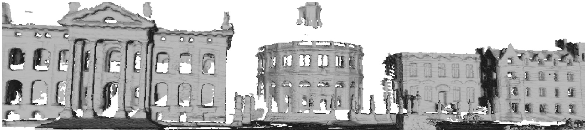
This article is about the efficient generation of dense models of multiple-kilometer-scale environments from stereo and/or laser data. This is an example reconstruction from the 1.6 km Oxford Broad Street dataset released with this article.

Our hope is that our dataset and benchmarks become valuable tools for comparisons within the community.

This article builds upon our prior work (Tanner et al. 2015, 2018) by enabling regularization in a compressed 3D data structure; evaluating the relative reconstruction quality based on using combinations of camera and laser sensors; documenting the performance of signed distance function (SDF) and histogram data terms for the regularizer; correcting reconstructions using historical priors; and using a full simultaneous localization and mapping (SLAM) approach to evaluate the improved reconstruction quality when revisiting a location.

2. System overview

This section provides a brief overview of our system architecture (Figure 3) before we proceed to a detailed discussion in Sections 3–6.

Fig. 3.

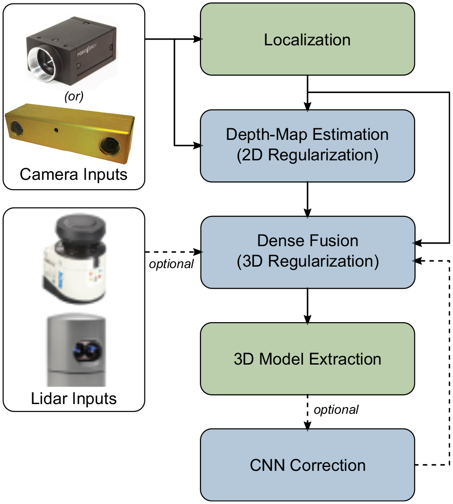
An overview of our software pipeline. Our dense fusion module accepts data from either laser sensors or depth maps created from mono or stereo cameras. We regularize the 3D model, extract the surface, and apply learned corrections to the meshes. Then, we provide the final 3D model to other components on our autonomous robotics platform, e.g., segmentation, localization, planning, or visualization. The blue modules are discussed in further detail in Sections 3–6.

At its core, our system consumes a stream of stereo camera images (I) or laser scans (L) and produces a 3D model. The pipeline consists of a localization module, which provides sensor pose estimates. We place no requirements on the trajectory of the source sensors; indeed, we illustrate our method using images captured from a forward-facing camera on a road vehicle, an ill-conditioned use-case that is challenging yet likely given the utility of forward-facing cameras in navigation and perception tasks. The design of this module is versatile allowing us to pick any arbitrary SLAM derivative; we choose ORB-SLAM2 (Mur-Artal and Tardós 2015) as it is a widely used, open-source benchmark tool for localization and loop closure with monocular, stereo, and RGB-D cameras.

The depth-map estimation module (Section 4) processes a stream of stereo or monocular frames into a stream of 2D regularized depth maps, D. Owing to the nature of a passive camera and the large scale at which we operate, we utilize a sophisticated regularizer, specifically, the total generalized variation (TGV) regularizer, to improve the accuracy of these depth maps.

The dense fusion module (Section 5) merges the regularized depth maps into a compressed data structure as a SDF, $f:{\mathrm{\Omega }}_3\to \mathbb{R}$ , where ${\mathrm{\Omega }}_3\subset {\mathbb{R}}^3$ represents a subset of points in 3D space. New incoming data can be added at any time from any suitable sensor source. Even with the regularized input depth maps, the resulting reconstruction tends to contain spurious and noisy surfaces. Our 3D total variation (TV) regularizer operates over ${\mathrm{\Omega }}_3$ to generate the optimized, denoised SDF field, $u:{\mathrm{\Omega }}_3\to \mathbb{R}$ . This regularizer also serves as a prior to aid in the reconstruction even with a paucity of direct surface observations (Figure 1).

The convolutional neural network (CNN) correction step (Section 6) further improves reconstructions created from low-quality or scarce data. Our approach corrects the 3D geometry based on prior knowledge of how certain scenarios are expected to look when reconstructed. We achieve this by projecting various features in training 3D reconstructions into 2D images and using a CNN to learn the differences between high- and low-quality data. Learned error correction, along with regularization in both two and three dimensions are the salient features of our system.

A final surface model is extracted to be processed in parallel by a separate application (e.g., segmentation, localization, planning, or visualization).

3. Optimization with TV

In this article, we address the inverse problem of estimating the 3D dense structure of an environment given a set of 2D images and/or 3D sparse laser scans. Inverse problems deal with the estimation of unknown quantities u (structure in our case) given their effects f (images or laser data). By their nature, these problems are ill-posed, which means that at least one of the following three requirements is not met: existence of a solution, uniqueness of the solution, or stability of the solution (i.e., small changes in input data produce small changes in the result). Clearly the problem we try to solve is ill-posed. As an extreme example, if we want to reconstruct a white wall from a set of images, we cannot guarantee uniqueness and stability (walls at different distances and orientations will produce the same observations).

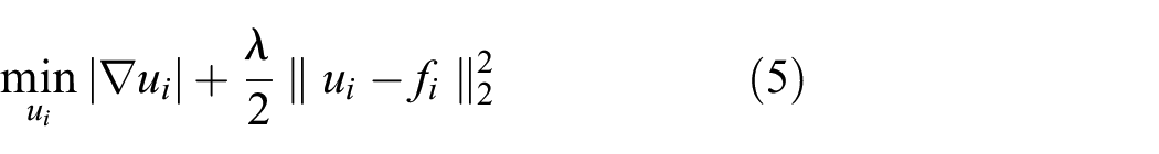
The properties of the problem can improve if we limit the space of meaningful solutions by imposing regularity assumptions or prior knowledge about the solution. Energy-based minimization approaches model these requirements by using an energy regularization term that favors certain solutions and a data term that models how well the searched solution u explains the set of observations f. The following equation synthesizes this approach,

$$\underset{u}{\min }{E}_{\mathrm{reg}}(u)+E_{\mathrm{data}}(f,u)$$

(1)

where $E_{\mathrm{reg}}(u)$ is the regularization or “smoothness” term and $E_{\mathrm{data}}(f,u)$ is the data-fidelity term.

In this article, we use a first-order ( $\alpha =1$ ) and a second-order ( $\alpha =2$ ) TGV^α regularization term, respectively, in the optimizations performed in the depth-map estimation and the 3D dense fusion blocks in Figure 3. As we discuss later, these regularizers allow us to incorporate prior information about the type of surfaces we expect to encounter in the traversed environment.

Let us now present a simple denoising problem that will help us to illustrate the primal–dual algorithm (Chambolle and Pock 2011) implemented to solve Equation (1) in the following sections. For simplicity, we employ a first-order TGV¹ regularizer also known as TV. Figure 4(left) shows the effect of the TV on a noisy 1D signal $f(t)$ defined in the bounded domain ${\mathrm{\Omega }}_1=[t_0,t_n]$ , where ${\mathrm{\Omega }}_1\subset \mathbb{R}$ . The energy to be minimized is given by

$$E(u)={\int }_{{\mathrm{\Omega }}_1}|\nabla u|d{\mathrm{\Omega }}_1+\frac{\lambda }{2}{\int }_{{\mathrm{\Omega }}_1}\parallel u-f{\parallel }_2^{2}d{\mathrm{\Omega }}_1$$

(2)

where ${\int }_{{\mathrm{\Omega }}_1}|\nabla u|d{\mathrm{\Omega }}_1$ is the TV of the solution and, in this case, we use a quadratic penalty for the data term. Note that the TV accumulates the magnitude of local variations in the signal and therefore measures its total length. Intuitively, the TV term tends to reduce signal ripples and therefore filters out high-frequency noise while maintaining big discontinuities present in the data term. In the extreme case when no data term is available, TV would produce a constant solution $u=\mathrm{const}.$ since then $\nabla u=0$ . On the other hand, the data term tries to preserve the shape of the input data $f(t)$ . The trade off between both terms is controlled by $\lambda$ , which, when tuned correctly, favors piece-wise constant solutions. To solve this problem we first discretize Equation (2),

$$E(u)=\sum _{i=0}^{n-1}|\nabla u_i|+\frac{\lambda }{2}\sum _{i=0}^n\parallel u_i-f_i{\parallel }_2^2$$

(3)

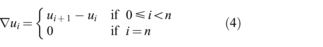
where we calculate the gradient using forward differences and we assume zero Neumann boundary conditions: the value of the gradient at the borders is $0$ , i.e., we assume the signal remains constant outside the left and right boundaries,

$$\nabla u_i=\{\begin{array}{cc}{u}_{i+1}-u_i\hfill & \mathrm{if}0\le i<n\hfill \\ \multicolumn{1}{c}{0}& \mathrm{if}i=n\hfill \end{array}$$

(4)

Fig. 4.

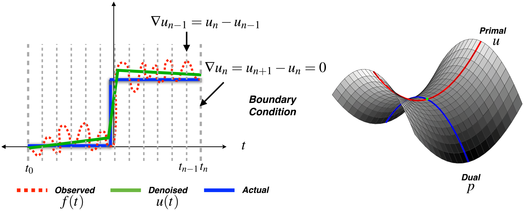
(Left) Example of a denoised 1D signal with TV. The aim of the continuous energy minimization is to recover a function $u(t)$ given the observed signal $f(t)$ defined in the continuous domain ${\mathrm{\Omega }}_1=[t_0,t_n]$ . TV regularization filters out high-frequency noise preserving sharp discontinuities. We impose zero Neumann boundary conditions that assume the signal remains constant outside the left and right boundaries. (Right) The original non-differentiable energy minimization is transformed into a smooth primal–dual problem by applying the Legendre–Fenchel transform to the TV term. The resulting saddle point problem can be solved by alternating variants of gradient descent and gradient ascent steps for the primal u and dual p variables, respectively.

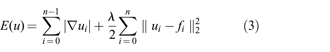
To simplify the explanation let us minimize Equation (3) with respect to the ith sample in the summation,

$$\underset{u_i}{min}|\nabla u_i|+\frac{\lambda }{2}\parallel u_i-f_i{\parallel }_2^2$$

(5)

Although this problem is convex and, therefore, its global minimum can be computed, standard optimization algorithms such as gradient descent or Newton and quasi-Newton methods cannot be applied directly because they require smooth cost functions to assure convergence (Nocedal and Wright 2006). In this case, the gradient is not defined at the kink of the absolute value. The Legendre–Fenchel transform (Rockafellar 1970) provides an elegant way to convert the $L_1$ norm into a maximization problem that, although more complex, is differentiable (see Figure 5 for an intuitive explanation),

$$|\nabla u_i|=\underset{|p_i|\le 1}{sup}〈\nabla u_i,p_i〉$$

(6)

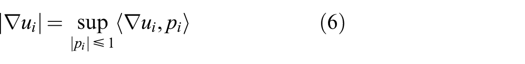
where the operator 〈•,•〉 computes the inner product of its operands and $p_i$ is known as the dual variable, which represents for each $u_i$ the sub-gradient of the $L_1$ norm. Substituting Equation (6) into Equation (5), we obtain

$$\underset{u_i}{min}\underset{|p_i|\le 1}{sup}〈\nabla u_i,p_i〉+\frac{\lambda }{2}\parallel u_i-f_i{\parallel }_2^2$$

(7)

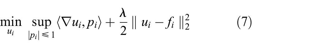
which is a saddle point problem with equivalent primal and dual solutions since strong duality holds (Boyd and Vandenberghe 2004). Figure 4(right) shows an example of a saddle point problem in u and p with zero duality gap.

Fig. 5.

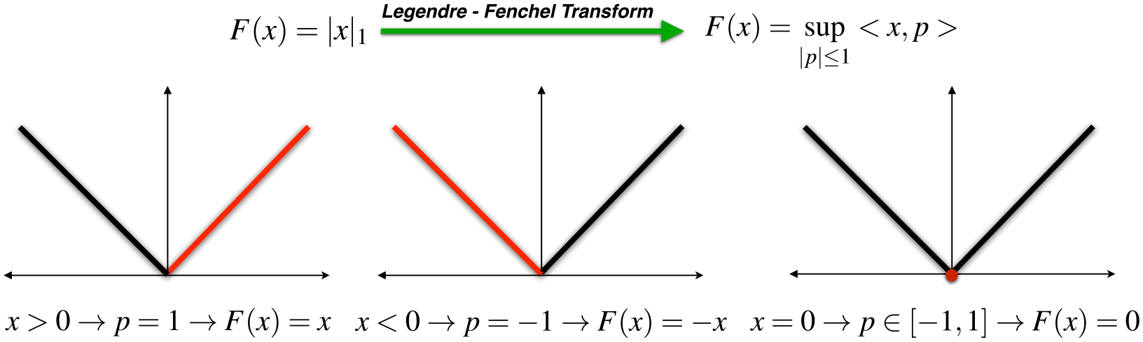
Legendre–Fenchel transform of the non-differentiable $L_1$ norm. In the 1D case, the norm is represented by the absolute value $|x{|}_1$ , which is a non-smooth function whose gradient is not determined at $x=0$ . A more convenient representation, that allows us to apply well-known optimization techniques, consists of transforming the original function into a maximization problem with linear inequality constraints. To show that both the original and the transformed representation are equivalent, we can demonstrate that the solution of the maximization problem leads indeed to the original $L_1$ norm: when $x>0$ (left), the value of p that maximizes the expression subject to the constraint $|p|\le 1$ is $p=1$ , therefore $F(x)=x=|x|$ ; when (center), the inner product is maximized when $p=-1$ leading to $F(x)=-x=|x|$ . Finally, when $x=0$ , any value of p in the feasible set $[-1,1]$ gives the same solution $F(x)=0$ . Note that, as a result of applying the Legendre–Fenchel transform, we have transformed a simple but non-differentiable expression $|x{|}_1$ into a more complex but smooth problem for which we can apply well-known optimization algorithms such as projected gradient ascent.

An equivalent energy expression, that will be useful in the derivation of the optimization algorithm, can be obtained by calculating the adjoint $\mathrm{Adj}(•)$ of the linear operator ∇. When $\nabla u$ , and therefore $\mathbf{p}$ , is n-dimensional (with $n>1$ ), the adjoint of the gradient is equal to the negative of the divergence operator: $\mathrm{Adj}(\nabla )\mathbf{p}=-\nabla ·\mathbf{p}=-({\nabla }_1{p}^1+\dots +{\nabla }_n{p}^n)$ where ${\nabla }_j{p}^j$ is the $j^{\mathrm{th}}$ directional derivative of the last component of $\mathbf{p}$ , we will use as well $(\nabla ·\mathbf{p}{)}^j={\nabla }_j{p}^j$ . By definition a linear operator and its adjoint fulfill,

$$〈\nabla u_i,{\mathbf{p}}_i〉=-〈u_i,\nabla ·{\mathbf{p}}_i〉$$

(8)

To satisfy this equation, forward differences and Neumann boundary conditions for the gradient become backward differences and Dirichlet boundary conditions for the divergence, the value of the variable at the borders is $0$ ,

$$(\nabla ·{\mathbf{p}}_i{)}^j=\{\begin{array}{cc}{p}_i^j-p_{i-1}^j\hfill & \mathrm{if}0<i<n\hfill \\ \multicolumn{1}{c}{p_i^j}& \mathrm{if}i=0\hfill \\ \multicolumn{1}{c}{-p_{i-1}^j}& \mathrm{if}i=n\hfill \end{array}$$

(9)

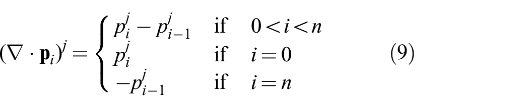
With a little abuse of notation, we use the divergence operator for the current 1D example (j can only be equal to 1). Using the adjoint of the gradient we can rewrite Equation (7) as

$$\underset{u_i}{min}\underset{|p_i|\le 1}{sup}-〈u_i,\nabla ·p_i〉+\frac{\lambda }{2}\parallel u_i-f_i{\parallel }_2^2$$

(10)

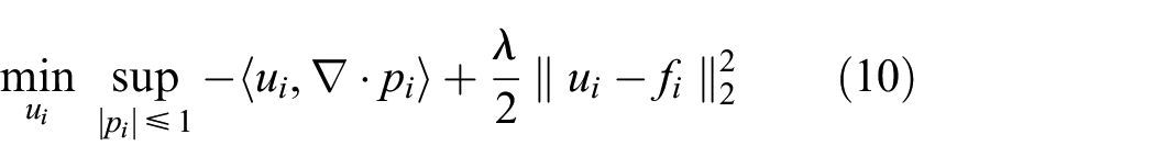
The primal–dual optimization algorithm (Chambolle and Pock 2011) to solve Equation (7) or its equivalent Equation (10) consists of the following steps.

1. Initialize $p_i$ , $u_i$ , and ${\hat{u}}_i$ to $0$ . Here ${\hat{u}}_i$ is a temporary variable which reduces the number of optimization iterations required to converge.

2. To solve the maximization we use a projected gradient ascent algorithm. The gradient of Equation (7) with respect to $p_i$ is just $\nabla {\hat{u}}_i$ (as we explained previously, we use ${\hat{u}}_i$ instead of $u_i$ to speed up the convergence of the algorithm, more details are provided by Chambolle and Pock (2011)). Therefore, $p_i^{\mathrm{new}}=p_i+\sigma \nabla {\hat{u}}_i$ where $\sigma$ is the dual variable’s gradient-ascent step size. Since $p_i^{\mathrm{new}}\in [-1,1]$ we project the solution into the feasible set using a projection operator $\pi (p_i^{\mathrm{new}})$ . Therefore, the maximization step is given by

   $$\begin{array}{c}{p}_i=\pi (p_i+{\sigma }_p\nabla {\hat{u}}_i)\hfill \\ \pi (p_i)=\frac{p_i}{max(1,|p_i|)}\hfill \end{array}$$

   (11)

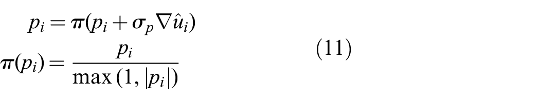
3. The minimization is based on a look-ahead gradient descent algorithm. In this case, it is easier to calculate the gradient with respect to $u_i$ from Equation (10). With look-ahead, we mean that the gradient is not evaluated at the current solution but at the new estimate $u_i^{\mathrm{new}}$ after the step is taken. Deriving Equation (10) with respect to $u_i$ and evaluating at $u_i^{\mathrm{new}}$ the gradient is given by $-\nabla ·p_i+\lambda (u_i^{\mathrm{new}}-f_i)$ . Applying a gradient descent step with step size $\tau$ , we obtain

   $$u_i^{\mathrm{new}}=u_i-\tau (-\nabla ·p_i+\lambda (u_i^{\mathrm{new}}-f_i))$$

   (12)

   which gives an implicit equation in $u_i^{\mathrm{new}}$ . Rearranging terms, the primal step is

   $$u_i^{\mathrm{new}}=\frac{u_i+\tau \nabla ·p_i+\tau \lambda f_i}{1+\tau \lambda }$$

   (13)

4. To reduce the number of required iterations we apply the following “relaxation” step,

   $${\hat{u}}_i=u_i+\theta (u_i-{\hat{u}}_i)$$

   (14)

   where $\theta$ is a parameter to adjust the relaxation step size.

   Finally, we repeat steps 2–4 until convergence.

In the following two sections, we make use of the primal–dual algorithm to regularize both a stream of 2D depth maps (Section 4) and the final 3D dense reconstruction (Section 5).

4. Depth-map estimation

Given a pair of rectified images captured from a stereo camera, we implement an algorithm based on Ranftl et al. (2012) that allows us to calculate very high-quality disparity maps. Although many other dense stereo approaches exist in the literature (a nice survey is presented by Scharstein and Szeliski 2002), most of the solutions require explicit strategies to handle occlusions. Instead, we implement an energy minimization approach with an $L_1$ -fidelity data term that provides some robustness against outliers from occlusions while handling varying illumination and radiometric differences between the cameras. For regularization we use a second-order regularizer term that favors piecewise planar disparity maps and allows sub-pixel accurate solutions. The energy to be minimized is

$$E(d)=E_{\mathrm{reg}}(d)+E_{\mathrm{data}}(d;I_L,I_R)$$

(15)

where d is the searched disparity image defined in ${\mathrm{\Omega }}_2\subset {\mathbb{R}}^2$ .

4.1. Data term

To improve robustness against outliers we implement an $L_1$ -norm penalty term that penalizes photo-consistency differences between matched pixels in the images,

$$E_{\mathrm{data}}(d;I_L,I_R)={\int }_{{\mathrm{\Omega }}_2}|\nabla C_W(I_L(x+d,y),I_R(x,y))|d{\mathrm{\Omega }}_2$$

(16)

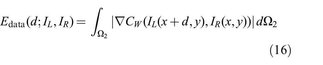
In particular, $\nabla C_W(•)$ denotes the difference between the census transform signature (CTS) (Zabih andWoodfill 1994) of two pixels calculated in a window of size W for a candidate disparity d. This metric has been shown to be both illumination invariant and fast to compute in comparison to other metrics such as the sum of absolute distances (SAD), the sum of square distances (SSD) or the normalized cross correlation (NCC) (Zabih and Woodfill 1994). Its computation is simple: given a pixel, the CTS computes a bit string by comparing the chosen pixel with the local window W centered around it. A bit is set to 1 if the corresponding pixel has a lower intensity than the pixel of interest. The difference between two windows $\nabla C_W(•)$ is then given by the Hamming distance between the two bit strings defining them.

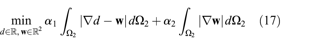
4.2. Affine regularization

As we explained in the previous section, for ill-posed problems, such as depth-map estimation, good and apt priors are essential, whether the prior is task-specific and bespoke (Güney and Geiger 2015) or more general. A common choice is to use TV regularization as a prior to favor piecewise-constant solutions. However, its use lends itself to poor depth-map estimates over outdoor sequences because it assumes fronto-parallel surfaces. Figure 6 shows some of the artifacts created after back-projecting the point cloud for planar surfaces not orthogonal to the image plane (e.g., the roads and walls that dominate our urban scenes). Thus, we reach for a second-order total generalized variation (TGV²) regularization term (Bredies et al. 2010), which favors affine surfaces,

$$\underset{d\in \mathbb{R},\mathbf{w}\in {\mathbb{R}}^2}{min}{\alpha }_1{\int }_{{\mathrm{\Omega }}_2}|\nabla d-\mathbf{w}|d{\mathrm{\Omega }}_2+{\alpha }_2{\int }_{{\mathrm{\Omega }}_2}|\nabla \mathbf{w}|d{\mathrm{\Omega }}_2$$

(17)

where $\mathbf{w}$ allows the disparity d in a region of the depth map to change at a constant rate and therefore creates planar surfaces with different orientations. Here ${\alpha }_1$ and ${\alpha }_2$ are free parameters (Table 3).

Fig. 6.

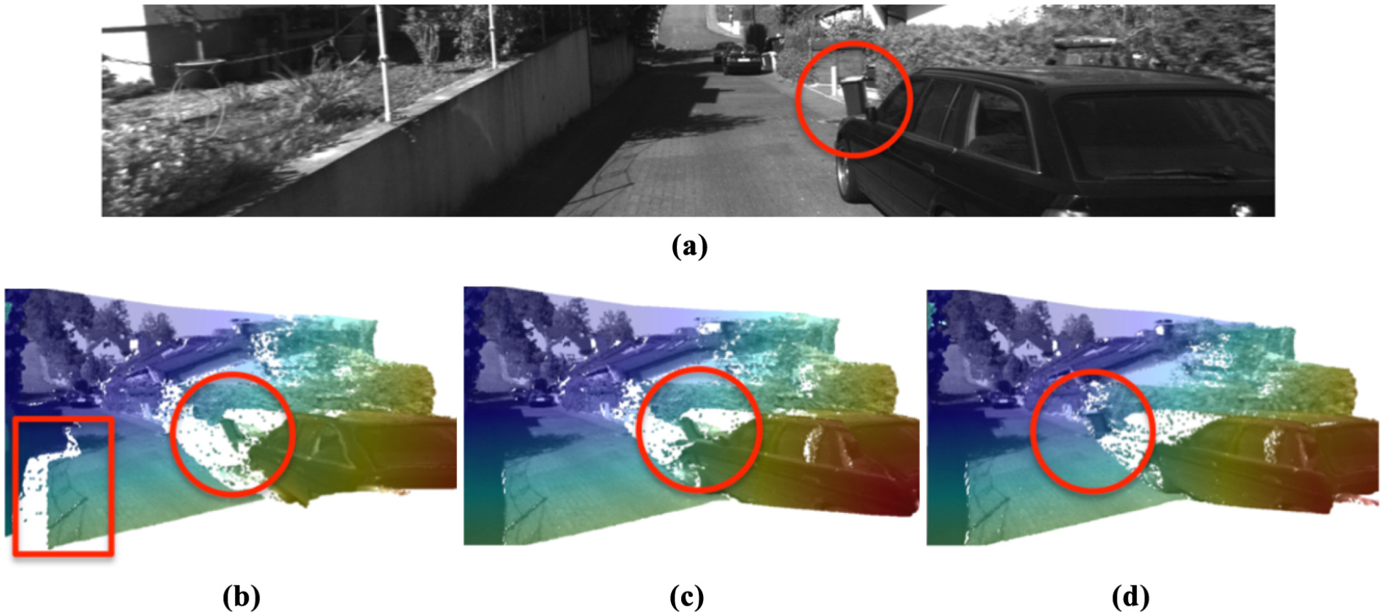
Comparison of three 2D depth-map regularizers: TV, TGV, and TGV-Tensor. Using the reference image (a), the TV regularizer (b) favors fronto-parallel surfaces, therefore it creates a sharp discontinuity for the shadow on the road (red rectangle) and attaches the rubbish bin to the front of the car (red circle). TGV (c) improves upon this by allowing planes at any orientation, but it still cannot identify boundaries between objects: the rubbish bin is again estimated as part of the car. Finally, the TGV-Tensor (d) regularizer both allows planes at any orientation and is more successful at differentiating objects by taking into account the normal of the gradient of the color image. For clarity, the sparse reconstructions have a different viewing origin than the reference image.

Table 3.

Summary of parameters used in the system

Symbol	Value	Description
${\lambda }_{3D}$	0.8 (10 cm)/0.4 (20 cm)	The TV weighting of the data term versus regularization
${\mu }_{3D}$	1.0 m (10 cm)/1.6 m (20 cm)	The maximum voxel distance behind a surface in which to fuse negativesigned-distance values
${\sigma }_p$ , $\theta$	0.5, 1.0	3D regularizer gradient-ascent/descent step sizes
$\tau$	$1/6$	3D regularizer relaxation-step weight
N	20	Number of histogram bins
${\lambda }_{2D}$	0.5	The TGV weighting of the data term versus regularization
${\alpha }_1,{\alpha }_2$	1.0, 5.0	Relative weights of the affine-smooth/piecewise-constant TGV terms
$\beta$ , $\gamma$	1.0, 4.0	Exponent and scale factor, respectively, modifying the influence of the image gradient

To minimize this problem using the primal–dual algorithm explained in the previous section, we apply the Legendre–Fenchel transform to both summands in Equation (17) so that both terms become differentiable,

$$\begin{array}{c}|\nabla d-\mathbf{w}|=\underset{|\mathbf{p}{|}_{\infty }\le 1}{sup}〈\nabla d-\mathbf{w},\mathbf{p}〈\hfill \\ |\nabla \mathbf{w}|=\underset{|\mathbf{q}{|}_{\infty }\le 1}{sup}〈\nabla \mathbf{w},\mathbf{q}〈\hfill \end{array}$$

(18)

Note that, this time, two additional dual variables $\mathbf{p}\in {\mathbb{R}}^2$ and $\mathbf{q}\in {\mathbb{R}}^4$ are added to the optimization.

4.3. Leveraging appearance

A common problem that arises during the energy minimization is the resulting tension between preserving object discontinuities while respecting the smoothness prior. Ideally the solutions preserve intra-object continuity and inter-object discontinuity. For example, in Figure 6 we desire to accurately estimate the depths of both the rubbish bin and automobile (intra-object consistency), but we also must account for their position relative to one another (inter-object discontinuity).

One may mitigate this tension by using an inhomogeneous diffusion coefficient $c(|\nabla I|)$ in the energy as an indicator of boundaries between objects,

$$\underset{d\in \mathbb{R},\mathbf{w}\in {\mathbb{R}}^2}{min}{\alpha }_1{\int }_{{\mathrm{\Omega }}_2}|c(|\nabla I|)\nabla d-\mathbf{w}|d{\mathrm{\Omega }}_2+{\alpha }_2{\int }_{{\mathrm{\Omega }}_2}|\nabla \mathbf{w}|d{\mathrm{\Omega }}_2$$

(19)

where $c(|\nabla I|)$ is defined as

$$c(|\nabla I|)=\exp (-\gamma |\nabla I{|}^{\beta })$$

(20)

However, though this aids the regularizer, it does not contain information about the direction of the border between the objects. To take this information into account we adopt an anisotropic diffusion tensor,

$$\underset{d\in \mathbb{R},\mathbf{w}\in {\mathbb{R}}^2}{min}{\alpha }_1{\int }_{{\mathrm{\Omega }}_2}|\mathbf{T}\nabla d-\mathbf{w}|d{\mathrm{\Omega }}_2+{\alpha }_2{\int }_{{\mathrm{\Omega }}_2}|\nabla \mathbf{w}|d{\mathrm{\Omega }}_2$$

(21)

with

$$\mathbf{T}=\exp (-\gamma |\nabla I{|}^{\beta })n{n}^T+n^{\perp }{n}^{{\perp }^T}$$

(22)

where $n=\frac{\nabla I}{|\nabla I|}$ and $n^{\perp }$ is its orthogonal complement. Here $\gamma$ and $\beta$ are free parameters (Table 3). The effect of this tensor on Equation (22) is to decompose the components of the disparity gradient $\nabla d$ in directions aligned with the gradient of the image n and orthogonal to it $n^{\perp }$ . We do not smooth depth discontinuities aligned with n but we penalize large image gradient components aligned with $n^{\perp }$ . In other words, if there is a discontinuity visible in the color image, then it is highly probable that there is a discontinuity in the depth image. The benefits of this tensor term are visually depicted in Figure 6.

5. Dense 3D fusion

The core of the 3D dense mapping system consists of a dense fusion module that integrates a sequence of depth/range observations (depth maps from Section 4 or laser scans) into a volumetric representation. To smooth noisy surfaces and remove uncertain surfaces, our system carries out an energy optimization on the data volume together with 3D regularization.

5.1. Fusing data

Our aim is to efficiently reconstruct urban outdoor environments while continually improving the accuracy of the representation with subsequent observations. Our data fusion system is built to process depth-map estimates (camera sensor) and range observations (lidar sensor) within the same data structure. The representation of the surfaces plays an important role in our system. An explicit representation of each of the depth/range observations (e.g., as a point cloud) is a poor choice as storage grows without bound and the surface reconstruction does not improve when revisiting a location.

Instead, we prefer an implicit representation of the surface. A common approach is to select a subset of space in which one will reconstruct surfaces and divide that subspace into a uniform voxel grid. Each voxel stores depth/range observations represented by their corresponding TSDF, $u_{\mathrm{TSDF}}$ (Curless and Levoy 1996). The TSDF value of each voxel is computed such that one can globally solve for the zero-crossing level set (isosurface) to find a continuous surface model. Even though the voxel grid is a discrete field, because the TSDF value stores the precise distance to the nearest surface, the surface reconstruction is even more precise than the voxel size.

Owing to memory constraints, only a small subset of space (a few cubic meters) can be reconstructed using a conventional approach where the voxel grid is fixed in space (Newcombe et al. 2011a,b). This presents a particular problem in mobile-robotics applications since the exploration region of the robot would be restricted to a prohibitively small region. In addition, long-range depth/range sensors (e.g., laser, stereo-camera-based depth maps) cannot be fully utilized since their range exceeds the size of the voxel grid (or local voxel grid if a local-mapping approach is used) (Whelan et al. 2012), as shown in Table 1.

In recent years, a variety of techniques have been proposed to remove these limits (Whelan et al. 2012; Nießner et al. 2013; Chen et al. 2013). They leverage the fact that the overwhelming majority of voxels do not contain any valid TSDF data since they are never directly observed by the range sensor. A compressed data structure only allocates and stores data in voxels that are near a surface.

One of the more prolific compression approaches is Nießner et al.’s (2013) HVG. HVG creates an “infinite” (within numerical limitation) virtual grid that subdivides the environment with a coarse and fine level of detail (see Figure 7). The coarse level contains voxel blocks (small conventional voxel grids composed of $8\times 8\times 8$ voxels) while the fine level contains voxels. No memory is used on the GPU until a surface is observed within that voxel block ( $\pm \mu$ ).

Fig. 7.

A depiction of our novel combination of the HVG data structure with regularization to optimally fuse depth observations from the environment: (a) physical-space representation; (b) GPU-memory representation. The HVG enables us to reconstruct large-scale scenes by only allocating memory for the regions of space in which surfaces are observed (i.e., the colored blocks). A location in the physical operating environment is mapped to a bucket index in GPU memory (gray circle number) via a hash function. The bucket may be thought of as a linked list to deconflict hash collisions. To avoid generating spurious surfaces, we mark each voxel with an indicator variable ( $1_{{\mathrm{\Omega }}_3}$ ) to ensure the regularizer only operates on voxels in which depth information was observed directly. This same approach is used independent of the range sensor, e.g., stereo depth maps or lasers. The rationale behind ${\mathrm{\Omega }}_3$ and ${\overline{\mathrm{\Omega }}}_3$ is described in Section 5.3. Figure inspired by Nießner et al. (2013).

As part of initialization, the HVG algorithm reserves a portion of the GPU memory to store $n_{\mathrm{blocks}}$ of voxel blocks. In addition, and as part of the overhead, a hash table with $n_{\mathrm{hash}}$ elements (where $n_{\mathrm{hash}}>>n_{\mathrm{blocks}}$ ) enables efficient lookup and reservation of voxel blocks during run time. Applying a hash function to coordinates in world space deterministically computes the index within the hash table, which in turn points to the $8\times 8\times 8$ voxel grid of SDF data. We refer the reader to the original HVG paper (Nießner et al. 2013) for further implementation details.

Fusing data into the voxel grid varies depending on whether we are using a camera-based sensor (Section 5.1.1) or a laser-based sensor (Section 5.1.2).

5.1.1. Depth-map fusion

Unlike conventional voxel grids, HVG requires a two-step data-fusion process because voxel blocks in which data is fused may not yet be reserved in the hash table. The voxel blocks are reserved first by efficiently ray casting (Amanatides et al. 1987) the depth map and reserving memory from the range $d\pm \mu$ .

Once memory is reserved, the data fusion is similar between conventional voxel grids and HVG. If one considers each HVG voxel block to be a conventional voxel grid, then the update equations are nearly identical to those presented by Newcombe et al. (2011a). For each voxel allocated in memory, perform the following operations on every new depth map, D.

1. Calculate the voxel’s global-frame center ${\mathbf{p}}_g=[x_g,y_g,z_g{]}^{\mathrm{T}}$ with respect to the camera coordinate frame as ${\mathbf{p}}_c={\mathbf{T}}_{\mathrm{gc}}^{-1}{\mathbf{p}}_g$ , where ${\mathbf{T}}_{\mathrm{gc}}\in \mathbb{S}\mathbb{E}(3)$ is the camera-to-global coordinate frame transformation.

2. Project ${\mathbf{p}}_c$ into D to determine the nearest pixel $d_{x,y}$ .

3. If the pixel $(x,y)$ lies within the depth map, evaluate $u_{\mathrm{SDF}}=d_{x,y}-z_c$ . Here $u_{\mathrm{SDF}}>0$ indicates the voxel is between the surface and the camera, $u_{\mathrm{SDF}}<0$ indicates voxels are occluded from the camera by the surface, and $u_{\mathrm{SDF}}=0$ indicates voxel centroids that exactly intersect the surface.

4. Update the voxel’s current f (SDF value) and w (weight or confidence in f) at time k,

   $$\begin{array}{c}{w}_k=\{\begin{array}{cc}{w}_{k-1}+1\hfill & u_{\mathrm{SDF}}\ge -\mu \hfill \\ \multicolumn{1}{c}{w_{k-1}}& u_{\mathrm{SDF}}<-\mu \hfill \end{array}\hfill \\ \multicolumn{1}{c}{f_k=\{\begin{array}{cc}\frac{u_{\mathrm{SDF}}+w_{k-1}{f}_{k-1}}{w_k}\hfill & u_{\mathrm{SDF}}\ge -\mu \hfill \\ \multicolumn{1}{c}{f_{k-1}}& u_{\mathrm{SDF}}<-\mu \hfill \end{array}}\end{array}$$

   (23)

   where $w_{k-1}$ and $f_{k-1}$ are the previous values of f and w for that voxel.

Note, we initially elected to use the SDF rather than the TSDF for f as this allows us to simultaneously fuse data from different sensors, each with distinct $\mu$ values based on the sensor’s precision, into the same voxel grid. For example, $\mu$ might be large for points far away from the stereo camera but be smaller for laser scans or close stereo observations. However, in practice, we found a fixed $\mu$ value based on the sensor accuracy (Table 3) produced better results. When using multiple sensor modalities, we selected $\mu$ based on the least accurate sensor.

This fusion process is well suited for real-time processing on a GPU (via CUDA or OpenCL) as, once the memory is properly allocated, no atomic operations are required to fuse a depth map into the voxel grid. Each voxel can be allocated an individual GPU thread to compute the updated f and w values.

5.1.2. Laser fusion

Fusing laser data into the voxel grid is accomplished via an efficient ray-casting implementation (Amanatides et al. 1987). Consider the case of a single laser ray ( $\overrightarrow{\mathbf{\rho }}$ ) with an origin at ${\mathbf{\rho }}_o$ and a termination (i.e., where the laser struck a surface) point at ${\mathbf{\rho }}_t$ . Here $\overrightarrow{\mathbf{\rho }}$ is fused into the voxel grid by tracing the ray and updating each voxel with the signed distance to ${\mathbf{\rho }}_t$ . Specifically, the following operations are performed on all voxels which intersect the ray from ${\mathbf{\rho }}_o$ to ${\mathbf{\rho }}_t$ .

1. Calculate the voxel’s global-frame center ${\mathbf{p}}_g=[x_g,y_g,z_g{]}^{\mathrm{T}}$ .

2. Compute the vector from the origin of the laser scan to the current voxel center: ${\mathit{v}}_1={\mathbf{p}}_g-{\mathbf{\rho }}_o$ .

3. Compute the vector from the current voxel center to the termination point of the laser scan: ${\mathit{v}}_2={\mathbf{\rho }}_t-{\mathbf{p}}_g$ .

4. Compute the voxel’s SDF value:

   $u_{\mathrm{SDF}}=\mathrm{sgn}({\mathit{v}}_1·{\mathit{v}}_2)\parallel {\mathit{v}}_2{\parallel }_2$

   If $u_{\mathrm{SDF}}>0$ , the voxel is between the surface and the laser sensor, $u_{\mathrm{SDF}}<0$ indicates the surface occludes the laser sensor’s view of the voxel, and $u_{\mathrm{SDF}}=0$ indicates the voxel’s centroid exactly intersects the surface.

5. Update the voxel’s current f (SDF value) and w (weight) via Equation (23).

As with the depth-map fusion, these calculations are highly data-independent and, thus, suitable for parallel processing. However, in contrast to depth-map fusion, one must ensure the memory update operations are atomic since multiple laser rays may simultaneously intersect any given voxel.

To conserve space, voxel blocks are allocated in memory for the region $\pm \mu$ , but voxels between the sensor and observed surface are updated (if they exist). This removes free-space violations without increasing the memory requirements. In other words, in addition to the memory allocated to store the observed surface, we ray trace between the surface and the sensor to update any voxel blocks that may have previously been allocated when fusing depth or range data. For example, if an automobile appeared in a previous depth map but it has since moved, the full ray trace will update the SDF values in those now-empty voxels (i.e., “delete” the now-spurious automobile reconstruction).

5.2. Energy for 3D reconstruction

Both inputs to our system pipeline, stereo-image-based depth maps and laser scans, are noisy, especially when compared with the centimeter-level accuracy of RGB-D systems. As explained in Section 3, we pose the noise-reduction problem as a continuous energy minimization

$$E(u)=E_{\mathrm{reg}}(u)+E_{\mathrm{data}}(u,f)$$

(24)

where f represents noisy SDF data and u is the optimally denoised SDF, both of which are defined in the 3D domain ${\mathrm{\Omega }}_3\subset {\mathbb{R}}^3$ .

For the regularization term, we first implemented a second-order 3D TGV² regularizer (TGV² provided the high-quality 2D depth-map results in Section 4), but we found that the simpler first-order TV regularizer produces nearly identical results. We believe this is because the size of the voxels is very small relative to the size of the surfaces being reconstructed. The frontal-parallel and piece-wise discontinuity effects are therefore minimal, so we selected the 3D TV regularizer as it has significantly lower computational and memory requirements while producing similar results. In practice, the TV norm has a two-fold effect: (1) smooths out the reconstructed surfaces; and (2) removes surfaces that are “uncertain,” i.e., voxels with high gradients and few direct observations. This includes removing surfaces with very small surface area, but also serves to smooth out larger surfaces.

We propose two implementations for the data term: the first method (Section 5.2.1) averages all depth measurements, whereas the second method (Section 5.2.2) records the depth measurements as samples from a probability-density function (PDF) in a histogram data structure.

5.2.1. SDF data term

In the method originally proposed by Curless and Levoy (1996) and popularized by Newcombe et al. (2011a), data is fused into the voxel grid by storing in each voxel a weighted average of all depth observations. To produce good results, this method usually requires the noise to either be small or Gaussian.

The end result of fusion (Equation (23)) are two numbers stored in each voxel: (1) f, the signed metric distance to the nearest surface; and (2) w, the number of observations used to compute f. One may also think of f and w as storing the mean (f) and information (w, inverse of variance) to characterize the sampled distribution. As the energy minimization seeks to solve for a denoised version of f, a simple $L_2$ norm data term ensures the final u is consistent with the observed depths:

$$E(u)={\int }_{{\mathrm{\Omega }}_3}|\nabla u{|}_{1}d{\mathrm{\Omega }}_3+\frac{\lambda }{2}{\int }_{{\mathrm{\Omega }}_3}\parallel f-u{\parallel }_2^{2}d{\mathrm{\Omega }}_3$$

(25)

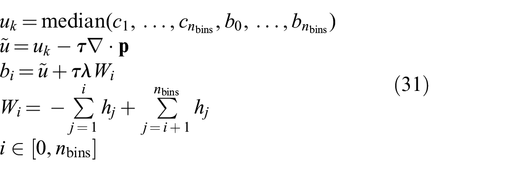
5.2.2 Histogram data term

In general, the more meaningful information provided to an optimizer, the better the final results. The SDF data-term method summarized all depth measurements for a voxel as two numbers: f and w. At the other extreme, one could store the entire set of N observed SDFs within each voxel (Zach et al. 2007),

$$E(u)={\int }_{{\mathrm{\Omega }}_3}|\nabla u|d{\mathrm{\Omega }}_3+\frac{\lambda }{2}{\int }_{{\mathrm{\Omega }}_3}\frac{1}{N}\sum _{t=1}^N\parallel f_t-u{\parallel }_{1}d{\mathrm{\Omega }}_3$$

(26)

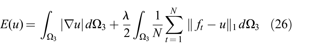
The main drawback with this approach is that we cannot just sequentially update a single f and w when a new depth map arrives. Instead, all previous $u_{\mathrm{SDF}}$ values must be stored in each voxel. This greatly limits the number of depth maps that can be fused due to memory constraints.

A more practical approach is to store depth measurements as a histogram representing the PDF for that voxel rather than explicitly storing the entire history of observations or the mean and variance (Zach 2008). This histogram approach is desirable since it uses a fixed amount of memory.

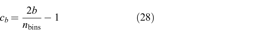
With a histogram representation, each voxel contains an array with $n_{\mathrm{bins}}$ elements where each element, $h_b$ , stores the number of depth observations within the bth histogram bin. The fusion process described in the previous section is thus augmented by linear scale-and-clamp f in the interval $[-1,1)$ . The relationship between SDF, TSDF, and histogram bins is graphically depicted in Figure 8.

Fig. 8.

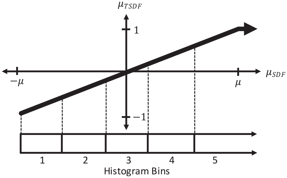
Visual depiction of the relationship between the TSDF, SDF, and histogram bins storage methods for voxel distance values. TSDF has traditionally been the favored approach, but SDF is useful when fusing multiple sensor modalities so that each sensor has a different $\mu$ based on its precision. The histogram approach is useful to aid the regularizer by directly storing a PDF (versus the weighted average stored by SDF/TSDF) of noisy surface measurements.

The energy minimization becomes

$$E(u)={\int }_{{\mathrm{\Omega }}_3}|\nabla u|d{\mathrm{\Omega }}_3+\frac{\lambda }{2}{\int }_{{\mathrm{\Omega }}_3}\sum _{b=1}^{n_{\mathrm{bins}}}{h}_b\parallel c_b-u{\parallel }_{1}d{\mathrm{\Omega }}_3$$

(27)

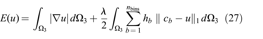
where the center of the bins are computed as

$$c_b=\frac{2b}{n_{\mathrm{bins}}}-1$$

(28)

This method has been demonstrated by Zach (2008) on a small-scale, object-centered environment where the final reconstruction was within a millimeter of the GT laser scan with 99% completeness.

5.3. Omega Domain

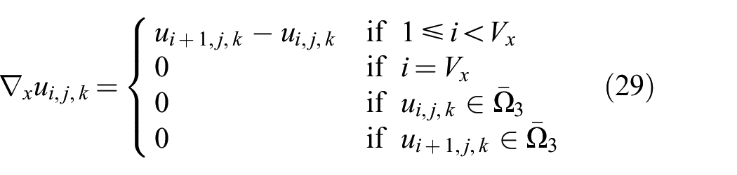
Since we are moving at an a priori unknown trajectory through the world, we only observe surfaces in a subset of all allocated voxels and voxel blocks. We therefore present a new technique to prevent the unobserved voxels from negatively affecting the regularization results of the observed voxels, i.e., to ensure the regularizer does not extrapolate into unobserved regions. To achieve this, as illustrated in Figure 9, we define the complete voxel grid domain as $\Lambda$ and use ${\mathrm{\Omega }}_3$ to represent the subset of voxels that have been observed directly and that will be regularized. The remaining subset, ${\overline{\mathrm{\Omega }}}_3$ , represents voxels which have never been observed. By definition, ${\mathrm{\Omega }}_3$ and ${\overline{\mathrm{\Omega }}}_3$ form a partition of $\Lambda$ and therefore $\Lambda ={\mathrm{\Omega }}_3\cup {\overline{\mathrm{\Omega }}}_3$ and ${\mathrm{\Omega }}_3\cap {\overline{\mathrm{\Omega }}}_3=\mathrm{Ø}$ .

Fig. 9.

Traditional voxel-grid-based reconstructions focus on object-centred applications where the objects are fully observed multiple times from various angles: (a) object-centered fusion; (b) mobile-robot-centered fusion. Even though the internal portion of the object has not been observed, previous regularization techniques do not make a distinction between ${\mathrm{\Omega }}_3$ (observed regions) and ${\overline{\mathrm{\Omega }}}_3$ (unobserved regions). However, in mobile-robotics applications the world environment is traversed and observed during exploration, requiring voxels that were never observed directly. For example, at camera capture $t_x$ , it is unknown what exists in the camera’s upper field of view. Not accounting for ${\overline{\mathrm{\Omega }}}_3$ in regularization results in incorrect surface generation.

To the best of the authors’ knowledge, all prior works rely on a fully observed conventional voxel grid before regularization and they implicitly assume that $\Lambda ={\mathrm{\Omega }}_3$ , i.e., every voxel in the voxel grid is observed directly by the sensor. In our mobile-robotics platform, this assumption is not valid. The robot motion results in unobserved regions caused by object occlusion, field-of-view limitations, and trajectory decisions. Therefore, ${\mathrm{\Omega }}_3\subset \Lambda$ as Figure 9 illustrates.

Our approach introduces a new state variable, $1_{{\mathrm{\Omega }}_3}:\Lambda \to \{0,1\}$ , in each voxel indicating whether it was directly observed by a range sensor. Therefore, ${\mathrm{\Omega }}_3$ is the set solely upon which the regularizer is constrained to operate. In our previous work, we found that failure to account for these boundary conditions creates spurious surfaces in non-valid voxels ( ${\overline{\mathrm{\Omega }}}_3$ ) (Tanner et al. 2015; Tanner et al. 2016). Note that all voxel blocks that are not allocated are in ${\overline{\mathrm{\Omega }}}_3$ . A graphical depiction of how we augmented the HVG data structure with ${\mathrm{\Omega }}_3$ and ${\overline{\mathrm{\Omega }}}_3$ is provided in Figure 7.

Since compressed voxel grid data structures are not regular in space, the proper method to compute the gradient (and its dual: divergence) in the presence of the additional boundary conditions (caused by the ${\mathrm{\Omega }}_3$ domain and voxel-block boundaries) is not straightforward. We define the gradient as

$${\nabla }_x{u}_{i,j,k}=\{\begin{array}{cc}{u}_{i+1,j,k}-u_{i,j,k}\hfill & \mathrm{if}1\le i<V_x\hfill \\ \multicolumn{1}{c}{0}& \mathrm{if}i=V_x\hfill \\ \multicolumn{1}{c}{0}& \mathrm{if}{u}_{i,j,k}\in {\overline{\mathrm{\Omega }}}_3\hfill \\ \multicolumn{1}{c}{0}& \mathrm{if}{u}_{i+1,j,k}\in {\overline{\mathrm{\Omega }}}_3\hfill \end{array}$$

(29)

where $u_{i,j,k}$ is a voxel’s TSDF value at the 3D world integer coordinates $(i,j,k)$ , and $V_x$ is the number of voxels in the x dimension. The gradient term in the regularizer encourages smoothness across neighboring voxels, which explains why this new gradient definition excludes ${\overline{\mathrm{\Omega }}}_3$ voxels: they have not been observed.

To solve the primal–dual optimization (Section 3), we also need to define the corresponding divergence operator:

$$(\nabla ·{\mathbf{p}}_{i,j,k}{)}^x=\{\begin{array}{cc}{\mathbf{p}}_{i,j,k}^x-{\mathbf{p}}_{i-1,j,k}^x\hfill & \mathrm{if}1<i<V_x\hfill \\ \multicolumn{1}{c}{{\mathbf{p}}_{i,j,k}^x}& \mathrm{if}i=1\hfill \\ \multicolumn{1}{c}{-{\mathbf{p}}_{i-1,j,k}^x}& \mathrm{if}i=V_x\hfill \\ \multicolumn{1}{c}{0}& \mathrm{if}{u}_{i,j,k}\in {\overline{\mathrm{\Omega }}}_3\hfill \\ \multicolumn{1}{c}{{\mathbf{p}}_{i,j,k}^x}& \mathrm{if}{u}_{i-1,j,k}\in {\overline{\mathrm{\Omega }}}_3\hfill \\ \multicolumn{1}{c}{-{\mathbf{p}}_{i-1,j,k}^x}& \mathrm{if}{u}_{i+1,j,k}\in {\overline{\mathrm{\Omega }}}_3\hfill \end{array}$$

(30)

Each voxel block is treated as a voxel grid with boundary conditions that are determined by its neighbors’ ${\mathrm{\Omega }}_3$ indicator function, $1_{{\mathrm{\Omega }}_3}$ . The regularizer operates only on the voxels within ${\mathrm{\Omega }}_3$ , the domain of integration, and thus it neither spreads spurious surfaces into unobserved regions nor updates valid voxels with invalid SDF data.

Note that both equations are presented for the x dimension, but the y and z dimension equations can be obtained by variable substitution between i, j, and k.

5.4. 3D energy minimization

In the following two subsections, we describe the algorithm to solve Equations (25) and (27). We point the reader to Rockafellar (1970), Chambolle and Pock (2011), Handa et al. (2011), and Piniés et al. (2015) for a detailed derivation of these steps. We vary from their methods in our new definition for the gradient and divergence operators, as described in Section 5.3.

5.4.1. SDF optimization implementation

The optimization described in Equation (25) is a 3D version of the primal–dual TV algorithm explained in Section 3. We just need to use the new definitions of the gradient and the divergence operator defined previously.

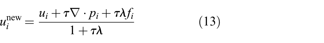
5.4.2. Histogram optimization implementation

Again, the implementation to minimize the histogram-based approach closely mirrors the implementation described Section 3. The only difference is that the primal update (Equation (13)) becomes

$$\begin{array}{c}{u}_k=\mathrm{median}(c_1,\dots ,c_{n_{\mathrm{bins}}},b_0,\dots ,b_{n_{\mathrm{bins}}})\hfill \\ \multicolumn{1}{c}{\tilde{u}=u_k-\tau \nabla ·\mathbf{p}}\\ \multicolumn{1}{c}{b_i=\tilde{u}+\tau \lambda W_i}\\ \multicolumn{1}{c}{W_i=-\sum _{j=1}^i{h}_j+\sum _{j=i+1}^{n_{\mathrm{bins}}}{h}_j}\\ \multicolumn{1}{c}{i\in [0,n_{\mathrm{bins}}]}\end{array}$$

(31)

where $u_k$ is the primal solution at the kth optimization iteration, and $W_i$ and $b_i$ are the optimal weight and gradient-ascent solution for the ith histogram bin.

For both the SDF and histogram optimization implementations, the operations in each voxel are independent. Therefore, our implementations leverage massively parallel GPU processing with careful synchronization between subsequent primal and dual variable updates.

5.5. Data structures

To summarize the key data tracked during the data fusion and 3D regularization stages our pipeline, we define the following three voxel datatypes:

Listing 1: Voxel data structures

struct VoxelSdf {

 float sdf;

 uint8_t weight;

 uint8_t color[3];

 bool is_omega;

};

struct VoxelHistogram {

 uint8_t histogram[N_BINS];

 uint8_t color[3];

 bool is_omega;

};

struct VoxelTotalVariation {

 float u; // primal

 float p[3]; // dual

 float u_relax; // relaxation step

};

Sensor data (stereo-camera-based depth maps or laser) is continually fused into either VoxelSdf or VoxelHistogram voxel grid. In practice, we found the laser data works best with VoxelSdf and the camera-based depth maps work well (in the tested scenarios) with either VoxelSdf or VoxelHistogram. Section 7 provides a more detailed analysis on why this is the case.

Depth-map fusion color is read directly from the RGB reference image. When fusing lidar scans, the color is the grayscale reflectance intensity value. If both lidar and depth images are fused into the same voxel grid, color data always takes priority over grayscale data to make the final model visually appealing (i.e., surfaces viewed by the camera are colored correctly while surfaces viewed only by the laser are grayscale).

Once all data is fused, the energy minimization data is stored in a voxel grid of type VoxelTotalVariation. The final surface may be extracted directly from the VoxelTotalVariation voxel grid via marching cubes (Lorensen and Cline 1987) or ray casting (Amanatides et al. 1987) to solve for the zero-crossing level set of u.

6. Learned corrections and prior application

The final step in our pipeline is a system that uses prior knowledge of scene appearance and geometry to detect and correct missing data in the 3D reconstructions (e.g., holes in the road). To achieve this, we leverage a deep neural network. The subsystem described in this section is illustrated in Figure 10 and operates as follows:

1. generate a sequence of mesh features (including inverse-depth maps) from an existing reconstruction;

2. use a CNN trained on high-quality reconstructions to predict the residual error in inverse-depth;

3. correct the initial inverse-depth maps by subtracting the predicted errors;

4. create a new reconstruction using the other modules described in this article.

Fig. 10.

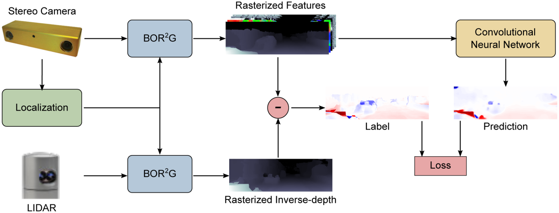
Machine learning data-flow pipeline. To train our network, we create separate stereo-camera and laser dense reconstructions, using the techniques discussed in Sections 3–5. We create GT data by subtracting the rasterized inverse-depth images from each reconstruction. The neural network trains on rasterized feature images (see Figure 11) to learn to generalize the GT error in new scenes.

6.1. Mesh features

Many works in the deep learning literature deal with RGB images and thus operate in two dimensions. However, as our problem formulation assumes that a dense 3D model is available, we can extract a much richer set of features from the reconstruction. Our system builds on the method proposed by Tanner et al. (2018), where mesh features are projected into sequences of 2D images. This method enables the use of established CNN architectures, while still leveraging the geometric information that meshes contain.

6.1.1. Feature creation

To extract dense 2D features suitable for a CNN, we begin by using OpenGL Shading Language (GLSL) to “fly” a virtual camera through the 3D models. Our vertex shader transforms the 3D model’s vertices into the camera reference frame to compute the depth of each vertex and the normalized camera vector. These camera-frame points are then grouped into triangles and passed along to a geometry shader that computes the triangle’s area, surface normal, and edge lengths. Finally, the fragment shader processes each of the preceding feature values and rasterizes them into individual pixels in feature images, as shown in Figure 11. This GLSL process enables us to extract six feature images: two per-pixel features (RGB and depth) and four per-triangle features (area, surface normal, edge length ratio, and surface-to-camera angle). Intuitively, the mesh-triangle-derived features contain a lot of information; they provide geometric cues that have been accumulated from multiple depth maps and fused into a 3D reconstruction by our system.

Fig. 11.

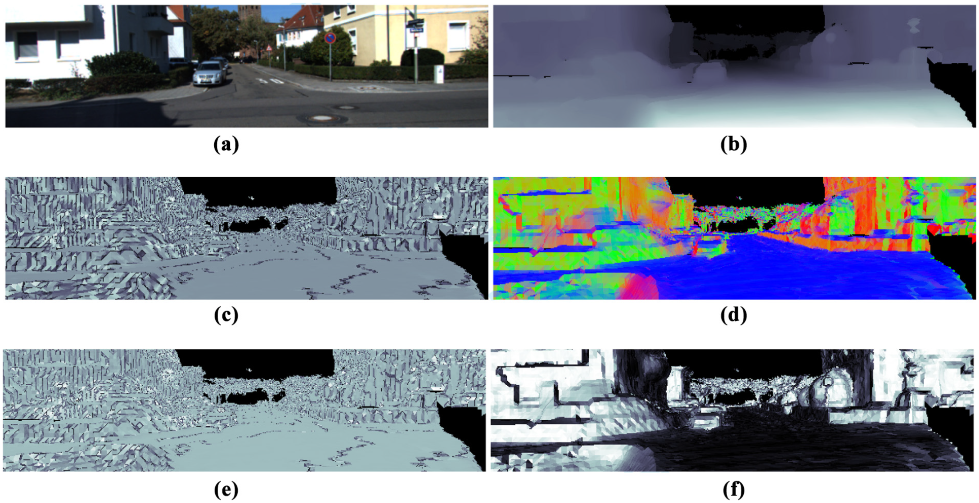
Example input features. An example frame from KITTI-VO and the corresponding features our GLSL pipeline currently extracts: (a) RGB image; (b) inverse-depth; (c) triangle area; (d) triangle surface normal; (e) triangle edge length ratios; (f) surface-to-camera angle. As our dense reconstructions provide a 3D model of our operating environment, we can extract a variety of features. The network has the potential to use these low-level features in its intermediate representation.

6.1.2. GT data

For a GT reference, we construct a mesh using the same reconstruction pipeline as used previously. The same virtual camera trajectory is used to create a sequence of feature images from both lower-quality (e.g., stereo-camera) and higher-quality (e.g., laser) reconstructions. Since the goal is to train a network to recognize errors in the lower-quality reconstruction, we must first compute GT errors with which to train the network. Rather than directly subtracting depths, we instead elect to use inverse-depth. In this way, the network is encouraged to emphasize errors in foreground objects, which are likely to have more detailed observable geometry compared with background surfaces. Specifically, we compute the per-pixel GT ( ${\mathrm{\Delta }}_{\mathrm{gt}}$ ) as

$${\mathrm{\Delta }}_{\mathrm{gt}}=\frac{1}{d_{\mathrm{lq}}}-\frac{1}{d_{\mathrm{hq}}}$$

(32)

where $d_{\mathrm{lq}}$ and $d_{\mathrm{hq}}$ are pixels in the depth-map features for the low-quality and high-quality reconstruction, respectively. An illustration of this is shown in Figure 12(c).

Fig. 12.

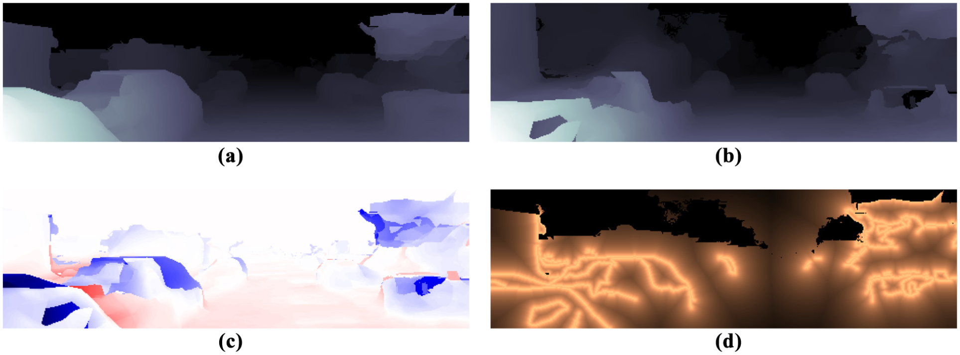
Illustration of the edge-based loss weighting used to train our neural network: (a) inverse-depth image of a lidar reconstruction; (b) inverse-depth image of a stereo-camera reconstruction; (c) GT error; (d) per-pixel loss weight. When learning to predict error for a scene (a), (b), edges are extracted from the GT error label (c) using the Canny edge detector, and a weighting based on the distance transform is computed (d). Brighter areas represent higher weights. The per-pixel losses (berHu, bilateral smoothness regularization) are scaled by this weight, increasing penalty especially around sharp edges. The black areas correspond to a weight of 0, where GT data is missing. Note the GT error (c) is signed: blue represents negative values (missing parts) and red represents positive values (extra parts).

6.2. Reconstruction error prediction

6.2.1. Network architecture

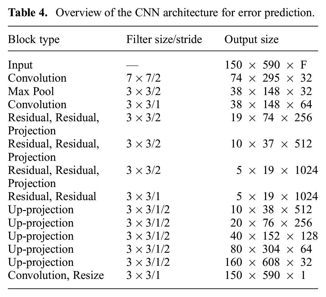
The architecture we employ in this article, similar to that proposed by Tanner et al. (2018), is based on the fully convolutional residual network (Laina et al. 2016) with concatenated ReLU activation functions on the intermediate layers (Shang et al. 2016). This network was designed to infer per-pixel depth from a single RGB image, a task highly correlated with our aim to compute estimated depth error given a set of feature inputs. In this work, the input layer is generalized to accept F input channels dependant on the number of active features used from the previous section. A notable addition is the U-Net-style (Ronneberger et al. 2015) skip connections between the encoder and the decoder. Table 4 gives a summary of the architecture. The encoder uses a series of residual blocks based on the ResNet-50 architecture (He et al. 2016), and the decoder uses the up-projection blocks proposed by Laina et al. (2016). The outputs of the residual blocks are padded and concatenated with the inputs to the up-projection blocks of corresponding scale. This architecture allows for high-frequency information (such as edges), to be more easily localized, since it is not compressed all the way through the encoder. The final layer is a simple $3\times 3$ convolutional layer which outputs real-valued estimates corresponding to the inverse-depth error at each pixel location.

Table 4.

Overview of the CNN architecture for error prediction.

Block type	Filter size/stride	Output size
Input	—	150 × 590 × F
Convolution	7×7/2	74 × 295 × 32
Max Pool	3×3/2	38 × 148 × 32
Convolution	3×3/1	38 × 148 × 64
Residual, Residual,Projection	3×3/2	19 × 74 × 256
Residual, Residual,Projection	3×3/2	10 × 37 × 512
Residual, Residual,Projection	3×3/2	5 × 19 × 1024
Residual, Residual	3×3/1	5 × 19 × 1024
Up-projection	3×3/1/2	10 × 38 × 512
Up-projection	3×3/1/2	20 × 76 × 256
Up-projection	3×3/1/2	40 × 152 × 128
Up-projection	3×3/1/2	80 × 304 × 64
Up-projection	3×3/1/2	160 × 608 × 32
Convolution, Resize	3×3/1	150 × 590 × 1

6.2.2. Generalization capacity

To be able to deploy a learned CNN to new meshes created without a high-fidelity sensor, we need our network to generalize to unseen data. To this end, three techniques are employed: cropping, downsampling, and weight regularization. First, we randomly perturb and crop all input feature images before providing them to the network. After each epoch of training (i.e., the network has viewed all the training images), the next epoch will receive a slightly different cropped region of each input image. This prevents the network from associating a specific pixel location in the training data with its corresponding output.

Second, the feature maps are gradually downsampled via projection blocks (from ResNet-50) creating a bottleneck, thus reducing representational capacity. This also provides greater context to the convolutional filters in the later layers of the network by increasing the size of their receptive field.

Third, we implement an $L_2$ weight regularizer to further constrain the representational capacity by preventing the network from over-relying on the cost function at the expense of generalization performance.

6.2.3. Loss function

Several loss functions are widely used in machine learning applications. The $L_2$ norm is traditionally popular because it heavily penalizes large errors and is smooth. However, unlike the $L_1$ norm, it has a near-zero gradient for small errors, thus is often unable to drive the error completely to zero. Over the years, researchers have proposed alternative norms that combine the “best” characteristics (based on application) of each of these norms. The Huber norm uses $L_2$ near the origin and $L_1$ elsewhere, while berHu uses the $L_1$ norm near the origin and the $L_2$ elsewhere (Owen 2007). We choose berHu as our cost function on the networks error prediction since the $L_1$ term places a higher penalty on small errors (when compared with Huber or $L_2$ ) while still providing strong penalties for larger errors. This is in contrast to regularizing depth maps where the Huber norm is more favorable to capture high gradient edges around objects (Newcombe et al. 2011b). These benefits were also observed in the related task of depth prediction Laina et al. (2016).

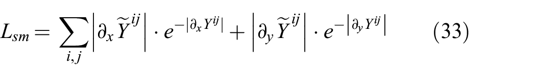
Similarly to Heise et al. (2013), Godard et al. (2017), and Mahjourian et al. (2018), an edge-aware smoothness loss is employed to further regularize the network. It essentially allows for discontinuities in CNN predictions ${\tilde{Y}}^{\mathrm{ij}}$ for each pixel ij, so long as there are corresponding discontinuities in the label $Y^{\mathrm{ij}}$ :

$$L_{\mathrm{sm}}=\sum _{i,j}\left|{\partial }_x{\tilde{Y}}^{\mathrm{ij}}\right|·e^{-\left|{\partial }_x{Y}^{\mathrm{ij}}\right|}+\left|{\partial }_y{\tilde{Y}}^{\mathrm{ij}}\right|·e^{-\left|{\partial }_y{Y}^{\mathrm{ij}}\right|}$$

(33)

Furthermore, inspired by the work of Ronneberger et al. (2015) on U-Nets, we use a loss-weighting mechanism based on the Euclidean distance transform (Felzenszwalb and Huttenlocher 2004) to give more importance to edge pixels when regressing to the error in depth (Figure 12). We first extract Canny edges (Canny 1986) from the GT labels. Based on these edges, we then compute the per-pixel weights as

$$\begin{array}{c}{d}^{\mathrm{ij}}=\ln (1+\mathrm{EDT}(i,j))\hfill \\ \multicolumn{1}{c}{w^{\mathrm{ij}}=(w_{\max }-w_{\min })*(1-\frac{d^{\mathrm{ij}}}{\underset{i,j}{max}{d}^{\mathrm{ij}}})+w_{\min }}\end{array}$$

(34)

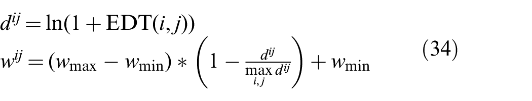
where $w^{\mathrm{ij}}$ is the loss weight for pixel ij, $\mathrm{EDT}(i,j)$ is the Euclidean distance transform at pixel ij, and $w_{\min }$ and $w_{\max }$ are the desired range of the per-pixel weight. We use $w_{\min }=0.1$ and $w_{\max }=5$ .

Finally, since the GT reconstructions might be missing some data, we allow for a per-pixel mask on the loss, to ignore pixels with unavailable data.

The final loss function can be written as

$$L=w_{\alpha }{L}_{\mathrm{reg}}+\sum _{\mathrm{ij}}{w}^{\mathrm{ij}}·(w_{\beta }{L}_{\mathrm{berHu}}^{\mathrm{ij}}+w_{\gamma }{L}_{\mathrm{sm}}^{\mathrm{ij}})$$

(35)

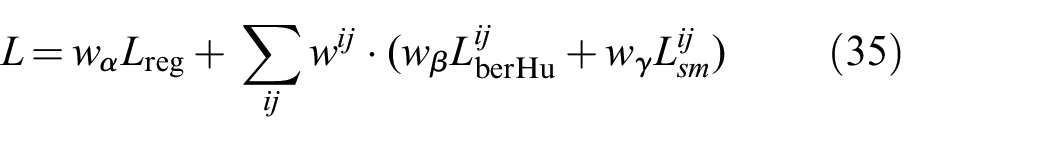
where $L_{\mathrm{reg}}$ is the weight regularization loss. We use $w_{\alpha }={10}^{-6}$ , $w_{\beta }=1$ , and $w_{\gamma }=1$ .

7. Results

This section provides an extensive analysis of our system, the parameters for which are provided in Table 3. Some parameters ( $\sigma$ , $\theta$ , $\tau$ ) are standard constants from the literature (Pock and Chambolle 2011). The parameters $\mu$ and $\lambda$ were empirically tuned. As discussed in Section 5.1.1, we found a constant $\mu$ value based on the sensor accuracy produced better results across a range of scenarios. When using multiple sensor modalities, we selected $\mu$ based on the least accurate sensor. We found $\lambda$ to be dependent on the sensor observation density (number of observations per voxel) and accuracy. Selecting too large $\lambda$ resulted in minimal changes to the quality of the reconstruction, but a very low $\lambda$ deletes too many surfaces. If the same platform is used with a similar sensor suite and vehicle velocity between data collections, as is the case in the KITTI dataset, then the same $\lambda$ is valid for all data collections.

In the first portion of our results, we present how our system’s reconstruction quality compares with prior work (Stanford Burghers of Calais and Imperial College ICL-NUIM). Next, we demonstrate its performance on our Oxford Broad Street dataset, that we release with this paper. Then, we use the publicly available KITTI dataset (Geiger et al. 2012) to evaluate the reconstruction performance of stereo-only, laser-only, and multi-sensor fusion methods. Finally, we use the KITTI dataset to present additional improvements that can be made to stereo-only reconstructions, when using a CNN trained on laser data.

Three KITTI sequences (00, 05, and 06) were selected based on their length, number of loop closures, and urban structure visible throughout the sequences. A summary of the physical scale of each is provided in Table 2.

The dense fusion and reconstruction experiments were performed on a GeForce GTX TITAN with 6 GB memory. The CNN mesh correction experiments were performed on a Tesla K80 with 12 GB memory.

Pose estimation was processed in real time (20 Hz); depth-map estimates (1 Hz), data fusion (5 Hz depth maps, 10 Hz Velodyne), and CNN post-processing (12 Hz) were at interactive rates; while the regularization could only be achieved via an off-line process since it required multiple minutes to converge in each scenario (see Table 5). With these timing requirements, we use this reconstruction (depth map and laser fusion) pipeline in real-time mobile-robotics applications, but then further improve the reconstructions via regularization as a part of the “dream state” robot maintenance between trials. We prefer to create small local maps (as used by Stewart and Newman (2012) and Maddern et al. (2014)). However, we describe in this section the utility of improving reconstructions after incorporating the loop closures when revisiting a location. After a loop closure, the dense reconstruction may be updated in real-time via graph deformation (Whelan et al. 2014) although some voxel historical data is lost in this process (voxels → mesh → deformed mesh → voxels).

Table 5.

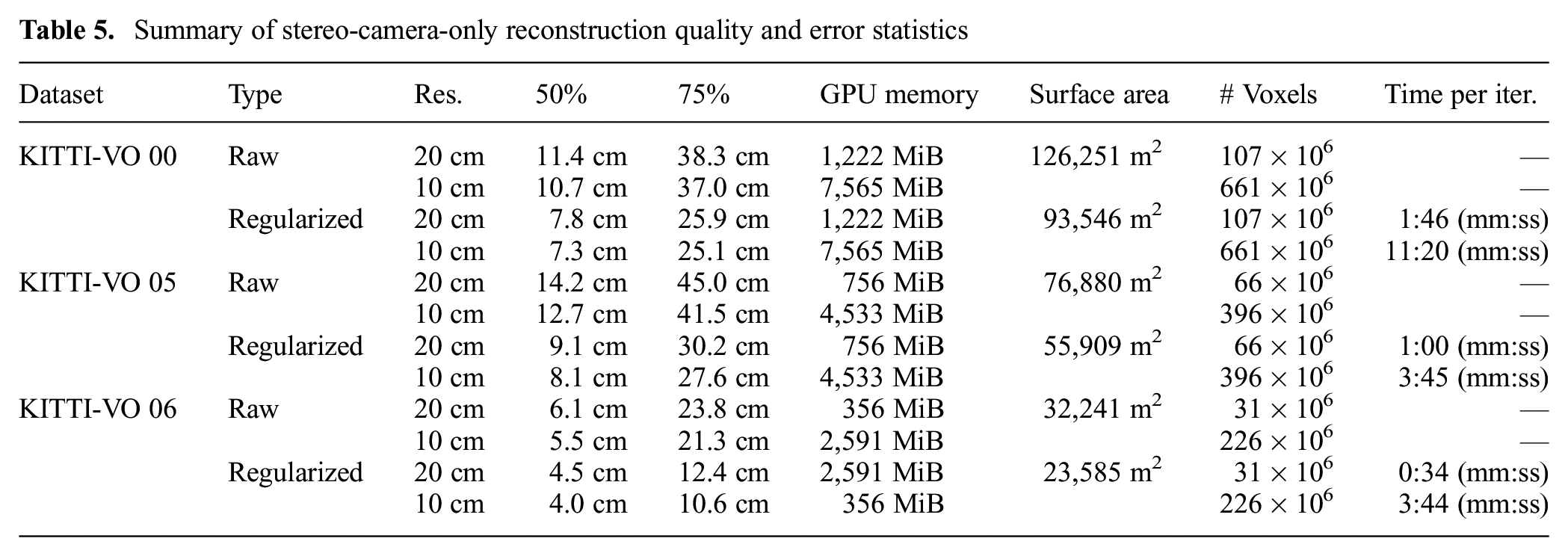
Summary of stereo-camera-only reconstruction quality and error statistics

Dataset	Type	Res.	50%	75%	GPU memory	Surface area	# Voxels	Time per iter.
KITTI-VO 00	Raw	20 cm	11.4 cm	38.3 cm	1,222 MiB	126,251 m2	107×106	—
		10 cm	10.7 cm	37.0 cm	7,565 MiB		661×106	—
	Regularized	20 cm	7.8 cm	25.9 cm	1,222 MiB	93,546 m2	107×106	1:46 (mm:ss)
		10 cm	7.3 cm	25.1 cm	7,565 MiB		661×106	11:20 (mm:ss)
KITTI-VO 05	Raw	20 cm	14.2 cm	45.0 cm	756 MiB	76,880 m2	66×106	—
		10 cm	12.7 cm	41.5 cm	4,533 MiB		396×106	—
	Regularized	20 cm	9.1 cm	30.2 cm	756 MiB	55,909 m2	66×106	1:00 (mm:ss)
		10 cm	8.1 cm	27.6 cm	4,533 MiB		396×106	3:45 (mm:ss)
KITTI-VO 06	Raw	20 cm	6.1 cm	23.8 cm	356 MiB	32,241 m2	31×106	—
		10 cm	5.5 cm	21.3 cm	2,591 MiB		226×106	—
	Regularized	20 cm	4.5 cm	12.4 cm	2,591 MiB	23,585 m2	31×106	0:34 (mm:ss)
		10 cm	4.0 cm	10.6 cm	356 MiB		226×106	3:44 (mm:ss)

7.1. Imperial College ICL-NUIM

We first evaluated the performance of our dense reconstruction pipeline (fusion and regularization) with the augmented Imperial College ICL-NUIM dataset (Choi et al. 2015). The original dataset (Handa et al. 2014) provided a set of indoor scenarios with sequences of GT 3D models, camera poses, and RGB-D images. Choi et al. (2015) augmented the dataset by applying lens and depth distortion models to make the input more similar to that of real-world data.

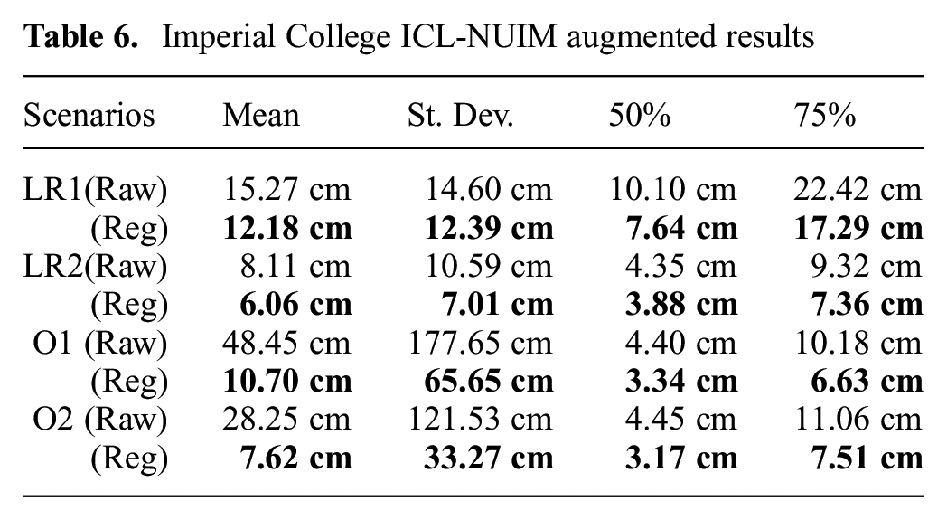
A summary of our reconstruction results are presented in Table 6. The median reconstruction error of the raw fused model ranged from 4.35 to 10.10 cm. The regularizer reduced error by 24% to 29%, with final median errors between 3.17 and 7.64 cm. The absolute error metrics are not as important as the fact that the regularizer consistently reduced the reconstruction errors: a theme which repeats throughout the quantitative results presented in this section.

Table 6.

Imperial College ICL-NUIM augmented results

Scenarios	Mean	St. Dev.	50%	75%
LR1(Raw)	15.27 cm	14.60 cm	10.10 cm	22.42 cm
(Reg)	12.18 cm	12.39 cm	7.64 cm	17.29 cm
LR2(Raw)	8.11 cm	10.59 cm	4.35 cm	9.32 cm
(Reg)	6.06 cm	7.01 cm	3.88 cm	7.36 cm
O1 (Raw)	48.45 cm	177.65 cm	4.40 cm	10.18 cm
(Reg)	10.70 cm	65.65 cm	3.34 cm	6.63 cm
O2 (Raw)	28.25 cm	121.53 cm	4.45 cm	11.06 cm
(Reg)	7.62 cm	33.27 cm	3.17 cm	7.51 cm

7.2. Stanford Burghers of Calais

We first validate that our dense-fusion system creates high-quality reconstructions with the standard Stanford Burghers of Calais RGB-D dataset (Zhou and Koltun 2013). We performed a point-to-surface comparison between BOR²G ’s (0.5 cm voxels) and Zhou and Koltun’s (unknown voxel size) reconstructions. BOR²G ’s median reconstruction difference was 0.5 cm with a 1.0 cm 75-percentile difference. Note that this is a “difference” not an “error” metric as there is no GT data against which we can compare.

As can be seen in Figure 1, our level of detail compares favorable with the reconstructions by Zhou and Koltun (2013). We accurately depict folds in clothing, muscle tone, and facial features.

However, this does not reveal the full capabilities of our framework as the low-noise, high-observation, and small-scale RGB-D dataset does not require sophisticated 2D and 3D regularization to create high-quality reconstructions. We are not aware of any other system which both operates at scale and accepts a variety of sensor inputs, hence the remaining quantitative analysis compares only against GT data.

7.3. Oxford Broad Street dataset

In practice, we found dense reconstructions are the most complete and highest quality (with our mobile robotics platform) when fusing data from multiple Velodyne, SICK LMS-151, and stereo cameras using our own datasets. We are releasing such a dataset with this article to provide a realistic mobile-robotics platform with a variety of sensors, a few of which are prime candidates for GT when testing the accuracy of reconstructions with other sensors. For example, the push-broom laser sensor (which excels at 3D urban reconstructions) can be used to compare the reconstruction quality of monocular versus stereo camera versus Velodyne versus a combination thereof.

This dataset is ideal to benchmark and evaluate large-scale dense reconstruction frameworks. It was collected in Oxford, UK, at midday, thus it provides a representative urban environment with numerous pedestrians, bicycles, and vehicles visible to all sensors throughout the 1.6 km trajectory (Figure 13).

Fig. 13.

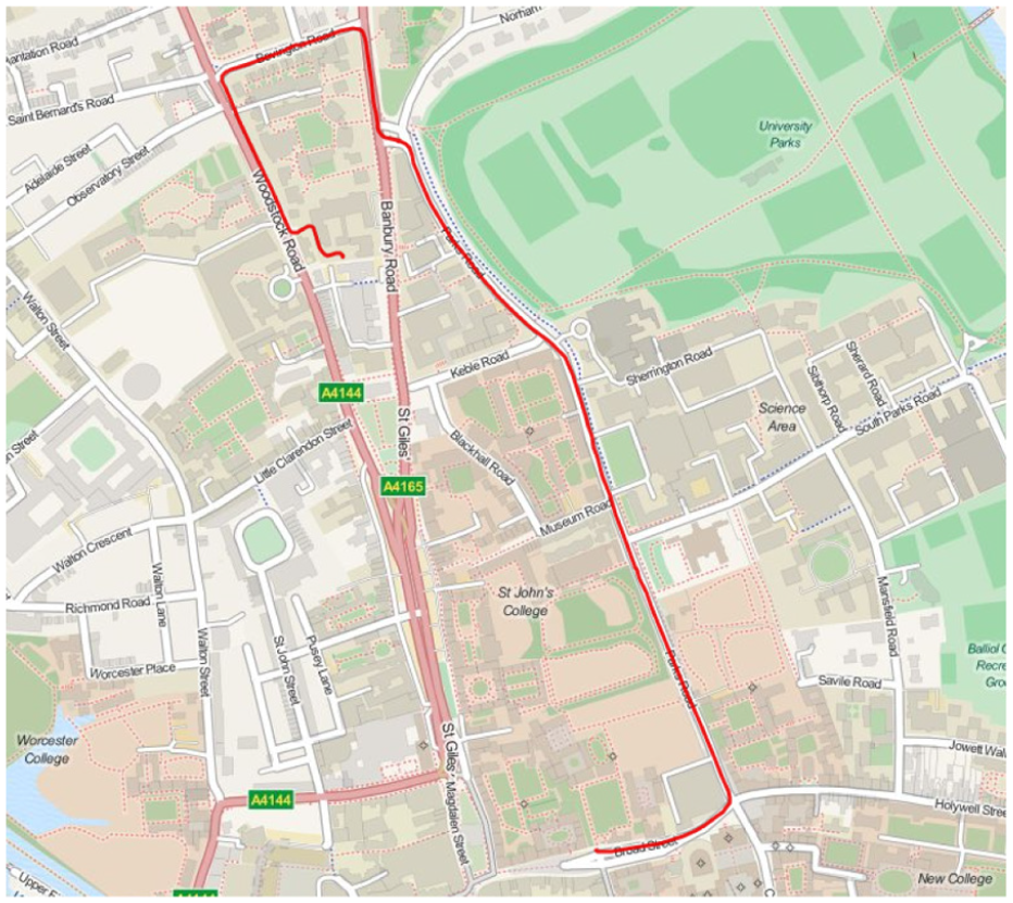
GPS trace for the Oxford Broad Street dataset. The dataset includes data from 1× Bumblebee XB3, 1× Bumblebee2, 4× Grasshopper2, 2× Velodyne HDL-32E lidar, and 3× SICK LMS-151 lidar sensors.

It includes data from the following sensors which collectively provide a continuous 360° view around the vehicle:

• 1× Point Grey Bumblebee XB3 stereo camera (color);

• 1× Point Grey Bumblebee2 stereo camera (grayscale);

• 4× Point Grey Grasshopper2 monocular cameras (color, fisheye lens);

• 2× Velodyne HDL-32E 3D lidars;

• 3× SICK LMS-151 2D lidars.

In addition, the following is provided to aid in processing the raw sensor data:

• optimized $\mathbb{S}\mathbb{E}(3)$ vehicle trajectory;

• undistorted, rectified stereo image pairs;

• undistorted mono images;

• camera intrinsics;

• extrinsic $\mathbb{S}\mathbb{E}(3)$ transforms for all sensors.

Finally, we provide example depth maps, using the techniques described in this article, for the Bumblebee XB3 to enable users to rapidly utilize the dataset with their existing dense reconstruction pipelines.

All data is stored in a similar format as KITTI along with MATLAB development toolkit. Videos of the included data are available at http://ori.ox.ac.uk/dense-reconstruction-dataset/.

For brevity, we provide more detailed analysis of the stereo-only, laser-only, and multi-sensor fusion performance on the KITTI dataset in the following subsections. However, an example Velodyne-based reconstruction of a small segment of this dataset is shown in Figure 2 and a larger qualitative analysis is included in the Supplemental Material video.

7.4. KITTI stereo-only reconstruction analysis

In addition to traditional qualitative analysis, KITTI stereo-only reconstructions may be quantitatively analyzed by using laser data as GT. We consolidated all Velodyne HDL-64E laser scans into a single reference frame using poses provided by ORB-SLAM2. We found that KITTI’s GT GPS/IMU poses were not accurate enough to produce high-quality dense reconstructions, in particular when revisiting regions. There was as much as 3 m of drift from one pass of a region to the second pass with the KITTI GT poses, while ORB-SLAM2 poses were accurate within a few centimeters.

The following three subsections perform analysis on the stereo-only reconstruction performance for SDF versus histogram data terms, comparing multiple stereo camera passes through the same environment, and the quantitative quality of 7.3 km of stereo-only reconstructions.

7.4.1. SDF versus histogram data terms

Zach (2008) demonstrated the superior histogram data term performance in small-scale, object-centered scenarios. We compare SDF and histogram optimization performance so dense-reconstruction system developers may make an informed decision based on their target application.

After fusing stereo-based depth images into the voxel grid, the resulting reconstruction is indeed noisy, as shown in Figure 14. The 2D TGV² regularizer significantly reduced the noise in the input depth maps, but passively-generated depth maps inherently must infer depth of large portions of the image.

Fig. 14.

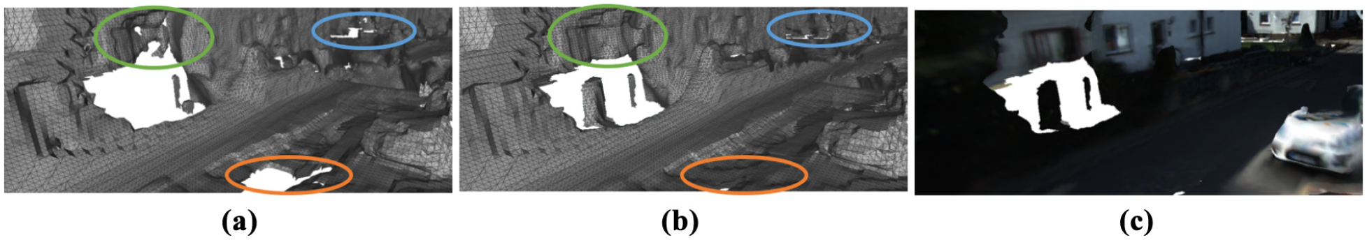
Comparison of reconstruction improvement with histogram and SDF data terms on stereo-camera-only reconstructions: (a) raw reconstruction; (b) histogram data term reconstruction; (c) SDF data term reconstruction; (d) final colored reconstruction. Both optimization methods noticeably smooth the surfaces (e.g., buildings, trees, automobiles) while also removing low-certainty surfaces (e.g., speckled surface in the sky near the trees). The SDF data term qualitatively produces “smoother” surfaces, but quantitatively (Table 7) SDF and histogram methods are nearly indistinguishable.

Both the SDF and Histogram optimizers smooth the noisy surfaces (e.g., buildings) in the reconstruction, but the SDF regularizer subjectively appears to do a better job. When compared against GT in Table 7, the SDF and histogram optimizers are nearly indistinguishable: both reconstructions have a 5.9 cm median point-to-surface error with a 28 cm standard deviation.

Table 7.

SDF versus histogram regularized reconstruction errors

Fusion method	Median	75%	Std. Dev.
SDF	5.9 cm	21.0 cm	28.0 cm
Histogram	5.9 cm	21.5 cm	27.9 cm

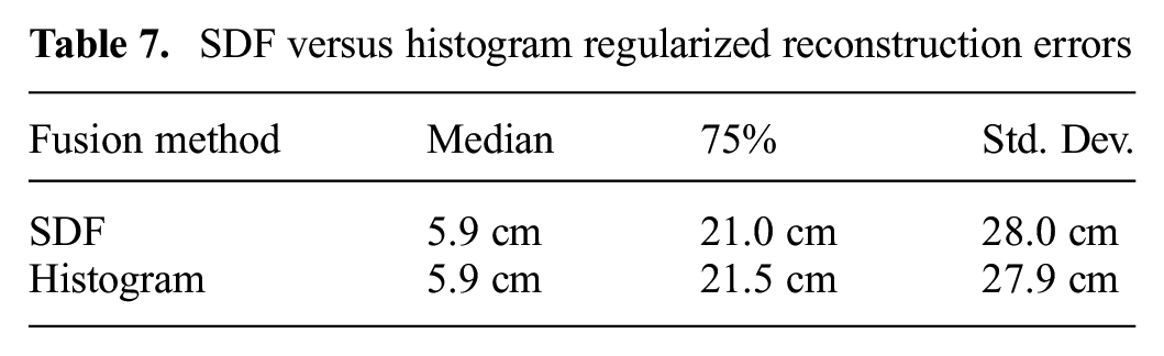
Based on Zach’s previous results, we initially expected the histogram to perform better. However, it appears that when a camera travels through the environment (rather than observing a single object from many angles) there are not enough observations of surfaces to provide a complete PDF in each voxel. Since the SDF regularizer is both simpler to implement, faster to execute, and provides similar results, we believe it can be a better choice for mobile-robotics platforms and we use it exclusively for the remainder of our experiments.

7.4.2. Multiple passes

In theory, revisiting a region should result in a more complete and accurate reconstruction, assuming one has accurate localization and loop closures. Noisy depth maps from the stereo camera preclude the traditional point-cloud alignment approaches used in Kinect Fusion-based approaches. However, ORB-SLAM2 provides accurate loop closures and locally consistent pose estimates.

In fact, ORB-SLAM2 performs better in our applications than did the GPS/INS GT: the latter resulted in trees and walls being observed in the middle of a road when revisiting a location.

In Figure 15, we compare the quality of reconstruction between a single and two passes of a region. The second pass noticeably improves the detail in previously observed surfaces and increases the surface area reconstructed by 11% (6,044 m² → 6,713 m²).

Fig. 15.

Comparison of fusion after two passes of the same region: (a) stereo camera pass 1; (b) stereo camera pass 2; (c) final colored reconstruction. The second pass results in a more complete model since, with accurate localization, the stereo-camera depth maps observe surfaces from a slightly different angle and lighting conditions. The first pass reconstructed 6,044 m², while the second pass increased that by 11% to 6,713 m². Note that the hole in the center-left of the image is due to object occlusions at the viewing angle of the input stereo images.

7.4.3. Full-length KITTI-VO error metrics

Using only the stereo camera as input, we first processed all three KITTI-VO with 10 cm voxels and compared the dense reconstruction model, both before and after regularization, to the laser scans. In these large-scale reconstructions, the compressed voxel grid structure provides efficient fusion performance while vastly increasing the size of reconstructions. For the same amount of GPU memory, the conventional voxel grid was only able to process 205 m, in stark contrast to the 1.6 km reconstructed with the HVG: though that may be extended to an infinite-size reconstruction by utilizing bidirectional GPU–CPU streaming.

As shown in Table 5, the SDF regularizer reduced the median error by 27% to 36%, the 75-percentile error by 32% to 50%, and the surface area by 26%. The final median error for the scenarios varied between 4.0 cm and 8.1 cm.

In Figure 16, it becomes clear that errors in the initial “raw” fusion largely come from false surfaces created in the input depth map caused by sharp discontinuities in the original image. The SDF regularizer removes many of these surfaces, which dominate the tail of the histogram plots and are visible as red points in the point-cloud plots.

Fig. 16.

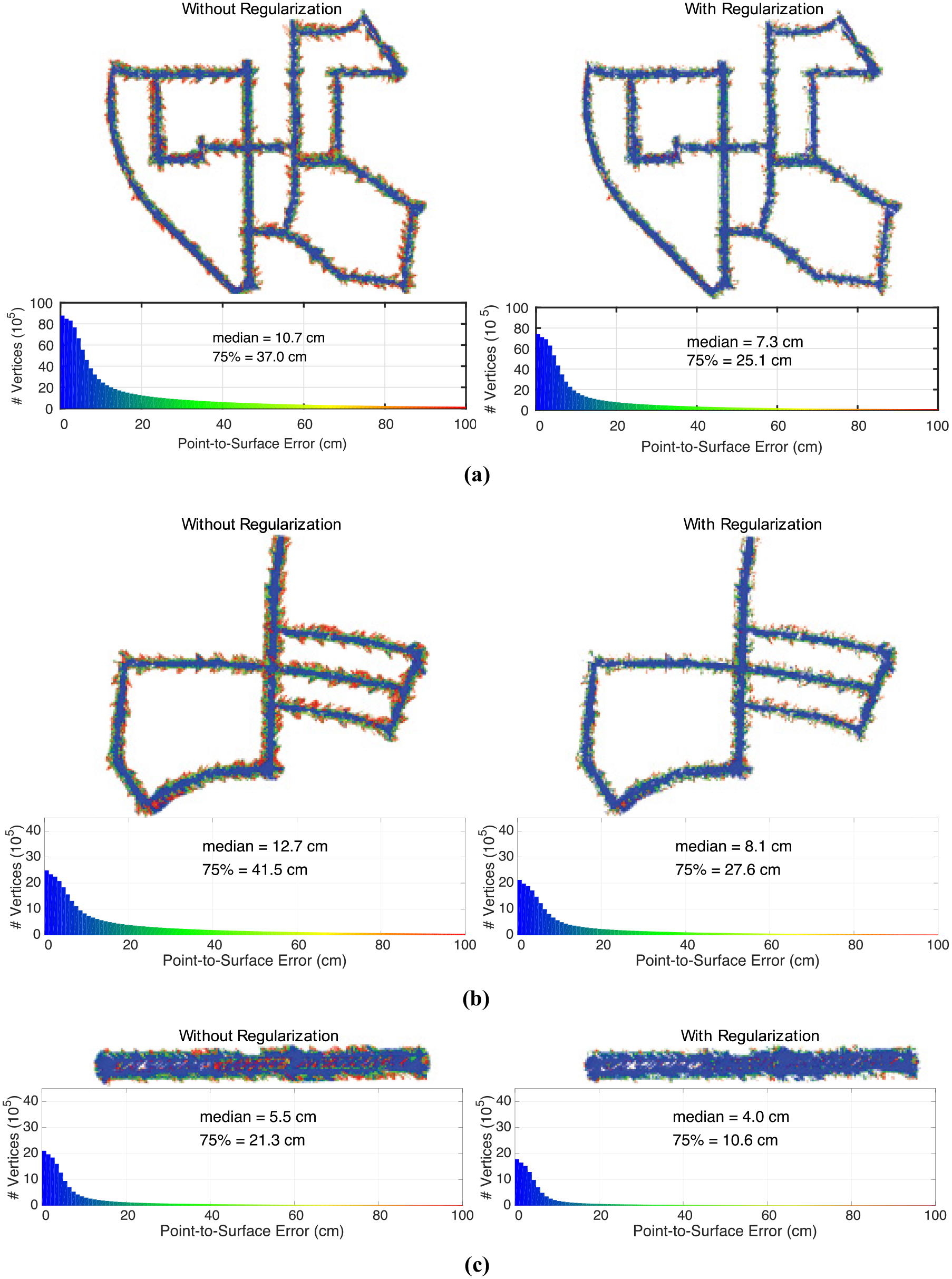
A summary of the stereo-camera-only dense reconstruction quality for three scenarios from the KITTI-VO public benchmark dataset. (a) KITTI-VO 00: stereo camera reconstruction error metrics. (b) KITTI-VO 05: stereo camera reconstruction error metrics. (c) KITTI-VO 06: stereo camera reconstruction error metrics. The left-hand side are the results before regularization and the right-hand side are after regularization. Above each histogram of point-to-surface errors are the top view, colored reconstruction errors corresponding to the same colors in the histogram. Note that the regularizer reduces reconstruction error by approximately a third, primarily by removing uncertain surfaces, as can be seen when you contrast the raw (left) and regularized (right) reconstruction errors.

When processed at 20 cm voxel resolution, the results are similar, though with slightly higher error metrics, as indicated by Table 5. However, even though the spatial resolution was reduced by a factor of two (and memory requirements by a factor of eight), the final reconstruction accuracy was only reduced by about 10%. This is because the urban environments are largely dominated by planar objects (e.g., roads, building façades) which, by the very nature of SDF, can be near-perfectly reconstructed with coarse voxels. Smaller voxels are only beneficial in regions with fine detail (e.g., automobiles, steps, curb).

Figure 17 shows the bird’s-eye view of each sequence with representative snapshots of the 10 cm stereo-camera-only reconstructions. To illustrate the quality, we selected several snapshots from camera viewpoints offset in both translation and rotation to the original stereo camera position, thereby providing a depiction of the 3D structure. Overall, the reconstructions are quite visually appealing; however, some artifacts such as holes are persistent in regions with poor texture or with large changes in illumination. This is an expected result since, in these cases, no depth map can be accurately inferred.

Fig. 17.

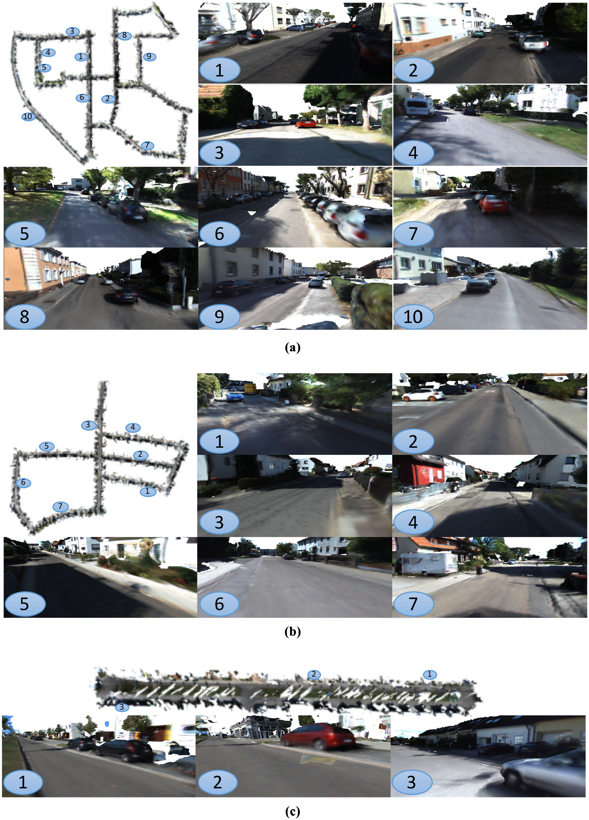
A few representative sample images for various points of view (offset from the original camera’s position) along each trajectory. (a) KITTI-VO 00: stereo camera reconstruction samples. (b) KITTI-VO 05: stereo camera reconstruction samples. (c) KITTI-VO 06: stereo camera reconstruction samples. These are not dataset images, but rather they are reconstructed 3D models generated from the full sequence of stereo pairs. All samples are of the final regularized reconstruction with 10 cm voxels using only stereo images as the input.

Fig. 18.

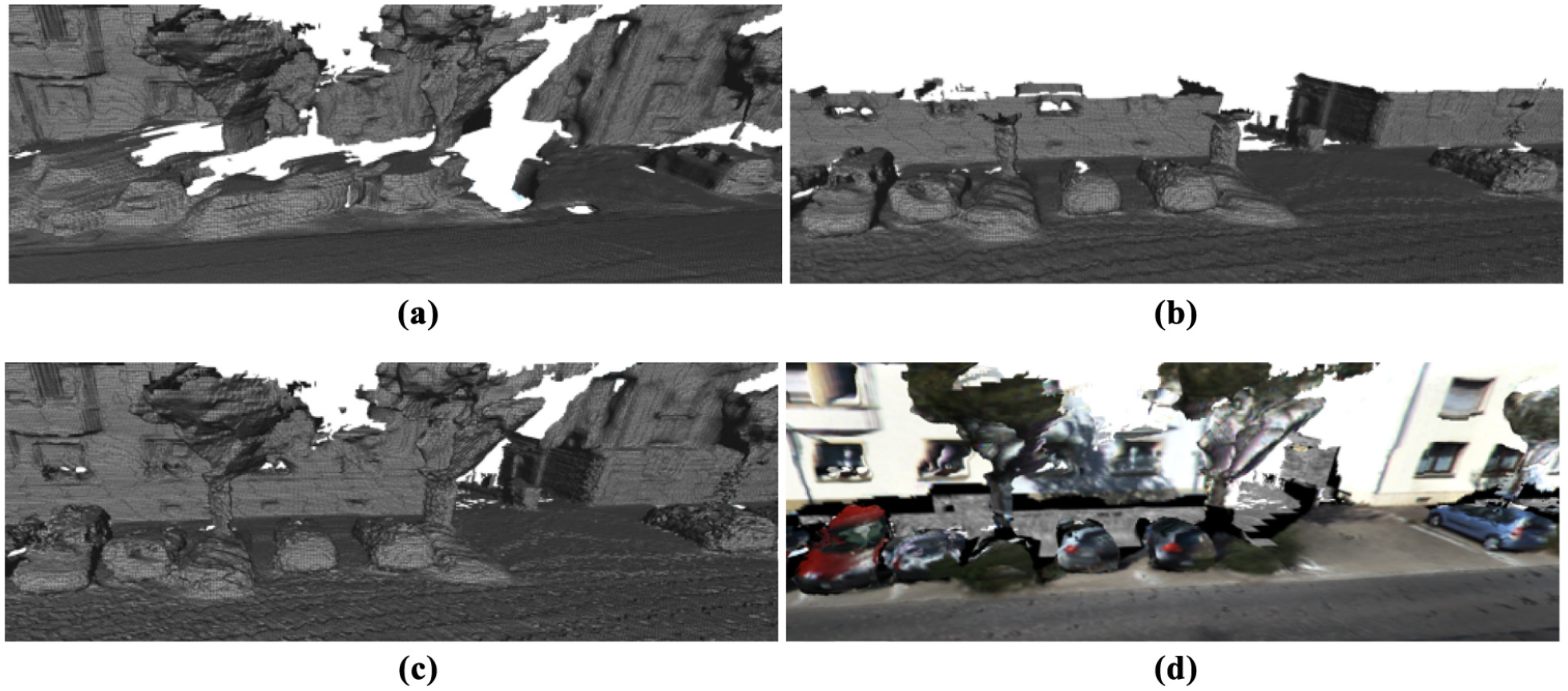
Comparison of reconstruction quality with (a) laser only, (b) stereo-camera only, (c) stereo-camera after CNN correction, and (d) final colored reconstruction. The correction step results in meshes with more coverage, though some areas (such as behind the parked cars) are occluded from the camera and therefore are not corrected. A less-obvious fix can be noticed in the road, where the uneven surface in (b), owing to the shadows in the original images, is smoothed in (c).

7.5 KITTI multi-sensor reconstruction analysis

Many mobile platforms have a variety of different sensors, yet conventionally much dense reconstruction work is isolated to a single sensor, and almost exclusively a camera of some sort (RGB-D, monocular, or stereo). The KITTI dataset provides both camera images and Velodyne laser scans, so we decided to see what quality of reconstructions could be achieved by fusing data from both sensors.

A snapshot of our qualitative results is given in Figure 19, but the supplemental material video provides a fly-through of each sequence to visualize the quality of our final regularized 3D reconstructions.

Fig. 19.

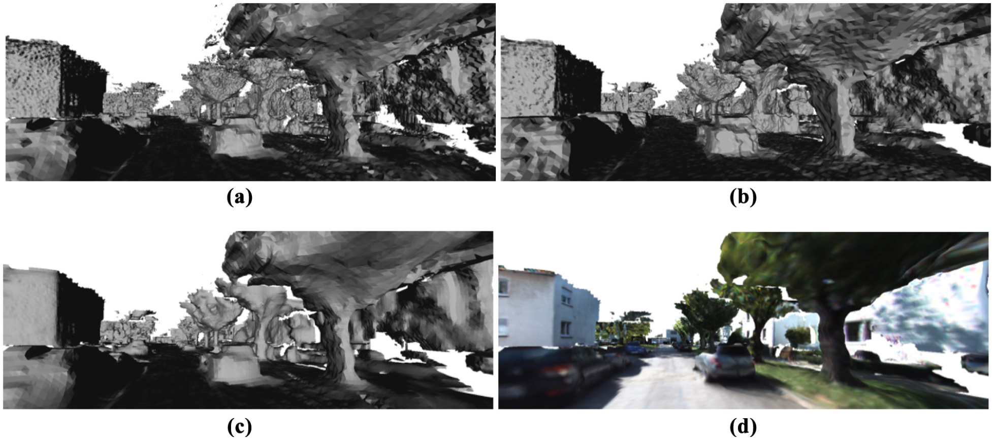
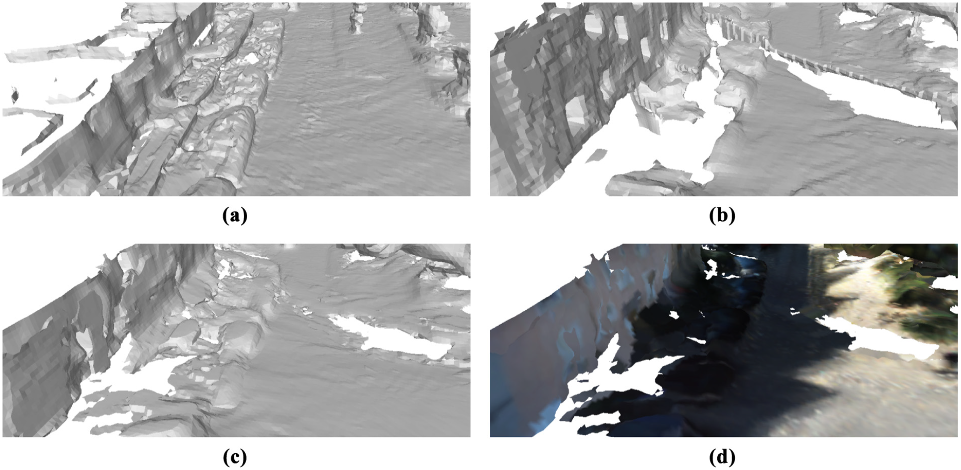
Comparison of reconstruction quality with (a) stereo-camera only, (b) laser only, (c) stereo-with-laser fusion, and (d) final colored reconstruction. The stereo camera has a higher field of view than the laser sensor (i.e., the building/trees are cut half way up in the laser reconstruction), but the laser sensor is much more accurate and can see into regions that were occluded for the stereo camera (e.g., behind the automobiles). Fusing data from both sensors into the same voxel grid produces a more comprehensive (Table 8) and higher-quality result than either sensor can achieve alone.

The stereo-camera-only reconstructions were moderately detailed, but a number of false surfaces were created between neighboring objects (e.g., automobiles, buildings) owing to the limitations of stereo-based depth maps. The camera reconstructions included the full height of the buildings, in contrast to the laser reconstructions that could only reconstruct the bottom 2.5 m of objects. However, the laser-only reconstruction was much more detailed and could see surfaces which were occluded to the camera (e.g., behind automobiles) because the Velodyne was mounted higher on the data-collection vehicle and it has a continuous 360° field of view.

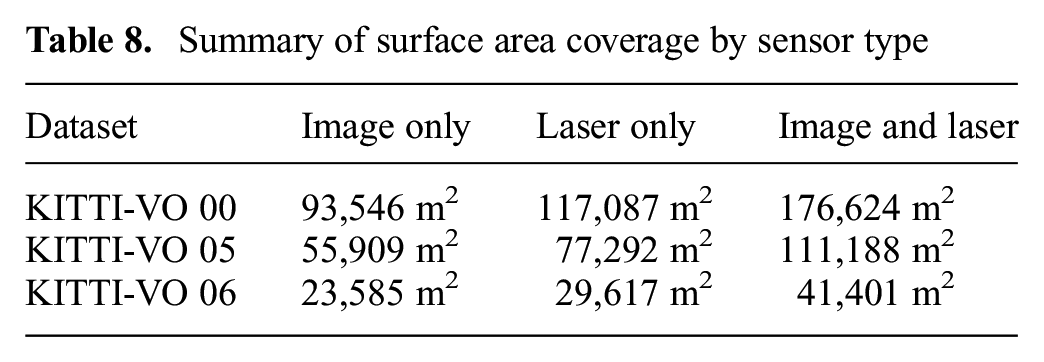
Figure 19c shows the combination of both sensors produced a reconstruction that was higher quality and more comprehensive. The comprehensiveness is measured in Table 8, where the multi-sensor fused reconstruction has 40% to 50% more surface area coverage than the best sensor was able to reconstruct by itself.

Table 8.

Summary of surface area coverage by sensor type

Dataset	Image only	Laser only	Image and laser
KITTI-VO 00	93,546 m2	117,087 m2	176,624 m2
KITTI-VO 05	55,909 m2	77,292 m2	111,188 m2
KITTI-VO 06	23,585 m2	29,617 m2	41,401 m2

7.6 Mesh correction with CNNs

Correcting meshes post hoc is particularly useful when dealing with reconstructions obtained in mobile robotics scenarios, where the amount of data is small relative to the surface area of the reconstruction.

In our experiments, we used a regularized laser reconstruction with 20 cm³ voxels as our high-quality prior, along with 20 cm³ regularized stereo-camera-only reconstructions to train the CNN described in Section 6. We generate mesh features along the original trajectories from each of the three KITTI sequences (00, 05, and 06), and train three models, one on each pair of sequences. When evaluating our approach on a sequence, we use the model trained on the other two sequences.

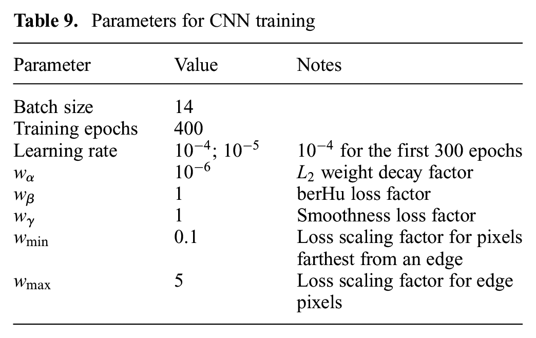
The network module was implemented in Python using the TensorFlow framework. The network weights were optimized using the ADAM solver (Kingma and Ba 2015) with a learning rate of ${10}^{-4}$ for 300 epochs over two of the sequences. At this point, the value of the loss function appears converged with variance coming form the stochasticity of the mini-batch sampling. To reduce this variance and confirm convergence, the optimization is run a further 100 epochs with the learning rate reduced to ${10}^{-5}$ . All training parameters are documented in Table 9.

Table 9.

Parameters for CNN training

Parameter	Value	Notes
Batch size	14
Training epochs	400
Learning rate	${10}^{-4}$ ; ${10}^{-5}$	${10}^{-4}$ for the first 300 epochs
$w_{\alpha }$	10−6	$L_2$ weight decay factor
$w_{\beta }$	1	berHu loss factor
$w_{\gamma }$	1	Smoothness loss factor
$w_{\min }$	0.1	Loss scaling factor for pixelsfarthest from an edge
$w_{\max }$	5	Loss scaling factor for edgepixels

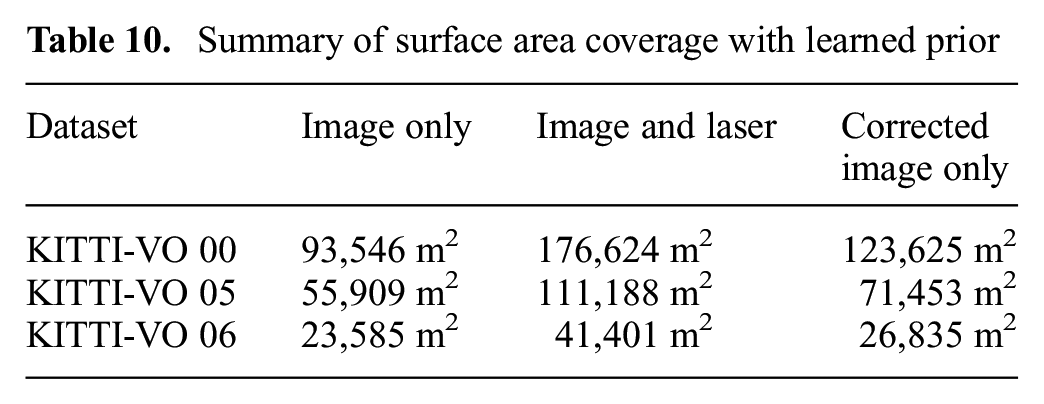
The reconstructions obtained by fusing laser and stereo-camera data are the most complete we can obtain given the sensor setup. As listed in Table 10, our learned correction closes the coverage gap between the stereo-camera reconstruction and the combined reconstruction by 18–36%, without increasing the metric error. The additional coverage is shown qualitatively in Figure 18.

Table 10.

Summary of surface area coverage with learned prior

Dataset	Image only	Image and laser	Correctedimage only
KITTI-VO 00	93,546 m2	176,624 m2	123,625 m2
KITTI-VO 05	55,909 m2	111,188 m2	71,453 m2
KITTI-VO 06	23,585 m2	41,401 m2	26,835 m2

7.7. EUROfusion Joint European Torus Reconstruction

We also demonstrate a very different practical application of our work at the Joint European Torus (JET), which is operated by the UK Atomic Energy Authority (UKAEA) under contract from the European Commission, and exploited by the EUROfusion consortium of European Fusion Laboratories. ¹

Together with the UKAEA remote maintenance division, Remote Applications in Challenging Environments (RACE), an inspection was carried out inside the JET device using the remote maintenance system (Figure 20), in order to collect lidar and camera data. Our inspection platform (the “NABU”) is equipped with two push-broom lidars that are used in the reconstruction (2.5 cm voxels), and a stereo camera used for visual odometry. We ran our pipeline on some of the data obtained, and Figure 21 shows the reconstruction. The recovered surface has a 287 m² area.

Fig. 20.

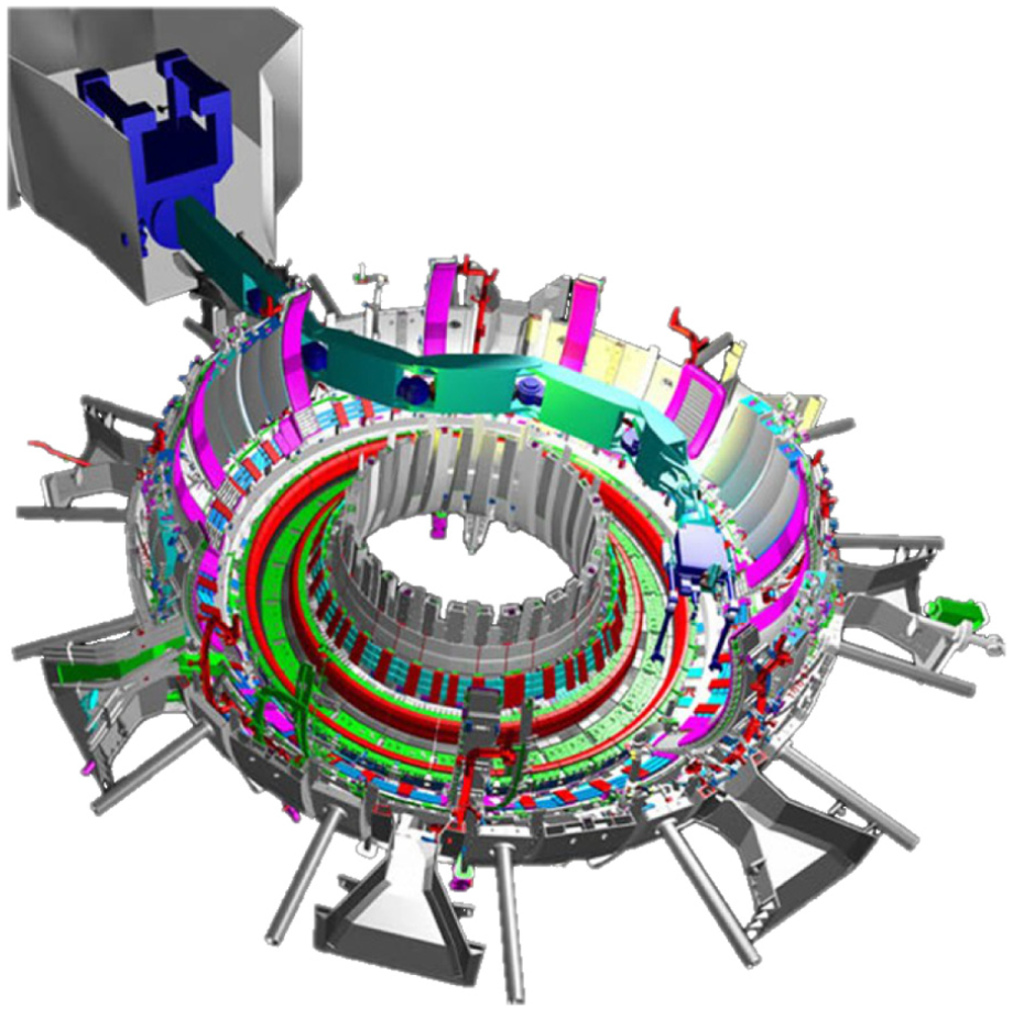
Schematic view of the JET fusion device, showing the remote maintenance systems (boom and mascot) deployed inside the torus. Image: EFDA-JET.

Fig. 21.

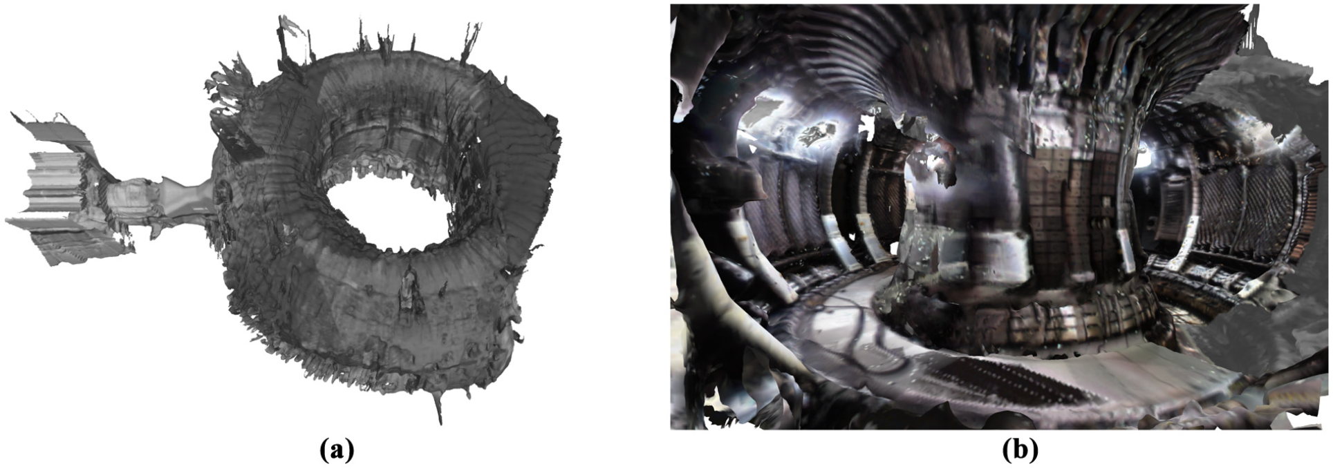
Two reconstructions of the JET fusion device: (a) outside view of JET (laser only); (b) inside view of JET (laser and stereo camera). This is a particularly challenging scenario, owing to the many reflective surfaces inside the reactor vessel. The laser scans covered about 75% of the torus, as well as part of the Tile Carrier Transfer Facility, shown on the far left in (a), used to gain access to the reactor vessel. In (b), we show a view inside JET from a laser and stereo camera reconstruction. Note that in the bottom right of the image, the reconstruction does not have color information, since that area was never in view of the camera. Instead, laser intensity is used to color that portion of the reconstruction.

The inside of the JET reactor vessel contains many reflective surfaces, which induce considerable noise in the laser measurements. This kind of scenario is particularly challenging, and benefits from our fusion and regularization components.

8. Conclusion

We have presented our state-of-the-art BOR²G dense mapping system for large-scale dense reconstructions. When compared with object-centered reconstructions, mobile-robotics applications have 3,100 times fewer depth observations per square meter, thus we utilized regularizers in both two and three dimensions to serve as priors that improve the reconstruction quality. We overcame the primary technical challenge of regularizing voxel data in the compressed 3D structure by redefining the gradient and divergence operators to account for the additional boundary conditions introduced by the data structure. This both enables regularization and prevents the regularizer from erroneously extrapolating surface data.

We know of no other dense reconstruction system that is quantitatively evaluated at such a large scale. When qualitatively compared with the Stanford Burghers of Calais RGB-D dataset, BOR²G reconstructed the same fine detail. For our large-scale reconstructions, we used the 3D lidar sensor as GT to evaluate the quality of our reconstructions, for different granularities, against 7.3 km of stereo-camera-only reconstructions. Our regularizer consistently reduced the reconstruction error metrics by a third, for a median accuracy of 7 cm over 173,040 m² of reconstructed area. Qualitatively, fusing both stereo-camera-based depth images with lidar data produces reconstructions that are both higher quality and more comprehensive than either sensor achieves independently. We demonstrated our system on a practical inspection task by producing a reconstruction of the EUROfusion JET.

We have shown how a CNN can be trained on historical high-fidelity data to learn a prior that can correct gross errors in meshes, such as holes in the road or cars. We have overcome the challenge of processing meshes with CNNs by rasterizing appearance and geometric features and applying 2D techniques. The learned CNN prior closes the gap in coverage by 18–36% without increasing the metric error.

Finally, we hope the release of our GT KITTI pointclouds, GT KITTI 3D models, and the comprehensive Oxford Broad Street dataset will become helpful tools of comparison for the community.