
Abstract
Natural environments are often filled with obstacles and disturbances. Traditional navigation and planning approaches normally depend on finding a traversable “free space” for robots to avoid unexpected contact or collision. We hypothesize that with a better understanding of the robot–obstacle interactions, these collisions and disturbances can be exploited as opportunities to improve robot locomotion in complex environments. In this article, we propose a novel obstacle disturbance selection (ODS) framework with the aim of allowing robots to actively select disturbances to achieve environment-aided locomotion. Using an empirically characterized relationship between leg–obstacle contact position and robot trajectory deviation, we simplify the representation of the obstacle-filled physical environment to a horizontal-plane disturbance force field. We then treat each robot leg as a “disturbance force selector” for prediction of obstacle-modulated robot dynamics. Combining the two representations provides analytical insights into the effects of gaits on legged traversal in cluttered environments. We illustrate the predictive power of the ODS framework by studying the horizontal-plane dynamics of a quadrupedal robot traversing an array of evenly-spaced cylindrical obstacles with both bounding and trotting gaits. Experiments corroborate numerical simulations that reveal the emergence of a stable equilibrium orientation in the face of repeated obstacle disturbances. The ODS reduction yields closed-form analytical predictions of the equilibrium position for different robot body aspect ratios, gait patterns, and obstacle spacings. We conclude with speculative remarks bearing on the prospects for novel ODS-based gait control schemes for shaping robot navigation in perturbation-rich environments.
1. Introduction
Existing research on robot navigation and path planning (Khatib, 1986; LaValle, 2006) has largely been premised on a clear distinction between a traversable “free space,” separated from the set of “obstacles” that can never be even touched. Indeed, because most available platforms lack any capability to cope with unanticipated mechanical contacts, robots generally rely heavily on active sensing to avoid engagement of any kind. However, as our increasingly capable robots begin to operate in more natural, less structured environments, it seems clear that this constraint must be relaxed, or even exploited.
We hypothesize that the disturbances from obstacles can be regarded as opportunities to enhance mobility in complex environments (Figure 1). Biological studies have demonstrated that animals (Kinsey and McBrayer, 2018; Kohlsdorf and Biewener, 2006; McInroe et al., 2016; Wilshin et al., 2017) can coordinate their appendages or body segments (Schiebel et al., 2019; Zhong et al., 2018) to adjust the timing and positions of environment engagement (Gart and Li, 2018; Gart et al., 2018; Li et al., 2015) to achieve effective locomotion. In analogy to the selected leg sequence timing in biological locomotors, Johnson and Koditschek (2013) demonstrated that with a human-programmed leg activation sequence, a hexapedal robot can jump up a vertical cliff by using its front legs to hook on the cliff edge while pushing its rear legs against the vertical surface. These studies suggested that with a better understanding of environment responses and interaction dynamics, robots could exploit obstacles and collisions to achieve environment-aided locomotion.

Natural terrains on Earth and in extraterrestrial environments are often filled with obstacles that generate large, repeated disturbances to robot locomotion. (A) Boulder field at Hickory Run State Park. Photo courtesy of Clyde. (B) Martian surface. Photo taken by NASA’s Curiosity Rover. (C) Log jam. Photo courtesy of Scampblog.
A key challenge in endowing robots with the ability to autonomously generate such environment-aided locomotion is the problem of conceptualizing how to even extract information about, much less exploit, these interaction opportunities from physical properties (e.g., shape, size, distribution) of the environment. On flat and rigid ground, robot dynamics can be modeled accurately (Blickhan, 1989; Brown and Loeb, 2000; Schmitt and Holmes, 2000), and numerous methods have been developed for control and planning on such simple terrain (De and Koditschek, 2018; Raibert, 1986). However, once the robots are allowed to interact with more complex environment (Li et al., 2010; Marvi et al., 2014; Qian and Goldman, 2015b; Qian et al., 2013), many simplified models and templates (Full and Koditschek, 1999) fail to capture the coupled dynamics, and previous control and planning methods are no longer applicable.
Gibson (1979) proposed the notion of environmental affordance as an agent’s acting to exploit an environmental structure in a manner favorable to some desired outcome. In the past few decades, there have been a number of biomechanics (Gart et al., 2019; Li et al., 2015; McInroe et al., 2016; Sane and Dickinson, 2001; Schiebel et al., 2019; Winter et al., 2012) and robotics (Arslan and Saranli, 2012; Bayraktaroglu and Blazevic, 2005; Byl and Tedrake, 2009; Curet et al., 2010; Kim et al., 2008; Qian and Goldman, 2015a; Qian et al., 2013; Rieser et al., 2019; Transeth et al., 2008; Winter et al., 2014) studies that began to reveal a wide variety of environmental affordances (Gibson, 1979) for locomotion, and how different locomotor morphology and kinematics allows exploitation of such affordances to effectively move through complex environments.
As a first step towards constructing a general framework of exploiting environmental affordance through gaits (Gibson, 1979), in this study we abstract the physical obstacles to treat them as the source of a horizontal-plane disturbance force field (Section 3.1). A previous study (Qian and Goldman, 2015b) on robot interaction with a single obstacle revealed that the change of robot orientation state after the interaction depended primarily on the initial fore–aft contact position on the obstacle. In this work, we expand this empirically characterized relationship to propose a disturbance field representation of horizontal-plane obstacle influences on robot dynamics. The values of the two-degree-of-freedom (2-DoF) disturbance field represent the direction and magnitude of fore–aft obstacle forces on the hip joint of a contacting robot leg.
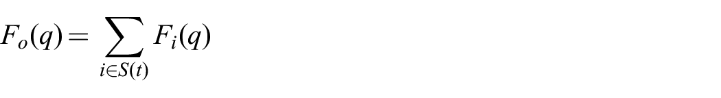
The disturbance field provides a map of available interaction forces in the given physical environment. That said, the total obstacle reaction forces on and the resulting dynamics of the center of mass (CoM) of a robot depend sensitively on the position and time of contact between robot legs and obstacles. In this article, we regard robot legs as a collection of disturbance selectors (Section 3.2), and we calculate the total interaction force exerted on the robot CoM by adding disturbance forces from each leg in contact with the obstacle. By coordinating leg movements and engaging its limbs with obstacles at different positions and times, a multi-legged robot can elicit a wide variety of dynamical effects from the same environment.
Combining the disturbance-field representation of environment and the disturbance-selector representation of the locomotor, our obstacle disturbance selection (ODS) framework provides a general method to predict robot dynamics under obstacle modulation. To validate our method, we construct a numerical model (Section 4) using the ODS framework. We study in both experiment (Section 2) and numerical simulation (Section 4) the dynamics of a quadrupedal robot, HQ-RHex (Figure 2A, Section 2.2), as it locomotes across an array of half-cylindrical obstacles (“logs”). Although a quadruped, a relatively simple form of multi-legged platform, is used to demonstrate the application of our framework in experiment (Section 2) and simulation (Section 4), we posit that the framework described in Section 3 is applicable to more general multi-legged platforms with different numbers of legs.
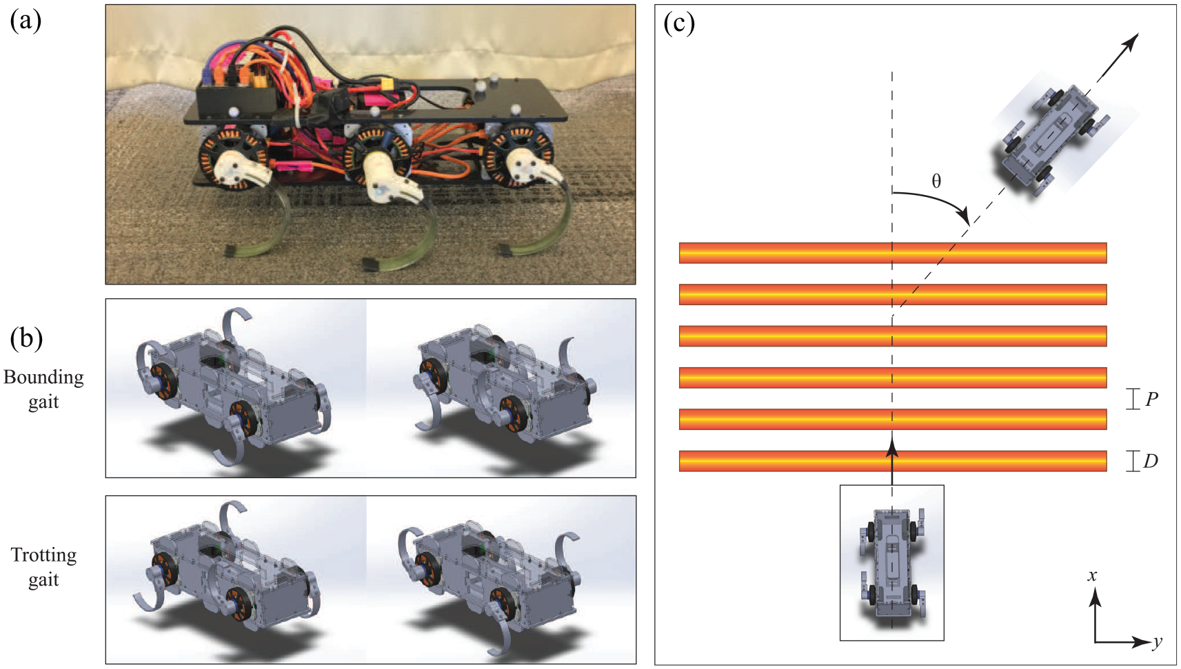
Experiment setup for exploring the effect of different gaits on robot traversal of a periodic obstacle field. (A) HQ-RHex, a small RHex-class (Saranli et al., 2001) robot. For experiments in this study we used a quadrupedal version of this robot by removing the two middle legs. (B) Two quadrupedal gaits were tested in the experiment, both of which involved two sets of two legs paired in phase, with the two pairs of legs in anti-phase. In bounding, two front legs are paired to move synchronously and then alternate with the two back legs; in trotting, two diagonal legs are paired and alternates with the other pair. (C) HQ-RHex’s instantaneous CoM positions (
We analyze the horizontal-plane dynamics of the HQ-RHex robot for two periodic gaits, a bound and a trot (Figure 2B). In both experiments and ODS-framework-derived numerical simulation, we find that the bounding robot exhibits a stable equilibrium state at a yaw angle of
Further analysis suggests that the emergence of this “locking angle” is a result of spatial period matching (Section 5) between the cyclic gait and the periodically structured environment. Using the spatial period matching principle, we demonstrate that the equilibrium orientation angle can be analytically predicted for a variety of obstacle spacings and robot body dimensions. In addition, the emergence of this passive stabilization mechanism from the simplified environments (periodic gaits in structured obstacle fields) suggests the possibility of active gait control schemes in more complex environments. We envision that by actively adapting gait sequences, a multi-legged robot can strategically select obstacle disturbances to achieve desired dynamics in cluttered environments (Section 6).
2. Obstacle modulation experiments
To begin to understand how robot dynamics changes under repeated obstacle disturbances, we performed locomotion experiments with a quadrupedal robot traversing across a field of evenly spaced obstacles. We systematically varied obstacle spacing and robot gait, and analyzed how these parameters affect the coupling between the robot and the environment.
2.1. Environment
The environment we used in this study was a simplified obstacle field with an array of half-cylindrical obstacles (“logs”) of diameter
The outer diameter
2.2.Robot
The robot used in this study, HQ-RHex (
As a first step to investigate the effect of gait patterns on robot dynamics under obstacle modulation, we tested the dynamics of HQ-RHex with two periodic gaits, bounding and trotting (Figure 2B). Bounding refers to the gait where two front legs move synchronously and two back legs move synchronously and out of phase with the front legs. Trotting refers to the gait where two diagonal legs move synchronously and out of phase with the other two legs.
2.3. Data collection and analysis
We performed 49 experiments with a bounding gait and 68 experiments with a trotting gait. We selected the initial fore–aft distance to ensure that the robot maintains the desired initial orientation and moves at least three complete stride cycles before entering the obstacle field. Each bounding trial started with the robot standing with a fore–aft distance of
We used a wireless remote joystick (Quanum i8) to set the stride frequency and gait pattern of the robot at the beginning of each trial. Once the trial started, the leg motors followed a desired angular position sequence generated based on the commanded stride frequency and gait pattern, and the robot traversed the obstacle-cluttered terrain in a feed-forward fashion without steering control. All changes in robot orientation, therefore, resulted from obstacle disturbances.
For each trial, the robot was set to a fixed stride frequency. Two different stride frequencies,
To track the dynamics of the robot during interaction with obstacles, we glued reflective markers (B
The initial orientation angle of the robot before it began interacting with the obstacle field,
2.4.Experiment observations
Robot trajectories measured from experiments are plotted in Figure 3A and C. We observed that with a bounding gait, despite the large variation in initial orientations the robot converged to traversing perpendicularly across the logs (
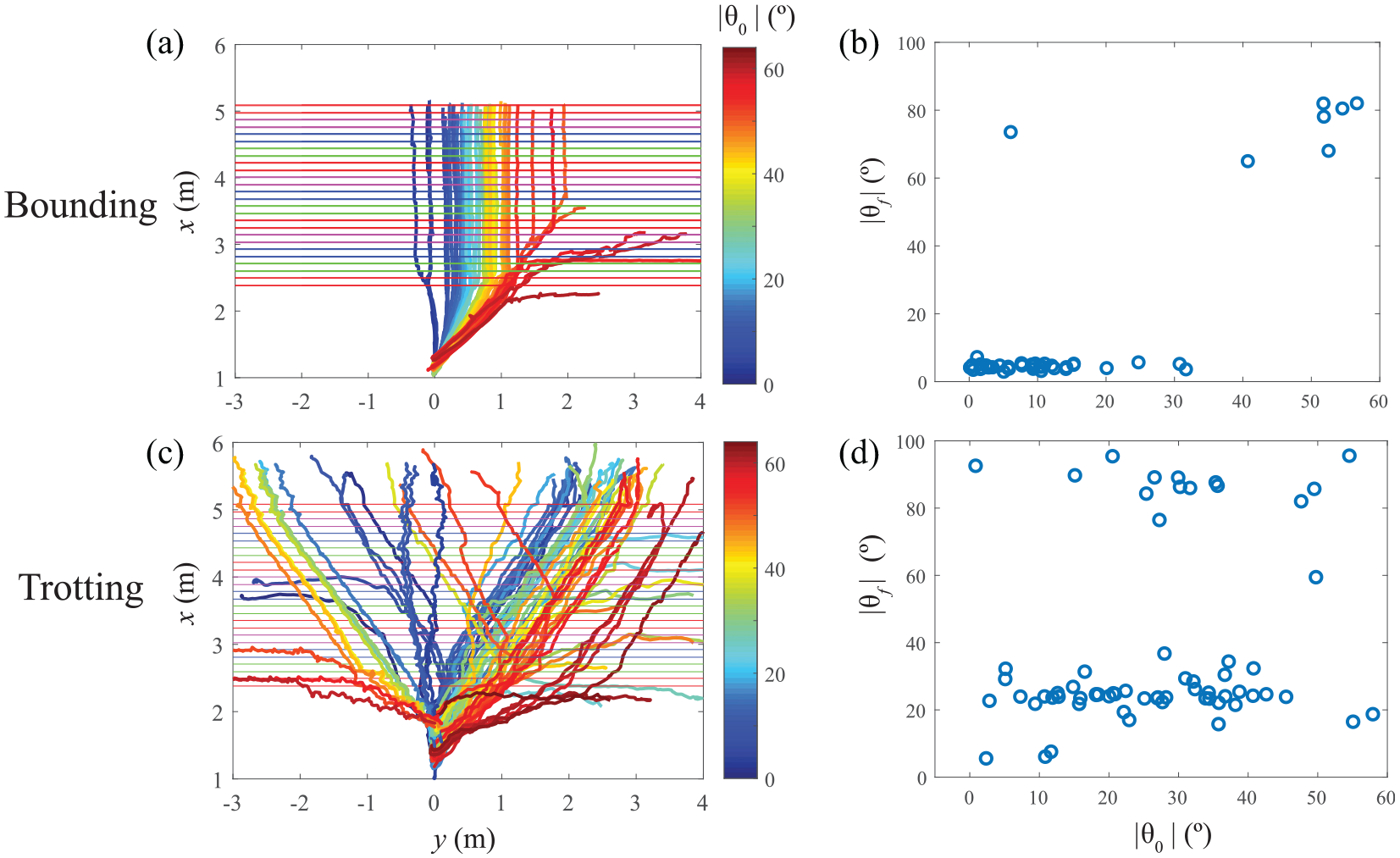
Robot trajectories and steady-state yaw angles measured from experiments. (A) Paths of the robot traversing across the obstacle field with a bounding gait. Colors represent different initial yaw angle magnitude. Horizontal lines represent the obstacles’ positions. Each obstacle was marked by a distinct color, with two horizontal lines representing the front and back edges. (B) Magnitude of the final yaw angle
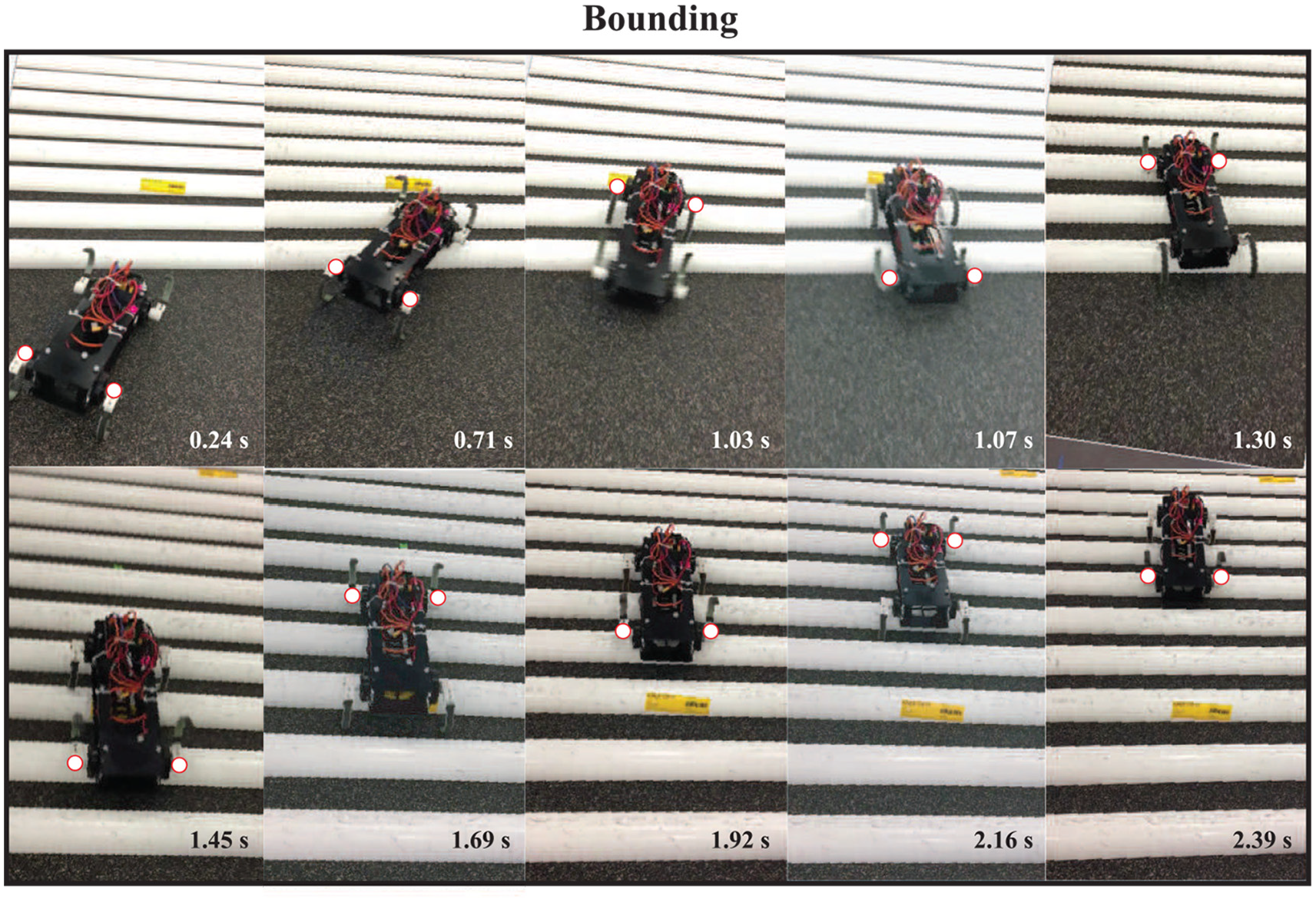
Sequence of images from a bounding experiment showing the robot orientation was locked to
With the trotting gait, however, the stabilized orientations were significantly different from those with the bounding gait. None of the trajectories (Figure 3C) converged to
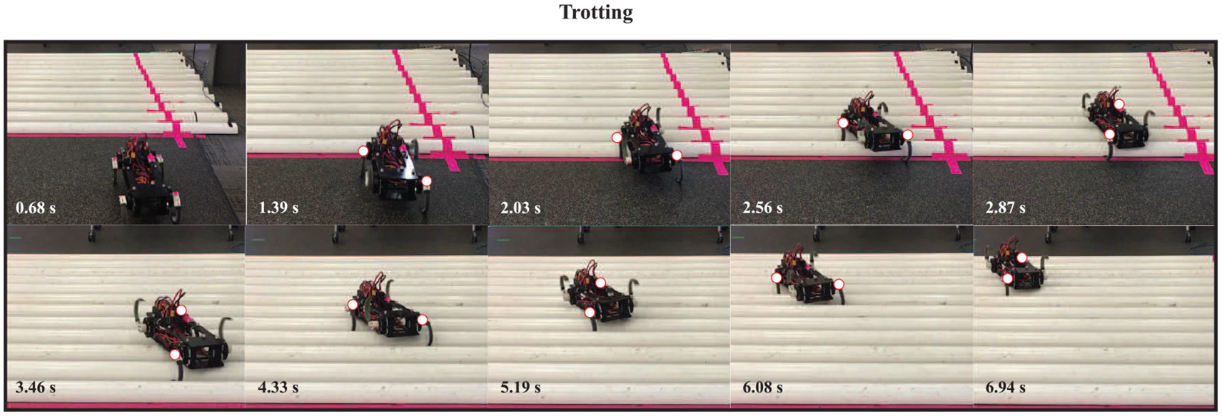
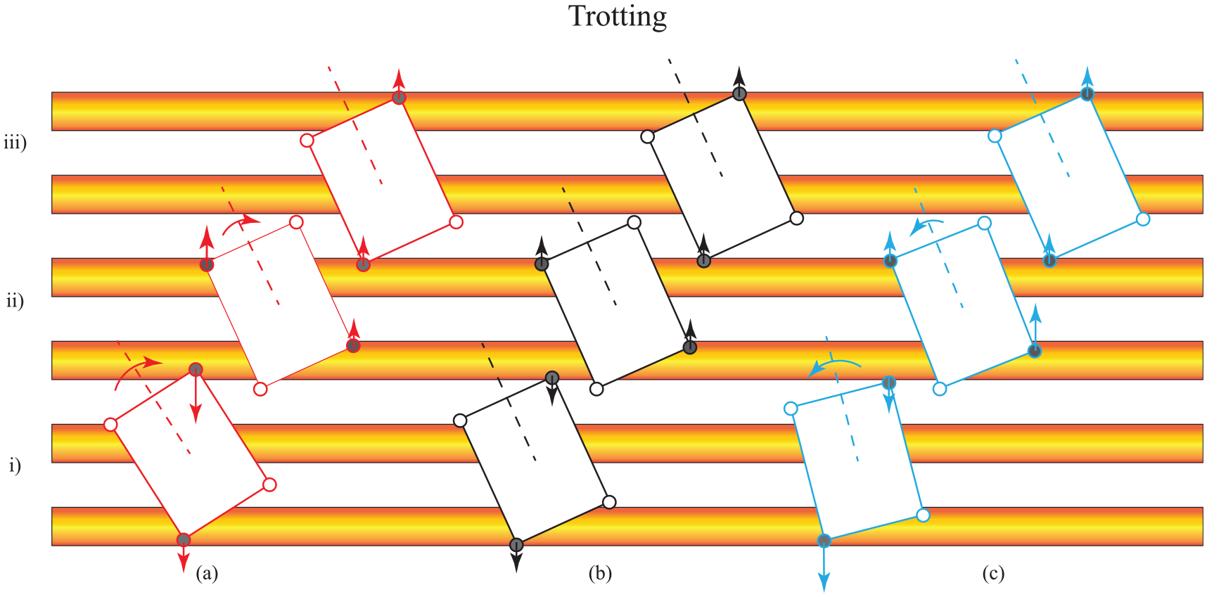
Sequence of images from a trotting experiment showing the robot orientation was locked to
Plots of
3. ODS framework: connectingobstacle-modulated robot CoM dynamicsto leg–obstacle contact positions
The surprisingly simple behavior of the obstacle-modulated robot steady state observed from experiments suggests that despite the complicated, repeated collisions between robot legs and obstacles, there exists a simple mechanism that dominates the obstacle-modulated robot CoM dynamics. In this section, we propose a horizontal plane ODS framework that abstracts and simplifies the complicated low-level contacts and explains the strikingly uniform steady-state robot orientation angles emerging from the leg–obstacle contacts.
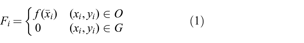
The framework entails three key conceptual components, to generate a simplified representation of the environment, the gait, and the coupling between the two. The first component represents the physical obstacle perturbations as a simplified 2-DoF disturbance force field in the world frame (Section 3.1). The second component interprets the robot gait as an “activation pattern” whereby each activated leg selects the available obstacle disturbances at its location (Section 3.2). Selected disturbances from all activated legs contribute to the total external forces and torques in the third component (Section 3.3), allowing calculation of the obstacle-modulated robot CoM state,
3.1. Obstacle abstraction and disturbance field generation
Qian and Goldman (2015b) found that the orientation of a legged robot could change up to
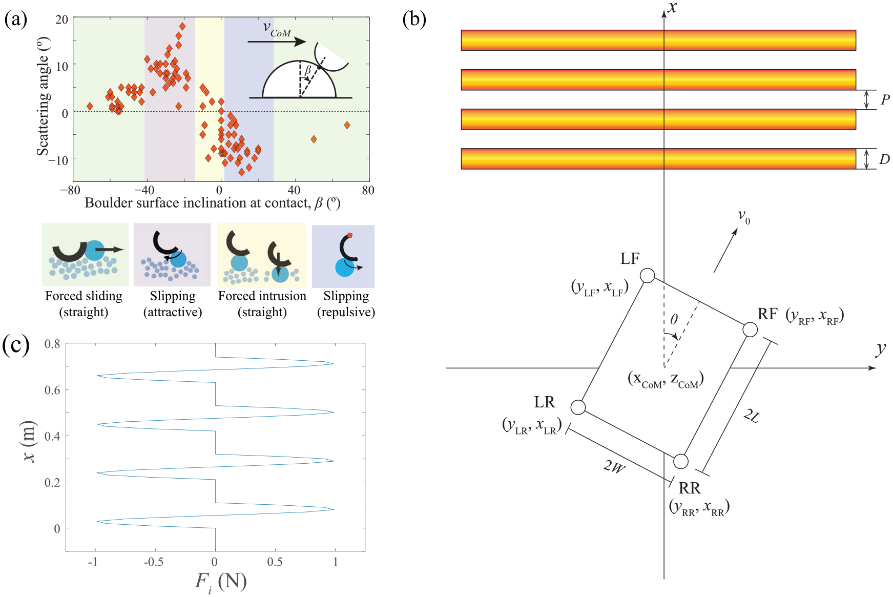
Obstacle disturbance field model. (A) For SLSO interactions, robot orientation change (the “scattering angle”) after the collision depends primarily on the fore–aft inclination angle,
Here we use this dependence to convert physical obstacles into a 1-DoF artificial disturbance force field. In our ODS framework, we model each single-leg, single-obstacle (SLSO) collision as a disturbance force,
The total obstacle disturbance field comes from all obstacles in the physical environment. This 2-DoF ODF field that a robot leg (leg
Here
Since
3.2. Gait pattern abstraction and ODS
The obstacle disturbance force field provides the map of interaction force opportunities. To connect the repeated leg–obstacle collisions to the change of robot state, we represent each robot leg as a “disturbance selector”. At each instant, two conditions are necessary for a leg
The second condition provides a multi-legged robot the option to select different combinations of obstacle disturbances. To study the effect of such selection, we model robot gaits as a time-varying “activation pattern”,
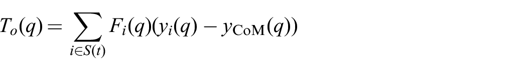
Similarly, the total torque exerted on the robot CoM by the obstacles can be calculated as
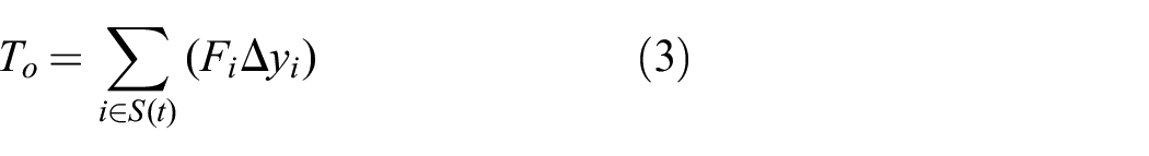
where
We note that the ODS framework presented in this section applies not only to the quadruped demonstrated in Section 4 but also more general multi-legged platforms.
As Equations (2) and (3) stipulate, the obstacle disturbances for multi-leg, multi-obstacle (MLMO) situations depend on both the environment properties (the obstacle disturbance force field) and the choice of gait patterns. Given the same physical environment (i.e., same obstacle disturbance field), the total perturbation to the robot CoM can be significantly different depending on the activated leg groups (i.e., subset of legs) or their sequencing. Therefore, by using a different gait pattern or designing a different leg group sequence (such as a transitional gait), a legged robot can select over a highly diverse range of influences over a fixed terrain (see Section 6).
3.3. Robot CoM dynamics under obstacle disturbance modulation
Combining the disturbance field representation of the leg–environment interaction and the disturbance selection pattern representation of robot gait yields an abstraction of the robot CoM dynamics in response to repeated obstacle collisions.
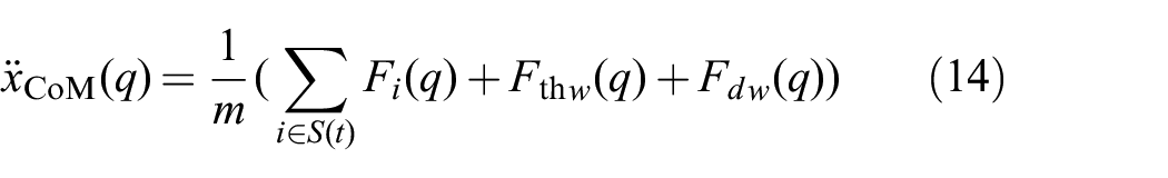
On flat ground, the robot does not experience obstacle disturbances, and the CoM’s fore–aft acceleration is determined by the thrust force,
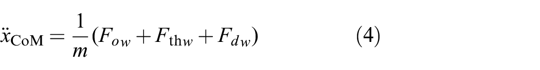
where
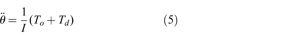
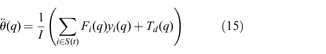
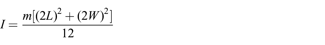
Similarly, our ODS abstraction neglects the small oscillations in orientation due to each step on flat ground while positing an obstacle-engaged disturbance torque,
where
4. Numerical model: capturing robot steady states under periodic obstacle modulation using the ODS framework
In this section, we demonstrate how the obstacle-modulated robot states can be computed using the ODS framework, and we use the results to explain the emergence of the robot’s steady states observed in experiments.
We implemented a numerical model in MATLAB Simulink to compute robot state under repeated obstacle perturbation. To facilitate comparison with experiments, in the numerical study we used the same setup as the experiment, with a quadrupedal robot traversing over evenly spaced cylindrical obstacles, and we compared the behaviors of the bounding and trotting gaits. All dimensions used in the simulation were directly measured from the experiments.
The numerical model executes three steps corresponding to the three components in the ODS framework. The first step (Section 4.1) computes the disturbance force field in the world frame based on the distribution of the obstacles in the physical environment. The second step (Section 4.2) generates a time series of leg activation set based on the two given gait patterns (Equations (12) and (13)), and computes the total disturbance force and torque exerted on the robot CoM. The third step (Section 4.3) updates the time-varying robot CoM state (fore–aft position
In Section 4.4, we show that the highly simplified horizontal-plane model is able to successfully capture the equilibrium steady-state behaviors of the coupled robot–obstacle system observed from experiments for both bounding and trotting gaits. In addition, the framework allows examination of forces and torques exerted on robot legs and CoM that lead to the observed steady states, and therefore facilitates discovery of the underlying mechanism of obstacle modulation behind seemingly complicated repeated leg–obstacle collisions.
4.1. Obstacle abstraction
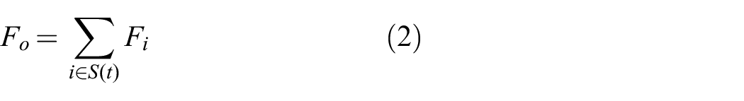
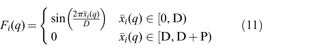
Based on the ODS framework, each obstacle is modeled as a localized disturbance field, where the direction and magnitude of the disturbance force at each fore–aft position depends on the obstacle surface inclination. For the cylindrical obstacles (logs) used in our experiment, the SLSO disturbance
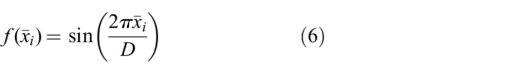
This function qualitatively captures the dependence of obstacle disturbance observed in Qian and Goldman (2015b), where leg contacting on positive (
As mentioned previously,
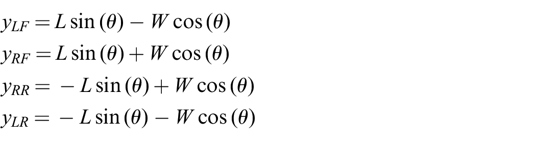
The fore–aft position of leg


In the experiments, obstacles were an array of evenly spaced logs along the
Here
4.2. Disturbance selection
In a bounding gait, the two front legs always “activate” together to engage the obstacle disturbances at the same time, and then alternate with the two rear legs every half stride period,
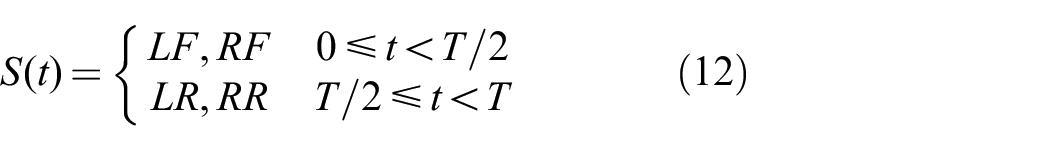
We note that our model is highly simplified and not intended to take into account all physical details. In this highly simplified model, we assume perfectly alternating pairs. In physical experiments, the two pairs can overlap during stance depending on the duty cycle. Despite such simplification we show in Section 4.4 that the steady states persist.
Similarly, in a trotting gait, two diagonal legs always “activate” together and alternate with the other pair every half gait period. The activation set
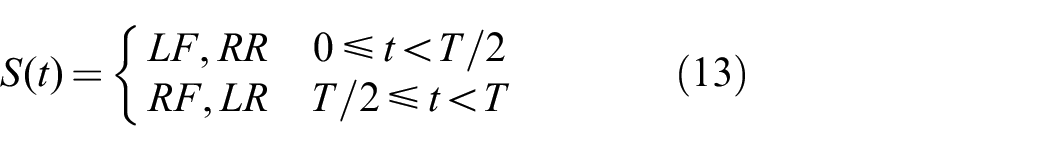
where
With Equations (12) and (13), we can calculate the total obstacle disturbance force and torque on robot CoM using Equations (2) and (3):
In this study, owing to the symmetry of the obstacles in the horizontal direction, the lateral position of the CoM was not updated.
6
Here
Representing gaits as disturbance selection patterns allows a simplified analysis of how different
4.3. State prediction
Here we compute the robot dynamics for different obstacle distributions and gait patterns using the total disturbance force and torque computed in the disturbance selection step (Section 4.2).
The fore–aft acceleration of the robot CoM in the world frame was calculated using the equation of motion (4). As mentioned in Section 3.3, on flat ground the robot’s fore–aft acceleration is determined by the thrust force,

where
The fore–aft position of the robot in the world frame,
In our simulation,
Similarly, the orientation of the robot,

was implemented to stabilize the robot after the perturbation:
In our experiments, the weight of the robot, was primarily due to the battery (
Here
4.4. Capturing the observed steady states with the highly simplified ODS model
Here we calculate the robot steady-state orientation states for bounding and trotting using the numerical model. We compute robot state
Figure 7A and B show the robot orientation state computed from stabilized trials. Figure 7A demonstrates that similar to experiment observations, despite variations in initial conditions, a bounding robot has a steady-state orientation at
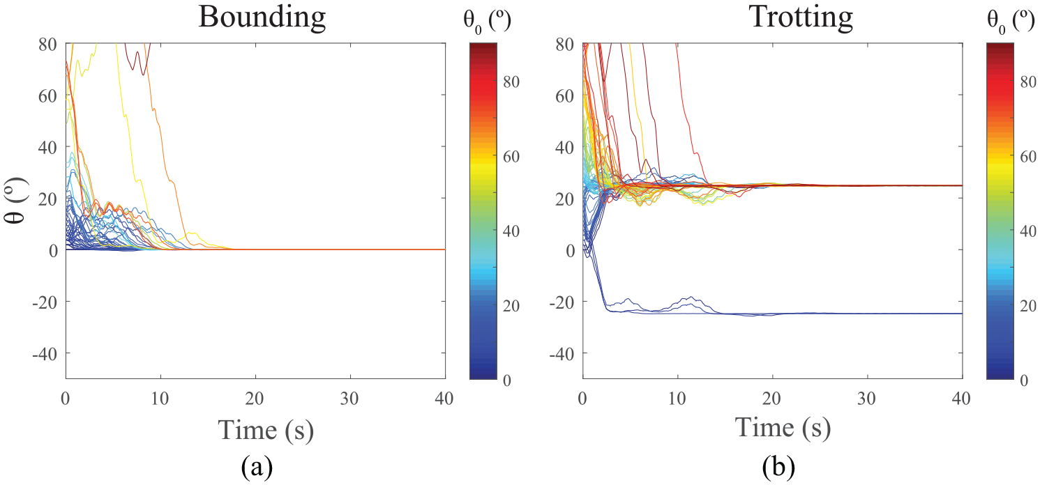
ODS framework-based numerical simulation of robot orientation angle under repeated obstacle modulation (Equations (14) and (15)). Since limit cycles are beyond the scope of this article, only equilibrium trajectories with non-
5. Steady-state mechanism and predictionof equilibrium orientations using the ODS framework
The ODS framework not only allows numerically capturing the coupled dynamics, but since the computation of the change of states arises from physical understanding of low-level leg–obstacle interactions, the framework also allows close examination of the forces and torques that lead to the steady states, and reveals the underlying mechanism that produces or maintains the equilibria of the coupled system.
In this section, we first discuss the mechanism for the emergence of the steady-state robot orientations observed in both simulation and experiments using the ODS framework (Section 5.1). We then use this discovered mechanism to develop a theoretical model (Section 5.2) to analytically calculate stable equilibrium states of robot orientation for different environments, robot morphology and gait parameters without requiring numerical simulation.
5.1. Mechanism of obstacle-modulated steady state
Here we calculate the equilibrium positions of the robot orientation using the ODS framework. The orientation state of the robot is
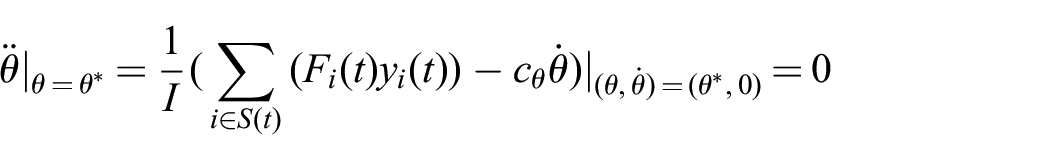
which leads to the following condition at
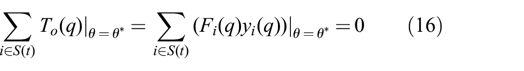
Intuitively, this means that the sum of torques from all contacting legs
5.1.1. Bounding analysis
For the bounding gait, the set of contacting legs
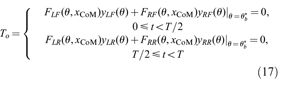
A sufficient condition for
As discussed in Section 4.1, the ODF in the world frame for any contacting leg,
Therefore, if there exists a
Obviously, another sufficient condition that satisfies Equation (17) would be
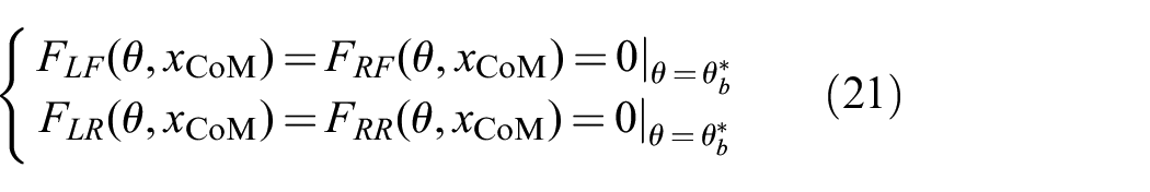
This condition corresponds to the trivial
5.1.2. Trotting analysis
For the trotting gait, the set of contacting legs
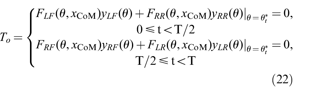
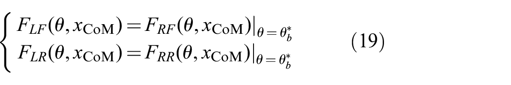
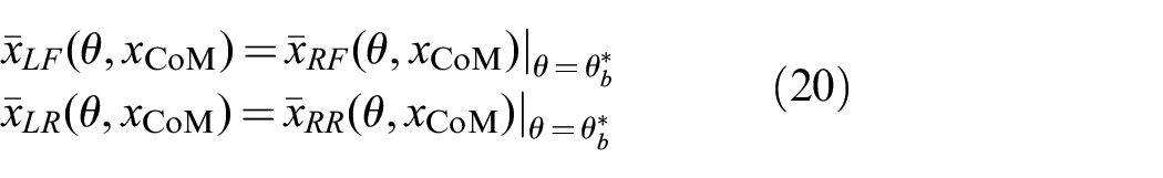
A sufficient condition for
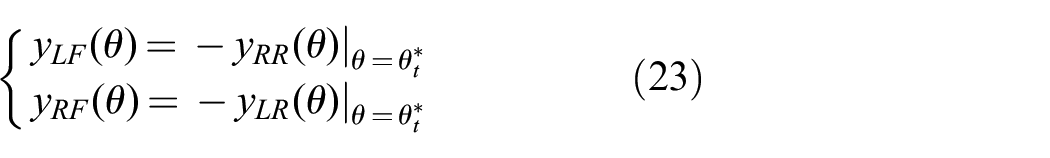
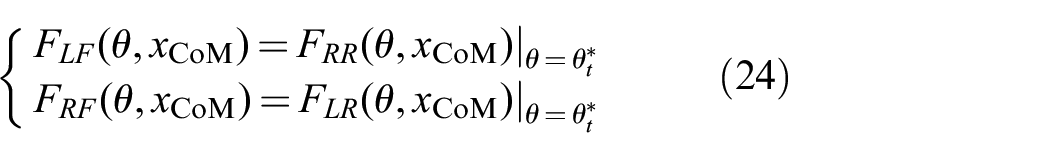
and therefore cancel out the total torque on the CoM.
Using Equation (1) we can further simplify Equation (24) to the following:
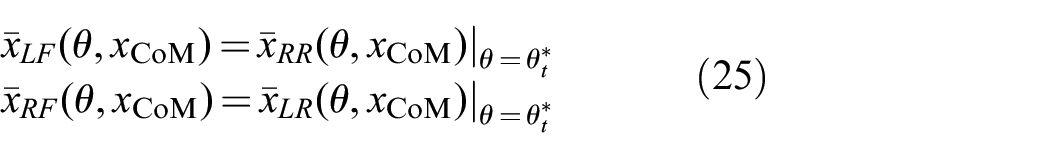
In Section 5.2 we demonstrate how to use this criterion to calculate the equilibrium orientation of trotting gait,
Similar to the bounding analysis, another sufficient condition that satisfies Equation (22) would be
which corresponds to the trivial
5.2. Analytically calculating equilibrium orientations based on the steady-state mechanism
The derived equilibrium criteria (Equation (20) for bound, and Equation (25) for trot) in Section 5.1 provide a sufficient condition to maintain a steady-state orientation under repeated obstacle perturbation, which is to let the synchronously activated two legs always select the opposite obstacle disturbance torques. In this section, we show that this condition allows us to theoretically predict steady-state orientation positions observed from our experiments (Section 2) and simulation (Section 4.3) without numerical simulations.
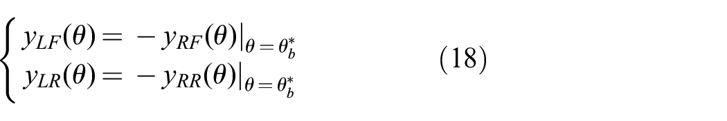
In our experimental setup, the obstacle spatial distribution is periodic, and therefore the robot did not need to actively adapt its gait pattern to select the same
These two equations provide the constraining conditions to calculate equilibrium orientation angles for periodic gaits like bounding and trotting. We interpret such constraints as solving a “spatial period matching” constraint.
The spatial period of a periodic robot gait,

For the bounding gait, there are two pairs of synchronized legs,

Similarly, for the trotting gait, the two spatial periods can be calculated as the

At
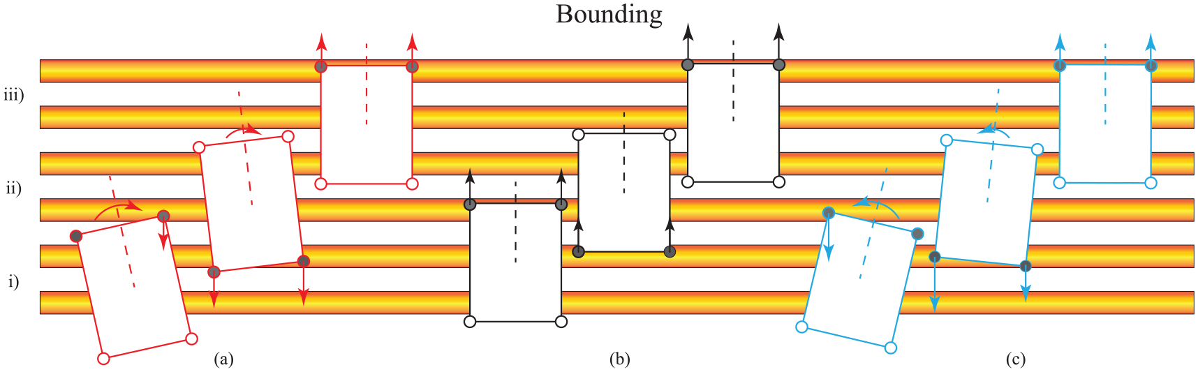
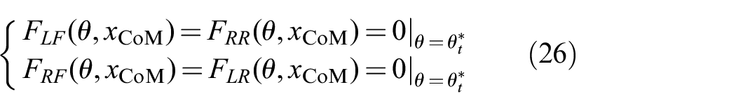
Mechanism for a bounding robot to stabilize at
Mechanism for a trotting robot to stabilize at
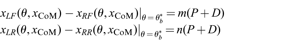
Therefore, the equilibrium orientation can be calculated by solving the spatial period matching constraints, which can be written for bounding as

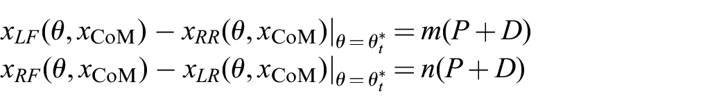
and for trotting as
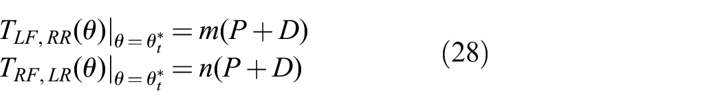
The leg–obstacle contact positions observed from both experiments (Figures 4 and 5, Extensions 1 and 2) and numerical simulation (Figure 10, Extensions 3 and 4) are qualitatively consistent with the criteria described by Equations (27) and (28).
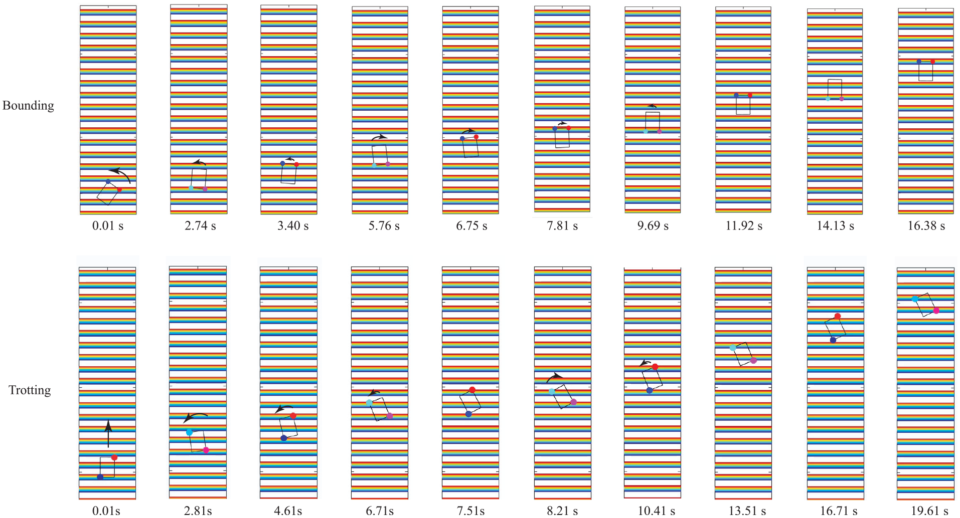
Sequence of images from simulation showing a bounding robot’s orientation locked to
The spatial period matching criterion enabled theoretical prediction of obstacle-modulated robot equilibrium states, and predictions of the dependence of the equilibrium angles on robot and environment parameters. Figure 11 shows the analytical prediction of equilibrium orientations for different obstacle spacings and robot aspect ratios. The model prediction agrees well with numerical simulation results and measurements from experiments.
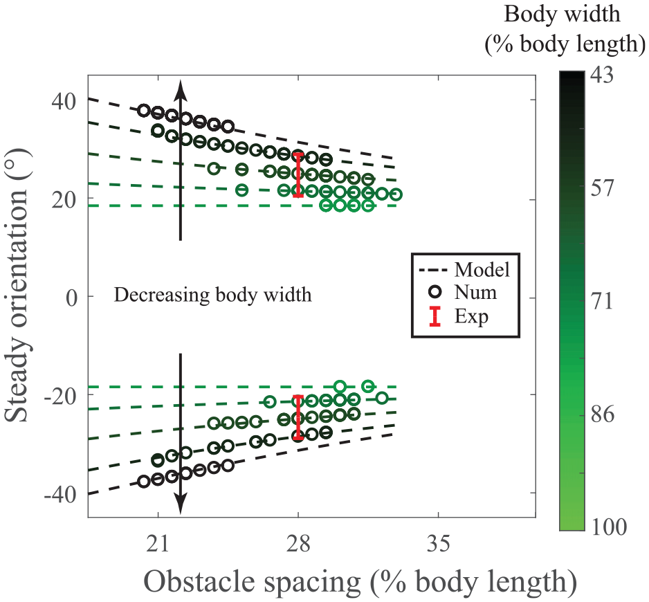
Prediction of trotting robot equilibrium orientation angles as a function of log spacing for different robot aspect ratios. Red error bars represent average final orientation angles measured from trotting experiments (Figure 3C and D) with a robot body width of
Going forward, this stabilizing mechanism begins to suggest a novel gait control method to stabilize robot orientation under repeated obstacle collisions and disturbances. In Section 6, we discuss how multi-legged robots can use the ODS framework to actively adjust gait sequence to robustly move through randomly cluttered environments.
6. Broader applicability of the ODS framework
Section 5 reveals that the mechanism of the equilibrium robot orientation under repeated obstacle collisions is due to synchronized robot legs selecting cancelling obstacle disturbances and therefore neutralizing the total perturbation experienced by the CoM. For the structured environment studied in this article, periodic robot gaits passively generate such disturbance cancellation at the equilibrium orientations.
For non-structured environments, periodic gaits will no longer lead to equilibrium orientations. However, with the ODS representation (Section 3.1), a robot can plan a non-periodic gait to actively select cancelling obstacle disturbance torques and to reduce the perturbation in its orientation. Similarly, a robot might plan its gait to actively regulate total obstacle disturbance forces to maintain a constant speed.
In addition to stabilization, a robot can also use the ODS framework to actively exploit obstacle disturbances to achieve faster speed in translation or rotation. For example, to obtain a boost in the speed at each step, a robot might adjust the timing or position of obstacle interaction to always engage the obstacle on the negative (i.e., downhill) slopes. To exploit obstacles to turn clockwise, a robot can simply have all the right-hand side legs begin stance phase on positive (i.e., uphill) obstacle slopes and all the left-hand side legs begin stance phase on negative (i.e., downhill) slopes. Future work will investigate sensing options to implement these applications.
7. Conclusion
In this article, we propose a novel ODS framework that allows investigating and predicting robot dynamics under repeated obstacle disturbances. The ODS framework provides a novel representation of both physical environments and robot gait patterns, which allows systematic analysis of complex interactions between multi-legged platforms and obstacles, and suggests an approach to formal reasoning about how a locomotor could use the gait space affordances to actively exploit disturbances and collisions.
The ODS framework represents the cluttered environments as sources of obstacle disturbance force fields. This representation significantly simplifies the complexity of the contacts between high-DoF robot legs and high-DoF physical obstacles, and for the first time allow the assessment of opportunities for a robot to exploit its interaction with the environment as a source of locomotion affordances (Gibson, 1979) derived from locally-sensible physical properties such as shape and size.
The ODS framework represents robot legs or body segments as a collection of “disturbance force selectors” leveraged to adjust actual total environment perturbation that affects CoM dynamics. With sufficient knowledge of the environment, we envision that a multi-legged robot can use the ODF framework to adjust the timing or contact position of leg–obstacle interactions to actively select available disturbances and generate desired interaction dynamics for an “obstacle-aided” locomotion and navigation in cluttered environments.
We note that this study is the first step towards a more complete connection between gait space and environment affordances. Future work such as extension of the horizontal-plane model to three dimensions, and further investigation of coupling between non-periodic gaits with less-structured environments, will allow creation of more general and complete versions of the disturbance selection framework. We envision such development will aid control and planning strategies for future robots to move through complex environments.
Footnotes
Appendix A. Index to multimedia extensions
Archives of IJRR multimedia extensions published prior to 2014 can be found at http://www.ijrr.org, after 2014 all videos are available on the IJRR YouTube channel at http://www.youtube.com/user/ijrrmultimedia
Experimental bounding gait
Experimental trotting gait
Simulation bounding gait
Simulation trotting gait
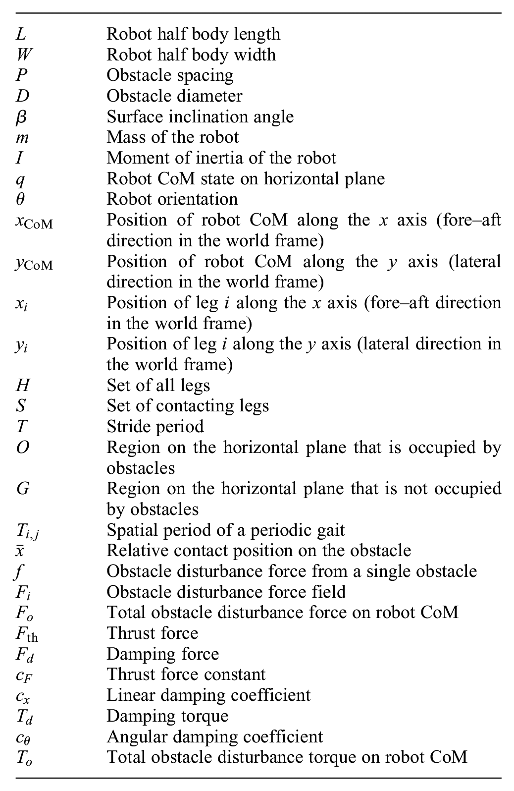
Appendix B. List of symbols
| Robot half body length | |
| Robot half body width | |
| Obstacle spacing | |
| Obstacle diameter | |
| Surface inclination angle | |
| Mass of the robot | |
| Moment of inertia of the robot | |
| Robot CoM state on horizontal plane | |
| Robot orientation | |
| Position of robot CoM along the axis (fore–aft direction in the world frame) | |
| Position of robot CoM along the axis (lateral direction in the world frame) | |
| Position of leg along the axis (fore–aft direction in the world frame) | |
| Position of leg along the axis (lateral direction in the world frame) | |
| Set of all legs | |
| Set of contacting legs | |
| Stride period | |
| Region on the horizontal plane that is occupied by obstacles | |
| Region on the horizontal plane that is not occupied by obstacles | |
| Spatial period of a periodic gait | |
| Relative contact position on the obstacle | |
| Obstacle disturbance force from a single obstacle | |
| Obstacle disturbance force field | |
| Total obstacle disturbance force on robot CoM | |
| Thrust force | |
| Damping force | |
| Thrust force constant | |
| Linear damping coefficient | |
| Damping torque | |
| Angular damping coefficient | |
| Total obstacle disturbance torque on robot CoM |
Acknowledgements
We thank Christopher Zawacki for his assistance in designing the robot platform. We thank Zhichao Liu and Divya Ramesh for their assistance in preliminary data collection.
Funding
The author(s) disclosed receipt of the following financial support for the research, authorship, and/or publication of this article: This research was supported by the National Science Foundation (NSF) under an INSPIRE award (number CISE NRI 1514882) and NRI INT award (number 1734355).