
Abstract
In this work, we propose algorithms to explicitly construct a conservative estimate of the configuration spaces of rigid objects in two and three dimensions. Our approach is able to detect compact path components and narrow passages in configuration space which are important for applications in robotic manipulation and path planning. Moreover, as we demonstrate, they are also applicable to identification of molecular cages in chemistry. Our algorithms are based on a decomposition of the resulting three- and six-dimensional configuration spaces into slices corresponding to a finite sample of fixed orientations in configuration space. We utilize dual diagrams of unions of balls and uniform grids of orientations to approximate the configuration space. Furthermore, we carry out experiments to evaluate the computational efficiency on a set of objects with different geometric features thus demonstrating that our approach is applicable to different object shapes. We investigate the performance of our algorithm by computing increasingly fine-grained approximations of the object’s configuration space. A multithreaded implementation of our approach is shown to result in significant speed improvements.
1. Introduction
A basic question one may ask about a rigid object is to what extent it can be moved relative to other rigidly fixed objects in the environment. In robotic manipulation, this has lead to the notion of a cage. An object is considered caged by rigid fixtures, or a robotic manipulator, if it cannot be moved arbitrarily far from its initial configuration. In terms of the configuration space of the rigid object, this is equivalent to being able to answer whether an object is located in a configuration contained in a bounded path component of its configuration space. Similarly, in fields such as chemistry and biology, this notion of a cage is a useful basic concept for predicting how molecules can restrict each other’s mobility which has important applications in drug delivery and related problems (Mitra et al., 2013; Rother et al., 2016).
The main challenge in caging verification is that the configuration space of a rigid object in three dimensions is, in general, a 6D subset of
We study caging as a special case of proving path non-existence between a pair of configurations. To show that two configurations are disconnected, we construct an approximation of the object’s collision space. Intuitively, we construct a set of slices of the object’s collision space corresponding to subspaces of fixed orientations of the object, see Figure 1. We then compute the free space approximation as the complement to the collision space of each slice. By construction, our collision space approximation is a proper subset of the real collision space, which implies that when our algorithm reports that the two configurations are not path-connected, then there is no path between them in the real free space. However, for the same reason, our algorithm is not guaranteed to find all possible caging configurations, since we do not reconstruct the entire collision space.
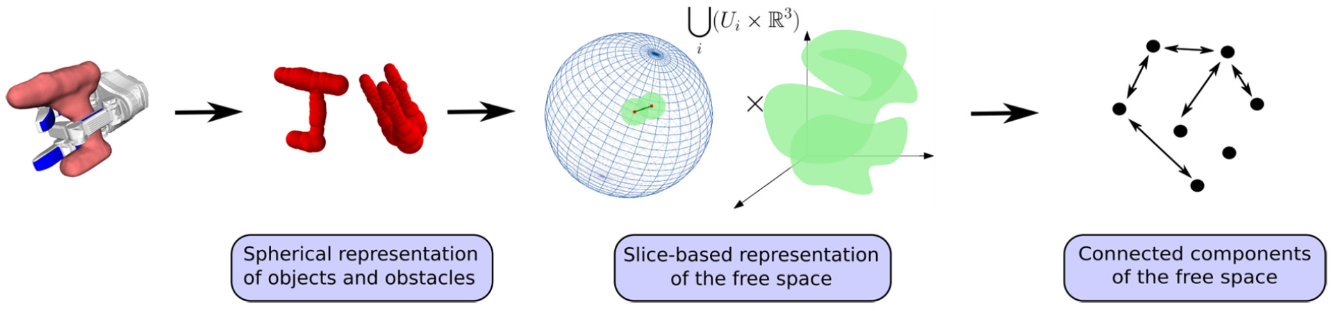
Diagram of our method. We approximate the collision space of an object by choosing a finite set of fixed object’s orientations and considering the corresponding slices of the collision space to
The key contribution of the work we present here is to show that it is possible to compute explicit approximations of configuration spaces of generic rigid bodies in three dimensions relatively efficiently, while maintaining provability guarantees with respect to reasoning about caging and, more generally, path existence. Our technique for constructing such an approximation is based on the following key insights.
The presented work constitutes an extended version of our initial work at WAFR’18 (Varava et al., 2018). It features a revised introduction and algorithms description, as well as extended experimental results, a parallelized version of the presented algorithm and its evaluation on 3D models of real objects.
2. Related work
In manipulation, caging can be considered as an alternative to a force-closure grasp (Makita and Maeda, 2008; Makita et al., 2013; Pokorny et al., 2013; Varava et al., 2016), as well as an intermediate step on the way towards a form-closure grasp (Rodriguez et al., 2012). Unlike classical grasping, caging can be formulated as a purely geometric problem, and therefore one can derive sufficient conditions for an object to be caged. To prove that a rigid object is caged, it is enough to prove this for any subset (part) of the object. This allows one to consider caging a subset of the object instead of the whole object, and makes caging robust to noise and uncertainties arising from shape reconstruction and position detection.
The notion of a planar cage was initially introduced by Kuperberg (1990) as a set of
In the above-mentioned works, fingertips are represented as points or spheres. Later, more complex shapes of caging tools were taken into account by Pokorny et al. (2013), Stork et al. (2013), Varava et al. (2016), and Makita and Maeda (2008); Makita et al. (2013). In these works, sufficient conditions for caging were derived for objects with particular shape features. Makapunyo et al. (2013) proposed a heuristic metric for partial caging based on the length and curvature of escape paths generated by a motion planner. The authors suggested that configurations that allow only rare escape motions may be used as cages in practice.
We address caging as a special case of the path non-existence problem: an object is caged if there is no path leading it to an unbounded path-connected component. The problem of proving path non-existence has been addressed by Basch et al. (2001) in the context of motion planning, motivated by the fact that most modern sampling-based planning algorithms do not guarantee that two configurations are disconnected, and rely on stopping heuristics in such situations (Latombe, 1991). Basch et al. (2001) provided an algorithm to prove that two configurations are disconnected when the object is “too big” or “too long” to pass through a “gate” between them. There are also some related results on approximating configuration spaces of 2D objects. Zhang et al. (2008) used approximate cell decomposition and prove path non-existence for 2D rigid objects. They decompose a configuration space into a set of cells and for each cell decide if it lies in the collision space. McCarthy et al. (2012) proposed a related approach. There, they randomly sampled the configuration space of a planar rigid object and reconstructed its approximation as an alpha complex. They later used it to check the connectivity between pairs of configurations. This approach has been later extended to planar energy-bounded caging by Mahler et al. (2016).
The problem of explicit construction (either exact or approximate) of configuration spaces has been studied for several decades in the context of motion planning, and a summary of early results can be found in the survey by Wise and Bowyer (2000). Lozano-Perez (1983) introduced the idea of slicing along the rotational axis. To connect two consecutive slices, the authors proposed to use the area swept by the robot rotating between two consecutive orientation values. Zhu and Latombe (1991) extended this idea and used both outer and inner swept areas to construct a subset and a superset of the collision space of polygonal robots. The outer and inner swept areas are represented as generalized polygons defined as the union and intersection of all polygons representing robot’s shape rotating in a certain interval of orientation values, respectively. Several recent works propose methods for exact computation of configuration spaces of planar objects (Behar and Lien, 2013; Milenkovic et al., 2013). Behar and Lien (2013) proposed a method towards exact computation of the boundary of the collision space. Milenkovic et al. (2013) explicitly compute the free space for complete motion planning.
Thus, several approaches to representing configuration spaces of 2D objects, both exact and approximate, have been proposed and successfully implemented in the past. The problem is however more difficult if we consider a 3D object, as its configuration space is 6D. In the recent survey on caging by Makita and Wan (2017), the authors hypothesized that recovering a 6D configuration space and understanding caged subspaces is computationally infeasible. To the best of the authors’ knowledge, we present the first practical and provably correct method to approximate a 6D configuration space.
Our approximation is computed by decomposing the configuration space into a finite set of lower-dimensional slices. Although the idea of slicing is not novel and was introduced by Lozano-Perez (1983), recent advances in computational geometry and topology, as well as a significant increase in processing power, have made it possible to approximate a 6D configuration space on a common laptop. We identify two main challenges to slicing a 6D configuration space of a rigid object: how to quickly compute 3D slices of the free space, and how to efficiently discretize the orientation space. For slice approximation, our method relies on the fact that the collision space associated to a rigid object with a fixed orientation and an obstacle represented as a union of balls is itself a union of balls. Then we use the dual diagram to a union of balls presented by Edelsbrunner (1999) as an approximation of the free space of the slice. In this way, we do not need to use generalized polygons, which makes previous approaches more difficult in two dimensions and very hard to generalize to 3D workspaces. To discretize
Finally, our method does not require precise information about the shape of objects and obstacles, and the only requirement is that balls must be located strictly inside them, which makes our approach more robust to noisy and incomplete sensor data.
We implemented our algorithm to approximate 3D and 6D configuration spaces and verify that it has in practice a reasonable runtime on a single core of Intel Core i7 processor. We provide a parallel implementation which makes use of modern parallel CPU architectures and investigate the effect of parallelization on the runtime of the algorithm.
3. Definitions and notation
3.1. Objects and obstacles
For the sake of generality, in this article we use the terms “object” for objects and autonomous rigid robots (e.g., disk robots) moving in
When formally defining an object and a set of obstacles, we make a few mild assumptions to define a large class of shapes and include most of the regular objects in the real world. Since we want to represent both the object and the obstacles as a set of
In the above definition, the interior of
We approximate both the obstacles,
Let
Note that this definition allows the object to be in contact with the obstacles.
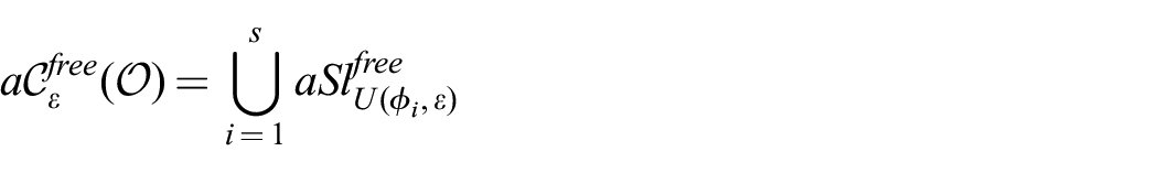
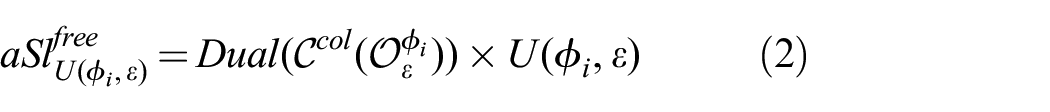
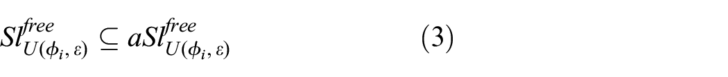
To compute path-connected components of the free space, we decompose the free space into a set of
3.2. Slice-based representation of the configuration space
In our previous work (Varava et al., 2017), we suggested that configuration space decomposition may be a more computationally efficient alternative to its direct construction. We represent the configuration space of an object as a product
We denote a slice of the collision (free) space by
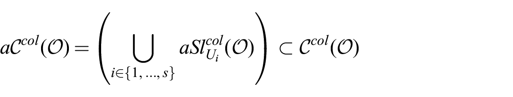
In this way, we approximate the entire collision space by a subset
Now, we discuss how to construct slice approximations.
3.3. An
-core of the object
First observe that by Definition 3, if a subset
Therefore, if some subset
Now, for an object
In Varava et al. (2017), we showed that for an object
An
In Section 5, we address the problem of representing and discretizing the space of orientations
4. Existence of
-clearance paths
For safety reasons, in path planning applications a path is often required to keep some minimum amount of clearance to obstacles. The notion of clearance of an escaping path can also be applied to caging: one can say that an object is partially caged if there exist escaping paths, but their clearance is small and therefore the object is unlikely to escape.
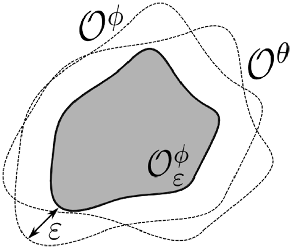
Consider a superset of our object
Consider now the following modification of our algorithm. If we enlarge the
One application of this observation is narrow passage detection. One can use our free space approximation to identify narrow passages as follows. If two configurations are disconnected in
Furthermore, we can view
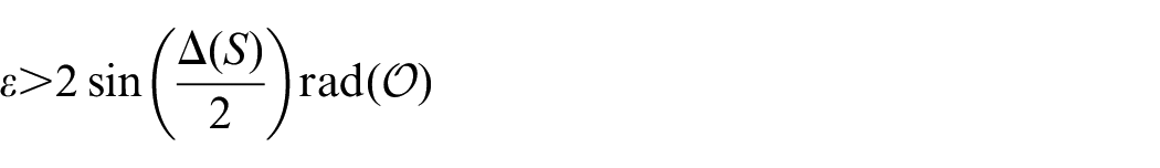
This leads us to a tradeoff between the desired accuracy of our approximation expressed in terms of clearance
5. Discretization of
Elements of
Our goal now is to derive upper bounds for maximum displacement of any point in the object to make sure that the
5.1. Displacement in two dimensions
In our previous work (Varava et al., 2017), we derived the following upper bound for the displacement of a 2D object:

assuming that we rotate the object around its geometric center,
In the 2D case, discretization of the rotation space is simple: given a desired number of slices, we obtain the displacement
5.2. Displacement in three dimensions
We now discuss the 3D case. Similarly to the previous case, our goal is to cover
A unit quaternion
We use the angular distance (Yershova et al., 2009) to define the distance between two orientations:

where
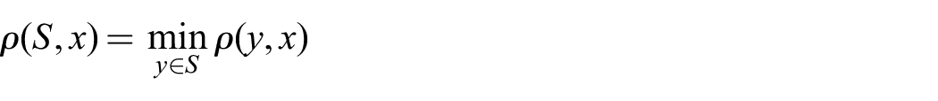
Yershova et al. (2009) provided a deterministic sampling scheme to minimize the dispersion
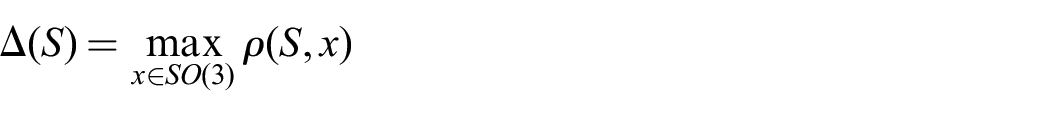
Intuitively, the dispersion of a set
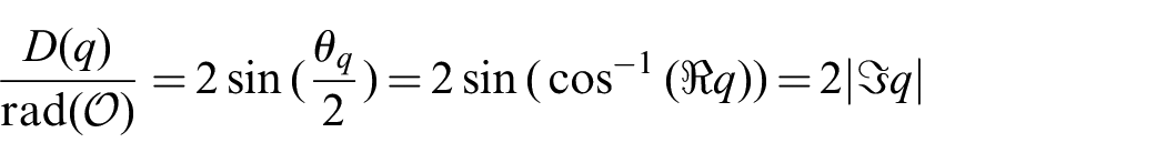
Now, Proposition 1 allows us to establish the relation between the distance between two quaternions and displacement associated to the rotation between them.

The proof of Proposition 1 can be found in the appendix.
This means that if we want to cover
Given such a cover of
To compute the graph adjacency, we note that if two slices
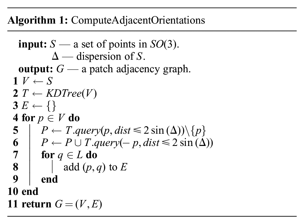
The algorithm starts by setting
5.3. Different resolutions and dispersion estimation
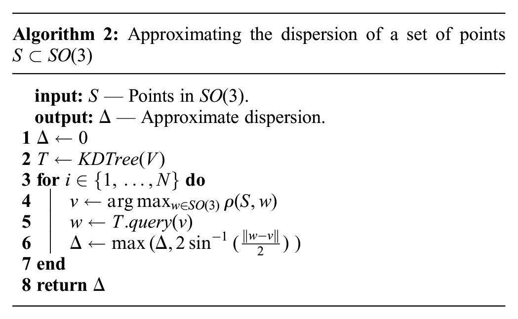
One of the prerequisites of Algorithm 1 is the availability of an estimate of the dispersion of
However, since this is an upper bound, and we want a tighter estimate of the dispersion to reduce the number of slices, in our implementation we employed a random sampling method to estimate the dispersion.
Algorithm 2 summarizes the procedure by which we approximate the dispersion. On each iteration of the main loop (lines 3-6) it retrieves an element of
5.4. The choice of
and
discretization in practice
Depending on the chosen discretization of the orientation space and its dispersion, the
To discretize
Dispersion of the grids used to discretize
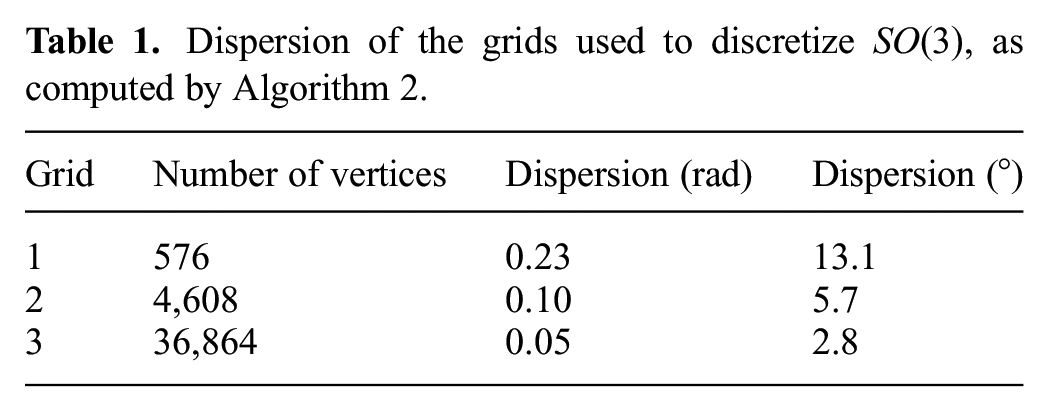
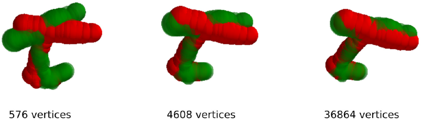
Figure 3 illustrates how much an object rotates between two neighboring orientations in each of these grids. In our experiments, we analyze how the performance of the algorithm is affected by the choice of a grid.
Approximation of a drill as a collection of balls around its medial axis. This representation is visualized at two distinct orientations which are adjacent in the graph over
6. Free space approximation
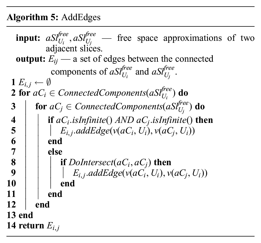
Let us now discuss how we connect the slices to construct an approximation of the entire free space, see Algorithm 3.
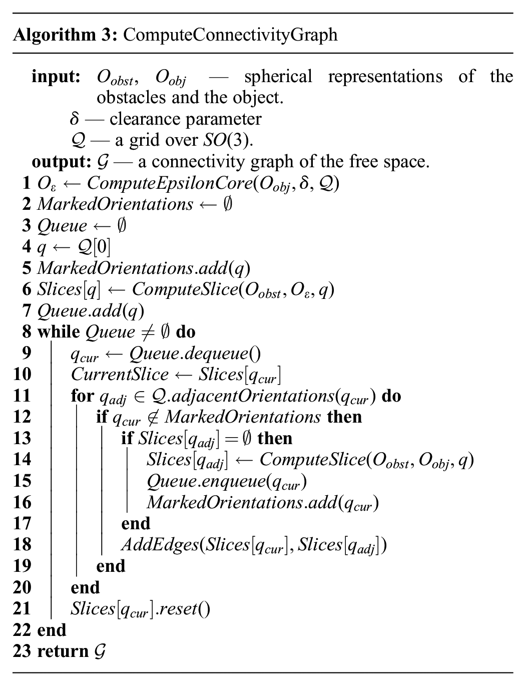
Let
We start by choosing one orientation and run a breadth-first search (BFS) over the orientation grid
In order to query connectivity, the slices approximations should be preserved. In our current implementation, each slice is deleted as soon as the connectivity check between it and the slices adjacent to it is performed, in order to optimize memory usage. In this case, one can save the slice approximation together with the resulting graph to disk, for later use by a querying algorithm.
6.1. Construction of slices
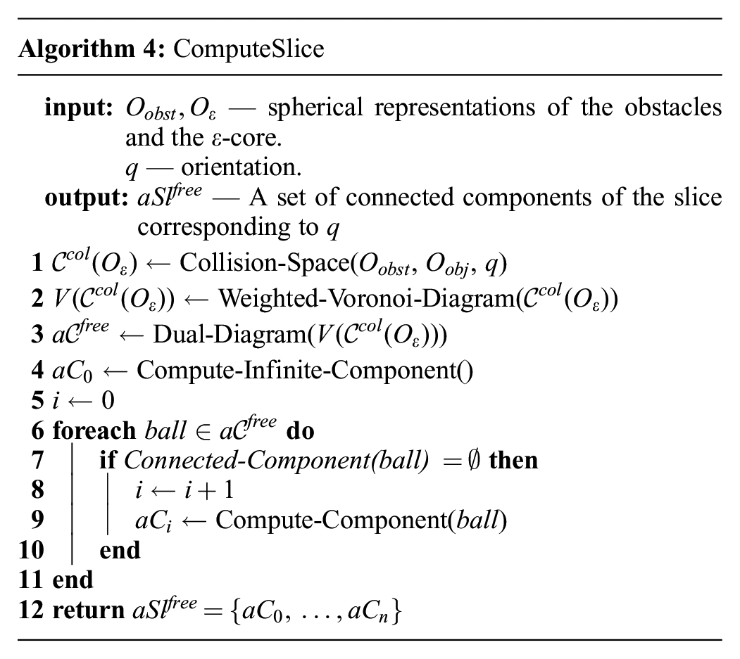
Now, let us discuss how we approximate path-connected components of the free space of each slice, see Algorithm 4. Given a set of obstacles, an object, and a particular orientation of its
In Varava et al. (2017), we derived the following representation for the collision space of
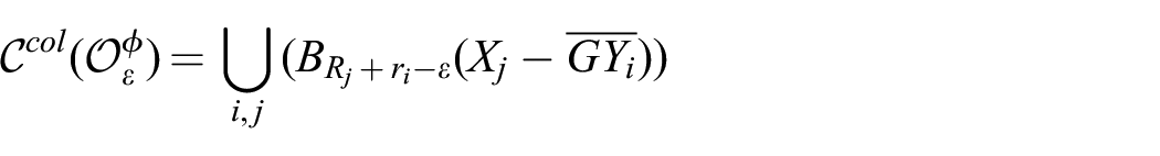
where
Indeed, the object represented as a union of balls collides with the obstacles if at least one of the balls is in collision, so the collision space of the object is a union of the collision spaces of the balls shifted with respect to the position of the balls centers:
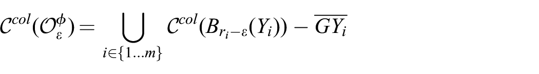
Now, each ball collides with the obstacles when the distance from the obstacles to its center is not greater than the radius of the ball, so the collision space of a single ball of radius
At the next step, we approximate the free space of the slice. For this, we approximate the complement of the collision space by constructing the dual diagram (Edelsbrunner, 1999) to the set of balls representing the collision space.
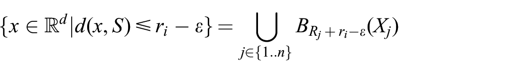
A dual diagram
A weighted Voronoi diagram is a special case of a Voronoi diagram, where instead of Euclidean distance between points, a special distance function is used (Voronoi, 1907). In our case, the weighted distance of a point
To construct a dual diagram of a union of balls
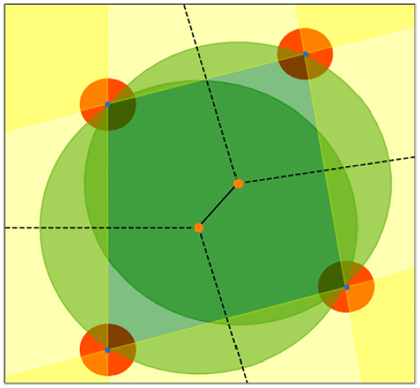
Green circles and yellow halfspaces (“infinite circles”) together represent a dual diagram of the red circles. Green circles are centered at the vertices of the Voronoi diagram; yellow halfspaces correspond to infinite edges of the diagram (dashed lines).
From left to right, the elements of the dual diagram approximating the free space. We start with building a Voronoi diagram (visualized in black); the second figure shows a set of finite orthogonal balls, corresponding to the regular edges of the diagram; the third figure visualizes the “infinite” orthogonal balls corresponding to the infinite edges of the diagram; finally, the last figure depicts full diagram. Red circles with blue centers represent the collision space, the yellow circles approximate the dual diagram.
After constructing the dual diagram, we find pairs of overlapping balls in it and run depth-first search to identify connected components. It is important to note that each dual diagram always has exactly one unbounded connected component, representing the outside world.
Finally, let us discuss how to understand whether free space approximations of neighboring slices overlap. In Algorithm 5, to check whether two connected components in adjacent slices intersect (line 8), we recall that they are just finite unions of balls. Instead of computing all pairwise intersections of balls, we approximate each ball by its bounding box and then use the CGAL implementation of Zomorodian’s algorithm (Zomorodian and Edelsbrunner, 2000), which efficiently computes the intersection of two sequences of three-dimensional boxes. Every time it finds an overlapping pair of boxes, we check whether the respective balls also intersect.
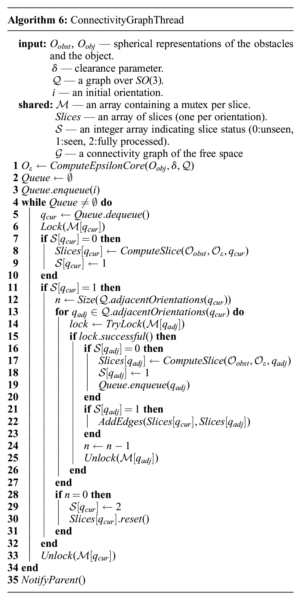
7. Parallel implementation
To increase the performance of our algorithm, we designed and implemented a parallelized version that uses multiple threads to compute different slices simultaneously. Algorithm 6 describes the process.
Recall that in the single-thread version of the algorithm (see Algorithm 3), we performed BFS over the orientation grid
A nave approach to parallelization would have a main thread call child threads on to process each new orientation in the queue, however since the orientations are enqueued in sequence it would increase the chances that different threads try to compete for computing the same slice data, necessitating threads to wait for each other to finish. Instead we opted for a simple scheme where each thread performs its own BFS from a different point in the tree taking care to lock access to resources every time shared data is accessed.
Algorithm 6 describes the procedure followed by each thread. It assumes that all threads share an access to the array of slices and the connectivity graph, as well as the book-keeping data, i.e., an array of mutexes, and an array containing the status of each slice. The status array (
The main loop (lines 4–33) proceeds as follows: it pops the first element of the queue
This procedure guarantees the absence of data corruption since in order to change the data associated to slices or the edges between them, the corresponding mutexes need to be locked first. Furthermore the algorithm is guaranteed to be lock-free given that:
if two threads try to lock the same
if there is an edge
Note also that each thread is guaranteed to terminate since orientations only get enqueued if their status is unseen (
Algorithm 6 is called by a threadpool as shown in Algorithm 7. The algorithm ComputeConnectivityGraphParallel works by setting up the data that must be shared between the several instances of ConnectivityGraphThread, and calling it starting from different orientations in
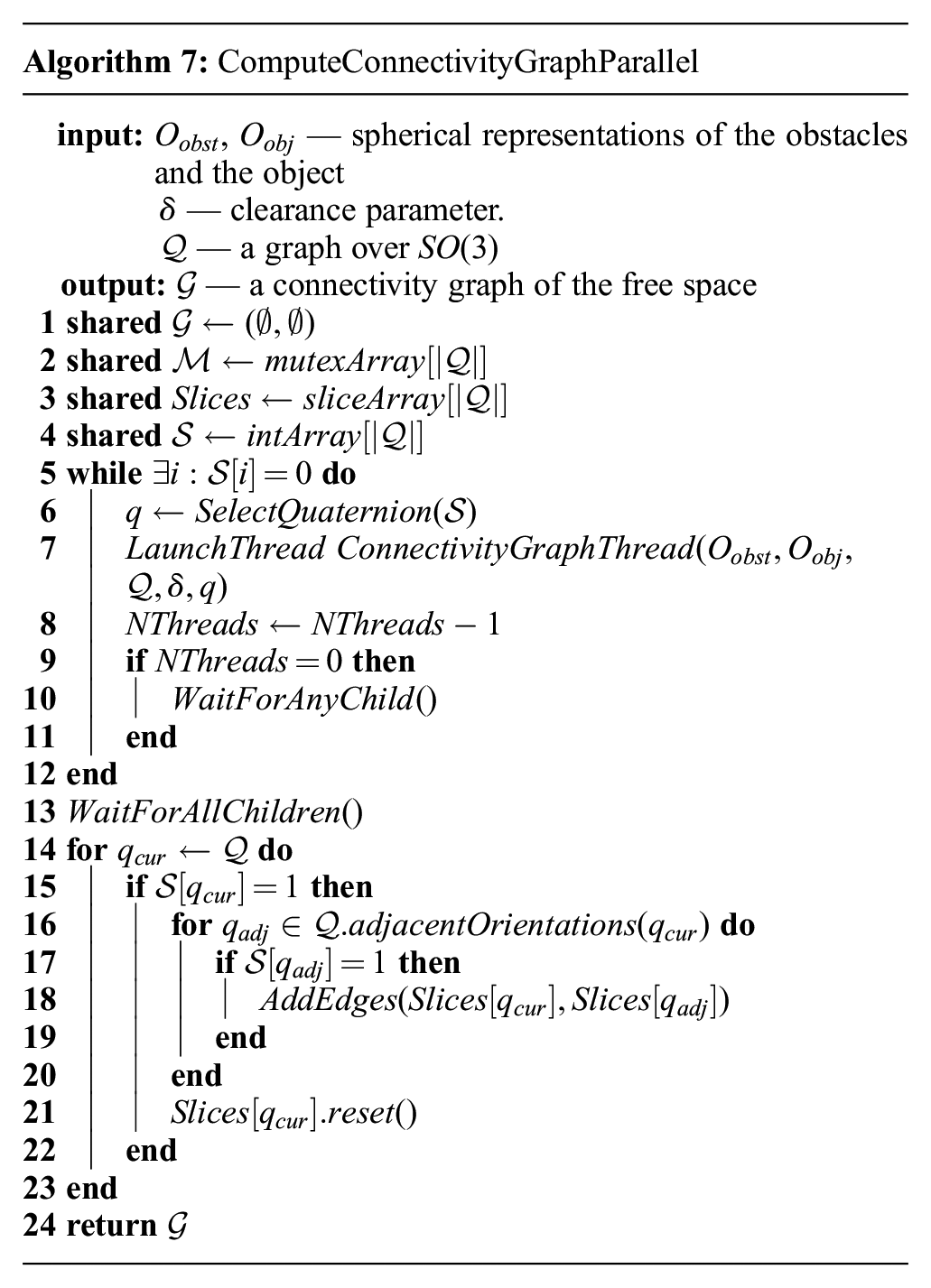
The function
8. Theoretical properties of our approach
In this section, we discuss the correctness, completeness, and computational complexity of our approach.
8.1. Correctness
First, let us show that our algorithm is correct, i.e., if there is no collision-free path between two configurations in our approximation of the free space, then these configurations are also disconnected in the actual free space.
Proof. Recall that the approximation of the free space is constructed as follows:
where
Now, recall that by definition
We now want to show that if there is no path between two vertices
Consider two adjacent slices
Let

and so
8.2.
-Completeness
Now, we show that if two configurations are not path-connected in
In proving this proposition we make used of the notion of the signed distance between two sets:
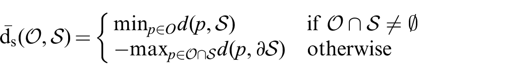
where
Proof. Recall Remark 1 that there is an edge between vertices
Recall now that we want to prove that for a pair of configurations
To see that this will result in path non-existence, we take an arbitrary

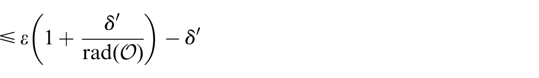
where the term
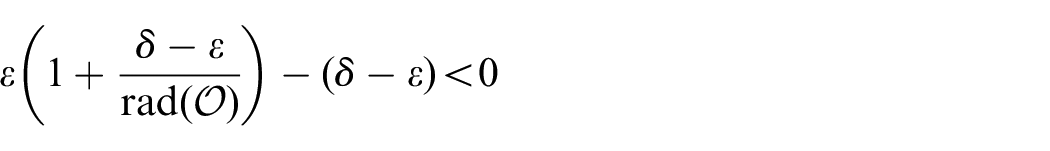
then
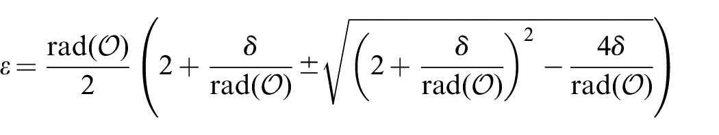
which are both positive. Finally, call the smallest of the two roots
8.3. Computational complexity
Let us now discuss the total computational complexity of the algorithm. Let
In CGAL representation, the regular triangulation contains the corresponding weighted Voronoi diagram. Note that a weighted Voronoi diagram can be constructed by other means using, for example, the algorithm from Aurenhammer and Edelsbrunner (1984). The complexity of this step is
The complexity of finding the intersections between two connected components belonging to different slices
The complexity of the final stage of the algorithm, computing connected components of the connectivity graph, is linear on the number of vertices, and can be expressed as
9. Examples and Experiments
In this section, we test our algorithm on 2D and 3D objects. In the first experiment, we investigate how the quality of the spherical approximation of the workspace affects the output of our algorithm. In the next experiment, we test our algorithm on a set of 3D objects representing different classes of geometric shapes. In our final experiment, we investigate how the performance of our parallel implementation changes with respect to different numbers of threads.
9.1. Object and obstacle approximation
A key requirement of our method is the approximation of both objects and obstacles as unions of balls. This presents a challenge, especially when dealing with 3D objects. For 2D experiments, we were able to obtain good results using a simple grid for the centers of the balls, and choosing the radius of the balls at various levels. This resulted in the approximations of the obstacle seen in Figure 6 and the results listed in Table 2, which are analyzed in the next section. Simply put, this example shows that using this approach, the smaller the radius of the balls used in the approximation the higher detail we are able to capture. However, this method can be detrimental to approximate the object, because we use an
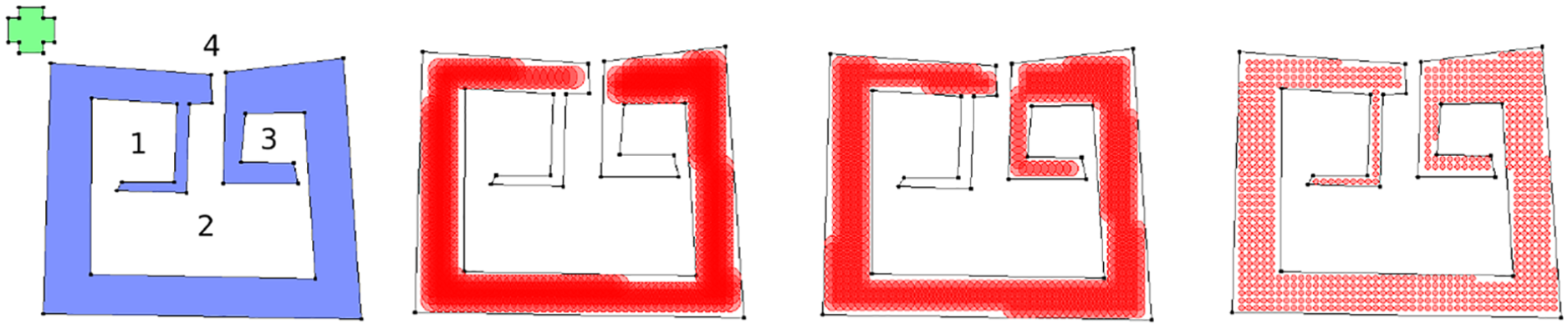
On the left we present a set of 2D obstacles in blue and an object in green. The numbers represent the connected components of the free space. In red are three approximations of the obstacles by sets of balls of radius 15, 10, and 4. Note that the smaller the radius the more features from the original configuration space are preserved. Note that the first approximation significantly simplifies the shape, and has only one narrow passage; the second approximation preserves the shape better and has two narrow passages; the third approximation preserves all the important shape features of the obstacles.
We report the number of path-connected components we found and the computation time for each case. When we were using our first approximation of the workspace, we were able to distinguish only between components 4 and 2 (see Figure 6), and therefore prove path non-existence between them. For a more accurate approximation, we were also able to detect component 3. Finally, the third approximation of the workspace allows us to prove path non-existence between every pair of the four components.
A more suitable approach to approximate the object is to compute the medial axis of the object using for example the method from Dey and Sun (2006), which is able to construct it from a pointcloud of the object. Alternatively, one can use the method from Dey and Zhao (2002), which is able to retrieve a skeleton of the object (i.e., a one-dimensional subset of the medial axis). In our experiments, we used a watertight mesh of the drill (see Figure 8) to extract its skeleton axis and obtained an approximation of the drill by sampling ball centers in the skeleton with the largest radius that did not contain any point in the mesh.
Finally, for the mug and the bugtrap (also Figure 8) we traced a slice of the object and manually fit the medial axis of the slice, which we used to create a surface of revolution where the ball centers were placed (bugtrap and body of the mug).
9.2. 2D scenario: different approximations of the workspace
In this experiment, we consider how the accuracy of a workspace spherical approximation affects the output and execution time of the algorithm, see Figure 6. This experiment was performed on a single thread of Intel Core i7 processor.
For our experiments, we generate a workspace and an object as polygons, and approximate them with unions of balls of equal radii lying strictly inside the polygons. Note that the choice of the radius is important: when it is small, we get more balls, which increases the computation time of our algorithm; on the other hand, when the radius is too large, we lose some important information about the shape of the obstacles, because narrow parts cannot be approximated by large balls, see Figure 6.
We consider a simple object whose approximation consists of five balls. We run our algorithm for all the three approximations of the workspace, and take five different values of
In our opinion, the accuracy of a workspace approximation should depend on the application scenario as well as on the amount of available computational resources.
9.3. 3D scenario: different types of 3D caging
As we have mentioned in Section 2, a number of approaches towards 3D caging is based on identifying shape features of objects and deriving sufficient caging conditions based on that. By contrast, our method is not restricted to a specific class of shapes, and the aim of this section is to consider examples of objects of different types and run our algorithm on them. The examples are depicted in Figure 7, and Table 3 reports execution times for different resolutions of the
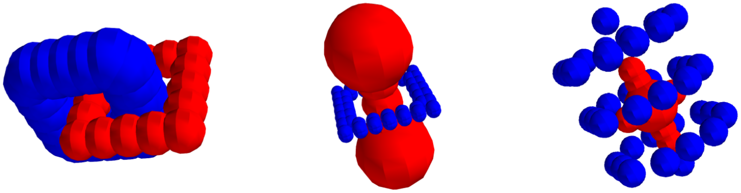
Different 3D caging scenarios. From left to right: linking-based caging (Pokorny et al., 2013; Stork et al., 2013), narrow part-based caging (Liu et al., 2018; Varava et al., 2017), surrounding-based caging.In linking-based and narrow part-based caging the obstacles form a loop (not necessarily closed) around a handle or narrow part of the object. In surrounding-based the object is surrounded by obstacles so as not to escape.
Results from running 3D experiments on the objects shown in Figure 7 using three different resolutions for the
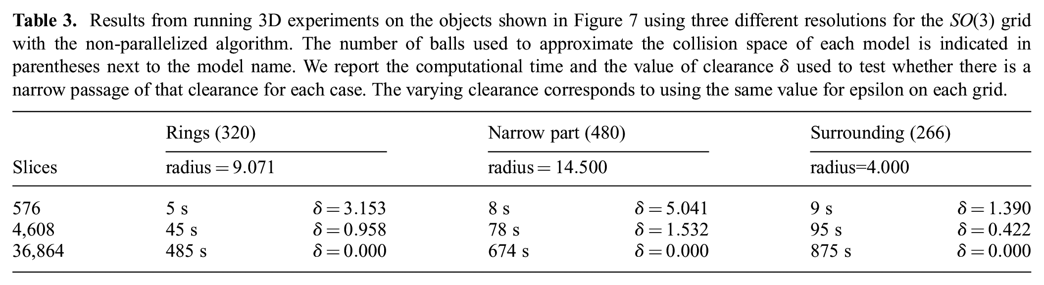
In all cases (Table 3), the object was shown to be caged when using the third grid. In the case of the narrow part example the algorithm was not able to discern a cage using the first grid. In the rings example, it was not able to find the cage with either the second or third grids.
Results that are based on low-resolution grids can in certain cases be inaccurate for two reasons. First, they have higher dispersion value, which implies that we need to use a larger value of
Another reason for inaccuracies in the low-resolution grid is the fact that the distance between neighboring orientations is so large that adjacent slices might have drastic differences in the topology of their free space. This may lead to adding edges between their connected components that would not be connected if we considered intermediate orientations as well in the case of a more fine grid.
As we see, our algorithm can be applied to different classes of shapes. It certainly cannot replace previous shape-based algorithms, as in some applications global geometric features of objects can be known a priori, in which case it might be faster and easier to make use of the available information. However, in those applications where one deals with a wide class of objects without any knowledge about shape features they might have, our algorithm provides a reasonable alternative to shape-based methods.
9.4. Parallel implementation
Our parallel implementation allows one to run experiments on more complex models of real-world objects. In this section, we consider a few objects representing different geometric features, see Figure 8. These examples are inspired by manipulation and motion planning applications. The first two models, a mug and a drill, are caged by a Schunk dexterous hand. The mug and the drill illustrate linking-based and narrow part-based caging types, respectively. The third example is a bugtrap and a small cylindrical object. The bugtrap environment is a well-known path-planning benchmark created by Parasol MP Group, CS Dept, Texas A&M University. The bugtrap does not cage the object, but contains a narrow passage. This example corresponds to the “surrounding” type of restricting the object’s mobility.
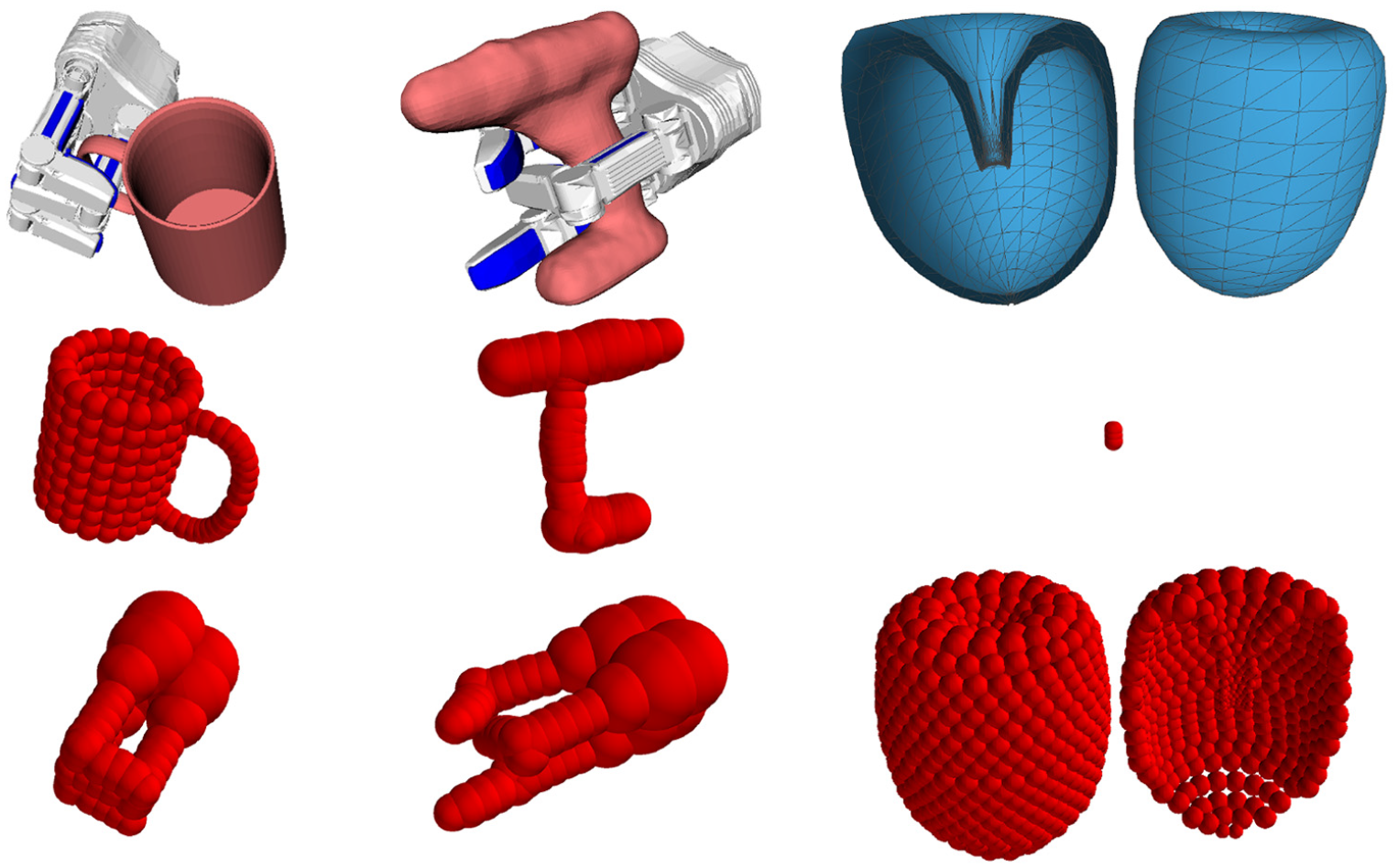
Caging real-world objects with a three-finger Schunk hand. First row, from left to right: a mug (linking-based caging), its representations as a union of balls, a drill (narrow part-based caging), a bugtrap (caging by surrounding). Second row: the respective spherical representations of the objects. Third row: a spherical representation of the Schunk hand in the caging configurations used above; an object passing through the bugtrap.
First, we observe how the performance of our algorithm changes with respect to the number of slices we consider. Table 4 reports the results. The respective objects are depicted in Figure 8. We report the computational time needed for different resolutions of the orientation grid, as well as the
Results from running 3D experiments with objects shown in Figure 8 using three different resolutions for the
Now, we analyze how the performance of the parallelized version of our algorithm changes with respect to the number of threads we use. Table 5 presents the results of this experiment. We run our algorithm using from one to eight threads on three different object models and report the respective computational time. In all examples we used 4,608 slices (second grid) and clearance
Results from running the experiments on the ring, and narrow part toy examples, as well as on the drill objects, with one to eight threads. These examples stem from using our parallel algorithm (Algorithm 7) with the objects and obstacles depicted in Figures 7 and 8, and a grid over
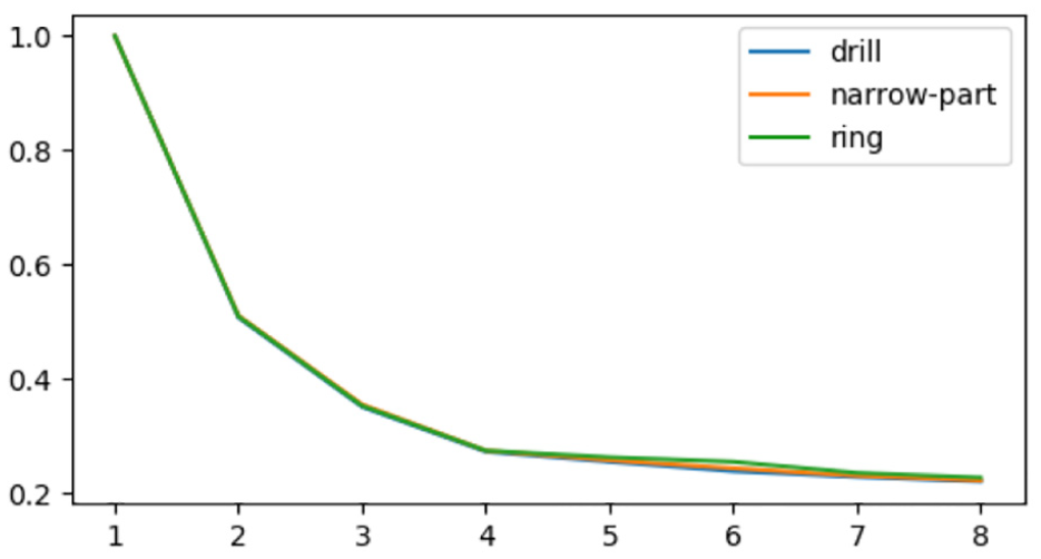
Relative timing for calculating the configuration space of objects with different numbers of threads. The vertical axis measures time in fraction of time taken by computing with a single thread. The horizontal axis indicates the number of threads. The data corresponds to that presented in Table 5.
10. Discussion and future work
In this article, we have provided a computationally feasible and provably correct algorithm for 3D and 6D configuration space approximation and used it to prove caging and path non-existence. We have analyzed the theoretical properties of the algorithm such as correctness and complexity. We have provided a parallel implementation of the algorithm, which allows us to run it on complex object models. In the future, we see several main directions of research that would build upon these results.
10.1. Molecular cages
In organic chemistry, the notion of caging was introduced independently of the concept of Mitra et al. (2013). Big molecules or their ensembles can form hollow structures with a cavity large enough to envelope a smaller molecule. Simple organic cages are relatively small in size and therefore can be used for selective encapsulation of tiny molecules based on their shape Mitra et al. (2013). In particular, this property can be used for storage and delivery of small drug molecules in living systems Rother et al. (2016). By designing the caging molecules one is able to control the formation and breakdown of a molecular cage, in such a way as to remain intact until it reaches a specific target where it will disassemble releasing the drug molecule.
An example in Figure 10 shows that, in principle, our algorithm can be applied to molecular models, assuming they can be treated as rigid bodies. In this example, we consider two molecules to see whether our algorithm can predict their ability to form a cage. Atomic coordinates and van der Waals radii were retrieved from the Cambridge Crystallographic Data Centre (CCDC) database. The depicted molecules are mesitylene (left, CCDC 907758) and CC1 (right, CCDC 707056) (Mitra et al., 2013). Our algorithm reported that this pair forms a cage, as experimentally determined in Mitra et al. (2013). In our future work, we aim to use our algorithm to test a set of potential molecular carriers and ligands to find those pairs which are likely to form cages. This prediction can later be used as a hypothesis for further laboratory experiments.
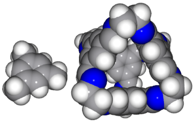
The small molecule (a guest) can be caged by the big molecule (the host).
10.2. Integration with path planners
Another possible direction of future work is integration of our approach with sampling-based path planning algorithms. Since the problems of path planning and path non-existence verification are dual to each other, we plan to design a framework where they will be addressed simultaneously: a path planner will attempt to construct a collision-free path as usual, while configuration space approximation will be constructed independently. If there is no path, our configuration space approximation can be used to rigorously demonstrate this instead of relying on heuristical stopping criteria for the planner. Furthermore, we can leverage our approximation to guide sampling, which can be particularly beneficial in the presence of narrow passages. Namely, having an approximation of the narrow regions of the free space, the planner can sample configurations from it.
10.3. Energy-bounded caging
Mahler et al. (2016, 2018) defined the concept of energy-bounded caging, when obstacles and external forces (such as gravity, or forces directly applied to the object) complement each other in restricting the object’s mobility. The authors proposed an approach towards synthesizing energy-bounded cages in two dimensions.
To directly extend their method to 3D workspaces one would need to represent the configuration space as a 6D simplicial complex, which is expensive in terms of both required memory and execution time (Mahler et al., 2016). Apart from that, the computation time in their case is dominated by sampling the collision space, and the authors suggest that in the 3D case the necessary number of samples might be even higher.
Analogously to the works by Mahler et al. (2016, 2018), we can model external forces as potential functions and assign potential values to each ball in our approximation of the free space. In each slice, we consider balls with high potential values as “forbidden” parts of the free space, and compute connected components of the rest. In the future, we plan to investigate this direction.
Footnotes
Appendix
Recall the formulation of Proposition 1.
Given two unit quaternions
Proof. For notational simplicity we divide both sides of the equation by
We proceed by reducing both sides of the equation to the same formula, starting with the left-hand side. To do this, we once again point out that we can identify quaternions with vectors in
where the last equality is due to the fact that
Furthermore, let
Substituting this into the formula, and using the Pythagorean theorem to separate the
Now we note that
Now we want to deal only with a combination of tangents, therefore we divide the term inside the square root by
Now, expanding the squares and multiplying into all the terms under the square root sign, as well as eliminating terms that cancel out, results in
By introducing an extra
Finally, recall that
Now we begin to explore the right-hand side of the equation, by noting that when
and, finally, we obtain the same formula as previously:
hence concluding the proof of Proposition 1.
Acknowledgements
The authors are grateful to D. Devaurs, L. Kavraki, and O. Kravchenko for their insights into molecular caging.
Funding
This work has been supported by the Knut and Alice Wallenberg Foundation and Swedish Research Council.