A unified framework for coordinated multi-arm motion planning

Abstract

Coordination is essential in the design of dynamic control strategies for multi-arm robotic systems. Given the complexity of the task and dexterity of the system, coordination constraints can emerge from different levels of planning and control. Primarily, one must consider task-space coordination, where the robots must coordinate with each other, with an object or with a target of interest. Coordination is also necessary in joint space, as the robots should avoid self-collisions at any time. We provide such joint-space coordination by introducing a centralized inverse kinematics (IK) solver under self-collision avoidance constraints, formulated as a quadratic program and solved in real-time. The space of free motion is modeled through a sparse non-linear kernel classification method in a data-driven learning approach. Moreover, we provide multi-arm task-space coordination for both synchronous or asynchronous behaviors. We define a synchronous behavior as that in which the robot arms must coordinate with each other and with a moving object such that they reach for it in synchrony. In contrast, an asynchronous behavior allows for each robot to perform independent point-to-point reaching motions. To transition smoothly from asynchronous to synchronous behaviors and vice versa, we introduce the notion of synchronization allocation. We show how this allocation can be controlled through an external variable, such as the location of the object to be manipulated. Both behaviors and their synchronization allocation are encoded in a single dynamical system. We validate our framework on a dual-arm robotic system and demonstrate that the robots can re-synchronize and adapt the motion of each arm while avoiding self-collision within milliseconds. The speed of control is exploited to intercept fast moving objects whose motion cannot be predicted accurately.

1. Introduction

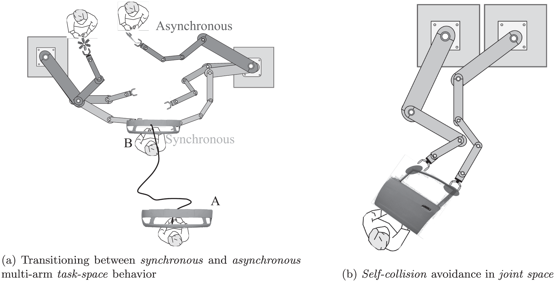
The use of multi-arm robotic systems allows for highly complex manipulation of heavy or bulky objects that would otherwise be infeasible for a single-arm robot. One can envision a plethora of applications in smart-factories or homes that would benefit from such extended workspace and capabilities. Examples include lifting, grabbing, catching, manipulating objects with multiple arms that could be either traveling on a cart or a running conveyor belt, carried by humans or even flying towards the multi-arm robot system, as depicted in Figure 1a. Moreover, a multi-arm system could provide not only synchronous behaviors, such as those mentioned above, but also asynchronous behaviors, where each robot follows its own goal-oriented task (Figure 1a). Multi-arm control strategies endowed with these capabilities can pave the way for the flexible manufacturing systems of the future.

Fig. 1.

Illustration of multi-arm task-space coordination and joint-space collision avoidance. (a) Synchronous and asynchronous task-space behaviors, where the robots coordinate with each other to simultaneously reach for a moving object or each robot has its own target and is endowed with an independent stable dynamical system to generate desired motions, respectively. (b) Self-collision avoidance (SCA) in joint space for both task-space behaviors.

The challenge is then to control these robots in a coordinated manner, in order to safely and efficiently achieve the desired manipulation task. Due to the technological difficulties that entail coordinating multiple arms with a dynamic object in a computationally efficient way, these applications have yet to be explored in the robotics community. Most effort in the field of multi-arm control has focused primarily on devising strategies for coordinated manipulation of static objects that are partially or fully grasped by the multi-arm system (Caccavale and Uchiyama, 2016). Seldom work has focused on developing coordinated strategies that a multi-arm system can use to reach and grab moving objects synchronously, while also being capable of reaching for independent targets or objects asynchronously (Vahrenkamp et al., 2012, 2010).

In this work, we draw inspiration from the field of human coordination dynamics, in order to devise safe and coordinated motions in dual/multi-arm robotic systems. Humans have a remarkable way of controlling their bi-manual movements in everyday life. They are capable of coordinating both arms and hands in synchronous and asynchronous tasks, in uni-manual and bi-manual tasks, and they transition smoothly between all of these behaviors. Interestingly, the motion of the hands, and accordingly of the arms, is generated in a smooth and efficient manner, all the while avoiding self-collisions between their limbs. Seminal works from the field of human coordination dynamics suggest that human inter-limb coordination is governed by a strongly coupled underlying non-linear dynamical system (DS) (Kelso et al., 1979; Kelso, 1984). These studies involved transitioning between in-phase and anti-phase rhythmic movements, which led to the Haken–Kelso–Bunz (HKB) model of coordination (Haken et al., 1985). Swinnen (2002) highlights strong limb-coupling in terms of the spatial constraints that govern coordination, which can be egocentric (based on mirror symmetry in muscle groups) or allocentric (following the same direction in extrinsic space). Later on, Calvin and Jirsa (2011) introduced a generalized description of such coordination dynamics, as a combination of intrinsic dynamics (coordination types) and a strong coupling between them. Showcasing that, coordination can also arise with discrete (i.e. non-rhythmic) bi-manual movements. More compelling evidence of the strong bi-manual coupling in humans can be seen when executing independent tasks. In the study of Franz et al. (1991), the subjects were asked to perform two independent discrete movements with each hand, drawing a circle and a vertical straight line, respectively. The resulting shapes were vertical ellipses, elucidating the strong ego-centric constraints in bi-manual movements.

Humans also display an underlying coordination with external agents, for example when manipulating objects. Tasks such as lifting, carrying, and reaching for large or heavy objects rely on bi-manual reaching behaviors that require not only spatial but also temporal constraints (Coats and Wann, 2012). In a bi-manual reach, each hand has to adjust to the orientation, shape, and size of the object while reaching for it. Moreover, the action of grabbing the object (i.e. closing the hands on the object) must be timed prior to rather than as a reaction to intercepting the object. Hence, bi-manual reaching requires to solve simultaneously spatial and temporal coordination constraints to move toward the object in coordination and to intercept the object (Vernon et al., 2011). Furthermore, when humans reach towards different targets, their behavior might not exhibit spatial constraints, but the temporal constraints are still enforced. They smoothly adapt their respective speed to reach the targets simultaneously. This means that there is an apparent timing synchronization even in asynchronous behaviors.

In our previous works (Salehian et al., 2016a, 2017), we offered a DS-based controller for coordinated multi-arm motion planning. The approach consists of a virtual object DS control law that generates autonomous and synchronized motions for a multi-arm robot system. We use the notion of a virtual object to both coordinate the motion of the multiple robots with each other and with a moving object, such that the robots reach the dynamic object in synchrony (Figure 1a). Such a DS emulates the strongly coupled human coordination strategies exhibited in the previously mentioned studies, providing predictable motions for humans.

In this paper, we improve upon our previous work, by tackling two main challenges that were not addressed in Salehian et al. (2016a). First, we extend the virtual object DS, such that it can generate two types of behaviors: (i) multi-arm asynchronous task-space behaviors, where each robot has its own target or desired motion (Figure 1a) and (ii) multi-arm synchronous task-space behaviors, where the robots’ task is to coordinate with each other to simultaneously reach for a moving object (Figure 1a). To provide a smooth transition between these two behaviors, we introduce the notion of synchronization allocation. Given the motion of the object and the joint workspace of the multi-arm system, each arm is being continuously allocated to a desired behavior. While being allocated to the synchronous behavior, control of the robots is taken over by the virtual object DS. While allocated to the asynchronous behavior, the robots are controlled independently, each with their own goal-directed stable DS. The proposed multi-arm DS is expressed as a linear parameter varying (LPV) system subject to stability constraints, that ensure convergence to the object or targets. Second, to ensure self-collision avoidance (SCA) at the joint-level, we propose a centralized IK solver, formulated as a constrained convex optimization problem subject to data-driven SCA constraints. These SCA constraints are introduced as linear inequality constraints in the optimization problem in the form of a continuous “SCA boundary function” and its gradient. We then propose to efficiently encode this SCA boundary function through a sparse kernel support vector machine (SVM) (Joachims and Yu, 2009), learned a priori from a simulated data set of feasible configurations of the multi-arm system. The contributions of this paper, compared with our previous work (Salehian et al., 2016a), are thus threefold.

1. Unification of synchronous and asynchronous multi-arm behaviors in a single DS.

2. A SCA IK solver formulated as a convex quadratic programming (QP) problem that can be solved in real-time.

3. A data-driven learning approach to model the SCA constraints in a computationally efficient way.

This paper is organized as follows. Section 2 highlights related work on multi-arm control and SCA strategies. In Section 3, we present the multi-arm DS, including a formalization and convergence proof of the LPV DS. Section 4 introduces a centralized inverse kinematics (IK) solver that can handle SCA constraints. In Section 5, we present the learning approach to approximate the safe manipulation regions fed to the SCA-IK solver. The proposed method is then validated with a dual-arm platform for several coordination and reaching scenarios in Section 6. Discussions and future work are presented in Section 7.

2. Related work

Coordinating multiple robotic arms for object manipulation has been studied extensively in the robotics literature, one can find comprehensive surveys on dual/multi-arm motion planning in the literature (Caccavale and Uchiyama, 2016; Smith et al., 2012; Wimböck et al., 2012; Wimböck and Ott, 2012). However, the problem of planning the reach to grasp motion for a moving object with a multi-arm robotic system, while keeping coordination constraints, is a new field of research. Only Vahrenkamp et al. (2012, 2010) tackled a similar problem, where a rapidly-exploring random tree (RRT)-based algorithm was proposed to generate collision-free motions to grasp an object at rest with a bi-manual platform. Given its search-based strategy, this approach can guarantee feasible grasps by both arms and SCA. However, due to its computational complexity and the fact that it cannot guarantee simultaneous interception of the object by all arms, it becomes inadequate when trying to reach for a moving object. Chung and Slotine (2009) proposed a contraction-based control algorithm for synchronizing multiple robotic arms with an external agent. However, the kinematic feasibility of the intercept point and the dual-behavior scenarios have not been addressed. To the best of the authors’ knowledge, there is no related work in the field of reaching for large moving objects with multi-arm systems, with the capabilities of smoothly transitioning to asynchronous behaviors, all the while avoiding for self-collision at the joint-level. Yet, for the sake of completeness, we briefly summarize works from the vast literature in multi-arm control that are relevant to each of our contributions.

2.1. De-centralized multi-arm control strategies

In de-centralized control architectures, the robots are controlled separately by their own local controllers (Liu and Arimoto, 1998). In early approaches, the coordination between a dual-arm system is achieved by categorizing them into two categories; namely a master and a slave. The motion of the master robot is assumed known whereas the slave robot must follow the master’s motion while satisfying the closed-chain geometrical constraints (Luh and Zheng, 1987). Similarly, Gams et al. (2015) proposed a control architecture to perform a task of lifting an unknown object with a dual-arm system, where the slave arm is synchronized with the master arm through a coupling guided by position and velocity feedback errors. Although computationally efficient, this strategy assumes a fixed master–slave relationship, which, when dealing with moving objects, may adversely affect performance if the arms need to switch responsibility to perform the task on-line. Bai and Wen (2010), by using a velocity feedback and force feed-forward strategy, proposed a de-centralized controller for transporting a flexible payload at a constant speed with multiple arms. In this approach master/slave roles are not assigned. However, as it assumes that each robot is a point-mass system it could not readily be applied to manipulating a moving object with unpredictable dynamics, as considered in our approach.

2.2. Centralized multi-arm control strategies

Some of the shortcomings of the de-centralized control architectures can be addressed by centralized control strategies (Aghili, 2013; Suda et al., 2003; Wang et al., 2015). These strategies consider the robots and the manipulated object as a closed kinematic chain. In this line, an impedance control architecture for dual-arm manipulation was proposed by Wimböck and Ott (2012), where the two end-effectors and a virtual frame, which is a function of the end-effectors’ poses, are coupled via spatial springs. Zhu (2005) proposed a motion synchronization controller to coordinate the end-effectors of a dual-arm system when they are rigidly or flexibly holding a massless object. In Likar et al. (2013), the motions of two robotic arms are synchronized by a velocity level motion synchronization algorithm. By concatenating the kinematic of two arms and the object, Likar et al. introduced an augmented kinematic chain. The corresponding Jacobian is calculated to control the augmented kinematic chain by solving the IK problem at the velocity level.

By exploiting advantages of centralized and de-centralized impedance control strategies, Caccavale et al. (2008) proposed a control architecture to achieve a desired impedance at both the object and the end-effector levels. Similarly, Chiacchio and Chiaverini (1998) proposed a two-level control architecture. Initially, the desired task variables are transformed into the corresponding joint-space motions by solving a centralized IK problem. Then, the desired joint motions are fed to a decentralized joint-space controller.

All previously mentioned works assume that the object is firmly attached to the robots and modeled via a virtual object frame or by closing the kinematic chain. In this work, we leverage the idea of the virtual object to address the problem of coordination. The term virtual object is mostly used in robotics literature to represent the internal forces of a grasping task (Williams and Khatib, 1993; Wimbock et al., 2008). In this paper, however, this term is used to achieve coordination at two levels. In the first level, the motion of each robot is coordinated with all robotic arms. In the second level, the resultant motion of the arms are coordinated with that of the object to satisfy the coordination constraints (i.e. for synchronous behavior).

2.3. Multi-arm SCA

Self-collision avoidance is one of the main challenges in multi-arm manipulation. It is particularly relevant in the humanoid robot community and, hence, has been studied extensively. Throughout the years, the approaches for solving collision avoidance for manipulation or locomotion in humanoids can be categorized into two types: (i) planning methods that generate feasible collision-free trajectories of known/quasi-static environments (Chrétien et al., 2016; Escande et al., 2014, 2007; Gharbi et al., 2009; Vahrenkamp et al., 2012, 2010) and (ii) reactive approaches that solve collision avoidance through the IK problem online (Fang et al., 2015; Ge and Cui, 2000; Santis et al., 2007; Sugiura et al., 2007). For a comprehensive review on collision avoidance strategies for bi-manual systems refer to Petrič et al. (2015).

The main disadvantage of planning approaches is their computational cost. Although much progress has been achieved in this regard, most planning approaches are still restricted to static scenarios. For example, in a dynamic scenario, where the robots must adapt to fast external perturbations, solving for collision avoidance must be in a matter of 1–2 ms. Typical computation times for efficient solvers in humanoid scenarios lie between $\approx 700\mathrm{ms}$ and $\approx 1\mathrm{s}$ (Kanehiro et al., 2012; Orthey and Stasse, 2013). Recently, Chrètien et al. (2016) showed that the computation time of one iteration (for their collision-avoidance humanoid trajectory solver) is 2715 ms on a single-thread CPU. They proved, however, that with the use of parallel computing, their computation time can be improved significantly, i.e. to 54 ms on a GPU. Though significant, this improvement is far from the requirements of dynamic scenarios. The sole approach that has proven to achieve dynamic adaptation at $<1$ ms is that of Murray et al. (2016), where a field programmable gate array (FPGA) robot-specific chip is designed for dynamic motion planning. Although promising, this approach is limited by the need to compute a probabilistic roadmap a priori and its dependence on a specific robot configuration.

Reactive approaches, on the other hand, are not hindered by computational inefficiency. In Santis et al. (2007) and Sugiura et al. (2007) repulsion forces were computed from colliding segments to generate SCA motions. Fang et al. (2015) proposed a hierarchical-based algorithm to find in-danger points and solve the IK problem such that the distance between these points is maximized. These approaches, although fast, suffer from the same shortcoming as generic potential-field obstacle avoidance algorithms, i.e. the stability of the generated motion is not guaranteed, as the robot might get stuck at local minima. Moreover, potential-field approaches suffer from providing no passages between closely spaced obstacles and the possibility of oscillations in the presence of obstacles (Ge and Cui, 2000).

All of the previously mentioned works, whether planning-based or reactive, have a common methodology: they rely on computing minimum distances between links/joints/segments/objects (represented as sphere/swept-spheres/polygons) to detect/avoid collisions. The use of minimum distances for collision avoidance inherently introduces non-linear and non-convex constraints to an otherwise convex optimization problem (Ratliff et al., 2015). This, in fact, is the main reason that planning algorithms rely on computationally inefficient global optimization or trajectory optimization methods and that reactive methods tend to get stuck in local minima. To this end, approaches based on signed distance fields have been successful in encoding the proximity of obstacles as continuous costs in local trajectory optimization frameworks, by either providing explicit cost gradients (Ratliff et al., 2009; Zucker et al., 2013) or through derivative-free stochastic optimization methods (Kalakrishnan et al., 2011). Such approaches, however, fail to recover when solving for optimization problems that become ill-defined due to particular shapes of obstacles or many local minima. To alleviate this, Ratliff et al. (2015) provide a general motion optimization framework that exploits the Riemannian geometry of the workspace to represent costs for obstacle avoidance, kinematic limits, etc., by warping the workspace via Riemannian metrics and their gradients. These approaches, although promising, are still limited by their computational efficiency, as they all present optimization times of $\approx 0.5\mathrm{s}$ .

In this work, we focus on solving the SCA problem efficiently, i.e. in $<2\mathrm{ms}$ . We work around the limitations of the previously mentioned approaches, by learning a continuous and continuously differentiable function $\mathrm{\Gamma }(.)$ from a data set of “collided” and “non-collided” multi-arm configurations. Here $\mathrm{\Gamma }(.)$ represents the region of feasible and infeasible robot configurations, implicitly encoding a distance in feature space, of the current robot configuration to a “collided” configuration. By formulating $\mathrm{\Gamma }(.)$ as the prediction rule of a kernel SVM (Scholkopf and Smola, 2001) we can compute a continuous $\nabla \mathrm{\Gamma }(.)$ on-line. We hence propose a centralized IK solver as a convex QP optimization problem subject to linear inequality constraints imposed by $\mathrm{\Gamma }(.)$ and $\nabla \mathrm{\Gamma }(.)$ , avoiding (i) the computation of $\min (\parallel .{\parallel }_2)$ pair-wise distances between joints/links/segments and (ii) the need for trajectory optimization. Through the use of a sparse SVM approximation (Joachims and Yu, 2009) we learn an efficient representation of $\mathrm{\Gamma }(.)$ that enables us to solve the QP optimization problem in less than 2 ms, implemented on a single-threaded CPU.

3. Coordinated multi-arm motion planning

In order to achieve the envisioned scenario, i.e. smoothly transition between asynchronous and synchronous behaviors depending on the object’s motion, two main challenges should be addressed:

1. prediction of the object’s trajectory and computation of its feasible intercept points;

2. planning stable multi-arm motions towards their corresponding object intercept points (when allocated to synchronous behavior) or individual targets (when allocated to asynchronous behavior).

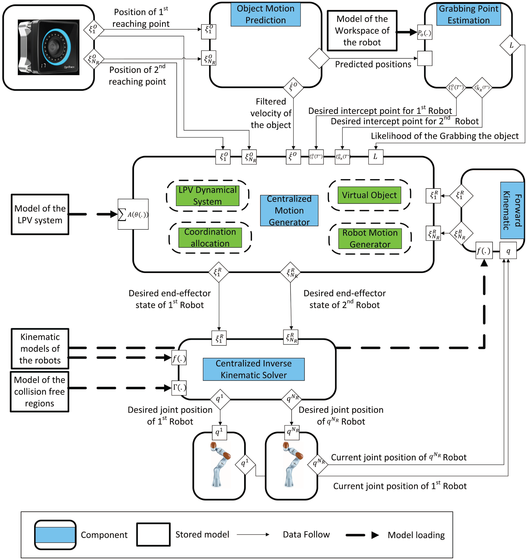
The proposed solutions to these challenges are described in Sections 3.1 and 3.2, respectively. Once the multiple end-effector motions are generated, these are mapped to desired joint-space configurations by a centralized IK solver that uses a learned model of collision-free regions and the robots’ kinematic constraints, as described in Sections 4 and 5. For simplicity and practicality, we summarize the most relevant notations used throughout the paper in Table 1 and illustrate them in Figure 2. The control flow of the entire framework is illustrated in Figure 3.

Table 1.

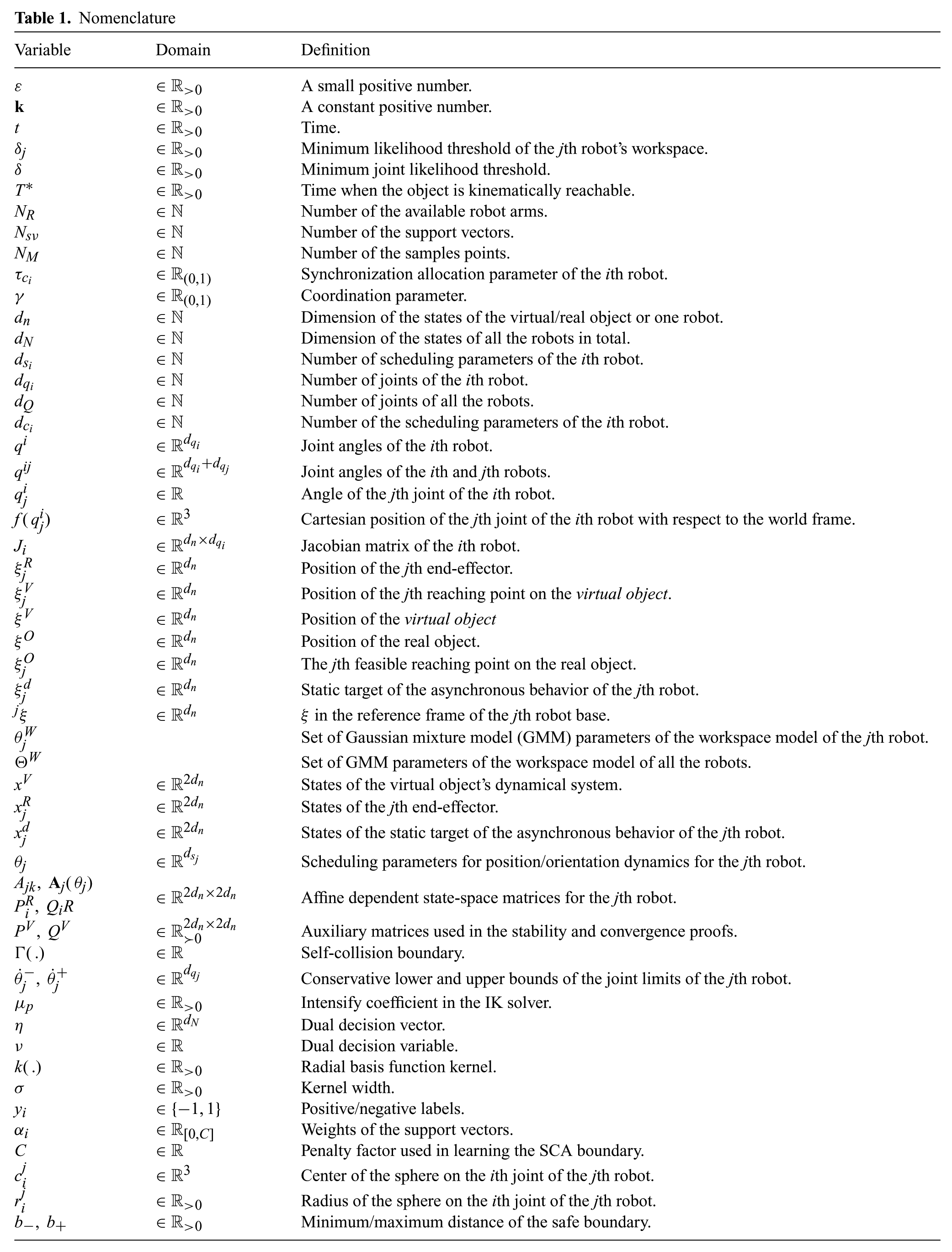
Nomenclature

Variable	Domain	Definition
$\epsilon$	$\in {\mathrm{ℝ}}_{>0}$	A small positive number.
$k$	$\in {\mathrm{ℝ}}_{>0}$	A constant positive number.
$t$	$\in {\mathrm{ℝ}}_{>0}$	Time.
${\delta }_j$	$\in {\mathrm{ℝ}}_{>0}$	Minimum likelihood threshold of the $j$ th robot’s workspace.
$\delta$	$\in {\mathrm{ℝ}}_{>0}$	Minimum joint likelihood threshold.
$T^{*}$	$\in {\mathrm{ℝ}}_{>0}$	Time when the object is kinematically reachable.
$N_R$	$\in \mathrm{\mathbb{N}}$	Number of the available robot arms.
$N_{s\nu }$	$\in \mathrm{\mathbb{N}}$	Number of the support vectors.
$N_M$	$\in \mathrm{\mathbb{N}}$	Number of the samples points.
${\tau }_{c_i}$	$\in {\mathrm{ℝ}}_{(0,1)}$	Synchronization allocation parameter of the $i$ th robot.
$\gamma$	$\in {\mathrm{ℝ}}_{(0,1)}$	Coordination parameter.
$d_n$	$\in \mathrm{\mathbb{N}}$	Dimension of the states of the virtual/real object or one robot.
$d_N$	$\in \mathrm{\mathbb{N}}$	Dimension of the states of all the robots in total.
$d_{s_i}$	$\in \mathrm{\mathbb{N}}$	Number of scheduling parameters of the $i$ th robot.
$d_{q_i}$	$\in \mathrm{\mathbb{N}}$	Number of joints of the $i$ th robot.
$d_Q$	$\in \mathrm{\mathbb{N}}$	Number of joints of all the robots.
$d_{c_i}$	$\in \mathrm{\mathbb{N}}$	Number of the scheduling parameters of the $i$ th robot.
$q^i$	$\in {\mathrm{ℝ}}^{d_{q_i}}$	Joint angles of the $i$ th robot.
$q^{ij}$	$\in {\mathrm{ℝ}}^{d_{q_i}+d_{q_j}}$	Joint angles of the $i$ th and $j$ th robots.
$q_j^i$	$\in \mathrm{ℝ}$	Angle of the $j$ th joint of the $i$ th robot.
$f(q_j^i)$	$\in {\mathrm{ℝ}}^3$	Cartesian position of the $j$ th joint of the $i$ th robot with respect to the world frame.
$J_i$	$\in {\mathrm{ℝ}}^{d_n\times d_{q_i}}$	Jacobian matrix of the $i$ th robot.
${\xi }_j^R$	$\in {\mathrm{ℝ}}^{d_n}$	Position of the $j$ th end-effector.
${\xi }_j^V$	$\in {\mathrm{ℝ}}^{d_n}$	Position of the $j$ th reaching point on the virtual object.
${\xi }^V$	$\in {\mathrm{ℝ}}^{d_n}$	Position of the virtual object
${\xi }^O$	$\in {\mathrm{ℝ}}^{d_n}$	Position of the real object.
${\xi }_j^O$	$\in {\mathrm{ℝ}}^{d_n}$	The $j$ th feasible reaching point on the real object.
${\xi }_j^d$	$\in {\mathrm{ℝ}}^{d_n}$	Static target of the asynchronous behavior of the $j$ th robot.
${}^j\xi$	$\in {\mathrm{ℝ}}^{d_n}$	$\xi$ in the reference frame of the $j$ th robot base.
${\theta }_j^W$		Set of Gaussian mixture model (GMM) parameters of the workspace model of the $j$ th robot.
${\mathrm{\Theta }}^W$		Set of GMM parameters of the workspace model of all the robots.
$x^V$	$\in {\mathrm{ℝ}}^{2d_n}$	States of the virtual object’s dynamical system.
$x_j^R$	$\in {\mathrm{ℝ}}^{2d_n}$	States of the $j$ th end-effector.
$x_j^d$	$\in {\mathrm{ℝ}}^{2d_n}$	States of the static target of the asynchronous behavior of the $j$ th robot.
${\theta }_j$	$\in {\mathrm{ℝ}}^{d_{s_j}}$	Scheduling parameters for position/orientation dynamics for the $j$ th robot.
$A_{jk},A_j({\theta }_j)$
	$\in {\mathrm{ℝ}}^{2d_n\times 2d_n}$	Affine dependent state-space matrices for the $j$ th robot.
$P_i^R,Q_{i}R$
$P^V,Q^V$	$\in {\mathrm{ℝ}}_{\succ 0}^{2d_n\times 2d_n}$	Auxiliary matrices used in the stability and convergence proofs.
$\mathrm{\Gamma }(.)$	$\in \mathrm{ℝ}$	Self-collision boundary.
${\stackrel{.}{\theta }}_j^{-},{\stackrel{.}{\theta }}_j^{+}$	$\in {\mathrm{ℝ}}^{d_{q_j}}$	Conservative lower and upper bounds of the joint limits of the $j$ th robot.
${\mu }_p$	$\in {\mathrm{ℝ}}_{>0}$	Intensify coefficient in the IK solver.
$\eta$	$\in {\mathrm{ℝ}}^{d_N}$	Dual decision vector.
$\nu$	$\in \mathrm{ℝ}$	Dual decision variable.
$k(.)$	$\in {\mathrm{ℝ}}_{>0}$	Radial basis function kernel.
$\sigma$	$\in {\mathrm{ℝ}}_{>0}$	Kernel width.
$y_i$	$\in \{-1,1\}$	Positive/negative labels.
${\alpha }_i$	$\in {\mathrm{ℝ}}_{[0,C]}$	Weights of the support vectors.
$C$	$\in \mathrm{ℝ}$	Penalty factor used in learning the SCA boundary.
$c_i^j$	$\in {\mathrm{ℝ}}^3$	Center of the sphere on the $i$ th joint of the $j$ th robot.
$r_i^j$	$\in {\mathrm{ℝ}}_{>0}$	Radius of the sphere on the $i$ th joint of the $j$ th robot.
$b_{-},b_{+}$	$\in {\mathrm{ℝ}}_{>0}$	Minimum/maximum distance of the safe boundary.

Fig. 2.

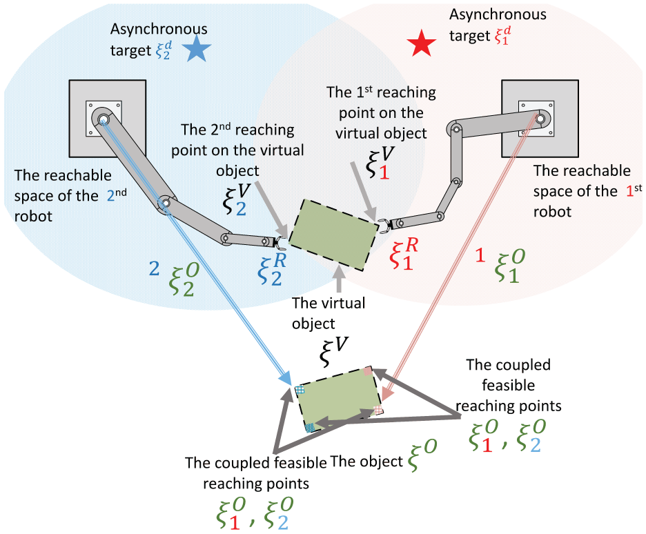
An illustration of the variables for $N_R=2$ . The reachable areas are feasible areas for grasping the object. Except for ${{}^2\xi }_2^O$ and ${{}^1\xi }_1^O$ , the variables are expressed in the reference frame located on the desired intercept point, i.e. ${\xi }^O(T^{*})=[0\dots {0]}^{\mathrm{T}}$ .

Fig. 3.

Block diagram for coordinated multi-arm motion planning for reaching a large moving object. Here $N_R$ represents the total number of robot arms and $T$ represents the motion prediction duration. In this paper, we assume that the low-level controller of the robot is a perfect tracking controller.

3.1. Object trajectory and intercept-point prediction

Once the main object starts moving towards the robots, a linear model predicts its progress ahead of time and determines a point along its trajectory where the object will become reachable by all robotic arms. We do not assume a known model of the dynamics of the object. The sole knowledge about the object is the location of its reaching points. These correspond to the user-defined position and orientation of the arms at the reaching point (see Figure 2).

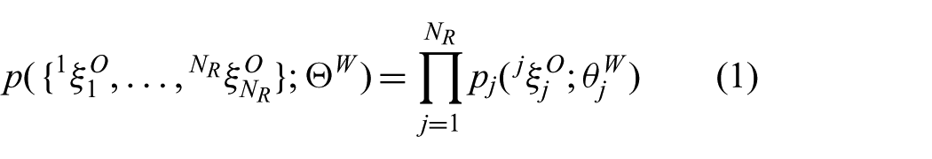
To find the feasible intercept point, which is the point where the object can be reached by all robots, at its pre-defined reaching points, we model the workspace of each robot via a probabilistic classification scheme. The reachable workspace of each robot, $p_j(\xi ;{\theta }_j^W)\forall j\in \{1,\dots ,N_R\}$ for $N_R$ robots, is modeled through a Gaussian mixture model (Bishop, 2007). If $p_j{(}^j{\xi }_i^O)>{\delta }_j$ , where ${\delta }_j$ is a minimum likelihood threshold, then ${{}^j\xi }_i^O$ , i.e. the $i$ th reaching position on the object (sub-script) in the $j$ th robot’s reference frame (left super-script), is classified as a feasible position for the $j$ th robot to reach. As the reachable workspaces of each robot are statistically independent of each other, we can calculate the joint distribution of all workspaces by computing the product of distributions, as follows:

$$p(\{{{}^1\xi }_1^O,\dots ,{{}^{N_R}\xi }_{N_R}^O\};{\mathrm{\Theta }}^W)={\displaystyle \prod _{j=1}^{N_R}}{p}_j({{}^j\xi }_j^O;{\theta }_j^W)$$

(1)

where ${\mathrm{\Theta }}^W=\{{\theta }_1^W,\dots ,{\theta }_{N_R}^W\}$ is the set of parameters for all robot workspaces and $\{{{}^1\xi }_1^O,\dots ,{{}^{N_R}\xi }_{N_R}^O\}$ are the reaching positions in each robot’s reference frame. The minimum joint likelihood threshold is $\delta ={\displaystyle {\prod }_{j=1}^{N_R}}{\delta }_j$ . if $\exists T^{*}:\delta <p({{}^1\xi }_1^O(T^{*}),\dots ,{{}^{N_R}\xi }_{N_R}^O(T^{*});\mathrm{\Theta })$ , the object at $T^{*}$ $({\xi }^O(T^{*})=\frac{1}{N_R}{\displaystyle \sum _{j=1}^{N_R}}{\xi }_j^O(T^{*}))$ is classified as the feasible intercept point. If more than one point on the predicted trajectory is classified as the feasible intercept point, we select the closest one, in Euclidean space position, to the robot end-effectors. Refer to Salehian et al. (2016a) for details of this procedure.

3.2. DS-based control of multi-arm systems

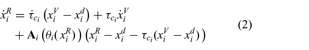
Once the feasible intercept point is found, the motion of the $i$ th robot’s end-effector $\forall i\in \{1,\dots ,N_R\}$ , is generated by following a LPV DS, composed of both synchronous and asynchronous behaviors, and coupled to the motion of the object ( ${\xi }^O$ ) through a virtual object $\left({\xi }^V\right)$ (see Figure 4) as follows:

$$\begin{array}{c}{\stackrel{.}{x}}_i^R={\stackrel{.}{\tau }}_{c_i}\left(x_i^V-x_i^d\right)+{\tau }_{c_i}{\stackrel{.}{x}}_i^V\hfill \\ +A_i\left({\theta }_i(x_i^R)\right)\left(x_i^R-x_i^d-{\tau }_{c_i}(x_i^V-x_i^d)\right)\hfill \end{array}$$

(2)

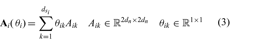
where $x_i^R(t)={\left[\begin{array}{cc}{\xi }_i^R\hfill & {\stackrel{.}{\xi }}_i^R\hfill \end{array}\right]}^{\mathrm{T}}\in {\mathrm{ℝ}}^{2d_n}$ and $x_i^V(t)={\left[\begin{array}{cc}{\xi }_i^V\hfill & {\stackrel{.}{\xi }}_i^V\hfill \end{array}\right]}^{\mathrm{T}}\in {\mathrm{ℝ}}^{2d_n}$ are the state of the $i$ th end-effector and virtual object, respectively. ¹ The state of the virtual object is used to guide the robots for synchronous behaviors. In the case of asynchronous behaviors, each $i$ th robot has its own static target, denoted as $x_i^d=\left[\begin{array}{cc}{\xi }_i^d\hfill & 0\hfill \end{array}\right]\in {\mathrm{ℝ}}^{2d_n}$ . Here $0\le {\tau }_{c_i}\le 1$ is the synchronization allocation parameter and is of class ${\mathcal{C}}^1$ and ${\theta }_i(x_i^R)\in {\mathrm{ℝ}}^{d_{s_i}\times 1}\forall i\in \{1,\dots N_R\}$ is a vector of scheduling parameters, ${\theta }_i(x_i^R)={\left[\begin{array}{ccc}{\theta }_{i1}(x_i^R)\hfill & \dots \hfill & {\theta }_{i{d}_{s_i}}(x_i^R)\hfill \end{array}\right]}^{\mathrm{T}}$ and for simplicity of notation, its argument is dropped in the rest of the paper. We use $A_i(.):{\mathrm{ℝ}}^{d_{s_i}\times 1}\to {\mathrm{ℝ}}^{2d_n\times 2d_n}$ to denote the affine dependence of state-space matrices on the scheduling parameter and the state vectors:

$$\begin{array}{lll}{A}_i({\theta }_i)={\displaystyle \sum _{k=1}^{d_{s_i}}}{\theta }_{ik}{A}_{ik}\hfill & A_{ik}\in {\mathrm{ℝ}}^{2d_n\times 2d_n}\hfill & {\theta }_{ik}\in {\mathrm{ℝ}}^{1\times 1}\hfill \end{array}$$

(3)

Fig. 4.

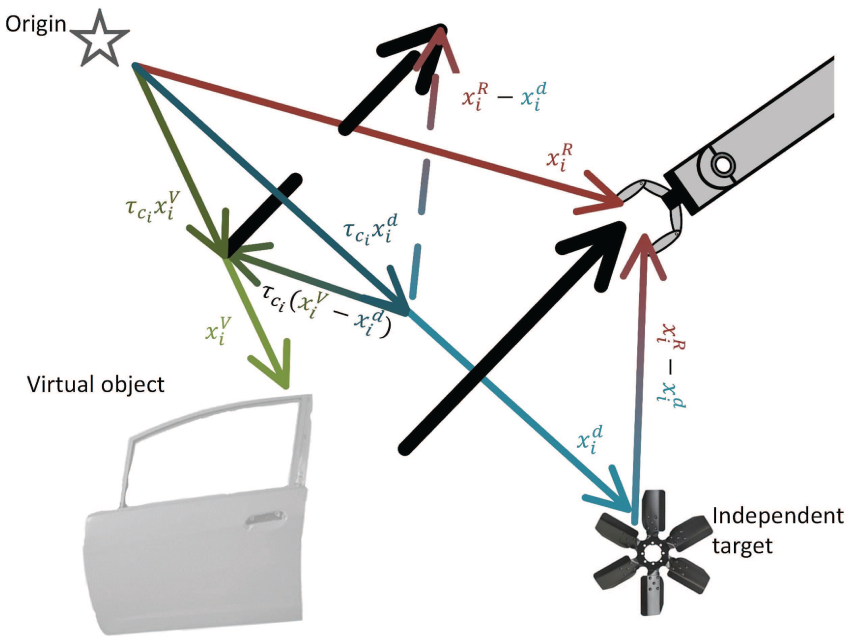
An illustration of the variables in (2). The colors of the variables and the arrows are corresponding, i.e. red represents the arm, green represents the virtual object, and blue represents the independent target. The black arrows illustrates $(x_i^R-x_i^d-{\tau }_{c_i}(x_i^V-x_i^d))$ . The dashed lines are used to show how the resultant vector is calculated.

The parameters of LPV systems can be approximated with regression models, i.e. polynomial, periodic functions, or Gaussian mixture regression (GMR). In this paper, the latter approach is used to approximate the scheduling parameters from kinematically feasible demonstrations. The advantage of this technique is that it inherently results in normalized scheduling parameters, i.e. $0<{\theta }_{ik}\le 1,$ ${\displaystyle {\sum }_{k=1}^{d_{s_i}}}{\theta }_{ik}=1$ , $\forall i\in \{1,\dots ,N_R\}$ , refer to Salehian et al. (2016b) for further details on this approximation approach.

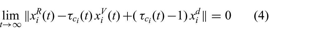
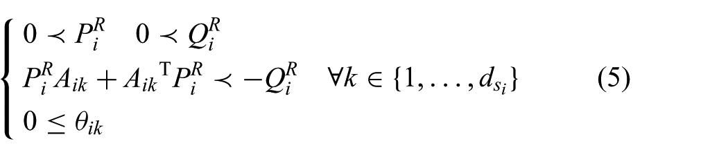
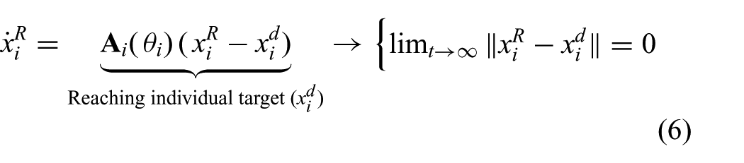
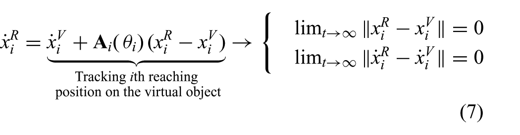
Theorem 1. The DSs given by (2) asymptotically converge to ${\tau }_{c_i}{x}_i^V+(1-{\tau }_{c_i})x_i^d$ , i.e.

$$\underset{t\to \infty }{{\displaystyle \lim }}\parallel x_i^R(t)-{\tau }_{c_i}(t)x_i^V(t)+({\tau }_{c_i}(t)-1)x_i^d\parallel =0$$

(4)

if there exist $P_i^R,Q_i^R$ such that

$$(\begin{array}{c}\begin{array}{l}0\prec P_i^{R}0\prec Q_i^R\hfill \\ P_i^R{A}_{ik}+{A_{ik}}^{\mathrm{T}}{P}_i^R\prec -Q_i^R\hfill \\ 0\le {\theta }_{ik}\hfill \end{array}\forall k\in \{1,\dots ,d_{s_i}\}\hfill \end{array}$$

(5)

Moreover, by taking ${\stackrel{.}{\tau }}_{c_i}(x_i^V-x_i^d)+{\tau }_{c_i}{\stackrel{.}{x}}_i^V-A_i({\theta }_i(x_i^R))(x_i^d+{\tau }_{c_i}(x_i^V-x_i^d))$ as the input and $x_i^R(t)$ as the output of the DS (2), Equation (2) is passive if (5) is satisfied.

Proof: See Appendices B and C.

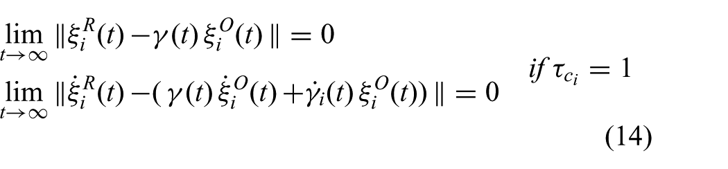
In (5), $P_i^R$ and $Q_i^R$ are auxiliary matrices that are used in a Lyapunov stability and convergence proof provided in Appendix B. It is important to remark that the Lyapunov function used in these stability proofs and, hence, the matrices $P_i^R$ and $Q_i^R$ , are never evaluated, since it is merely their existence that is required. In (2), ${\tau }_{c_i}$ determines the level of synchronization between the $i$ th robot and the virtual object, see Figure 4. Assuming that ${\tau }_{c_i}$ is constant and (5) is satisfied, when ${\tau }_{c_i}=0$ , Equation (2) yields an asynchronous DS for reaching towards individual targets:

$$\begin{array}{l}{\stackrel{.}{x}}_i^R=\underset{\mathrm{Reaching\; individual\; target}(x_i^d)}{\underbrace{A_i({\theta }_i)(x_i^R-x_i^d)}}\to (\begin{array}{c}{\lim }_{t\to \infty }\parallel x_i^R-x_i^d\parallel =0\hfill \end{array}\hfill \end{array}$$

(6)

Similarly, when ${\tau }_{c_i}=1$ , Equation (2) results in a perfect tracking DS of the $i$ th reaching point on the virtual object:

$$\begin{array}{l}{\stackrel{.}{x}}_i^R=\underset{\begin{array}{c}\mathrm{Tracking}i\mathrm{th\; reaching}\hfill \\ \mathrm{position\; on\; the\; virtual\; object}\hfill \end{array}}{\underbrace{{\stackrel{.}{x}}_i^V+A_i({\theta }_i)(x_i^R-x_i^V)}}\to (\begin{array}{c}{\lim }_{t\to \infty }\parallel x_i^R-x_i^V\parallel =0\hfill \\ {\lim }_{t\to \infty }\parallel {\stackrel{.}{x}}_i^R-{\stackrel{.}{x}}_i^V\parallel =0\hfill \end{array}\hfill \end{array}$$

(7)

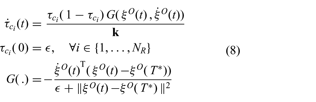
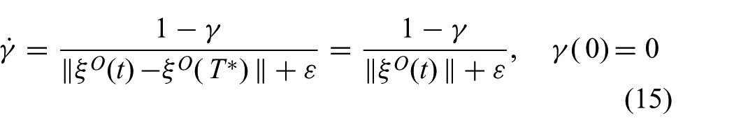
To smoothly transition between these behaviors, one could calculate ${\tau }_{c_i}\forall i\in \{1,\dots ,N_R\}$ with a continuous logistic function. In this paper, however, we propose the following DS that varies ${\tau }_{c_i}\forall i\in \{1,\dots ,N_R\}$ such that ${\tau }_{c_i}\to 1$ when the object moves towards the robots and ${\tau }_{c_i}\to 0$ when it moves away:

$$\begin{array}{c}{\stackrel{.}{\tau }}_{c_i}(t)=\frac{{\tau }_{c_i}(1-{\tau }_{c_i})G({\xi }^O(t),{\stackrel{.}{\xi }}^O(t))}{k}\hfill \\ {\tau }_{c_i}(0)=ϵ,\forall i\in \{1,\dots ,N_R\}\hfill \\ G(.)=-\frac{{\stackrel{.}{\xi }}^O{(t)}^{\mathrm{T}}({\xi }^O(t)-{\xi }^O(T^{*}))}{ϵ+\parallel {\xi }^O(t)-{\xi }^O(T^{*}){\parallel }^2}\hfill \end{array}$$

(8)

where $0<ϵ\ll 1$ is a small positive value, $k\in {\mathrm{ℝ}}_{>0}$ is a positive constant that controls for the steepness of the increase or decrease of the parameter. ² As the initial value of ${\tau }_{c_i}$ is positive $<1$ , Equation (8) is a bounded DS between $[0,1]$ . Here $G(.)$ is a function that coordinates the robots with the virtual object, such that if the real object moves toward the workspaces, the robots perform the synchronous behavior, otherwise they fall back to the asynchronous behavior. The main advantage of the proposed criterion is its adaptability. Here $\mathrm{sgn}({\tau }_{c_i})$ changes with respect to the direction of the object’s motion: when the object approaches the robots, $\mathrm{sgn}({\tau }_{c_i})\to (+)$ ; otherwise, $\mathrm{sgn}({\tau }_{c_i})\to (-)$ . Consequently, if the object is moving towards the robots, they are synchronized with the virtual object. Otherwise, they perform the asynchronous behavior.

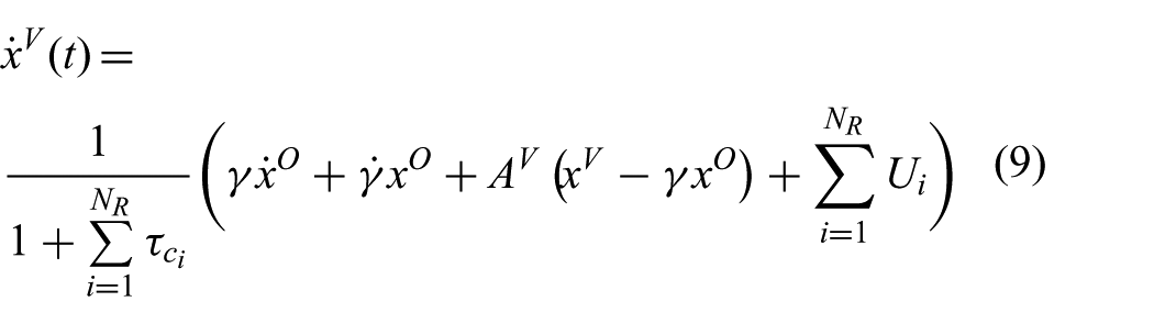
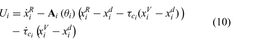
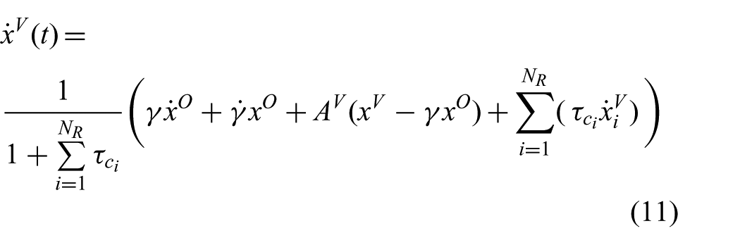
As the synchronization allocation parameters vary over time, the virtual object DS proposed in Salehian et al. (2016a), which generates the motion of the virtual object, is no longer applicable. To appropriately consider the effects of the synchronization parameters on the motion of the virtual object, and consequently of the robots, the following DS is proposed to generate the motion of the virtual object:

$$\begin{array}{l}{\stackrel{.}{x}}^V(t)=\hfill \\ \frac{1}{1+{\displaystyle \sum _{i=1}^{N_R}}{\tau }_{c_i}}(\gamma {\stackrel{.}{x}}^O+\stackrel{.}{\gamma }{x}^O+A^V\left(x^V-\gamma x^O\right)+{\displaystyle \sum _{i=1}^{N_R}}{U}_i)\hfill \end{array}$$

(9)

where $x^V(t)=\left[\begin{array}{cc}{\xi }^V(t)\hfill & {\stackrel{.}{\xi }}^V(t)\hfill \end{array}\right]$ is the state of the virtual object, $0<\gamma <1$ is the coordination parameter and is of class ${\mathcal{C}}^1$ , and $U_i$ is the interaction effect of the motion of the $i$ th end-effector on the virtual object, based on (2) and (9):

$$\begin{array}{c}{U}_i={\stackrel{.}{x}}_i^R-A_i\left({\theta }_i\right)\left(x_i^R-x_i^d-{\tau }_{c_i}(x_i^V-x_i^d)\right)\hfill \\ -{\stackrel{.}{\tau }}_{c_i}\left(x_i^V-x_i^d\right)\hfill \end{array}$$

(10)

By substituting (2) and (10) into (9), we have

$$\begin{array}{l}{\stackrel{.}{x}}^V(t)=\hfill \\ \frac{1}{1+{\displaystyle \sum _{i=1}^{N_R}}{\tau }_{c_i}}(\gamma {\stackrel{.}{x}}^O+\stackrel{.}{\gamma }{x}^O+A^V(x^V-\gamma x^O)+{\displaystyle \sum _{i=1}^{N_R}}({\tau }_{c_i}{\stackrel{.}{x}}_i^V))\hfill \end{array}$$

(11)

Theorem 2. The DS given by (11) asymptotically converges to ${\left[\begin{array}{cc}\gamma (t){\xi }^O(t)\hfill & \gamma (t){\stackrel{.}{\xi }}^O(t)+\stackrel{.}{\gamma }(t){\xi }^O(t)\hfill \end{array}\right]}^{\mathrm{T}}$ , i.e.

$$\begin{array}{l}\underset{t\to \infty }{{\displaystyle \lim }}\parallel {\xi }^V(t)-\gamma (t){\xi }^O(t)\parallel =0\hfill \\ \underset{t\to \infty }{{\displaystyle \lim }}\parallel {\stackrel{.}{\xi }}^V(t)-(\gamma (t){\stackrel{.}{\xi }}^O(t)+\stackrel{.}{\gamma }(t){\xi }^O(t))\parallel =0\hfill \end{array}$$

(12)

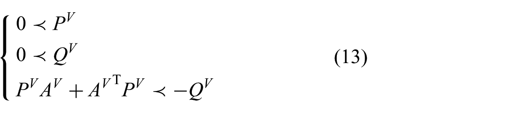
if there exist $P_i^V,Q_i^V$ such that

$$\{\begin{array}{c}\begin{array}{l}0\prec P^V\hfill \\ 0\prec Q^V\hfill \\ P^V{A}^V+{A^V}^{\mathrm{T}}{P}^V\prec -Q^V\hfill \end{array}\hfill \end{array}$$

(13)

Moreover, by taking $\gamma {\stackrel{.}{x}}^O+\stackrel{.}{\gamma }{x}^O-A^V(\gamma x^O)$ as the input and $x^V$ as the output of the DS (11), Equation (11) is passive if (13) is satisfied.

Proof: See Appendices D and E.

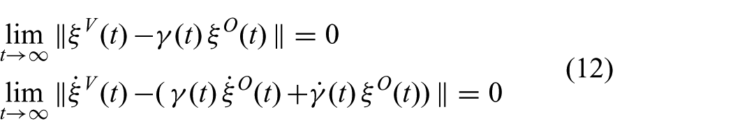
Remark 1. If ${\tau }_{c_i}=1$ , based on (7) and (12), the robots asymptotically converge to the reaching points on the object, i.e.

$$\begin{array}{l}\underset{t\to \infty }{{\displaystyle \lim }}\parallel {\xi }_i^R(t)-\gamma (t){\xi }_i^O(t)\parallel =0\hfill \\ \underset{t\to \infty }{{\displaystyle \lim }}\parallel {\stackrel{.}{\xi }}_i^R(t)-(\gamma (t){\stackrel{.}{\xi }}_i^O(t)+{\stackrel{.}{\gamma }}_i(t){\xi }_i^O(t))\parallel =0\hfill \end{array}if{\tau }_{c_i}=1$$

(14)

In (13), $P_i^V$ and $Q_i^V$ are auxiliary matrices that are used in the stability and convergence proof; see Appendix D. If ${\tau }_{c_i}=1$ and $\left(\gamma (t)=\stackrel{.}{\gamma }(t)=0\right)$ , Equation (11) generates asymptotically stable motions towards the predicted intercept point, i.e. coordination between the robots is preserved, but the coordination between the robots and the object is lost. If ${\tau }_{c_i}=1$ and $\left(\gamma (t)=1,\stackrel{.}{\gamma }(t)=0\right)$ , Equation (11) generates asymptotically stable motions towards the real object, even though its motion is not accurately predicted, i.e. perfect coordination with the object. ³ However, in this case, there is no guarantee that the virtual object intercepts the real object inside the workspace of the robots, i.e. because of the robots’ kinematic constraints, the coordination between them is lost. Thus, one can vary the values of the coordination parameters between $[0,1]$ , such that $\gamma =1$ at the vicinity of the desired intercept time as proposed in Salehian et al. (2016a):

$$\stackrel{.}{\gamma }=\frac{1-\gamma }{\parallel {\xi }^O(t)-{\xi }^O(T^{*})\parallel +\epsilon }=\frac{1-\gamma }{\parallel {\xi }^O(t)\parallel +\epsilon },\gamma (0)=0$$

(15)

Equation (15) improves the robustness of the multi-arm reaching motion in the face of inaccuracies in the object’s motion prediction, as it ensures that when the object is close enough to the feasible reaching positions, the virtual object converges to the real object and perfectly tracks it, i.e. $\gamma (T^{*})=1$ . Hence, the robots can simultaneously track the desired reaching points on the object in coordination. The C++ implementation of this approach is provided in Multiarm_ds (Table 2). The proposed algorithm can only guarantee collision-avoidance between end-effectors, via the virtual object, for synchronous behaviors. In the following section we present a centralized IK solver, that addresses SCA at all times.

Table 2.

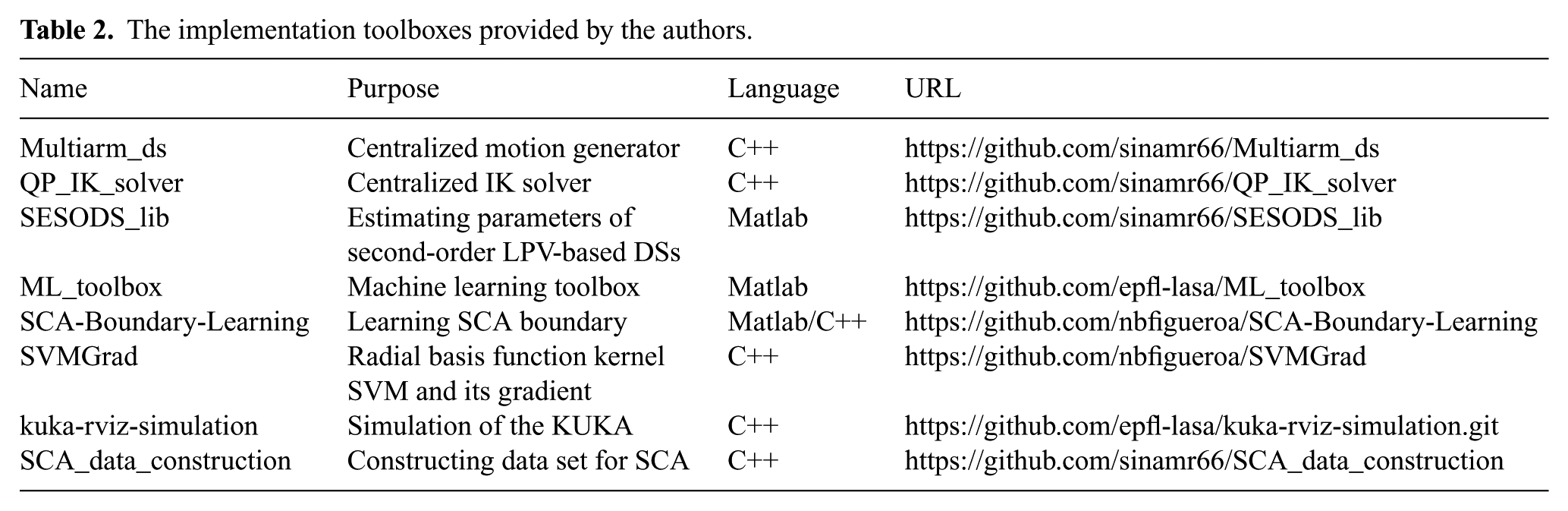
The implementation toolboxes provided by the authors.

Name	Purpose	Language	URL
Multiarm_ds	Centralized motion generator	C++	https://github.com/sinamr66/Multiarm_ds
QP_IK_solver	Centralized IK solver	C++	https://github.com/sinamr66/QP_IK_solver
SESODS_lib	Estimating parameters of	Matlab	https://github.com/sinamr66/SESODS_lib
	second-order LPV-based DSs
ML_toolbox	Machine learning toolbox	Matlab	https://github.com/epfl-lasa/ML_toolbox
SCA-Boundary-Learning	Learning SCA boundary	Matlab/C++	https://github.com/nbfigueroa/SCA-Boundary-Learning
SVMGrad	Radial basis function kernel	C++	https://github.com/nbfigueroa/SVMGrad
	SVM and its gradient
kuka-rviz-simulation	Simulation of the KUKA	C++	https://github.com/epfl-lasa/kuka-rviz-simulation.git
SCA_data_construction	Constructing data set for SCA	C++	https://github.com/sinamr66/SCA_data_construction

4. Self-collision avoidance

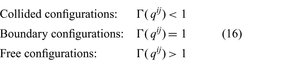
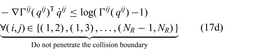
To avoid collisions between the joints of the arms, we need to devise a control algorithm to ensure that none of the robots’ body parts collide with each other. To achieve this objective, the IK solver must consider not only the kinematic constraints of each robot, but also self-collision constraints. Given that the robots’ bases are fixed with respect to each other, we can explore the joint workspace of the robots, in order to model the regions that may lead to collision. Since the space of joint configurations is continuous, we must approximate the regions of collisions by building a continuous map of the feasible (safe) and infeasible (collided) configurations. Assuming that the infeasible regions can be bounded through a continuous and continuously differentiable function $\mathrm{\Gamma }(q^{ij}):{\mathrm{ℝ}}^{d_{q_i}+d_{q_j}}\to \mathrm{ℝ}$ , where $q^{ij}=[q^i,q^j{]}^{\mathrm{T}}\in {\mathrm{ℝ}}^{d_{q_i}+d_{q_j}}$ are the joint angles of the $i$ th and $j$ th robots, respectively. We define $\mathrm{\Gamma }(.)$ such that

$$\begin{array}{ll}\mathrm{Collided\; configurations}:\hfill & \mathrm{\Gamma }(q^{ij})<1\hfill \\ \mathrm{Boundary\; configurations}:\hfill & \mathrm{\Gamma }(q^{ij})=1\hfill \\ \mathrm{Free\; configurations}:\hfill & \mathrm{\Gamma }(q^{ij})>1\hfill \end{array}$$

(16)

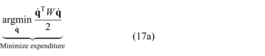
A data-driven approach for building $\mathrm{\Gamma }(q^{ij})$ is proposed in Section 5. Figure 5 illustrates a $\mathrm{\Gamma }(.)$ for a toy two-dimensional example. Equation (16) provides constraints that must be taken into account when solving the IK problem. We propose the following quadratic program to solve the IK:

$$\begin{array}{l}\underset{\mathrm{Minimize\; expenditure}}{\underbrace{\underset{\stackrel{.}{\mathbf{q}}}{\mathrm{argmin}}\frac{{\stackrel{.}{q}}^{\mathrm{T}}W\stackrel{.}{\mathbf{q}}}{2}}}\hfill \end{array}$$

(17a)

Subject to:

$$\begin{array}{l}\underset{\mathrm{Satisfy\; the\; desired\; end}-\mathrm{effector\; motion}}{\underbrace{\mathbf{J}(\mathbf{q})\stackrel{.}{\mathbf{q}}={\stackrel{.}{\mathbf{\xi }}}^R}}\hfill \end{array}$$

(17b)

$$\begin{array}{l}\underset{\mathrm{Satisfy\; the\; kinematic\; constraints}}{\underbrace{{\stackrel{.}{\mathit{\theta }}}^{-}\le \stackrel{.}{\mathbf{q}}\le {\stackrel{.}{\mathit{\theta }}}^{+}}}\hfill \end{array}$$

(17c)

$$\begin{array}{l}-\nabla {\mathrm{\Gamma }}^{ij}{(q^{ij})}^{\mathrm{T}}{\stackrel{.}{q}}^{ij}\le \log ({\mathrm{\Gamma }}^{ij}(q^{ij})-1)\hfill \\ \underset{\mathrm{Do\; not\; penetrate\; the\; collision\; boundary}}{\underbrace{\forall (i,j)\in \{(1,2),(1,3),\dots ,(N_R-1,N_R)\}}}\hfill \end{array}$$

(17d)

where $q=[q^1,\dots ,q^{N_R}{]}^{\mathrm{T}}\in {\mathrm{ℝ}}^{d_q}$ , $d_q={\displaystyle \sum _{i=1}^{N_R}}{d}_{q_i}$ . ⁴ Here $W$ is a block diagonal matrix of positive-definite matrices, $J=diag(J_1,\dots ,J_{N_R})$ is a block diagonal matrix of the Jacobian matrices, ${\stackrel{.}{\xi }}^R={\left[\begin{array}{ccc}{\stackrel{.}{\xi }}_1^R\hfill & \dots \hfill & {\stackrel{.}{\xi }}_{N_R}^R\hfill \end{array}\right]}^{\mathrm{T}}\in {\mathrm{ℝ}}^{d_n}$ , and $d_n=N_R{d}_n$ is the desired velocity given by (2). Here ${\stackrel{.}{\theta }}^i=\left[\begin{array}{ccc}{\stackrel{.}{\theta }}_1^i\hfill & \dots \hfill & {\stackrel{.}{\theta }}_{N_R}^i\hfill \end{array}\right]\forall i\in \{-,+\}$ and ${\stackrel{.}{\theta }}_i^{+}\in {\mathrm{ℝ}}^m$ and ${\stackrel{.}{\theta }}_i^{-}\in {\mathrm{ℝ}}^m$ are conservative lower and upper bounds of the joint limits, respectively. To integrate the joint limits into the velocity-level constraints, Xia and Wang (2000) proposed the following equation:

$$\begin{array}{l}{\stackrel{.}{\theta }}_i^{-}:=\max (\mu (q_i^{-}-q_i),{\stackrel{.}{q}}_i^{-})\hfill \\ {\stackrel{.}{\theta }}_i^{+}:=\min (\mu (q_i^{+}-q_i),{\stackrel{.}{q}}_i^{+})\hfill \end{array}$$

(18)

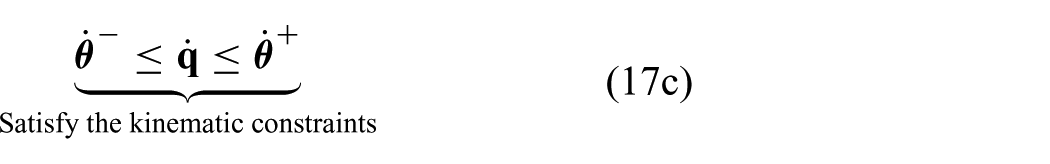
with $q_i^{-},q_i^{+},q_i^{-},{\stackrel{.}{q}}^{-}$ as the conservative lower and upper bounds on the joints’ positions and velocities. The intensity coefficients, $0<{\mu }_p$ , determine the magnitude of decelerations. This should be defined such that the feasible region of $\stackrel{.}{\theta }$ is greater than the joint velocity limits.

Fig. 5.

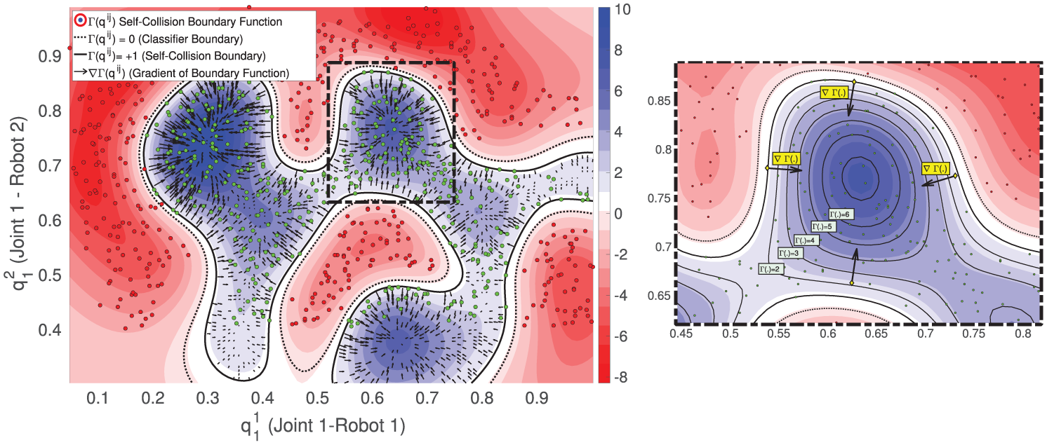
The $\mathrm{\Gamma }(q^{ij})$ function for a toy two-dimensional example. Assume there are two robots with 1 DOF each corresponding to each axis, i.e. $q^{ij}=[q_1^1,q_2^1]$ . The green data points represent “collision-free” robot configurations ( $y=+1$ ), while the red data points represent “collided” robot configurations ( $y=-1$ ). The background colors represent the values of $\mathrm{\Gamma }(q^{ij})$ ; refer to the colorbar for exact values, where the blue area corresponds to collision-free robot configurations ( $\mathrm{\Gamma }(q^{ij})>1$ ), the red area to collided configurations ( $\mathrm{\Gamma }(q^{ij})<1$ ). The arrows inside the collision-free region denote $\nabla \mathrm{\Gamma }(q^{ij})$ . We can see how $\nabla \mathrm{\Gamma }(q^{ij})$ pushes the robot configurations away from the self-collision boundary.

While the robots are far from the boundary configurations, the value of $\log ({\mathrm{\Gamma }}^{ij}(q^{ij})-1)$ is positive which relaxes the inequality constraints, i.e. the robots accurately follow the desired end-effector trajectory. When they are near the boundary configurations, the value of $\log ({\mathrm{\Gamma }}^{ij}(q^{ij})-1)$ is negative. Therefore, constraint (17d) forces the joint angles to move away from the boundary as they approach it. Since satisfying the collision avoidance and the kinematic constraints is of higher priority than following the desired end-effector motion, we give higher penalty to (17c) and (17d), than to (17b). In a particular case, when the robots are initiated inside of the boundary (i.e. ${\mathrm{\Gamma }}^{ij}(.)<1$ ), $\log ({\mathrm{\Gamma }}^{ij}(.)-1)$ is not defined. In this case, we replace $\log (\mathrm{\Gamma }(.)-1)$ with a large negative number that pushes the robots outward towards the boundary.

Equation (17) is a convex QP problem with equality and inequality constraints, hence, there is no closed-form solution for it. As the solutions to such linear optimization are solver-dependent, in terms of computation cost, we compare three approaches to solve (17). The first approach formulates (17) as a system of piecewise-linear equations and uses a DS-based approach to solve them (Xia and Wang, 2000; Zhang, 2005; Zhang et al., 2004). The second approach uses Nlopt, a standard non-linear programming solver (Johnson, 2016). The third approach uses a solver specifically designed for constrained convex problems; the solver that we use is called CVXGEN, introduced in (Mattingley and Boyd, 2012), which generates C codes, tailored for the specific formulation of (17). As the second and third approaches are ready to use interfaces, in the rest of this section we introduce the first approach. ⁵

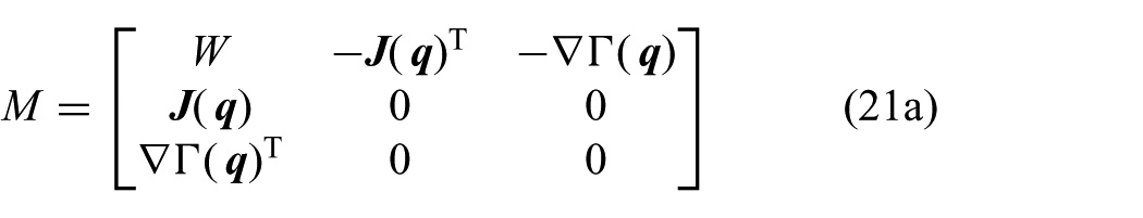
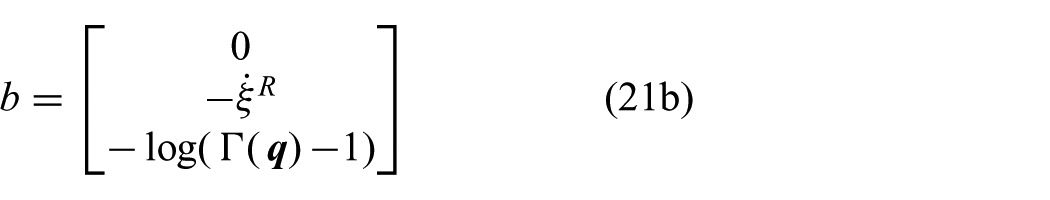
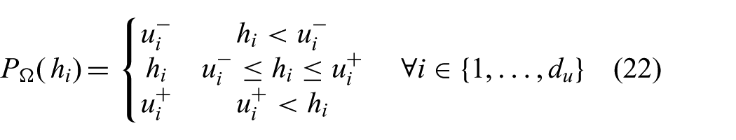
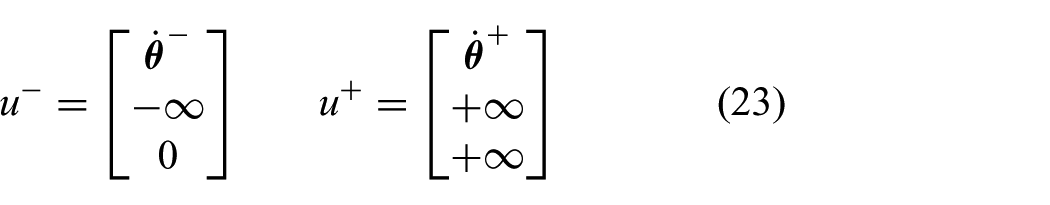
Lemma 1. Linear QP (17) is equivalent to the following system of piecewise-linear equations.

$$P_{\mathrm{\Omega }}(u-(Mu+b))-u=0$$

(19)

Moreover, the following DS is asymptotically stable to $u^{*}$ , where $u^{*}\in {\mathrm{ℝ}}^{d_u}$ is the solution of (19)

$$\stackrel{.}{u}=(I+M^{\mathrm{T}})(P_{\mathrm{\Omega }}(u-(Mu+b))-u)$$

(20)

where

$$M=\left[\begin{array}{ccc}W\hfill & -\mathit{J}{(\mathit{q})}^{\mathrm{T}}\hfill & -\nabla \mathrm{\Gamma }(\mathit{q})\hfill \\ \mathit{J}(\mathit{q})\hfill & 0\hfill & 0\hfill \\ \nabla \mathrm{\Gamma }{(\mathit{q})}^{\mathrm{T}}\hfill & 0\hfill & 0\hfill \end{array}\right]$$

(21a)

$$b=\left[\begin{array}{c}0\hfill \\ -{\stackrel{.}{\xi }}^R\hfill \\ -\log (\mathrm{\Gamma }(\mathit{q})-1)\hfill \end{array}\right]$$

(21b)

$u={\left[\begin{array}{ccc}\stackrel{.}{\mathit{q}}\hfill & \eta \hfill & \nu \hfill \end{array}\right]}^{\mathrm{T}}\in {\mathrm{ℝ}}^{d_u}$ , and $d_u=d_q+d_n+1$ . As $0\preccurlyeq W$ , $M$ is also positive semi-definite. Here $\eta \in {\mathrm{ℝ}}^{d_N}$ and $\nu \in \mathrm{ℝ}$ are the dual decision vectors and $P_{\mathrm{\Omega }}(h)=\left[\begin{array}{ccc}{P}_{\mathrm{\Omega }}(h_1)\hfill & \dots \hfill & P_{\mathrm{\Omega }}(h_{d_u})\hfill \end{array}\right]$ is the element-wise $\mathrm{\Omega }$ -projection operator defined as

$$P_{\mathrm{\Omega }}(h_i)=\{\begin{array}{cc}{u}_i^{-}\hfill & h_i<u_i^{-}\hfill \\ h_i\hfill & u_i^{-}\le h_i\le u_i^{+}\hfill \\ u_i^{+}\hfill & u_i^{+}<h_i\hfill \end{array}\forall i\in \{1,\dots ,d_u\}$$

(22)

where $u^{+}$ and $u^{-}$ are the bounds of the primal-dual decision vector $u$ defined as

$$\begin{array}{ll}{u}^{-}=\left[\begin{array}{c}{\stackrel{.}{\mathit{\theta }}}^{-}\hfill \\ -\infty \hfill \\ 0\hfill \end{array}\right]\hfill & u^{+}=\left[\begin{array}{c}{\stackrel{.}{\mathit{\theta }}}^{+}\hfill \\ +\infty \hfill \\ +\infty \hfill \end{array}\right]\hfill \end{array}$$

(23)

and $\mathrm{\Omega }=\{u\in {\mathrm{ℝ}}^{d_u}|u^{-}\le u\le u^{+}\}$ .

Proof. Refer to Zhang (2005) and Xia and Wang (2000).

Theorem 3. By taking $u$ and $(I+M^{\mathrm{T}})P_{\mathrm{\Omega }}(u-(Mu+b))$ as the output and the input of the system (20), respectively, Equation (20) is passive.

Proof. See Appendix F.

Remark 2. Theorems 1, 2 and 3 show that all the proposed DSs are passive. Hence, if the robots and the low level torque controllers are passive, the proposed framework for coordinated multi-arm system is passive and stable as it is a feedback system of passive elements.

The C++ implementation of the proposed centralized IK solver is provided by authors in QP_IK_solver, see Table 2.

5. Learning a SCA boundary

In this section, we introduce a data-driven approach to approximate the SCA boundary function $\mathrm{\Gamma }(q^{ij})$ , used in (17) as a constraint for the IK solver. As per (16), $\mathrm{\Gamma }(q^{ij})$ should be of class ${\mathcal{C}}^0$ and ${\mathcal{C}}^1$ and, interestingly, can be formulated as a binary classification problem, $y\leftarrow \mathrm{sgn}\left(\mathrm{\Gamma }(q^{ij})\right)$ for $y\in \{+1,-1\}$ , where “collided” joint configurations belong to the negative class (i.e. $y=-1$ ) and “non-collided” configurations belong to the positive class (i.e. $y=+1$ ). When $\mathrm{\Gamma }(q^{ij})=1$ , $q^{ij}$ is at the boundary of the positive class, i.e. the self-collision boundary (Figure 5).

To recall, the configuration space of a multi-arm system is an $n$ -dimensional torus $\left(S^1\times S^1\times \dots \times S^1(n-times)={\mathcal{T}}^N\right)$ for $n$ DOFs (LaValle, 2006). Given two robots with 7 DOFs each, the manifold in which the multi-arm joint-angle vector lies in is $q^{ij}\in {\mathcal{T}}^{14}$ . Employing $q^{ij}$ as the feature vector for a classification problem can be problematic for several reasons. First, many machine learning algorithms rely on computing distances/norms in Euclidean space, assuming the features are independent and identically distributed from an underlying distribution in ${\mathrm{ℝ}}^N$ . Hence, a Euclidean norm applied on $q^{ij}\in {\mathcal{T}}^N$ , is merely an approximation of the actual distance in the ${\mathcal{T}}^N$ manifold. In fact, a proper distance metric for joint-angles, i.e. $d(q_1^{ij},q_2^{ij})$ where $q^{ij}\in {\mathcal{T}}^N$ , is non-existent. For this reason, most trajectory optimization planning algorithms rely on mapping joint-space configurations to task space via forward kinematics (Holladay and Srinivasa, 2016; Stilman, 2007), where distances are well established.

Nevertheless, in kernel methods such as SVM (Scholkopf and Smola, 2001), one can overlook the topology of the input data and instead lift it onto a higher-dimensional feature space $\mathrm{\Phi }:{\mathrm{ℝ}}^N\to {\mathrm{ℝ}}^F$ , where the kernel trick, $k(x,x\prime )=〈\mathrm{\Phi }(x),\mathrm{\Phi }(x\prime )〉$ for $x\in {\mathrm{ℝ}}^N$ , is employed to find a separating hyperplane in the $F$ -dimensional feature space. Neural networks (NNs) can also alleviate the need for proper representations of the topology of the input space, as they are capable of learning highly complex and non-linear decision boundaries via soft sigmoid functions (Rojas, 1996). However, employing such methods directly on $q^{ij}$ comes at a cost, as the trade-off between model complexity and classification error would be hindered ⁶ .

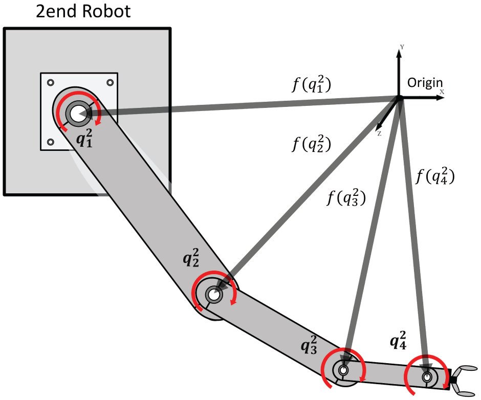
For such reasons, and in line with the trajectory optimization literature, instead of learning our SCA decision boundary function $\mathrm{\Gamma }(.)$ on the joint-angle data $q^{ij}$ , we learn $\mathrm{\Gamma }(.)$ on the three-dimensional Cartesian representation of the joint angles $f(q^{ij})$ . As illustrated in Figure 6, $f(q^{ij})$ is a vector composed of the three-dimensional Cartesian positions of all joints for the $i$ th and $j$ th robot, computed via forward kinematics. The feature vector for a dual-arm robotic system is, thus, $f(q^{ij})\in {\mathrm{ℝ}}^{3d_{q_i}+3d_{q_j}}$ . We posit that, by using $f(q^{ij})$ instead of $q^{ij}$ , we can achieve a better trade-off between model complexity and error rate. Moreover, since the output of $\mathrm{\Gamma }(.)$ is expected to be a scalar (16), no extra computation is necessary, as $\mathrm{\Gamma }(q^{ij})\equiv \mathrm{\Gamma }(f(q^{ij}))$ . The linear inequality constraints in (17d) require $\nabla \mathrm{\Gamma }(.)$ to be $\mathcal{C}$ , this can also be provided by either SVMs or NNs.

Fig. 6.

Illustration of $f(q^2)$ , three-dimensional Cartesian positions (e.g. $f(q_1^2):S^1\to {\mathrm{ℝ}}^3$ ) of the individual joint angles in the multi-arm system reference frame used to learn the SCA boundary function $\mathrm{\Gamma }(f(q^2))$ , where $f(q^2)=\{f(q_1^2),\dots ,f(q_2^4)\}$ , assuming we have two robots with 4 DOFs each.

In this work, we favor the use of SVMs, for two main reasons. (i) Learning a SVM is a convex optimization problem; hence, we can always reach a global optimum, whereas NNs rely on heavy parameter tuning and multiple initializations in order to avoid local minimum solutions. (ii) SVMs yield sparser models than NNs for high-dimensional non-linear classification problems, leading to better runtimes at the prediction stage. In the following sub-sections, we describe how we learn $\mathrm{\Gamma }(f(q^{ij}))$ through the SVM formulation from a simulated data set of “collided” and “non-collided” robot configurations. We present our method for constructing such a data set, motivate and propose to use a sparse SVM learning algorithm (Joachims and Yu, 2009) to achieve runtime limitations imposed by the robot control loop, as discussed later on.

5.1. ${\mathcal{C}}^0$ and ${\mathcal{C}}^1$ SCA boundary via SVM

We follow the kernel SVM formulation and propose to encode $\mathrm{\Gamma }\left(f(q^{ij})\right)$ as the SVM decision rule. By omitting the sign function and using the radial basis function (RBF) kernel $k\left(f(q^{ij}),f(q_n^{ij})\right)=e^{\left(-\frac{1}{2{\sigma }^2}||f(q^{ij})-f(q_n^{ij}{)||}^2\right)}$ , for a kernel width $\sigma$ ; $\mathrm{\Gamma }\left(f(q^{ij})\right)$ has the following form, ⁷

$$\begin{array}{c}\mathrm{\Gamma }\left(f(q^{ij})\right)={\displaystyle \sum _{n=1}^{N_{sv}}}{\alpha }_n{y}_{n}k\left(f(q^{ij}),f(q_n^{ij})\right)+b\hfill \\ ={\displaystyle \sum _{n=1}^{N_{sv}}}{\alpha }_n{y}_n{e}^{\left(-\frac{1}{2{\sigma }^2}||f(q^{ij})-f(q_n^{ij}{)||}^2\right)}+b\hfill \end{array}$$

(24)

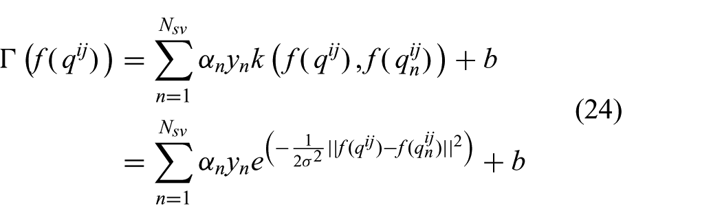
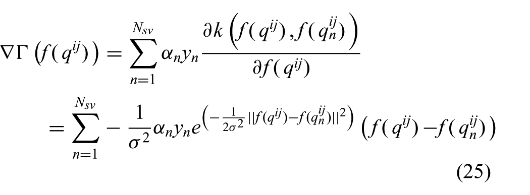
for $N_{sv}$ support vectors, where $y_i\in \{-1,+1\}$ are the positive/negative labels corresponding to non-collided/collided configurations, $0\le {\alpha }_i\le C$ are the weights for the support vectors that must yield ${\displaystyle {\sum }_{n=1}^{N_{sv}}}{\alpha }_n{y}_n=0$ and $b\in \mathrm{ℝ}$ is the bias for the decision rule. Here $C\in \mathrm{ℝ}$ is a penalty factor used to trade-off between maximizing the margin and minimizing classification errors. Given $C$ and $\sigma$ , ${\alpha }_i$ and $b$ are estimated by solving the dual optimization problem for the soft-margin kernel SVM (Scholkopf and Smola, 2001). Moreover, Equation (24) naturally yields a continuous gradient as follows,

$$\begin{array}{c}\nabla \mathrm{\Gamma }\left(f(q^{ij})\right)={\displaystyle \sum _{n=1}^{N_{sv}}}{\alpha }_n{y}_n\frac{\partial k\left(f(q^{ij}),f(q_n^{ij})\right)}{\partial f(q^{ij})}\hfill \\ ={\displaystyle \sum _{n=1}^{N_{sv}}}-\frac{1}{{\sigma }^2}{\alpha }_n{y}_n{e}^{\left(-\frac{1}{2{\sigma }^2}\left|\right|f(q^{ij})-f(q_n^{ij}{)||}^2\right)}\left(f(q^{ij})-f(q_n^{ij})\right)\hfill \end{array}$$

(25)

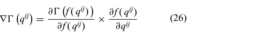
Although $\nabla \mathrm{\Gamma }(f(q^{ij}))$ already satisfies the constraints imposed by (17d), it lives in a $3d_{q_i}+3d_{q_j}$ -dimensional space, $\nabla \mathrm{\Gamma }\left(f(q^{ij})\right)\in {\mathrm{ℝ}}^{3d_{q_i}+3d_{q_j}}$ . We must then project this gradient onto its corresponding ${\mathrm{ℝ}}^{d_{q_i}+d_{q_j}}$ joint space, i.e. $\nabla \mathrm{\Gamma }(q^{ij})\in {\mathrm{ℝ}}^{d_{q_i}+d_{q_j}}$ with the following expansion:

$$\begin{array}{l}\nabla \mathrm{\Gamma }\left(q^{ij}\right)=\frac{\partial \mathrm{\Gamma }\left(f(q^{ij})\right)}{\partial f(q^{ij})}\times \frac{\partial f(q^{ij})}{\partial q^{ij}}\hfill \end{array}$$

(26)

the first term is equivalent to (25) and the second term is, in fact, the Jacobian of each three-dimensional joint position with respect to each joint angle $J(q^{ij})=\frac{\partial f(q^{ij})}{\partial q^{ij}}$ for which we have a closed-form solution.

5.2. SCA data set construction

In order to learn $\mathrm{\Gamma }(f(q^{ij}))$ , we must initially generate a data set capable of identifying the so-called self-collision boundary. We begin by describing our simplified geometric representation of the robot’s kinematic configuration used to identify “collided” and “non-collided” configurations.

For simplicity, let us assume a dual-arm setting, with each arm being a KUKA 7-DOF arm (Figure 8). Similar to Zucker et al. (2013), we simplify the representation of the robot’s structure by fitting spheres to each joint and its adjoining physical structure as shown in Figure 7. By doing so, we generate a discrete representation of the multi-arm robotic system as a set of spheres $S^{ij}=\{s_1^i,\dots ,s_7^i,s_1^j,\dots ,s_7^j\}$ . By using spheres as a geometric representation of a joint, we simplify the distance computation between joints, as the distance from any point in a sphere to the nearest obstacle is lower-bounded to $d(c)-r$ , where $c$ is the center of the sphere and $r$ its corresponding radius (Ratliff et al., 2009). Further, the lower-bound between two spheres is the distance between their centers ( $c_k^i$ ) minus the sum of their respective radii ( $r_k^i$ ), for the $k$ th spheres of the $i$ th robot. For example, given $s_5^1$ and $s_7^2$ the lower-bounded distance between them can be computed as $d(s_5^1,s_7^2)=d(c_5^1,c_7^2)-(r_5^1+r_7^2)$ .

Fig. 7.

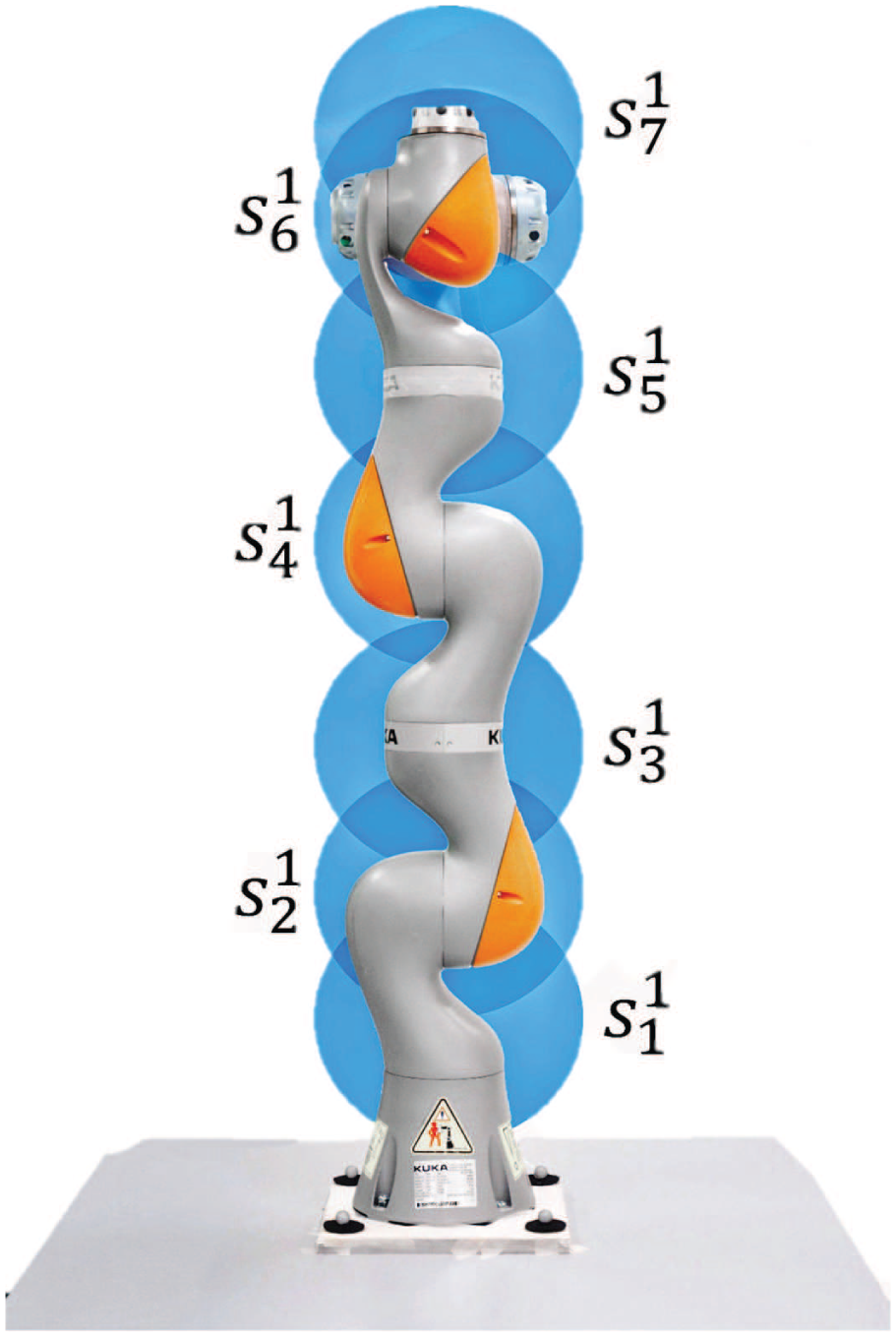
Illustration of $S^1=\{s_1^1,\dots ,s_7^1\}$ for a KUKA IIWA 7-DOF robot arm. Here $S^i$ is the geometric representation of the $i$ th robot with a set of spheres corresponding to each joint used to construct the SCA data set. If a tool is attached to the arm, the last sphere is enlarged such that it encapsulates its extremities.

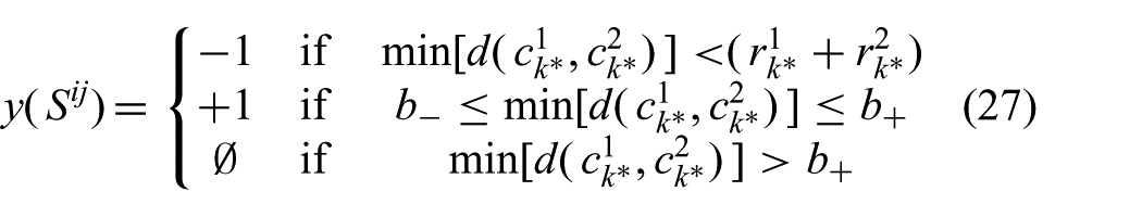
To identify collision in the dual-arm system, we compute the pairwise distances of the centers of the set of spheres of the $i$ th robot ( $S^i$ ) with respect to the set of spheres of the $j$ th robot ( $S^j$ ) and find the minimum distance $\min [d(c_{k^{*}}^1,c_{k^{*}}^2)]$ . We then define a label for each robot configuration $S^{ij}$ as follows,

$$y(S^{ij})=\{\begin{array}{ccc}-1\hfill & \mathrm{if}\hfill & \min [d(c_{k^{*}}^1,c_{k^{*}}^2)]<(r_{k^{*}}^1+r_{k^{*}}^2)\hfill \\ +1\hfill & \mathrm{if}\hfill & b_{-}\le \min [d(c_{k^{*}}^1,c_{k^{*}}^2)]\le b_{+}\hfill \\ \varnothing \hfill & \mathrm{if}\hfill & \min [d(c_{k^{*}}^1,c_{k^{*}}^2)]>b_{+}\hfill \end{array}$$

(27)

where $r_{k^{*}}^i$ corresponds to the radius of the $k$ th sphere, and $b_{-}$ , $b_{+}$ correspond to minimum/maximum distances of the “safe” boundary. Specifically, a joint configuration is “collided,” i.e. labeled as $y=-1$ , when the $\min [d(c_{k^{*}}^1,c_{k^{*}}^2)]$ between the centers of the closest spheres is less than the sum of the radii of the corresponding spheres, i.e. $(r_{k^{*}}^1+r_{k^{*}}^2)$ . In practice, we set the spheres to a fixed radius of $10cm$ , hence $(r_{k^{*}}^1+r_{k^{*}}^2)=20$ cm. Given that virtually any robot configuration where $\min [d(c_{k^{*}}^1,c_{k^{*}}^2)]>(r_{k^{*}}^1+r_{k^{*}}^2)$ can be considered “non-collided” configurations, we would end up with a heavily un-balanced data set of “collided”/“non-collided” data points. We thus introduce a decomposition of the “non-collided” robot configurations into “boundary”, labeled as $y=+1$ , and “safe” configurations, which are not labeled $y=\varnothing$ . If $\min [d(c_{k^{*}}^1,c_{k^{*}}^2)]$ lies within a safety margin, denoted by $b_{-}$ and $b_{+}$ , the robots are very close to each other but still safe, see Figure 8. We empirically found $b_{-}=30$ cm and $b_{+}=33$ cm to be safe boundaries for our dual-arm setting. Hence, a “non-collided” configuration is in fact a “boundary” configuration, as all of the “safe” configurations are filtered out. This has a geometric meaning, rather than finding the margin between “collided” and “safe” configurations, our boundary function will model the tighter margin between “non-collided” and “boundary” configurations. From herein, we consider “boundary” configurations as the “non-collided” configurations.

Fig. 8.

Examples of the collided/boundary configurations of a dual-arm setting with an offset of $X_{off}=[0.0,1.3.0.34]$ m between their bases (visualized in the RVIZ simulation environment; see http://wiki.ros.org/rviz). (b), (d) and (f) are examples of the boundary configurations and (c), (e) and (g) are examples of the collided configurations.

To generate the positive ( $y(S^{ij})=+1$ ) and negative samples ( $y(S^{ij})=-1$ ) for our SCA data set, we sample from all the possible motions of the robots in their respective workspaces and apply (27) to each configuration. To explore all possible joint configurations $q^{ij}$ , we systematically displace all of the joints of both robots by $20\mathrm{deg}$ each. Joints $q_1^i$ , $q_3^i$ , $q_5^i$ , and $q_7^i$ have a range of $\pm 170\mathrm{deg}$ , whereas joints $q_2^i$ , $q_4^i$ , and $q_6^i$ have a range of $\pm 120\mathrm{deg}$ . Given the $20\mathrm{deg}$ sampling resolution, this leads to $18$ samples for the former group and $13$ for the latter. One can see from Figure 7 that sampling joint $q_7^i$ has no effect on the configuration of the spheres (even when considering a tool attached to it). Hence, the total number of possible configurations is ${18}^3{*12}^3$ . C++ code to efficiently generate such data set is provide in the SCA_boundary_construction package (Table 2), the user needs only to specify the $X_{off}$ between robot bases and the DH parameters of each arm. For our dual-arm setting we gathered a data set of approximately $\approx 5.4$ million data points, $\approx 2.4$ million belonging to the “collided” configuration class $y=-1$ and the rest to the “non-collided” configurations $y=+1$ . Owing to our systematic sampling of “collided” and “boundary” robot configurations, we can generate such balanced data sets, which is desirable for any learning algorithm.

5.3. Efficient SVMs for large data sets

The training time of a kernel SVM has a complexity of $\approx \mathcal{O}({N_M}^{2}D)$ , where $N_M$ is the number of samples and $D$ is the dimension of the data points. Prediction time, on the other hand, depends on the number of support vectors $N_{sv}$ learned through training. In practice, the $N_{sv}$ tends to increase linearly with the amount of training data $N_M$ (Bakir et al., 2004). More specifically, for a kernel SVM $N_{sv}/N_M\to {ℬ}_k$ , where ${ℬ}_k$ is the smallest achievable classification error by the kernel $k$ (Steinwart, 2003), i.e. in a non-separable classification scenario, to achieve $5\%$ error, at least $5\%$ of the training points must become support vectors. This comes as a nuisance when large training sets are involved, as is the case for our application. A $N_{sv}\gg$ signifies a dense solution for representing the hyper-plane of the classifier margin $w={\displaystyle {\sum }_{i=1}^{N_{sv}}}{\alpha }_i{y}_i\mathrm{\Phi }(f(q_i^{ij}))$ . Naturally, the denser the solutions, the more computationally expensive they are at run-time. This makes dense SVMs infeasible for real-time robot control. In order to achieve fast adaptation for both the desired end-effector positions and self-collisions, the IK solver must run (at most) at a rate of 2 ms. During this cycle, prior to solving (17), both (24) and (26) must be evaluated.

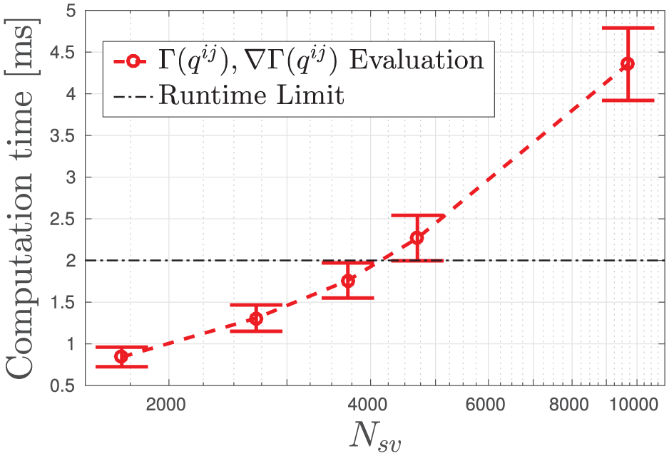
Given the desired control rate (2 ms), the specific hardware used to control the robots (i.e. 3.4 GHz i7 PC with 8 GB RAM) and the kinematic specifications of each robot, we can define a computational budget for our SCA boundary function. This budget translates to defining a limit of the maximum allowable $N_{sv}$ for our SVM representation of $\mathrm{\Gamma }(f(q^{ij}))$ . In Figure 9, we show a plot of different computation times ⁸ for the evaluation of (24) and (26) for the dual-arm setting shown in Figure 8. We omit computation time of the IK solver as this is presented in detail in Section 6 and Figure 17b. These computation times evaluate the implementation of $\mathrm{\Gamma }(f(q^{ij}))$ and $\nabla \mathrm{\Gamma }(f(q^{ij}))$ from the C++ SVMGrad (Table 2) package, provided by the authors.

Fig. 9.

Comparison of runtime computational cost for evaluating $\mathrm{\Gamma }(f(q^{ij}))$ and $\nabla \mathrm{\Gamma }\left(f(q^{ij})\right)$ on a Dell Optiplex 3.4 GHz i7 PC with 8 GB RAM for the dual-arm setting in Figure 6. The compared SVM models have the following increasing complexity $N_{sv}=\{1700,2700,3700,4700,9700\}$ . The presented runtimes are the mean and standard deviation of $\approx 2000\mathrm{H}z$ control loop cycles (equivalent to $\approx 4$ s) of the SCA test. The maximum allowable $N_{sv}$ in order to comply with the 2 ms runtime limit is $N_{sv}\le 3700$ , which can only be obtained by using $\le 1.5\%$ of this specific training data set. However, the IK solver takes $\approx 1$ ms to converge, hence, the actual limit would be around $N_{sv}\le 3000$ .

According to Figure 9, in order to comply with the 2 ms runtime requirement, we have a computational budget of $N_{sv}\le 3000$ . Given the size of our data set, it is not feasible to train SVM models that typically optimize for the dual through a variant of sequential minimal optimization (SMO) (Platt, 1999) or SMO-type decomposition methods (Bordes et al., 2005; Chang and Lin, 2011; Joachims, 1999). The fact that SVM learning algorithms tend to produce dense solutions has been recognized as one of its main weaknesses. To this end, several approaches have been proposed in order to solve the problem of finding sparser solutions to $w$ . These can be categorized into: (i) post-processing approximations and (ii) objective function or optimization strategy modification. The former approaches rely on approximating a sparse solution to an initially dense SVM (through the exact solution). The latter approaches either modify the SVM objective function by imposing sparsity constraints or propose a modified optimization algorithm for with sparsity considerations.

In this work, we choose one of the prevailing approaches that reformulates the SVM optimization problem, namely the cutting plane subspace pursuit (CPSP) method introduced by Joachims and Yu (2009), as it directly estimates a solution to the hyper-plane with a strict bound on the number of support vectors $k_{max}$ . A short motivation for selecting this method is discussed in Appendix H. In short, the CPSP method approximates a sparse hyper-plane by expressing it in terms of a set $B=\{b_1,\dots ,b_{k_{max}}\}$ of basis vectors $b_i\in {\mathrm{ℝ}}^{3d_{q_i}+3d_{q_j}}$ (not necessarily training points) as follows,

$$w={\displaystyle \sum _{i=1}^{k_{max}}}{\alpha }_i{y}_i\mathrm{\Phi }(b_i)$$

(28)

The optimization algorithm to estimate (28) then focuses on pursuing such a subspace through the fixed-point iteration approach for RBF kernels (Scholkopf and Smola, 2001). The learned basis vectors $B$ and ${\alpha }_i$ can be directly used in (24) and (25). We direct the interested reader to Joachims and Yu (2009) for theoretical equivalence proofs and implementation details of this learning approach.

Learning performance of $\mathrm{\Gamma }(f(q^{ij}))$

We begin our $\mathrm{\Gamma }(f(q^{ij}))$ learning performance analysis by presenting results from learning exact SVMs from small sub-samples of the 5.4 million point data set. To generate such comparison, the libSVM library (Chang and Lin, 2011) ⁹ was used for learning the SVM models, cross-validation was performed with routines from ML_toolbox ¹⁰ to find the optimal hyper-parameters. A $50\%$ split for training+validation/testing data sets was used to generate such evaluations. We evaluate five models with increasing complexity $N_{sv}=\{1700,2700,3700,4700,9700\}$ . These were learned from using $\{0.5\%,1\%,1.5\%,2\%,5\%\}$ of the training set (i.e. 2.7 million data points). ¹¹ For each model, a 10-fold cross-validation was performed to find the optimal hyper-parameters $C$ and $\sigma$ which yield the best trade-off between $N_{sv}/N_M$ and classification accuracy. The search space of each hyper-parameter was log-spaced in the following ranges $C{=[10}^{-1}{,10}^4]$ and $\sigma =[0.2,2]$ . ¹² In our application, we care about correctly classifying the negative class (i.e. “collided” configurations), for this we have two objectives.

• Minimize false positive rate (FPR): The $FPR=\frac{FP}{(FP+TN)}$ , otherwise known as fall-out error, quantifies the probability of negative samples ( $y=-1$ ) being classified as positive ( $y=+1$ ). This is equivalent to maximizing the true negative rate ( $TNR=1-FPR$ ). Classifying “collided” configurations ( $y=-1$ ) as “non-collided” configurations ( $y=+1$ ) yields a false positive ( $FP$ ). This error is critical as it would cause the IK solver to move the robots into an infeasible region, leading to collision and possibly permanent damage.

• Maximize true positive rate (TPR): The $TPR=\frac{TP}{(TP+FN)}$ , otherwise known as recall or sensitivity, quantifies the probability of positive samples ( $y=+1$ ) being classified as positive ( $y=+1$ ). This is equivalent to minimizing the false negative rate ( $FNR=1-TPR$ ). Classifying “collided” configurations ( $y=+1$ ) as “non-collided” ( $y=-1$ ) yields a false negative ( $FN$ ). This error is not as critical as the former, but it has an effect on the performance of the IK solver, as classifying “non-collided” configuration as “collided” would restrict the IK solver to move the robots into regions that are indeed feasible.

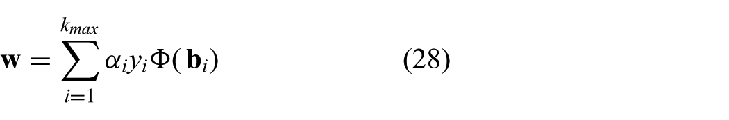
For reference, we also present accuracy $ACC=\frac{TP+TN}{(TP+FP+FN+TN)}$ and F1-score $F1=\frac{2TP}{(2TP+FP+FN)}$ . As can be seen from Figure 10, we can achieve optimal error rates on the testing set of $FPR\approx 1.3\%$ and $TPR\approx 97.54\%$ , with $5\%$ of the training data set, albeit surpassing the $N_{SV}$ limit. One might argue that, with such high performance of models trained on a minuscule amount of data (relative to the complete data set), perhaps such a large data set is not necessary. This is related to the SCA data set construction procedure (Section 5.2), where we set the joint sampling interval to $20\mathrm{deg}$ . An analysis of the performance of SVM models trained on data sets with lower sampling resolutions is provided in Appendix G. In short, as we increase the joint sampling resolution, less “collided” configurations are seen, resulting in drastic increases in $FPR$ .

Fig. 10.

Performance comparison of learning exact SVM models on randomly sub-sampled data sets versus sparse SVM models on larger chunks of the data set. Each model was evaluated on the test set, which contains 2.7 million unseen sample robot configurations. We present accuracy (ACC), F-1 Score (F1), false positive rate (plotted as 1-FPR), true positive rate (TPR), and $N_{sv}$ . Left: With the random sub-sampling method, using the second model ( $N_{sv}=2700$ ), one can achieve $FPR\approx 2.4\%$ and $TPR\approx 96.19\%$ within the desired 2 ms runtime limit. Right: With a sparse SVM model trained on 540000 points we can achieve $FPR\approx 1.45\%$ and $TPR\approx 97.4\%$ $k_{max}=3000$ .

From Figure 10, we can see that with the second model (i.e. $1\%$ of training data), we achieve error rates of: $FPR\approx 2.4\%$ and $TPR\approx 96.19\%$ within the computational budget. This is quite acceptable performance, however, due to the delicacy of our application we seek to achieve the best solution possible, i.e. at least $FPR\approx 1\%$ . In Figure 10, we present the results of using the CPSP SVM learning approach on different sub-sets of our training data limited to a support vector budget of $k_{max}=3000$ , specifically $\{2.5\%,5\%,10\%,20\%\}$ . As can be seen, for the models learned on data sets with the same size as the exact SVM solutions, the results are marginally lower. However, as the number of training points increases the error rates improve as much as $FPR=1.5\%$ and $TPR=97.4\%$ for a training set of 540,000 points. By using this sparse learning method we have proven that the optimal error rate can be achieved with minimal model complexity.

6. Empirical validation

The performance of the proposed framework is implemented on two different real dual-arm platforms. On the first platform, the coordination between the arms and with the object is evaluated. The second experimental set up is designed to evaluate the performance of dual-behavior and the self-collision avoidance.

6.1. First experimental set-up

The proposed framework is implemented on a real dual-arm platform, consisting of two 7-DOF robotic arms, namely a KUKA LWR 4+ and a KUKA IIWA mounted with a 4 -OF Barrett hand and a 16-DOF Allegro hand. As the results from the first set-up were presented in our previous work, we only summarize the main points. For more information, the readers are referred to Salehian et al. (2016a).

The empirical validation is divided into two parts that demonstrate the controller’s ability: (i) coordinate the multi-arm systems; (ii) rapidly adapt bi-manual coordination to intercept a flying object, without using a pre-defined model of the object’s dynamics. As the synchronized behavior is the only desired behavior in this section, the value of synchronization parameters are manually set to one.

6.1.1. Coordination capabilities

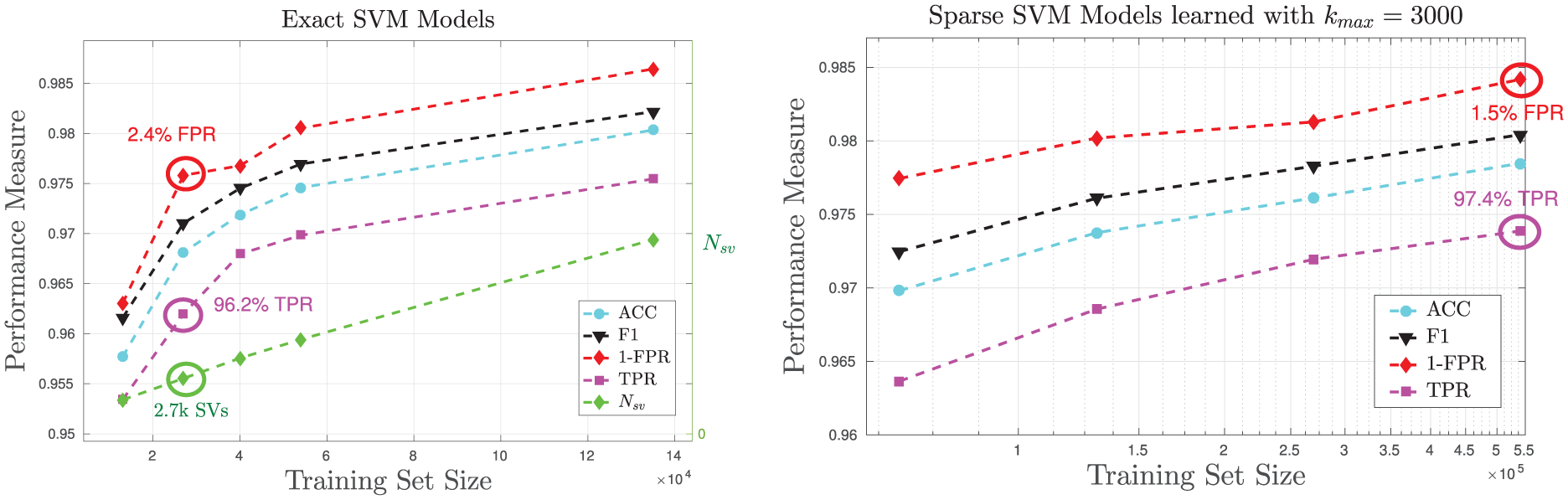
The first scenario is designed to illustrate the coordination capabilities of the arms with each other through the virtual object. As the human operator perturbs one of the robot arms, the virtual object is also perturbed, resulting in a stable synchronous motion of the other unperturbed arm (Figure 11). Since we offer a centralized controller based on the virtual object’s motion, there is no master/slave arm; thus, when any of the robots are perturbed, the others will synchronize their motions accordingly.

Fig. 11.

Snapshots of the video illustrating coordination of the arms in free space. Both arms are manually assigned to the synchronized behavior and as the object is outside the workspace of the robots, the coordination parameter $\gamma$ is close to zero. The human operator perturbs one of the arms, which leads the other arm to move in synchrony following the motion of the virtual object attached to the two end-effectors.

6.1.2. Reaching for fast flying objects

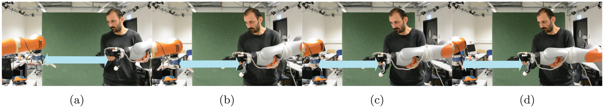
The second scenario is designed to show the coordination between the robots and a fast moving object, where a rod $(150cm\times 1cm)$ is thrown to the robots from 2.5 m away, resulting in approximately 0.56 s flying time. Due to inaccurate prediction of the object trajectory, the feasible intercept points need to be updated and redefined during the motion execution. The new feasible intercept point is chosen in the vicinity of the previous one to minimize the convergence time. As the motion of the object is fast and the predicted reaching points are not accurate, the initial values of $\gamma$ in (15) are set to $0.5$ . This decreases the convergence duration of the robots to the real object. Snapshots of the real robot experiments are shown in Figure 12. Visual inspection of the data and video confirmed that the robots coordinately follow the motion of the object and intercept it in the vicinity of the predicted feasible intercept point.

Fig. 12.

Snapshots of the arms reaching for a fast moving object. The object is specified by a blue square. The arms move in THE same direction (a) or in opposite directions (b) to keep the coordination between the arms and with the object. In order to not damage the robot’s hands, the robot hands do not close on the object when the hands intercept the object. A corresponding video for these experiments can be found in our previous publication (Salehian et al., 2016a).

6.2. Second experimental set-up

The proposed framework is implemented on a dual-arm platform, consisting of two 7-DOF KUKA IIWA robotic arms mounted with a two-finger Robotiq gripper and a 16-DOF Allegro hand. The robots are controlled via a fast research interface (FRI) in joint impedance mode. The fingers are controlled with joint angle position controllers in two states: open and close. ¹³ All the hardware involved (e.g. arms and hands) are controlled by one 3.4 GHz i7 PC. ¹⁴ The position of the feasible reaching points of the objects are captured by an Optitrack motion capture system from Natural point at $240$ Hz. As the outputs of the vision system are noisy, a Savitzky–Golay filter ¹⁵ is used to smooth the position of the object and estimate velocity and acceleration from these position measurements.

Our empirical validation is divided into two parts that demonstrate the controller’s capabilities: (i) estimation of the desired behavior and accordingly adaptation of the two arms’ motions; i.e. move independently or in coordination; (ii) SCA. A corresponding video is available at as Extension 1.

The performance of the framework is systematically assessed in three different levels to show: (i) the success rate of coordinately reaching for moving object; (ii) performance of IK solvers; and (iii) sensitivity of the framework to noise.

6.2.1. Dual-behavior capabilities

The first scenario is designed to illustrate the dual-behavior capabilities of the arms. The asynchronous behavior of each robot is to reach a fixed target (see Figure 13) or follow the hands of operator $1$ who stands between the arms (see Figure 14). The synchronized behavior is to coordinately reach an object brought by operator $2$ . A visual inspection of the data shows that when operator $2$ moves the object toward the robots, based on (8), the value of ${\tau }_{c_i}\forall i\in \{1,2\}$ smoothly increases to one. Hence, a smooth transition from the unsynchronized behavior to the synchronized behavior is achieved; see Figures 13 and 14. As there is no full coordination between the arms while the value of ${\tau }_{c_i}\forall i\in \{1,2\}$ is less than one, perturbing one arm does not affect the motion of other arm, see Figure 14(a)–(d). While the arms are allocated to the synchronized behavior, due to (15), the arms successfully track, coordinate with, and intercept the object and with each other, see Figure 14(g) and (h).

Fig. 13.

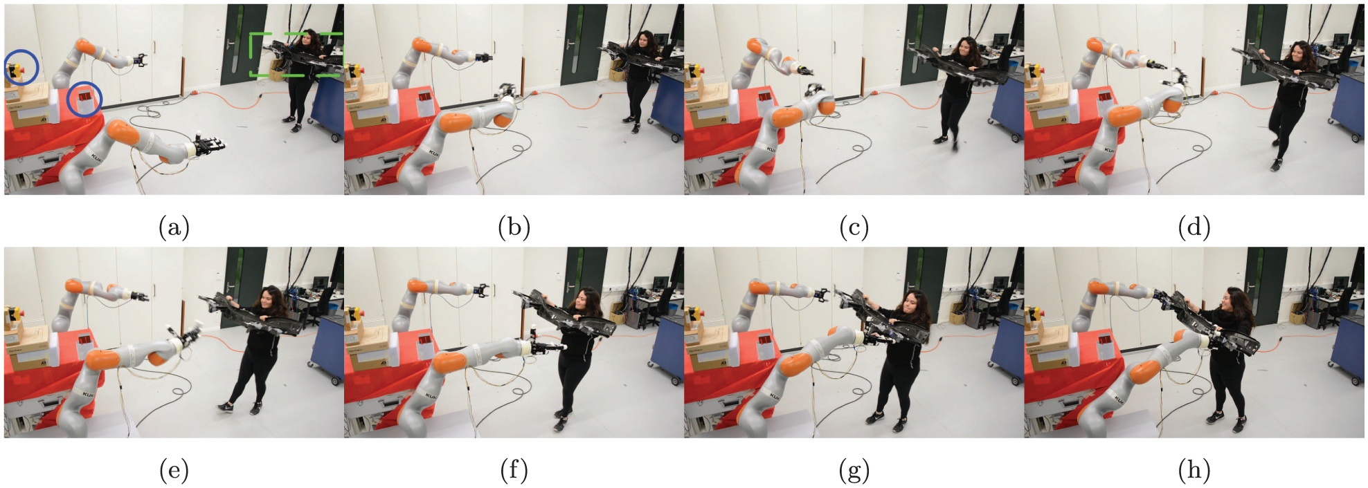
Snapshots of the video illustrating of dual behavior capabilities. The target of synchronous and asynchronous behaviors are highlighted in (a) by the green square and the blue circles, respectively. Initially, the robots are allocated to the asynchronous behavior. Hence, the robots moves toward the asynchronous targets in (b) and (c). In (d), ${\gamma }_{c_i}\approx 1\forall i\in \{1,2\}$ as the operator moves the object toward the arms, i.e. the synchronous behavior. Consequently, the robots coordinately and simultaneously reach and intercept the object at the desired reaching points.

Fig. 14.

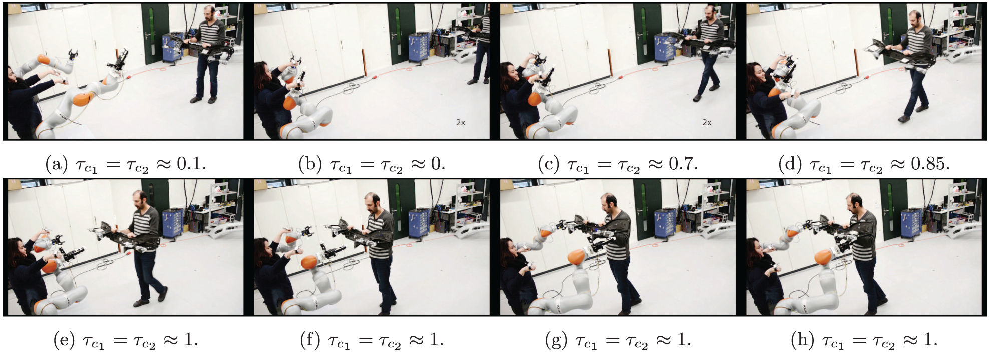
Snapshots of the video illustrating of dual behavior capabilities. The asynchronous behavior is to follow the hands of the operator $1$ who is inside of the robot workspaces. When the operator $2$ moves the object away from or toward the arms, the synchronization parameter smoothly goes to $0$ and $1$ , respectively.

6.2.2. SCA

Even though the SCA is successfully tested in all the experiments, we designed two different scenarios to highlight the performance of the IK solver with this constraint. As the motion of the fingers are not considered in the generated data set, see Section 5.2, we removed the hands in these two scenarios. In the first scenario, both robots move on straight lines to reach fixed and predefined targets. The targets are picked such that the arms surely collide with each other if the collision avoidance constraint is not considered. Figure 15c shows the initial and the final configurations. As it can been seen from Figures 15a the value of $\mathrm{\Gamma }(.)$ is coordinately updated during the motion execution with respect to the robot configurations and when it is less than two, based on (17d), the robots are moved away from each other to increase their distance. The minimum distance between the robots’ segments are shown in Figure 15b. In the second scenario, the end-effectors are following the hands of an operator. Visual inspection of the data and video confirmed that the robots follow the targets while any collision between them are avoided. A partial result of this experiment is presented in the accompanying video, see Extension 1.

Fig. 15.

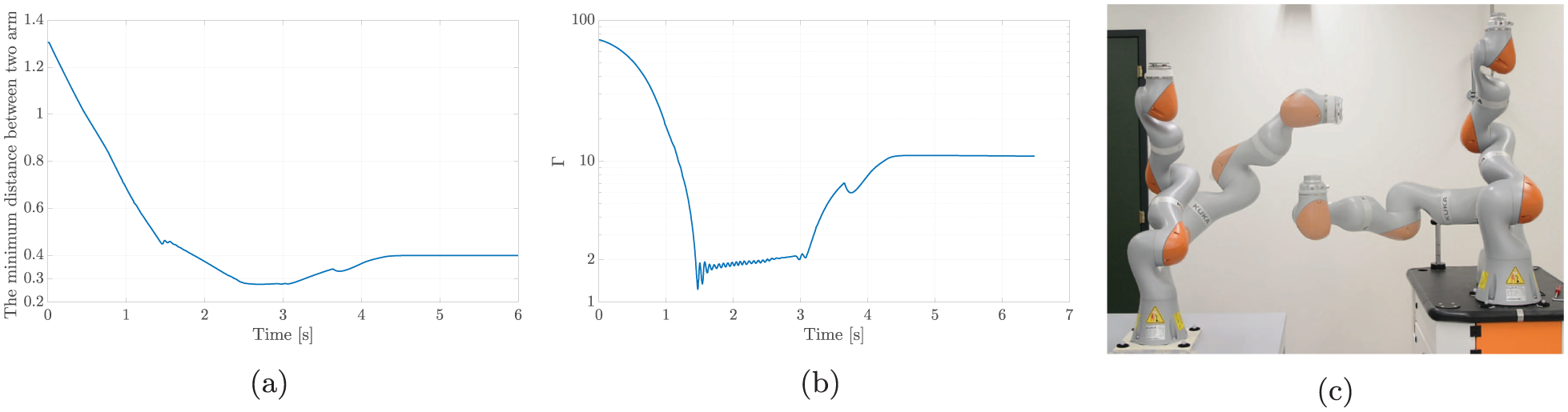
The distance between the bases of the arms are ${[0.0-1.30.14]}^{\mathrm{T}}$ m. The targets are ${[0.0-0.60.55]}^{\mathrm{T}}$ m, and ${[0.0-0.60.55]}^{\mathrm{T}}$ m for the arms of the left and right, respectively. In (a), the initial and the final configurations (transparent one) are depicted. In (b) and (c) the minimum distance between the arms and the value of $\mathrm{\Gamma }$ during the motion execution are shown. It can be shown that $\mathrm{\Gamma }$ never goes below $1$ , which indicates that the motion of the arms is safe.

6.2.3. Systematic assessment

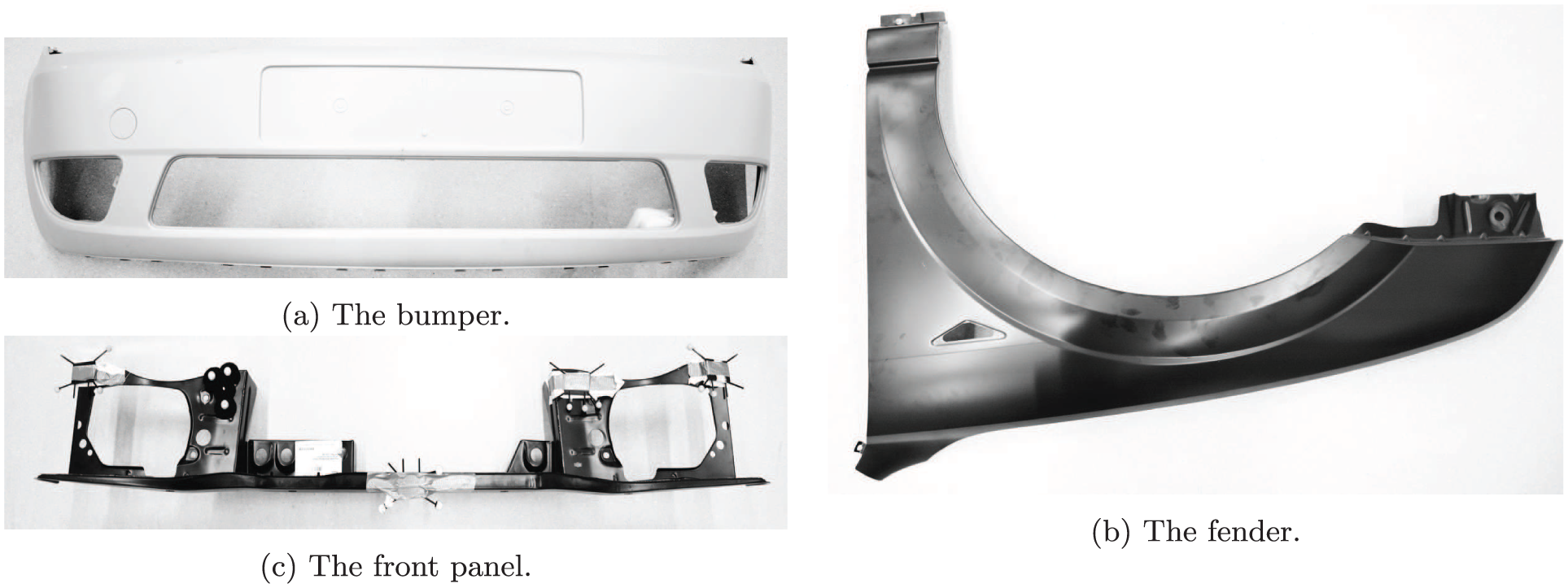
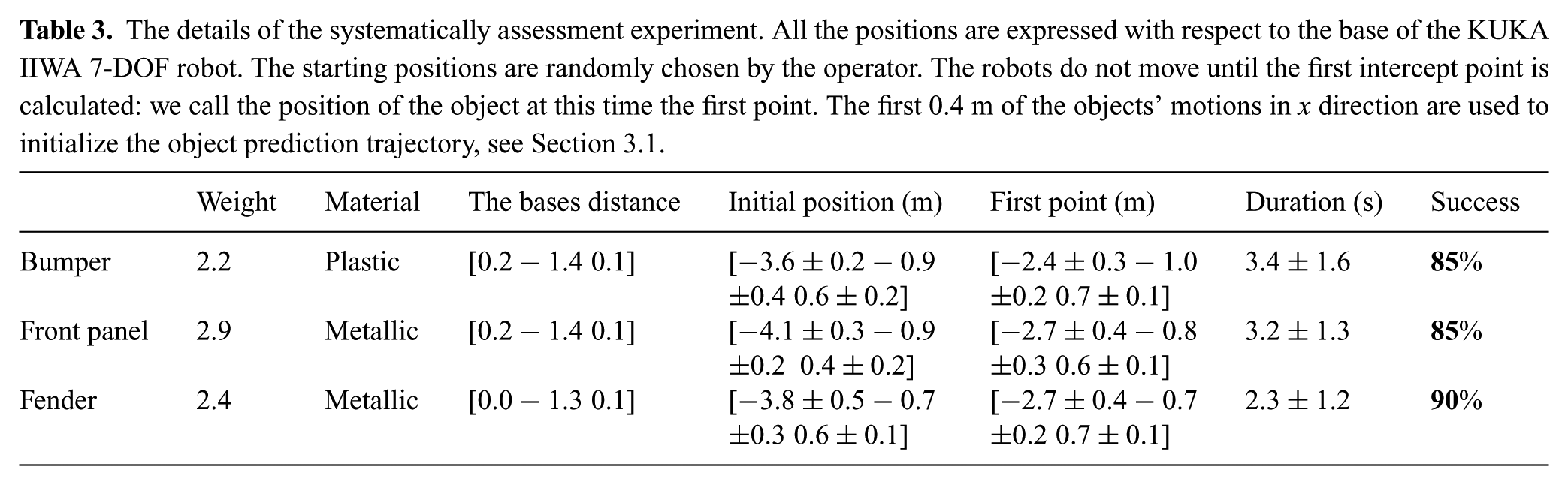
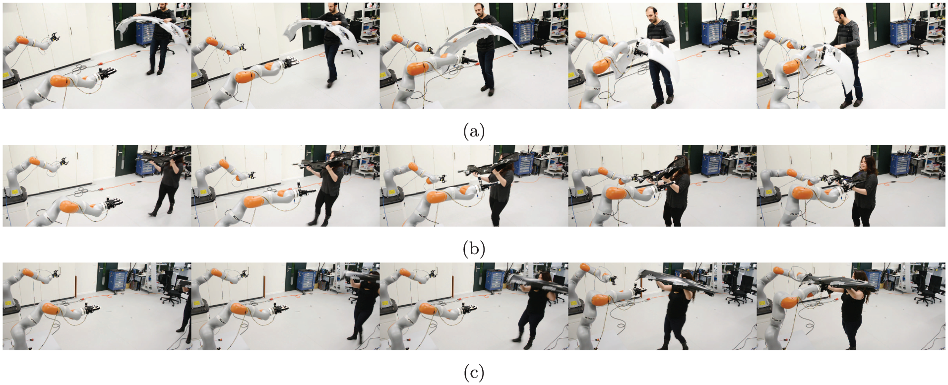
Coordination and adaptation assessment. To systematically assess the performance of the proposed framework, we designed a handover scenario, where an operator holds an object and moves toward the arms and hand overs the object to the robots. The robots’ hands are triggered to close when the distance between the arms and the object is less than 1 cm. The success rates of our experiments are measured by defining a Boolean metric, i.e. success or failure. A trial is classified as a success if the robot intercepts the object at the desired point within less than 1 cm error. We choose three car parts with different sizes and shapes to validate the algorithm, i.e. a bumper, a fender, and a front panel, see Figure 16. The reaching orientation for each robot is specified by the operator with respect to the orientation of the tool. The experiments were repeated $20$ times for each object. The objects were moved and handed-over by the operator from random initial positions with different orientations. The snapshots of the experiments are shown in Figure 20 (and Extension 2) and an example of the motion of the arms and the object is shown in Figure 19. The variation of the intercept points are illustrated in Figure 18. Data of the experimental results are summarized in Table 3. In this table, the first point is the position of the object when, for the first time, the feasible intercept point is determined. Motion duration is the duration of the objects’ motions from the first point until the intercept position. The bases distances is the distance between the robots’ bases.

Fig. 16.

The car parts used for the systematic assessment of the framework.

Table 3.

The details of the systematically assessment experiment. All the positions are expressed with respect to the base of the KUKA IIWA $7$ -DOF robot. The starting positions are randomly chosen by the operator. The robots do not move until the first intercept point is calculated: we call the position of the object at this time the first point. The first 0.4 m of the objects’ motions in $x$ direction are used to initialize the object prediction trajectory, see Section 3.1.

	Weight	Material	The bases distance	Initial position (m)	First point (m)	Duration (s)	Success
Bumper	$2.2$	Plastic	$[0.2-1.40.1]$	$[-3.6\pm 0.2-0.9$	$[-2.4\pm 0.3-1.0$	$3.4\pm 1.6$	$85\%$
				$\pm 0.40.6\pm 0.2]$	$\pm 0.20.7\pm 0.1]$
Front panel	$2.9$	Metallic	$[0.2-1.40.1]$	$[-4.1\pm 0.3-0.9$	$[-2.7\pm 0.4-0.8$	$3.2\pm 1.3$	$85\%$
				$\pm 0.20.4\pm 0.2]$	$\pm 0.30.6\pm 0.1]$
Fender	2.4	Metallic	$[0.0-1.30.1]$	$[-3.8\pm 0.5-0.7$	$[-2.7\pm 0.4-0.7$	$2.3\pm 1.2$	$90\%$
				$\pm 0.30.6\pm 0.1]$	$\pm 0.20.7\pm 0.1]$

The overall success rate of the experiment is $86.7\%$ ¹⁶ . Failures are mostly due to inaccuracies in the measurement of the object’s state. To find the position of the reaching areas and the orientation of the object, all five markers must be visible to the cameras. The objects’ tracking markers were occluded partly when the objects were covered by the robotic arms or the operator. In five out of eight cases, one or two out of the five markers were not detected accurately when the object was close to the robots, hence either the robots converged to a wrong position or the synchronization parameters were changing undesirably. These two cases can be detected easily. In the first case, the hands are closed where there is no object. In the second case, the robots rapidly move back and forth. In two out of eight cases, the robots started moving very late as the object predicted motion was completely wrong. In this case, the object was inside of the robots’ workspaces when the robots started moving. As the motions of the objects was not extremely fast, the IK solver was able to accurately generate the joint space trajectory and only in one out of eight cases it failed to track the desired end-effectors’ motions. In this case, the operator suddenly changed the object’s orientation when it was about to be intercepted by the robots. Hence, the reaching points on the object became kinematically infeasible for the robots to reach.

To systematically study the performance of the IK solvers and sensitivity of the framework to unmeasured object positions, two sets of simulations were designed to reach for a moving box. The size of the box is the same as the size of the bumper. In both scenarios, the object is moving toward the robots on a straight line. The simulations are conducted in the kuka-rviz environment, see Table 2.

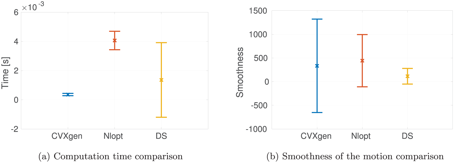
IK solver performance. In the first set of simulations, the performance of the three solvers of (17) (CVXgen, Nlopt, and the DS (20)) are assessed in terms of computation time and the smoothness of the generated joint motions. The initial velocity of the object is fixed but the initial position is randomly chosen within the range of $[-3.5\pm 0.05-0.45\pm 0.050.8\pm 0.05]$ m. The simulation is repeated five times for each solver which results in more than $5*35,000$ data points. The termination tolerance of the solvers is set to ${10}^{-4}$ . The computation time of each solver is illustrated in Figure 17a. As it was expected, CVXgen is the fastest solver and it takes about $0.000358\mathrm{s}$ for it to solve (17) in average. The performance of the our implementation of (20) takes approximately $0.00092\mathrm{s}$ to solve (17). As initialization of the DS (20) plays an important role in the convergence duration, the standard deviation of the computation time of (20) is much higher than the other two approaches. The smoothness of the trajectory $L$ is assessed by $\mathcal{S}=\frac{\mathrm{std}(\stackrel{.}{L})}{\mathrm{mean}(\stackrel{.}{L})}$ , where a smaller value of it indicates a smoother motion. As it is shown in Figure 17b, the result of (20) is much smoother than the other methods. It was expected as (20) calculates the desired motion at the acceleration level. Hence, the output of (20) can directly be transmitted to the robots, but the outputs of either Nlopt or CVXgen need to be filtered. As the computation power was the main criterion for choosing the IK solver for us, we mostly used CVXGEN during the experiments.

Fig. 17.

The results of performance of the solvers for (17) in terms of computation time and the smoothness of the motion. DS stands for the DS (20).

Fig. 18.

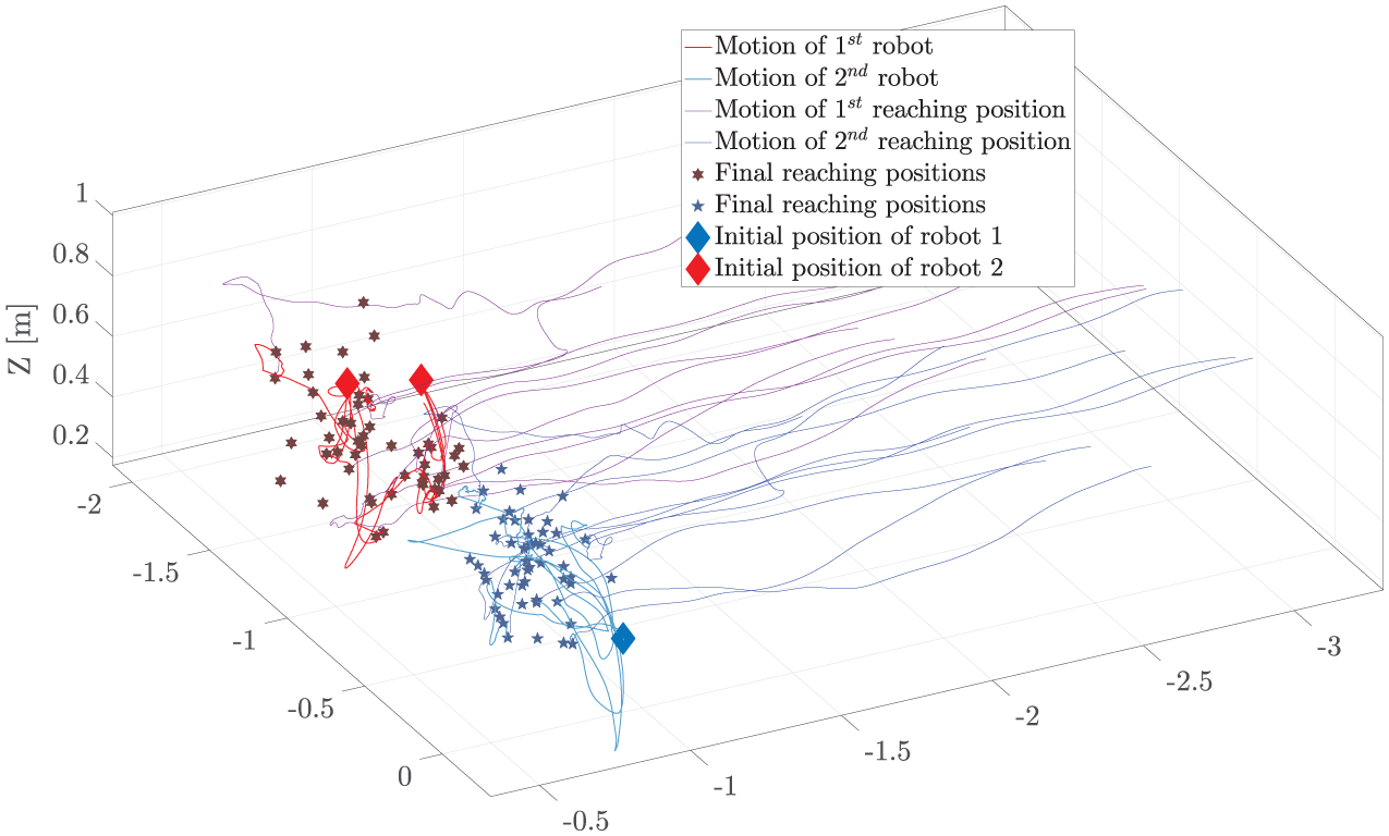
Spatial Variation of final intercept points. For clarity, only ten runs (i.e. trajectories) of the object and robots’ motions are shown. For each run a different object trajectory and final intercept points were observed. Experimental results verified that the robots intercept the object in synchrony.

Fig. 19.

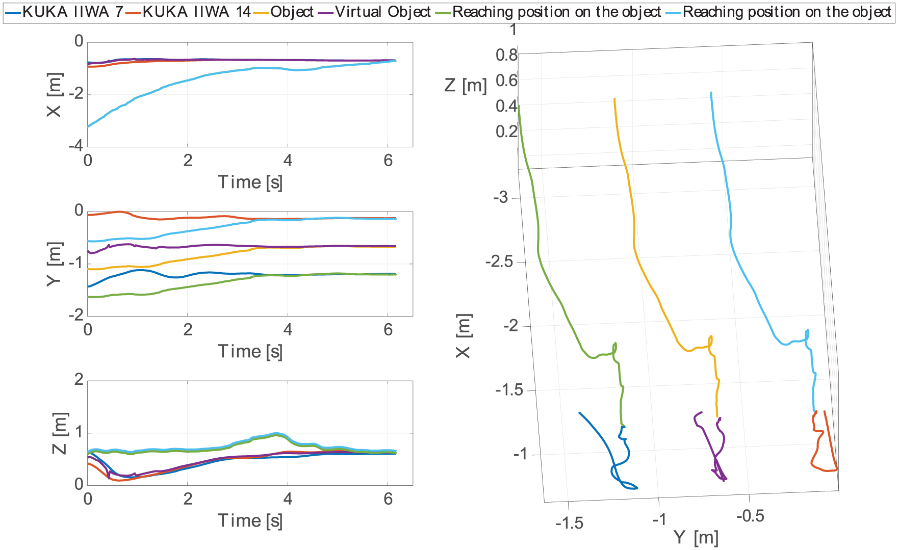
The position of the end-effector, the virtual object generated by (2) and (11), respectively. These trajectories are illustrated from the first point until the stop point. As expected, both arms intercept the reaching positions on the object at the same time. In order to avoid any internal forces, the robots are stopped once the fingers are closed on the object.

Fig. 20.

Snapshots from the systematic assessment experiment. The objects are a bumper, a front panel, and a fender in (a), (b), and (c), respectively. The robots are stopped when the hand and the gripper are closed. A corresponding video is available as Extension 2.

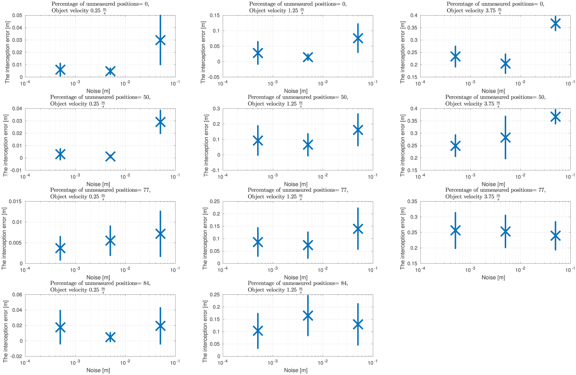
Sensitivity to noise. In the second set of simulations, the robustness of the framework to noise and unmeasured object position is assessed. The simulation is repeated $165$ times in total for three different object velocities, i.e. $0.25$ , $1.25$ , and $3.75{\mathrm{m\; s}}^{-1}$ . Results from this evaluation indicate that the interception error is directly correlated to the percentage of unmeasured object points and the velocity of the moving object (see Figure 21). Thus, the faster the object, the more sensitive the system is to tracking inaccuracies.

Fig. 21.

The interception error is the average of the minimum distance between the box and the end-effectors. The initial positions of the box are randomly chosen within the range of ${[-3.5\pm 0.1-0.45.0\pm 0.10.8\pm 0.1]}^{\mathrm{T}}$ m. The distance between the arms and the size of the box are same as the bumper scenario. The simulations are repeated for each combination of three object’s speeds, three noise powers, and four percentages of unmeasured positions. We only consider trials when the box passes through the robots workspaces. The measurement noise is simulated with pseudo-random values within the range of $\pm 0.05$ , $\pm 0.005$ , and $\pm 0.0005$ m. The results of the worse case are not illustrated as the robots were not able to follow the object, i.e. the worse case is when the percentage of unmeasured position is $85\%$ and the box’s velocity is $3.75$ m s⁻¹.

7. Summary and discussion

In this paper, we proposed a DS-based unified framework for generating motion of multiple robotic arms to either coordinately reach a moving object or reach stably to a desired point. If provided with robotic arms that can travel fast enough, our algorithm can select the most feasible robotic arms to intercept the object in coordination and with the desired velocity aligned to the object while any collision between the arms are avoided. For selecting the most feasible robotic arms, we define a parameter (i.e. the synchronization parameter) to assign the robots to the appropriate behavior, i.e. the asynchronous or synchronous behaviors. The synchronization parameter varies between zero and one based on the feasibility criteria.

The stability and convergence of the proposed DS depends on ensuring conditions (13) hold. As there are no constraints on the magnitude of the eigenvalues $(|{\lambda }_{A_{ij}}|)$ of $A_{ij}\forall (i,j)\in \{(1,1),(1,2),\dots ,(N_R,d_{s_{N_R}})\}$ , there is no analytical proof that (11) is fast enough to converge to $\gamma {\xi }^O$ in time. To address this challenge, a potential direction would be to estimate the parameters of (11) with respect to the stability and the convergence rate constraints. One way to calculate the convergence rate of a DS is to prove that it is exponentially stable (Khalil, 2002).

To solve the QP problem, we used three different approaches. First a DS-based approach (20). Second, a non-linear programming solver (Johnson, 2016). The third approach was CVXGEN, introduced in Mattingley and Boyd (2012). Each of these approaches has its own advantages and disadvantages. Using the first approach is advantageous in the way that the passivity of the DS can be proven. Hence, the unified framework remains passive and stable as long as the robots are passive. In addition, the first approach result in smoother joint motions. The main advantage of the second approach is its interface. Nlopt is very user friendly and it is possible to test several solvers, but it is computationally costly. The main advantage of the third approach is the computational cost. As it has been shown in Mattingley and Boyd (2012), CVXGEN is computationally very efficient. The main shortcoming of the third approach is the stability of the closed-loop system, which cannot be proven; however, we have not seen any unstable behaviors during the real-world evaluations or the simulations.

Throughout the proofs, we assume that the intercept point is a fixed attractor. However, due to the imperfect prediction of the object trajectory, the feasible intercept postures need to be iteratively updated. Nevertheless, this does not affect the convergence of the system for two main reasons. First, when $\gamma <1$ the new feasible intercept point is chosen in the vicinity of the previous ones, i.e. the convergence rate is much faster than the rate of update. Second, when the object is reachable, $\gamma =1$ , the virtual object converges to the real object and the position of the intercept point does not affect the convergence. If we assume that the object trajectory is predictable, one can simply generalize a single-robot arm feasible posture extraction (Kim et al., 2014) for multiple arms to extract the intercept posture. However, the proposed algorithm is not restricted to this assumption. In this work, the feasible intercept point is calculated to make sure that, first, the object is passing through the robots’ reachable space and, second, to move the robots in advance to the vicinity of this point to avoid highly accelerated motions.

In this paper, we control the motion of the arm from initial condition (palm open, robots far from the object) to the point when the arms reach the object and the fingers are about to close on the object. Hence, there are no interaction forces (which would arise once in contact with the object). Once the fingers close on the object, the robots–object system become a closed kinematic chain. In this case, devising an appropriate force controller is necessary to coordinate the robots. Future work in multi-arm manipulation will be directed to address the challenges of devising an appropriate force controller and the transition between the position and force controller.

One of the main advantages of the proposed framework is the computational cost. The implementation shows that the overall computation is rapid, thus enabling us to not only compute the feasible intercept point, the reaching motion and solve centralized IK problem, but also to control a ( $7+7+16+1=$ ) 33-DOF system with one 3.4 GHz i7 PC.

Finally, we are currently working on improving the performance of (15), by learning its parameters via a convex optimization problem with respect to the workspace constraint of the robots. With this approach, we could ensure that the performance of the DS is optimal and the generated motion is not infeasible for the robots to follow.