Generalized graph SLAM: Solving local and global ambiguities through multimodal and hyperedge constraints

Abstract

Research in Graph-based Simultaneous Localization and Mapping has experienced a recent trend towards robust methods. These methods take the combinatorial aspect of data association into account by allowing decisions of the graph topology to be made during optimization. The Generalized Graph Simultaneous Localization and Mapping framework presented in this work can represent ambiguous data on both local and global scales, i.e. it can handle multiple mutually exclusive choices in registration results and potentially erroneous loop closures. This is achieved by augmenting previous work on multimodal distributions with an extended graph structure using hyperedges to encode ambiguous loop closures. The novel representation combines both hyperedges and multimodal Mixture of Gaussian constraints to represent all sources of ambiguity in Simultaneous Localization and Mapping. Furthermore, a discrete optimization stage is introduced between the Simultaneous Localization and Mapping frontend and backend to handle these ambiguities in a unified way utilizing the novel representation of Generalized Graph Simultaneous Localization and Mapping, providing a general approach to handle all forms of outliers. The novel Generalized Prefilter method optimizes among all local and global choices and generates a traditional unimodal unambiguous pose graph for subsequent continuous optimization in the backend. Systematic experiments on synthetic datasets show that the novel representation of the Generalized Graph Simultaneous Localization and Mapping framework with the Generalized Prefilter method, is significantly more robust and faster than other robust state-of-the-art methods. In addition, two experiments with real data are presented to corroborate the results observed with synthetic data. Different general strategies to construct problems from real data, utilizing the full representational power of the Generalized Graph Simultaneous Localization and Mapping framework are also illustrated in these experiments.

1. Introduction

When robots face more complex, unstructured and dynamic environments while expanding their workspace, the problem of Simultaneous Localization and Mapping (SLAM) becomes even more relevant and significantly more difficult at the same time. There is a clear need for efficient and, most of all, robust SLAM methods that are able to generate a useful map, even under erroneous data association decisions on any level in the SLAM process.

Graph-based SLAM (Frese, 2006; Grisetti et al., 2010, 2007b; Kaess et al., 2008; Kümmerle et al., 2011; Lu and Milios, 1997; Olson et al., 2006) has been the method of choice in the latest literature on SLAM in dynamic environments (Walcott-Bryant et al., 2012), portable SLAM systems for humans (Fallon et al., 2012), SLAM with micro aerial vehicles (MAV) (Fraundorfer et al., 2012; Leishman et al., 2012), as well as underwater SLAM (Hover et al., 2012; Pfingsthorn et al., 2012). All of these applications can benefit significantly from an improved robustness of graph optimization methods for SLAM. For these reasons, robust graph optimization or inference for graph-based SLAM has very recently become a strong research focus (Latif et al., 2012a,b; Olson and Agarwal, 2012, 2013; Pfingsthorn and Birk, 2013; Sunderhauf and Protzel, 2012a,b). While a detailed discussion is given in Section 2, these methods fall into roughly two categories.

In one category with methods by Sunderhauf and Protzel (2012a,b), Latif et al. (2012a,b) and partially by Olson and Agarwal (2012, 2013), inconsistent graph constraints are simply discounted during optimization. This category is roughly comparable to iteratively reweighted least squares (Huber and Ronchetti, 2009) or least trimmed squares (Rousseeuw and Leroy, 2005), both traditional robust regression techniques that are used for a wide range of optimization problems.

The other category by Pfingsthorn and Birk (2013) and partially by Olson and Agarwal (2012, 2013) allows multiple components per constraint, either as a multimodal Mixture of Gaussians (MoGs) (Pfingsthorn and Birk, 2013), or a so-called multimodal Max-Mixture (Olson and Agarwal, 2012, 2013). The Max-Mixture method however greedily reevaluates, in each step of the iteration, which of the mixture components should be used. It therefore approaches robust SLAM in a similar way to the first category, in the sense that the components are discounted during optimization and the robust optimization is incorporated in the SLAM backend. The multimodal MoGs of Pfingsthorn and Birk (2013) are in contrast handled in a novel discrete optimization stage that is introduced as a new midstage between the SLAM frontend and backend.

This article presents a general framework for SLAM under ambiguous data associations. It is named “Generalized Graph SLAM” for two reasons. First and foremost, it offers a generic solution to deal with arbitrary forms of outliers in Graph SLAM that otherwise would have to be handled by very application specific heuristics in the frontend. As we will see in the experiments sections, it is quite difficult in many application domains to avoid local as well as global outliers, i.e. outliers in sequential motion estimates through sensor data registration or odometry as well as in non-sequential motion estimates in loop closures. Additionally, the rejection of outliers in the frontend usually requires a significant amount of effort and parameter tuning, which can be substantially eased by the use of Generalized Graph SLAM. Secondly, the representation used in the framework generalizes other state-of-the-art robust formalizations of Graph SLAM. It therefore provides a basis for a general formal treatment of the problem representation.

Generalized Graph SLAM contains the first formal introduction of how uncertain loop closures can be modeled using hyperedges. The representation and its semantics build upon the authors’ previous work on multimodal MoG constraints (Pfingsthorn and Birk, 2013) and generalizes it - as well as the formalizations used in other state-of-the-art methods in robust SLAM as discussed in detail in Section 3.5. The novel hyperedge representation allows us to encode global ambiguities, i.e. to represent multiple alternative hypotheses about possible loop closures including the Null hypothesis of no feasible closure. The multimodal MoG constraints in contrast deal with local ambiguities, i.e. they handle different alternative hypotheses about the motion a robot may have undergone between two observations. Using these two complementary approaches, the new Generalized Graph SLAM framework is designed to represent local as well as global ambiguities in a single coherent manner.

A crucial aspect is not only the representation of ambiguities but also the question of how to optimize under their presence. To solve this, the Prefilter method that was introduced for local ambiguities represented as MoGs in the authors’ previous work (Pfingsthorn and Birk, 2013) is extended here to select globally consistent constraints from the novel multimodal hypergraphs in a comprehensive unified way. This Generalized Prefilter is introduced as a new midstage between the SLAM frontend and backend to perform a discrete optimization. It performs a minimum spanning tree traversal of the multimodal hypergraph using the total number of mixture components per edge as a weight, during which a combinatorial tree is generated with each leaf representing the exact component (including the Null hypothesis choice for hyperedges) chosen in the hypergraph traversal. Each component carries relative pose information used to assign poses to vertices visited in the traversal. This combinatorial tree is searched using beam search, where only the best N leafs, i.e. the ones with the highest joint probability given the computed poses, are kept at each iteration of the hypergraph traversal. When the traversal completes, the best remaining leaf of the combinatorial search tree, and thus the component choices along the corresponding hypergraph traversal, is picked. The computed poses on the path to this leaf are assigned to the vertices in the graph, and the remaining ambiguous edges are disambiguated by picking the component that best explains the estimated poses of the related vertices. Finally, the disambiguated unimodal graph including the computed vertex poses is then returned for subsequent continuous optimization in a standard SLAM backend.

In this article, the Generalized Prefilter is systematically compared with the current state-of-the-art robust graph SLAM methods using synthetic and real data. The experiments with synthetic data show that the Generalized Prefilter method is both significantly more robust and faster than other robust state-of-the-art methods, especially as the graph complexity increases. Experiments on the standard synthetic Sphere2500 dataset (Kaess et al., 2012) that mirror those used to evaluate other robust methods show that the Generalized Prefilter method performs as well as the employed backend alone, in the case that all non-sequential edges are hyperedges with a single simple constraint and a Null hypothesis component. As soon as a single MoG component is introduced, the Generalized Prefilter method performs significantly better than other tested methods. Furthermore, approaches to generate multimodal hypergraphs in the Generalized Graph SLAM framework from two real world datasets are presented and discussed. The first experiment involves range-based 3D SLAM in an urban scenario using the Bremen City dataset (see Section 7). The second experiment applies visual 2D SLAM to an underwater dataset from the Ligurian Sea (see Section 8). These two experiments with real world data also include comparisons with competing methods and show the increased robustness and speed of the Generalized Prefilter method.

In addition, they illustrate cases of how Generalized Graph SLAM can be employed in practice in various applications. Specifically, four general strategies are presented. The first two strategies show how multimodal MoG constraints can be generated, the second two strategies show how hyperedges can be generated.

1. Ranked registration results: Some registration techniques can generate a list of ranked results, e.g. HSM3D (Censi and Carpin, 2009), SRMR (Bülow and Birk, 2013), Spherical Harmonics (Kostelec and Rockmore, 2003, 2008), or plane-matching (Pathak et al., 2010). When the ranked list delivers no clear best result, the different alternatives can be incorporated as choices which form a multimodal constraint. This is illustrated with plane-matching in the experiment using the Bremen City dataset.

2. Complementary motion estimates: Using two (or more) registration methods in parallel, respectively combining, e.g. one registration method and odometry, leads to complementary motion estimates. This is a strategy that is widely used in SLAM applications. However, the standard approach of probabilistic fusion of the estimates can severely degrade performance if one of them is occasionally wrong. Incorporating the estimates as alternative choices when they are not congruent leads to superior performance, as shown in our experiments. RANSAC (Fischler and Bolles, 1981) with an affine transformation model on SURF (Bay et al., 2006) features and iFMI (Bülow et al., 2009) as two complementary registration methods in the visual SLAM experiment on the Ligurian Sea data are used to demonstrate this general use case to generate multimodal edges.

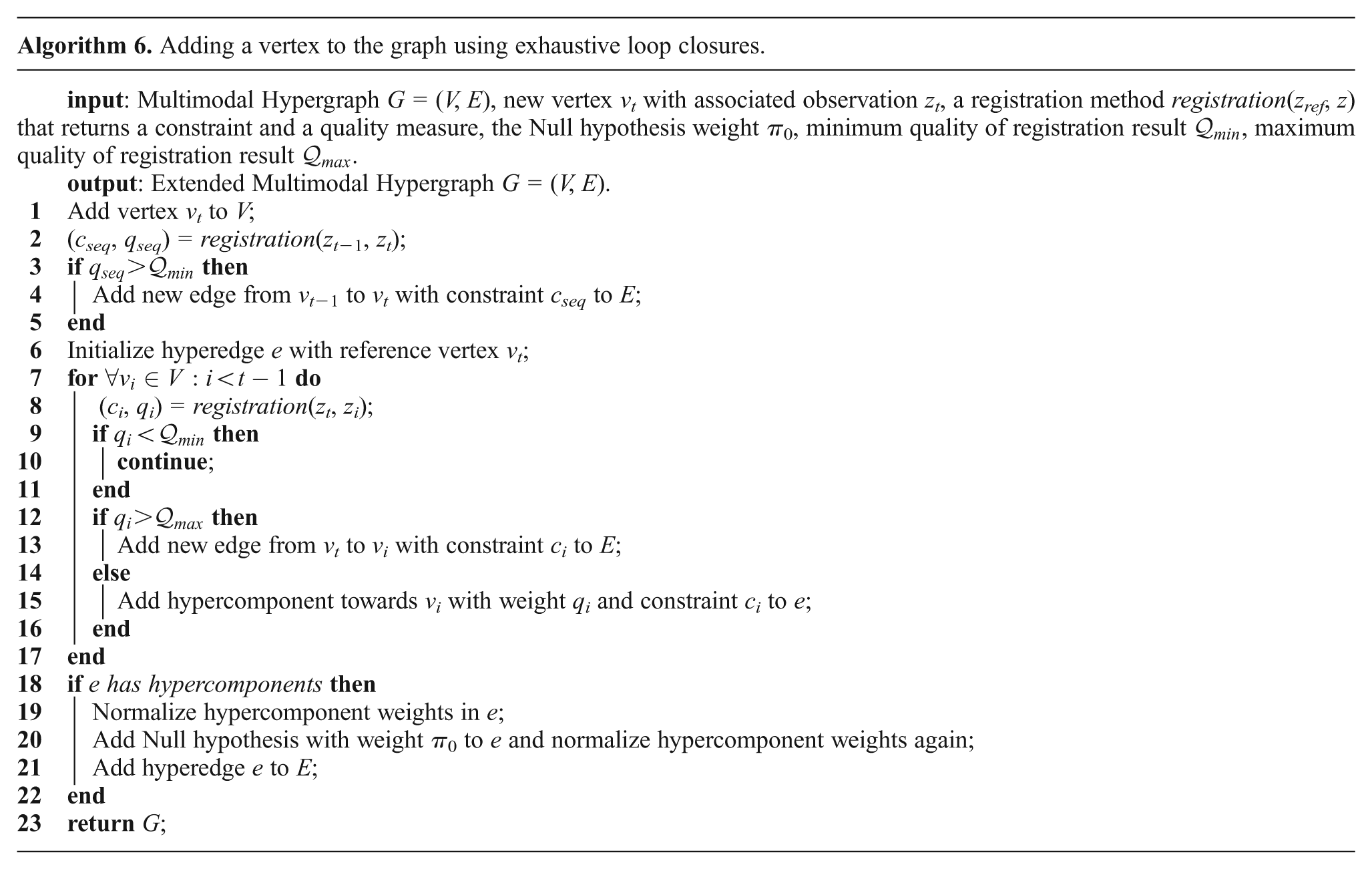
3. Exhaustive loop closing: When the graph is relatively small, it is feasible to exhaustively register all data with each other, i.e. to exhaustively try out all possible loop closures. This can be seen as an extreme case of the next point, Lenient Place Recognition, but it is treated separately here to highlight this naive baseline of not using any place recognition method. Additionally, such an exhaustive strategy leads to a very high likelihood that all possible loop closures are included in the graph. This use case is included in the experiment using the Bremen City dataset with plane-matching.

4. Lenient Place Recognition: In general, place recognition methods usually allow us to trade-off recall and precision. Lenient parameter settings of the place recognition method allow us to find significantly more true positives at the cost of also generating false positives. This use case is illustrated with the example of the popular FabMAP method (Cummins and Newman, 2011) that is used in the Ligurian Sea experiment for place recognition.

The rest of this article is structured as follows. Section 2 describes related work in robust Graph-based SLAM. Section 3 introduces the representation of local and global ambiguities through multimodal hyperedges in the Generalized Graph SLAM framework. The Generalized Prefilter method for the discrete optimization of multimodal hypergraphs in a SLAM midstage is described in Section 4. This is followed by a systematic investigation of the performance of this method relative to the state-of-the-art methods using synthetic data with both global and local ambiguity in Section 5. Section 6 describes general methods to generate multimodal or hyperedge constraints from real data. Sections 7 and 8 present results from real world experiments with these methods. Finally, the article is concluded in Section 9.

Preliminary reports on some of the work and results with real world data have been published in two conference papers (Pfingsthorn and Birk, 2014; Pfingsthorn et al., 2014). This article contains a significantly more detailed and unified description of the work, as well as rigorous systematic experiments in addition to the content of the previously published conference papers.

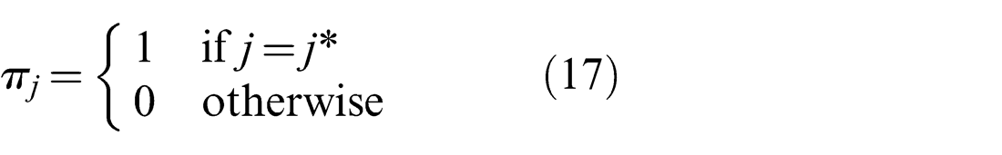
2. Related work

The robust SLAM methods by Pfingsthorn and Birk (2013), Olson and Agarwal (2012, 2013), Latif et al. (2012a,b) and Sunderhauf and Protzel (2012a,b) improve upon traditional Graph SLAM methods by providing ways to filter out or discount inconsistent graph constraints during optimization.

While not specified exactly in the paper, the g²o graph optimization library by Kümmerle et al. (2011) chooses a traditional robust optimization approach by applying an iteratively reweighted least squares (IRLS) method (Huber and Ronchetti, 2009). Their approach allows weighting the individual terms of the cost function by the computed residuals and reducing the influence of large residuals. More than one of these robust kernels are implemented, e.g. the Huber or the Cauchy kernel (Huber and Ronchetti, 2009). Thus, inconsistent constraints are weighted less, which allows the method to converge to a reasonable result when some outliers are present.

Sunderhauf and Protzel (2012a,b) choose a more explicit reweighting scheme where the weight of a cost function term is controlled as part of the state vector during optimization. Instead of using the value of the local residual to scale the impact of it in the total cost function, switching variables are introduced that are explicitly part of the state. A linear function is used to map the continuous domain of the switch variable to a weight between 0 and 1. With this approach, depending on the switch variable’s sign, the individual constraints are rather suddenly and explicitly “switched on” or “switched off”, which stands in contrast to the more subtle and implicit reweighting in g²o. A recent extension of this idea by Agarwal et al. (2013) incorporates the switch variable into a robust kernel (M-estimator) similar to the Huber or Cauchy kernels mentioned above.

In the authors’ previous work (Pfingsthorn and Birk, 2013), a novel multimodal extension of the traditionally unimodal constraints used in Graph-based SLAM was introduced. This was combined with a novel discrete optimization stage between the SLAM frontend and backend in the form of the Prefilter algorithm. Standard methods assume that a constraint in the graph is inherently correct and just uncertain due to noise; it can therefore be represented by a single underlying normal distribution. Instead, a multimodal MoG is used that allows multiple mutually exclusive options (modes) in each edge. This work also introduced the concept of local ambiguity versus global ambiguity, where the presented approach using MoGs is used to solve the local ambiguity problem, i.e. the handling of different motion alternatives between two subsequent robots, respectively sensor poses.

Several methods are outlined to solve SLAM with locally ambiguous registration results that are expressed in multimodal MoGs including the Prefilter method, which is shown to be very robust. A core aspect of the Prefilter method is that it operates as a separate discrete optimization stage between the SLAM frontend and backend, i.e. it is used to discard inconsistent components in the MoG constraints before optimization, which is related to least trimmed squares (Rousseeuw and Leroy, 2005). Olson and Agarwal (2012, 2013) take a similar approach by allowing multiple single normal distributions in one constraint in the graph. However, in their method the decision as to which of the constraint distributions should be used is greedily re-evaluated in each step of the iteration, i.e. the method is like other approaches to robust SLAM incorporated in the SLAM backend. Instead of using a weighted sum of normal distributions as is the case with MoGs, their approach only uses the component which contributes the maximum probability to the current estimate, thus the name Max-Mixture. Max-Mixtures have the disadvantage that they are chosen greedily given the current estimate, requiring good initial conditions to allow convergence. Olson and Agarwal (2012, 2013) also describe the idea that multiple loop closing constraints may be combined into one using a multimodal Max-Mixture, effectively representing a hyperedge but not explicitly using the name nor describing the idea in any formal way.

Latif et al. (2012a, 2013, 2012b) present a method called RRR to generate clusters of temporally close loop-closing constraints and check these for spatial consistency. The method makes the rather significant assumption that sequential constraints are generated using odometry and are always without outliers. A traditional ${\mathcal{X}}^2$ error metric is used to identify outliers in each cluster of loop-closing constraints. By explicitly making a binary decision about the inclusion or rejection of individual constraints, the method is highly related to the least trimmed squares method.

3. Representation of local and global ambiguities

3.1. Background: Traditional Graph-based SLAM

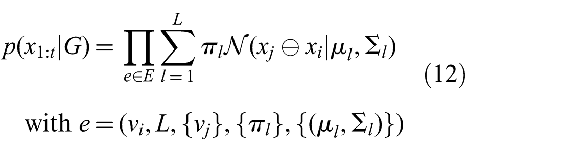
Graph-based SLAM methods (Frese, 2006; Grisetti et al., 2010, 2007b; Kaess et al., 2008; Kümmerle et al., 2011; Lu and Milios, 1997; Olson et al., 2006) use a graph data structure called a pose graph. Formally, a pose graph is an undirected graph G = (V, E) consisting of vertices V and edges E. The vertices v_i ∈ V denote poses where the robot has obtained sensor observations z_i. A pose estimate x_i is also associated with the vertex and thus is a tuple v_i = (x_i, z_i). In addition to the vertices it connects, each edge e_k ∈ E contains a constraint c_k on the pose estimates of the associated vertices, usually derived from the corresponding sensor observations. Thus e_k = (v_i, v_j, c_k). While the graph itself is undirected, the edge has to declare a sort of observation direction, the direction in which the constraint was generated, often called the reference frame of the constraint. In case the edge is traversed in the reverse observation direction, the constraint c must be inverted. The representation of the constraint determines what this inverted constraint entails.

The joint probability of any pose graph G is

$$p(x_{1:t}|G)=\underset{(v_i,v_j,c_k)\in E}{\Pi }p(x_j\ominus x_i|c_k)$$

(1)

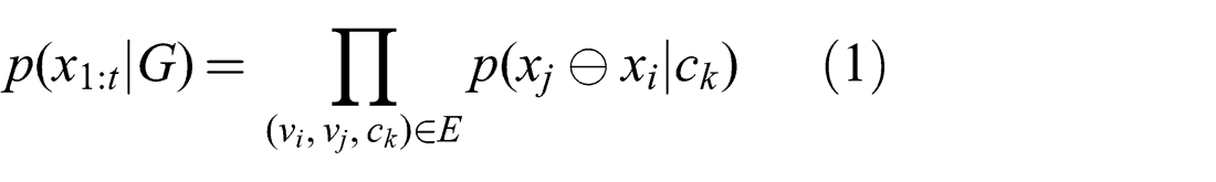
where p(x_j⊖x_i|c_k) is the specific probability distribution of the constraint c_k on edge e_k ∈ E, and ⊖ is the pose difference operator.

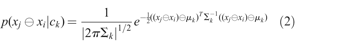
In the traditional case, the constraints are represented by a multivariate normal distribution with mean ${\mu }_k$ and covariance ${\Sigma }_k$ , so

$$p(x_j\ominus x_i|c_k)=\frac{1}{|2\pi {\Sigma }_k{|}^{1/2}}{e}^{-\frac{1}{2}{((x_j\ominus x_i)\ominus {\mu }_k)}^T{\Sigma }_k^{-1}((x_j\ominus x_i)\ominus {\mu }_k)}$$

(2)

This results in a very convenient negative log likelihood formulation that can be directly used in a general non-linear least squares solver

$$-\ln p(x_{1:t}|G)\approx \sum _{(v_i,v_j,c_k)\in E}{((x_j\ominus x_i)\ominus {\mu }_k)}^T{\Sigma }_k^{-1}((x_j\ominus x_i)\ominus {\mu }_k)$$

(3)

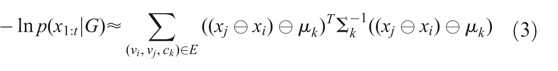
which is in effect the sum of squared mahalanobis distances.

Traditionally, Graph-based SLAM methods have almost exclusively used this representation (Frese, 2006; Grisetti et al., 2010, 2007b; Kaess et al., 2008; Kümmerle et al., 2011; Lu and Milios, 1997; Olson et al., 2006). Since minimizing equation (3) represents a weighted least-squares optimization problem, a number of classical methods are applicable as well, including the Gauss-Newton, Levenberg-Marquardt and Conjugate Gradient methods (Björck, 1996; Nocedal and Wright, 1999).

Fig. 1.

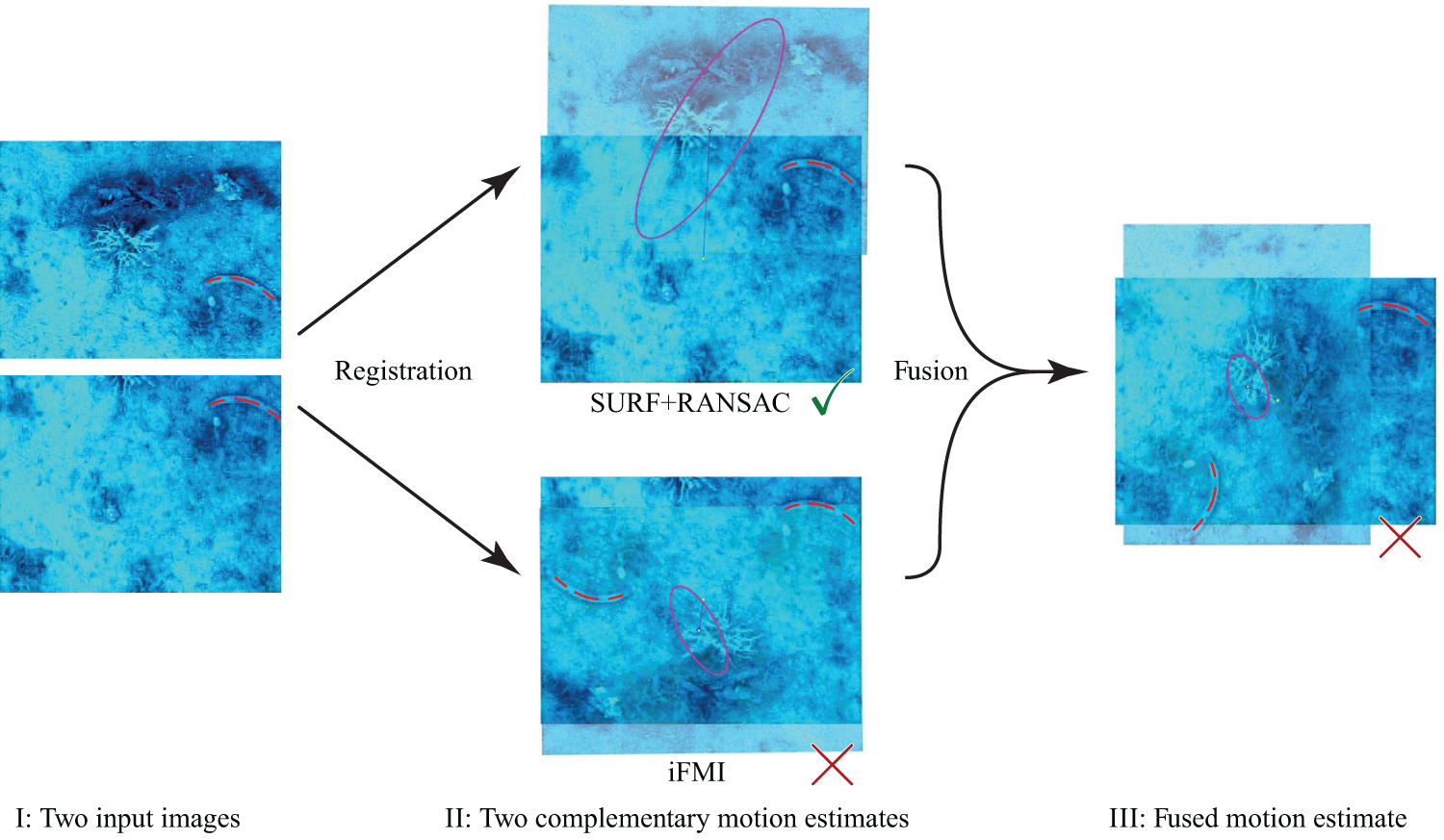
An example of local ambiguity, based on two complementary registration techniques for motion estimation. The same situation can arise with a single registration method that is combined with an odometry estimate. I: Two frames from the Ligurian Sea dataset (see also Section 8). II: Registration results from two methods: A correct registration result using SURF and RANSAC with an affine model (top) and a failed registration using iFMI (bottom). III: Fusion result, which is inferior to keeping both estimates as mutually exclusive alternatives. The effect is amplified in this example as SURF+RANSAC had a high uncertainty and iFMI a low uncertainty (purple ellipses), and thus the fused estimate is closer to the wrong result of iFMI. Note the highlighted feature (red dashed arc) in the images for visual verification of the motion estimates.

3.2. Local ambiguity and global ambiguity in SLAM

A major source of errors in Graph-based SLAM is faulty data association. In the traditional case described above, a single faulty constraint, e.g. from an iterative registration method that converged to a local optimum or an unreliable place recognition method, can destroy the complete map.

Specifically, two types of data association errors are identified here: a) Errors in identifying common data in two consecutive sensor observations (local ambiguity) and b) errors identifying common data in temporally distant sensor observations (global ambiguity). This section describes each of these error sources and motivates the foundations for the Generalized Graph SLAM framework.

Local ambiguity corresponds to the case where two consecutive sensor observations lead to multiple possible motion estimates, e.g. due to different registration results. A motion estimate of two such observations is called locally ambiguous if these ambiguities can not be resolved using only information present in the observations themselves. Specifically, the two observations may contain some symmetry or share only a few weak features, such that a single data association hypothesis that is significantly more likely than others does not exist. In other words, the registration cost function has multiple significant optima when applied to this pair of observations. This is true whether the cost function is combinatorial as in the feature-based case, discrete as in the case with correlational or spectral methods, or continuous as in the case of ICP (Besl and McKay, 1992) or NDT (Magnusson et al., 2007). Such multiple optima may be represented as a multimodal MoG probability distribution for the corresponding constraint (Pfingsthorn and Birk, 2013)

$$p(x_i|x_{i-1})=\sum _{m=1}^{M_k}{\pi }_m\mathcal{N}(x_i\ominus x_{i-1}|{\mu }_m,{\Sigma }_m)$$

(4)

with $\sum {\pi }_m=1$ . In the case of continuous cost functions, each mean μ_m corresponds to an optimum in the registration cost function, Σ _m corresponds to the inverse of the Hessian at that point and the weight π_m should be proportional to the value of the registration cost function at μ_m. However, other methods to arrive at such MoG models for multimodal registration results are possible.

Global ambiguity corresponds to the case of uncertain loop closures, where the current sensor observation may or may not show the same section of the environment as one or many temporally distant sensor observations (see figure 2 for an example). Repetitions in the environment or a low number of previously seen features in the observations could result in multiple likely loop hypotheses that may be mutually exclusive, e.g. corridor intersections at different floors.

Fig. 2.

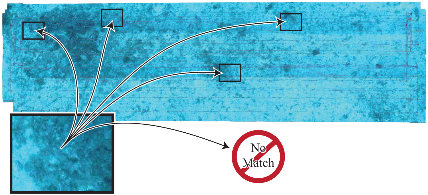
A visualization of global ambiguity, corresponding to a general loop detection problem. The image (left) either corresponds to a previously visited location (arrows going towards the map), or represents a newly visited location (arrow leading to “No Match”). In the Generalized Graph SLAM framework, all correspondences relating to previous locations are collected as hypercomponents with corresponding weights, and the option “No Match” is expressed as the Null hypothesis in the hyperedge.

Formally, there exists a probability mass function (PMF) which is defined over the events that the current sensor observation matches individual previous ones and the event that the current observation is completely new. This PMF can be represented as the weights π_m of a more generalized mixture over all previous poses (where observations were made) and an uninformative uniform distribution representing the Null hypothesis

$$p(x_i|x_{1:i-1})={\pi }_0\mathcal{U}({\mathbb{R}}^d)+\sum _{j=1}^{i-1}{\pi }_{j}p(x_j\ominus x_i|c_j)$$

(5)

with ${\sum }_0^{i-1}{\pi }_j=1$ , and where x_1:i−1 are all poses from vertex v₁ to v_i−1, p(x_j⊖x_i|c) is any probability distribution representing a registration result, π₀ is the weight of the Null hypothesis and $\mathcal{U}({\mathbb{R}}^d)$ is the uniform distribution over all real numbers of the same degree of freedom, d, as the poses.

Other distributions can be employed to represent the Null hypothesis, e.g. a normal distribution with a very large variance matrix as proposed in the informal description by Olson and Agarwal (2012, 2013), which may be somewhat easier to use in practice than a uniform distribution.

Note that local ambiguity may also occur in the registration result referenced in the global ambiguity case, i.e. a loop closure may not only lead to several candidate places but each of the hyperedge components may in addition have multimodal results for each underlying registration. Local and global ambiguities therefore are orthogonal problems, both or either may or may not occur in any given SLAM application.

3.3. Modeling uncertain loop constraints as hyperedges

Exhaustively modeling the complete mixture from equation (5) for all previous poses is wasteful. Most of the weights π_j will be zero or very close to zero. Instead, a more compact representation is needed.

Graph theory presents a fitting concept in this case, namely a hyperedge. Formally, a hyperedge is a set of vertices that are connected. Thus, instead of every edge e ∈ E consisting of exactly two endpoints v_i, v_j and the associated constraint c_k as described in section 3.1, a hyperedge in a pose graph is defined as a tuple

$$e_k=(v_i,N,\{v_j\},\{{\pi }_j\},\{c_j\})$$

(6)

{v_j} is the set of vertices the reference vertex v_i is connected to by this edge, and N = |{v_j}|. The weight of the Null hypothesis is implicitly given by ${\pi }_0=1-\sum {\pi }_j$ , with $\sum {\pi }_j\le 1$ . Note that in the case where N = 1, i.e. there is no ambiguity with which older vertex v_j the reference vertex v_i should be connected to, is explicitly covered as well, while still allowing for discounting of this one constraint by reducing the weight π₁. Also note that due to the geometric interpretation of the edge, an observation direction is still necessary, so v_i is defined as the reference of the hyperedge and the base frame of the relative poses represented in the constraints.

For a single hyperedge, equation (5) becomes

$$p(x_i,\{x_j\}|e)=(1-\sum _{j=1}^N{\pi }_j)\mathcal{U}({\mathbb{R}}^d)+\sum _{j=1}^N{\pi }_{j}p(x_j\ominus x_i|c_j)$$

(7)

Note that the hyperedge relates all connected vertices, not exhaustively all previous vertices as in equation (5), thus the probability density is defined over the poses of the reference vertex v_i and the related vertices {v_j}. When applied to the graph as a whole, this becomes

$$\begin{array}{cc}\multicolumn{1}{c}{p(x_{1:t}|G)}& =\underset{e\in E}{\Pi }p(x_i,\{x_j\}|e)\hfill \\ \multicolumn{1}{c}{}& =\underset{e\in E}{\Pi }[(1-\sum _{j=1}^N{\pi }_j)\mathcal{U}({\mathbb{R}}^d)+\sum _{j=1}^N{\pi }_{j}p(x_j\ominus x_i|c_j)]\hfill \end{array}$$

(8)

$$\approx \underset{e\in E}{\Pi }\sum _{j=1}^N{\pi }_{j}p(x_j\ominus x_i|c_j)$$

(9)

Since $\mathcal{U}({\mathbb{R}}^d)$ is practically zero everywhere (technically $\frac{1}{\infty }$ ) and therefore has no impact computationally, especially since its gradient is zero, the term corresponding to the Null hypothesis is dropped. This means that the expression looks exactly like a regular mixture, with the difference that $\sum _{j=1}^N{\pi }_j\le 1$ instead of $\sum _{j=1}^N{\pi }_j=1$ . In practice, this approximation does not change the gradients of the expression, and has negligible impact on the computed value.

Alternatively, the mixture mean and a possibly scaled mixture covariance (Carreira-Perpinan, 2000) can give rise to a single large normal distribution to represent the mixture and serve as a good quasi-uniform Null hypothesis. However, this alternative has not been investigated so far.

In the following, each p(x_j⊖x_i|c_j) is called a hypercomponent to distinguish between components in a hyperedge and in a MoG constraint mixture. π_j will be referred to as the hypercomponent weight.

3.4. Representation in the Generalized Graph SLAM framework

Without loss of generality, it is assumed in the Generalized Graph SLAM framework that all edges in a generalized pose graph are hyperedges and all the constraints c_j of each edge are multimodal MoG constraints. All less complex cases can be modeled as such a hyperconstraint containing MoGs. Here, the cases with N = 1 (i.e. no global ambiguity) and M_k = 1 (i.e. no local ambiguity) are explicitly included.

For this generalized graph, the joint probability then becomes

$$\begin{array}{cc}\multicolumn{1}{c}{p(x_{1:t}|G)}& =\underset{e\in E}{\Pi }\sum _{j=1}^N{\pi }_j\sum _{m=1}^{M_k}{\pi }_m\mathcal{N}(x_j\ominus x_i|{\mu }_m,{\Sigma }_m)\hfill \\ \multicolumn{1}{c}{\mathrm{with}e}& =(v_i,N,\{v_j\},\{{\pi }_j\},\{c_j\})\hfill \end{array}$$

(10)

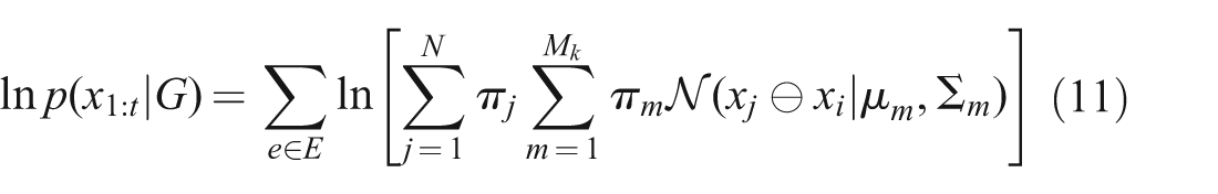
Similarly for the joint log probability

$$\ln p(x_{1:t}|G)=\sum _{e\in E}\ln [\sum _{j=1}^N{\pi }_j\sum _{m=1}^{M_k}{\pi }_m\mathcal{N}(x_j\ominus x_i|{\mu }_m,{\Sigma }_m)]$$

(11)

An equivalent formulation moves the hypercomponent weights into the MoG sum, allowing the same vertex multiple times in the set {v_j}

$$\begin{array}{cc}\multicolumn{1}{c}{p(x_{1:t}|G)}& =\underset{e\in E}{\Pi }\sum _{l=1}^L{\pi }_l\mathcal{N}(x_j\ominus x_i|{\mu }_l,{\Sigma }_l)\hfill \\ \multicolumn{1}{c}{\mathrm{with}e}& =(v_i,L,\{v_j\},\{{\pi }_l\},\{({\mu }_l,{\Sigma }_l)\})\hfill \end{array}$$

(12)

where $L=\sum M_k$ and π_l = π_jπ_m for the l-th hypercomponent/MoG component combination. Again, ${\pi }_0=1-\sum {\pi }_l$ . This formulation (but with $\sum {\pi }_l=1$ ) is implicitly used in Olson’s Max-Mixture method (Olson and Agarwal, 2012, 2013), though not explicitly described. However, equation (10) is conceptually clearer as it presents a clear separation of global and local ambiguity.

Less complex constraints are often easier to compute, especially because of the double sum of weighted Gaussians. These less complex cases are briefly mentioned in the following to highlight the expressive power of the Generalized Graph SLAM framework, and to introduce nomenclature when talking about such graphs.

In the special case of a standard unimodal edge, where N = 1, π₁ = 1, and M_k = 1

$$\begin{array}{cc}\multicolumn{1}{c}{}& \ln [\sum _{j=1}^N{\pi }_j\sum _{m=1}^{M_k}{\pi }_m\mathcal{N}(x_j\ominus x_i|{\mu }_m,{\Sigma }_m)]\hfill \\ \multicolumn{1}{c}{}& =\ln p(x_j\ominus x_i|{\mu }_m,{\Sigma }_m)\hfill \\ \multicolumn{1}{c}{}& =-\frac{1}{2}\ln (|2\pi {\Sigma }_1|)-\frac{1}{2}{(x_j\ominus x_i\ominus {\mu }_1)}^T{\Sigma }_1^{-1}(t_i^j\ominus {\mu }_1)\hfill \end{array}$$

In the following, such an edge will be referred to as simple.

In the special case of a purely multimodal edge, where N = 1, π₁ = 1

$$\begin{array}{cc}\multicolumn{1}{c}{}& \ln [\sum _{j=1}^N{\pi }_j\sum _{m=1}^{M_k}{\pi }_m\mathcal{N}(x_j\ominus x_i|{\mu }_m,{\Sigma }_m)]\hfill \\ \multicolumn{1}{c}{}& =\ln [\sum _{m=1}^{M_k}{\pi }_m\mathcal{N}(x_j\ominus x_i|{\mu }_m,{\Sigma }_m)]\hfill \end{array}$$

In the previous two cases, a π₁ < 1 will result in a simple addition by ln π₁ in the log-probability.

In the special case of a pure hyperedge with unimodal subcomponents, where M_k = 1

$$\begin{array}{cc}\multicolumn{1}{c}{}& \ln [\sum _{j=1}^N{\pi }_j\sum _{m=1}^{M_k}{\pi }_m\mathcal{N}(x_j\ominus x_i|{\mu }_m,{\Sigma }_m)]\hfill \\ \multicolumn{1}{c}{}& =\ln [\sum _{j=1}^N{\pi }_j\mathcal{N}(x_j\ominus x_i|{\mu }_m,{\Sigma }_m)]\hfill \end{array}$$

3.5. Generalizing state of the art representations

There are a number of methods described in recent literature that use custom graph representations that can be treated as special cases of the Generalized Graph SLAM framework. Conversely, these methods can be implemented on problems formulated within the Generalized Graph SLAM framework.

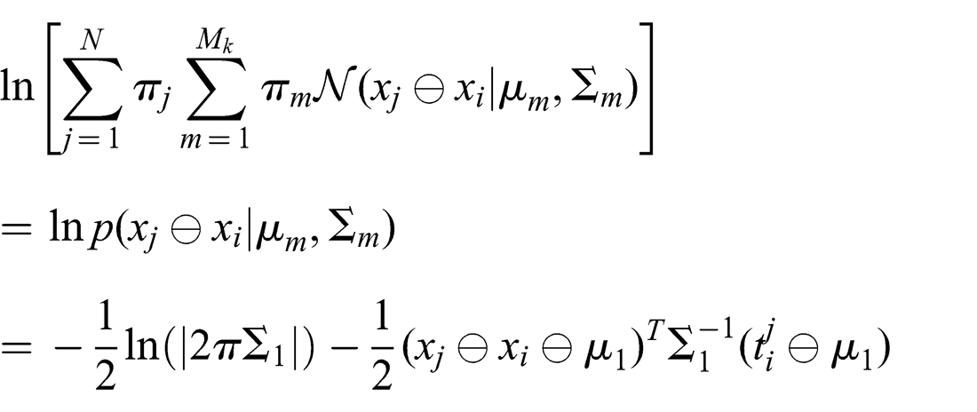
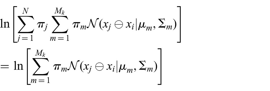
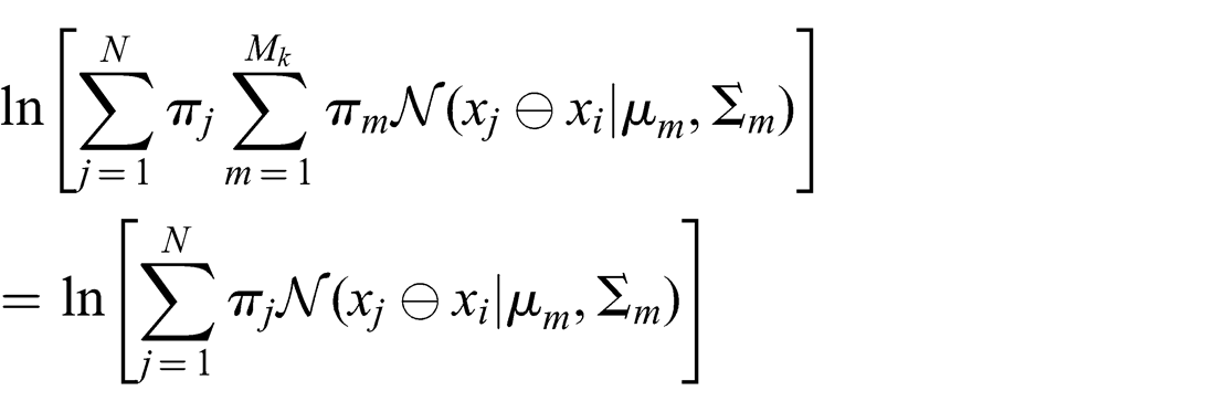
The special case where N = 1 and c₁ is a unimodal Gaussian constraint (i.e. M_k = 1) and it corresponds to the representation in the work by Sunderhauf and Protzel (2012b). In this case, π₁ = ω_ij = sig(s_ij), where s_ij is the switch variable between vertices v_i and v_j (see equation (7) in Sunderhauf and Protzel (2012b)). Similarly, the RRR algorithm of Latif et al. (2012a,b) makes a strictly binary decision where Sunderhauf and Protzel (2012b) make a fuzzy one, and its graph representation can thus be modeled the same way in this framework.

The representation in the Max-Mixture method (see Olson and Agarwal (2012, 2013)) can be thought of as the special case where the weights π_j and π_m are adjusted at every iteration such that only one of π_j and π_m retains its original value

$$(j*,m*)=\underset{j,m}{\mathrm{argmax}}{\pi }_j{\pi }_{m}p(\mathrm{dx}|{\mu }_m,{\Sigma }_m)$$

(13)

$${\pi }_j=\{\begin{array}{cc}\hfill {\pi }_j\hfill & \hfill \mathrm{if}j=j*\hfill \\ \multicolumn{1}{c}{0}& \hfill \mathrm{otherwise}\hfill \end{array}$$

(14)

$${\pi }_m=\{\begin{array}{cc}\hfill {\pi }_m\hfill & \hfill \mathrm{if}m=m*\hfill \\ \multicolumn{1}{c}{0}& \hfill \mathrm{otherwise}\hfill \end{array}$$

(15)

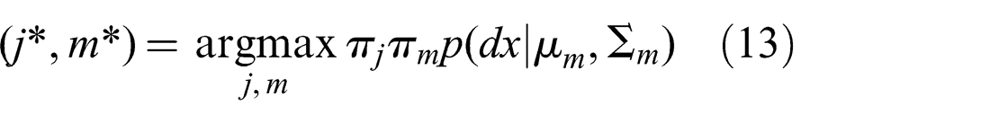
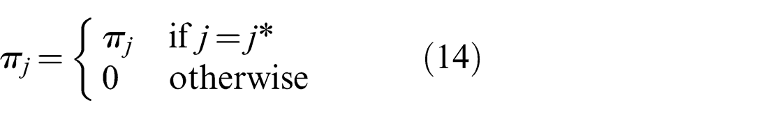
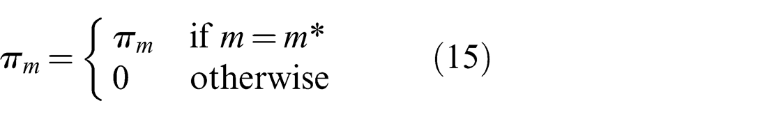
Olson and Agarwal (2012, 2013) aggregate the two conceptually separate weights π_j and π_m into one weight in their discussion, as in the equivalent formulation presented in equation (12). As such, they do not offer an implicit Null hypothesis choice, but the mixture has to explicitly include a normal distribution defined to be the Null hypothesis, which usually has a very large covariance.

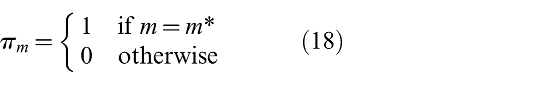
The optimization in the Generalized Graph SLAM framework described in the next section is used to make a similar selection of weights as Max-Mixture does, but in a dedicated discrete optimization stage preceding the continuous least-squares optimization. In addition, weights are set such that exactly one π_j and one π_m per edge is equal to one, indicating the component that best explains the estimate generated by the Prefilter method

$$(j*,m*)=\underset{j,m}{\mathrm{argmax}}{\pi }_j{\pi }_{m}p(\mathrm{dx}|{\mu }_m,{\Sigma }_m)$$

(16)

$${\pi }_j=\{\begin{array}{cc}\hfill 1\hfill & \hfill \mathrm{if}j=j*\hfill \\ \multicolumn{1}{c}{0}& \hfill \mathrm{otherwise}\hfill \end{array}$$

(17)

$${\pi }_m=\{\begin{array}{cc}\hfill 1\hfill & \hfill \mathrm{if}m=m*\hfill \\ \multicolumn{1}{c}{0}& \hfill \mathrm{otherwise}\hfill \end{array}$$

(18)

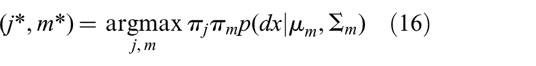
Note that the choice of j* = 0 is included, meaning that the Null hypothesis may be chosen.

4. Generalized prefilter for SLAM midstage optimization

4.1. Motivation

The previous section focused on the representational Generalized Graph SLAM framework, but made no assumptions about possible optimization methods operating on this representation. This section develops a novel optimization method suited to address all aspects of the presented framework.

The basic assumption already made in the previously introduced Prefilter method (Pfingsthorn and Birk, 2013) is that multiple components in a MoG constraint denote separate modes of the distribution and therefore shall be mutually exclusive. This assumption was motivated by encoding several distinct local optima in registration methods as also described in a more general fashion in Section 6.1.1. Again, assuming a well-behaved registration method, the basins of convergence to any of these local optima would be significant, and therefore well separated. The same assumption of mutual exclusion is extended here to hypercomponents expressing global ambiguity. The mutual exclusivity assumptions of hypercomponents and MoG components allow the formulation of a discrete optimization stage that finds or approximates the globally optimal choice of hypercomponent and MoG component per edge. Only this component is forwarded as a simple constraint to the continuous optimization backend.

4.2. The Generalized Prefilter method

The Generalized Prefilter method is introduced as a new stage between the SLAM front- and backend to perform a discrete optimization to find globally optimal component choices in a MoG hypergraph of the Generalized Graph SLAM framework. An interesting aspect of the Generalized Prefilter algorithm is that it can handle the discrete optimization of multimodal and hyperedge components in a coherent unified way. The next paragraph summarizes how the method works.

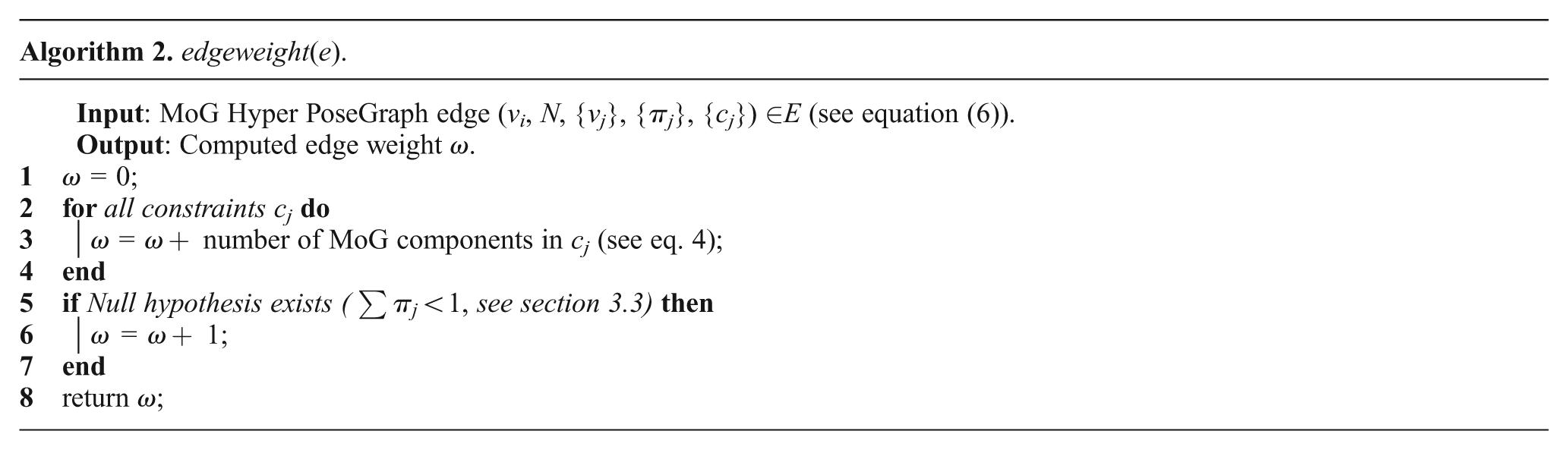
The Generalized Prefilter method uses a minimum spanning tree traversal where the edge weights are computed using the number of all MoG mixture components present in an edge, including the Null hypothesis (see Algorithm 2 and equation (6)).

Algorithm 1. The Generalized Prefilter algorithm.
Input: MoG Hyper PoseGraph G (see Section 3.3), maximum number of hypotheses N.
Output: X: A set of N sets of vertex poses X = {xi}.
1 initialize an empty list T of traversal states;
2 let (X, Vused, Eused, P) be a traversal state;
3 X = {x1};
4 Vused = {v1};
5 Eused = ∅;
6 initialize priority queue P to sort by edgeweight(e);
7 for all adjacent edges e of v1do
8  enqueue(P, (v1, e));
9  Eused = Eused∪ {e};
10 end
11 append (X, Vused, Eused, P) to T;
12 while there is a (X, Vused, Eused, P) ∈T where¬empty(P) and |t.Vused| < |V| do
13  for (X, Vused, Eused, P) ∈T where¬empty(t.P) and |t.Vused| < |V| do
14   (v, e = (vi, N, {vj}, {πj}, {cj})) = dequeue(P);
15   if v = vithen
16    for every hyperedge component jdo
17     ExpandMultimodal(T, (X, Vused, Eused, P), v, vj, cj);
18    end
19   else
20    let j be the hyperedge component where vj = v;
21    ExpandMultimodal(T, (X, Vused, Eused, P), vj, v, invert(cj));
22   end
23   if $\sum _{j=1}^N{\pi }_j=1$ then
24    remove the current tree state (X, Vused, Eused, P) from T;
25   end
26  end
27  if |T| > Nthen
28   sort T by joint probability (eq. 10) of assigned vertex poses X of each element;
29   truncate T to contain only the N most probable elements;
30  end
31 end
32  $\mathbf{X}=\bigcup _{(\mathbf{X},V_{\mathrm{used}},E_{\mathrm{used}},P)\in \mathbf{T}}\mathbf{X};$

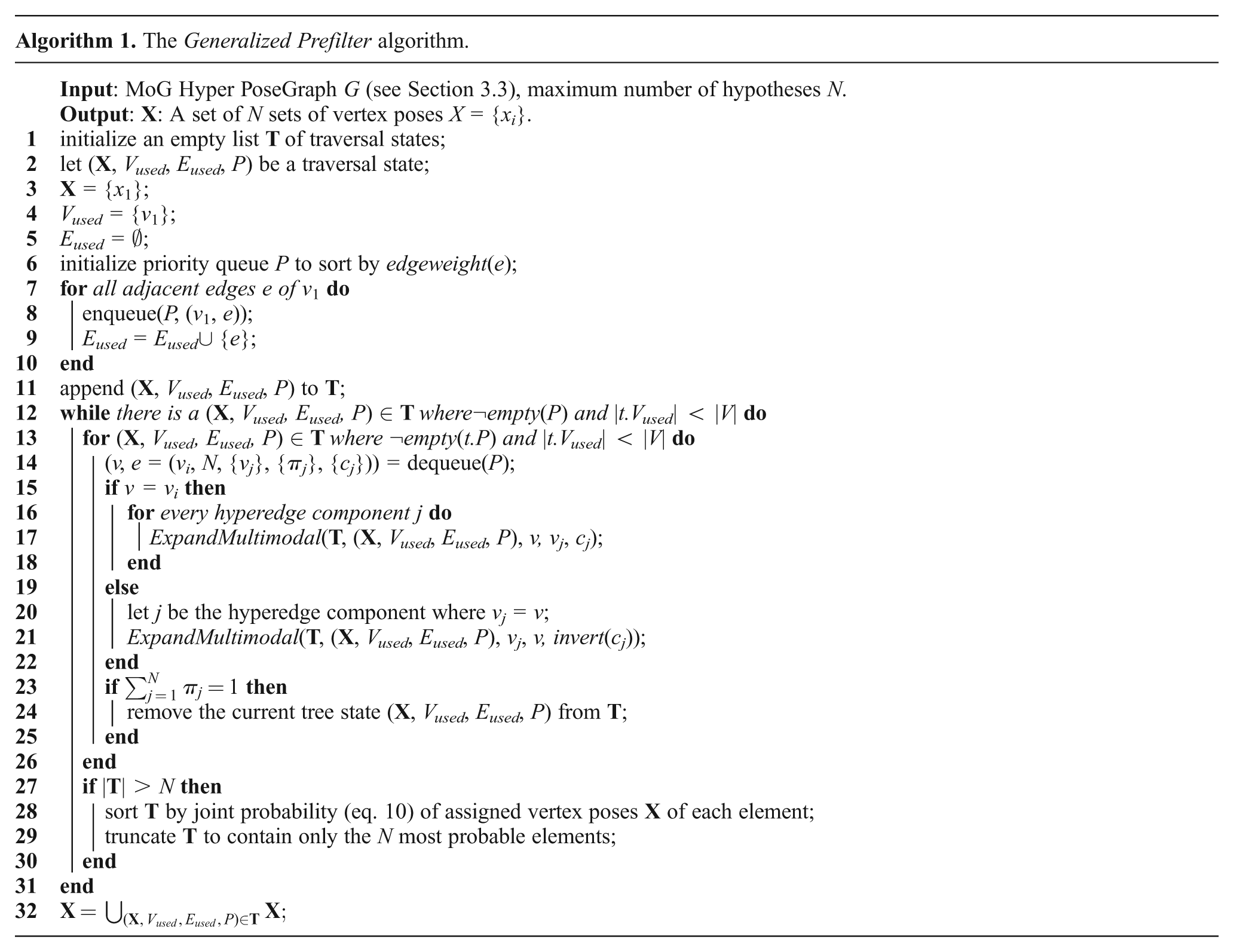
Therefore it is a minimum ambiguity spanning tree traversal of the MoG hypergraph. During this traversal, a combinatorial tree is generated with each level in the tree corresponding to an iteration of the traversal, and each node representing the exact component (including the Null hypothesis choice for hyperedges) chosen in the traversal. Each component carries relative pose information, which is used to assign poses to vertices visited in the traversal. This combinatorial tree is searched using beam search, where only the best N leafs, i.e. the ones with the highest joint probability given the computed pose estimates, are kept at each iteration of the hypergraph traversal. When the traversal completes, the best leaf, and thus the component choices along the corresponding hypergraph traversal, is picked, the computed poses in this leaf are assigned to the vertices in the graph, and the remaining ambiguous edges are disambiguated by picking the component that best explains the computed pose estimates of the related vertices. Finally, this disambiguated unimodal graph including the computed vertex poses is returned from this new SLAM midstage and it can be further processed with a standard continuous optimization method in a state-of-the-art SLAM backend.

Algorithm 2. edgeweight(e).
Input: MoG Hyper PoseGraph edge (vi, N, {vj}, {πj}, {cj}) ∈E (see equation (6)).
Output: Computed edge weight ω.
1 ω = 0;
2 for all constraints cjdo
3  ω = ω+ number of MoG components in cj (see eq. 4);
4 end
5 if Null hypothesis exists ( $\sum {\pi }_j<1$ , see section 3.3)then
6  ω = ω+ 1;
7 end
8 return ω;

Algorithm 1 shows the pseudocode for the Generalized Prefilter method extended to hypergraphs. The main difference to the previous MoG-only Prefilter algorithm is that through choosing the hypercomponent to follow, the underlying graph topology for each sample changes. Therefore, the state of the whole minimum spanning tree traversal has to be kept associated with the corresponding pose sample in a list of traversal state T, representing a leaf in the combinatorial search tree as described above. For simplicity, each MoG component also gives rise to a new traversal state instance, even though they do not change the graph topology and some data is duplicated.

Algorithm 3. ExpandMultimodal(T, (X, Vused, Eused, P), v, vnext, c).
Input: List of traversal states T, current traversal state (X, Vused, Eused, P), current vertex v, next vertex vnext, multimodal constraint c
Output: Modified list of traversal states T
1 for every component m in c (see eq. 4)do
2  let $(\mathbf{X}\prime ,V{\prime }_{\mathrm{used}},E{\prime }_{\mathrm{used}},P\prime )$ be a copy of the input traversal state;
3  x = pose of v in X;
4  X′ = X′∪ {x⊕μm};
5   $V{\prime }_{\mathrm{used}}=V{\prime }_{\mathrm{used}}\cup \{v_{\mathrm{next}}\}$ ;
6  for every edge eadj adjacent to vnext that is not in $E{\prime }_{\mathrm{used}}$ do
7   enqueue(P′, (vnext, eadj));
8    $E{\prime }_{\mathrm{used}}=E{\prime }_{\mathrm{used}}\cup \{e_{\mathrm{adj}}\}$ ;
9  end
10  append $(\mathbf{X}\prime ,V{\prime }_{\mathrm{used}},E{\prime }_{\mathrm{used}},P\prime )$ to T;
11 end

Note that the Null hypothesis is never directly referenced in the algorithm, or in the representation (cf. Section 3.3). By design of the algorithm, keeping an unmodified version of the current traversal state t in the list T corresponds to the case where the current edge e is not used, i.e. where the Null hypothesis is chosen. This works since edges are marked as used when they are enqueued in the priority queues, and dequeueing an edge from t without using it effectively deletes it from the graph topology for t. Furthermore, calling ExpandMultimodal(…) does not change the passed current traversal state, only new traversal states are generated corresponding to all modes. This means that by line 23 in Algorithm 1, the current traversal state t is unchanged, and thus corresponds to the Null hypothesis. Line 23 checks if the Null hypothesis is inadmissible by checking its weight, and if it is not, removes t from T, thus not following the Null hypothesis.

Figure 4 shows an example of the traversal stage of Generalized Prefilter on the graph from Figure 3. The combinatorial search tree is shown with each node in the tree showing the progression of the minimum spanning tree traversal given the component decisions (including the choice of the Null hypothesis) in its parents.

Fig. 3.

An example graph used for the detailed search tree rendering in Figure 4. Edge label denotes the number of MoG components, and hyperedges are marked with ovals. Vertices are labeled for ease of referencing in the text, vertex 0 is the root of the search tree.

The example graph contains six vertices (labeled 0 through 5; 0 being the root or start vertex) and seven edges. The edge labels show how many MoG components are present, and ovals connect MoG components of hyperedges. Thus, the graph contains three simple unimodal edges, two multimodal MoG edges and two hyperedges (one from 5 to 0, and one from 4 to both 1 and 2). For the sake of illustration, it is assumed here that the hyperedges have a non-zero Null hypothesis weight.

The example in Figure 4 is divided into columns that represent one iteration of the large while-loop (see line 12), starting with the state before the first iteration on the left. The for-loop (line 13) iterates through all traversal states t ∈ T, denoted by rounded boxes, top to bottom in one column in the diagram. Thus, |T| = 1 before the first iteration of the while-loop, and |T| = 8 in the last iteration, without pruning of the search tree. The exact graph topology that has been traversed, and from which components were chosen, is shown inside each traversal state representation. As edges are expanded in each iteration, they are marked black in the diagram. Each traversal state t ∈ T contains a set of vertex poses t.X. The vertices that have been assigned poses in each iteration are marked in black on the diagram. The sorting that happens at every iteration of the while-loop was not depicted in the figure to aid readability and to show the sequence of changes to the traversal states more clearly.

Fig. 4.

Expansion of the search tree of the graph in Figure 3. Expanded edges (via Prim’s method) per traversal state (round boxes) and vertices for which poses were assigned are marked in black. Unexpanded edges and unassigned vertices are shown in gray. Pruned traversal states are shown with dashed boxes. Note that the graph topology changes when hyperedges are expanded (column 2).

Calls to ExpandMultimodal(…) result in the creation of new states, specifically in iterations 2, 3, 4 and 5. Note that the hyperedge (marked by an oval) next to the root node is expanded in the second step, giving rise to two traversal states with different topology, one where the edge was used (top), and one where it was not used (bottom). Similarly, the expansion of the edge from vertex 1 to vertex 2 with three MoG components in iteration 3 gives rise to tree traversal states, one per component. The component chosen per state is marked on the formerly multimodal edge with the letters a through c. Subsequent expansions of multimodal edges are treated similarly.

The result of Generalized Prefilter’s traversal stage at the end of the large while-loop is shown in the right-most column. At this stage, it is also clear which exact spanning tree was used per traversal state, or final leaf in the combinatorial search tree, to reach all vertices and which components were chosen along the expansion of the combinatorial search tree. Note that the very ambiguous hyperedge from 4 to 1 and 2 with a total number of components of 4 (Null hypothesis plus three MoG components across the two hypercomponents) is never used due to its high weight, which is a core element in the algorithm, as doing so would generate more traversal states and thus need more computation time and memory.

One crucial detail of the Generalized Prefilter is the pruning of traversal states and their children, meaning the pruning of a complete subtree in the combinatorial search tree, when the number of traversal states |T| exceeds the allowed maximum N. This step is related to beam search (Bisiani, 1987; Rich and Knight, 1991), which is a variant of the best-first search and breadth-first search, where only the best w search tree nodes are expanded in each iteration, and others are completely pruned. w is called the beam width, such a beam width is applied to the traversal states T and the corresponding search tree. Without such an additional heuristic, the computation can become intractable if significant ambiguities remain in the search, despite the strategy of using a minimum spanning tree with the number of components as edge weights.

In the example in Figure 4, pruned subtrees (i.e. the respective traversal states) of the search tree are shown with dashed rounded boxes. These represent the least likely states given the pose assignments at the time of pruning, thus the most promising states are preserved. Here, N = 5, which means that not more than five traversal states are kept in memory per iteration of the while-loop, and thus |T| = 5 at the end of the search. Pruned traversal states are still shown to make clear that these subtrees do exist in an exhaustive solution.

The final set of vertex poses X sorted by their joint probability, can be used to select components from a MoG as well as hyperedge components in the same comprehensive way. In an optimized implementation, this choice only has to be made for the remaining, unused edges, marked in gray in the last column of the example shown in Figure 4.

5. Systematic evaluation with synthetic data

5.1. Experiments with the box world dataset

For a systematic evaluation of Generalized Prefilter in comparison to other state-of-the-art methods a large synthetic dataset was generated. Each generated graph in this dataset consists of 128 vertices and 256 edges. The aim of the experiments is to find out how robust different methods are with respect to ambiguities in the data, so a number of pose graphs with different complexities were generated. Specifically, the complexity metric introduced by Pfingsthorn and Birk (2013) was extended to encompass hyperedges as well

$$C(G)={\log }_2\left(\underset{e\in E}{\Pi }\sum _{j=1}^N{M}_j\right)=\sum _{e\in E}{\log }_2\left(\sum _{j=1}^N{M}_j\right)$$

(19)

This way, a hyperedge with n unimodal hypercomponents has the same complexity as a hyperedge with just one hypercomponent containing a MoG constraint with n modes. Note that the Null hypothesis, should it be present, counts as a hypercomponent as well. Therefore the metric captures the fact that hypercomponents and MoG components represent different alternative spatial relations (including the option of no relation at all) between multiple nodes in the graph that can lead to a combinatorial explosion.

Table 1 shows a summary of the generated complexity classes, the distribution and number of components in the MoG constraints, and hyperedges for this dataset. The overall percentage of non-simple edges is also shown. A total of 110 graphs were generated in 11 classes with an increasing complexity, i.e. 10 graphs were generated per class. The first 7 classes only contain MoG constraints or hyperedges with two components in varying numbers. In class 3, for example, the graphs contain two MoG constraints and one hyperedge, both with two components (X = 2 in the table). Classes 9 through 11 do not add more non-simple edges but more MoG or hyperedge components.

Table 1.

The 11 complexity classes used in the experiments with synthetic data. The last column shows the percentage of edges with multiple components. In addition to the amount of edges, the amount of different components in the edges matters for the combinatorial explosion of possible spatial arrangements as measured by the C(G) metric.

		#edges with X modes/hypercomponents
#	C(G)	X=1	X=2	X=3	X=4	X=5	%
1	1	255	0/1	0	0	0	0.4
2	2	254	1/1	0	0	0	0.8
3	3	253	2/1	0	0	0	1.2
4	4	252	2/2	0	0	0	1.6
5	8	248	4/4	0	0	0	3.2
6	16	240	8/8	0	0	0	6.4
7	32	224	16/16	0	0	0	12.8
8	64	192	32/32	0	0	0	25
9	82.72	192	16/16	16/16	0	0	25
10	105.36	192	8/8	8/8	16/16	0	25
11	126.99	192	4/4	4/4	8/8	16/16	25

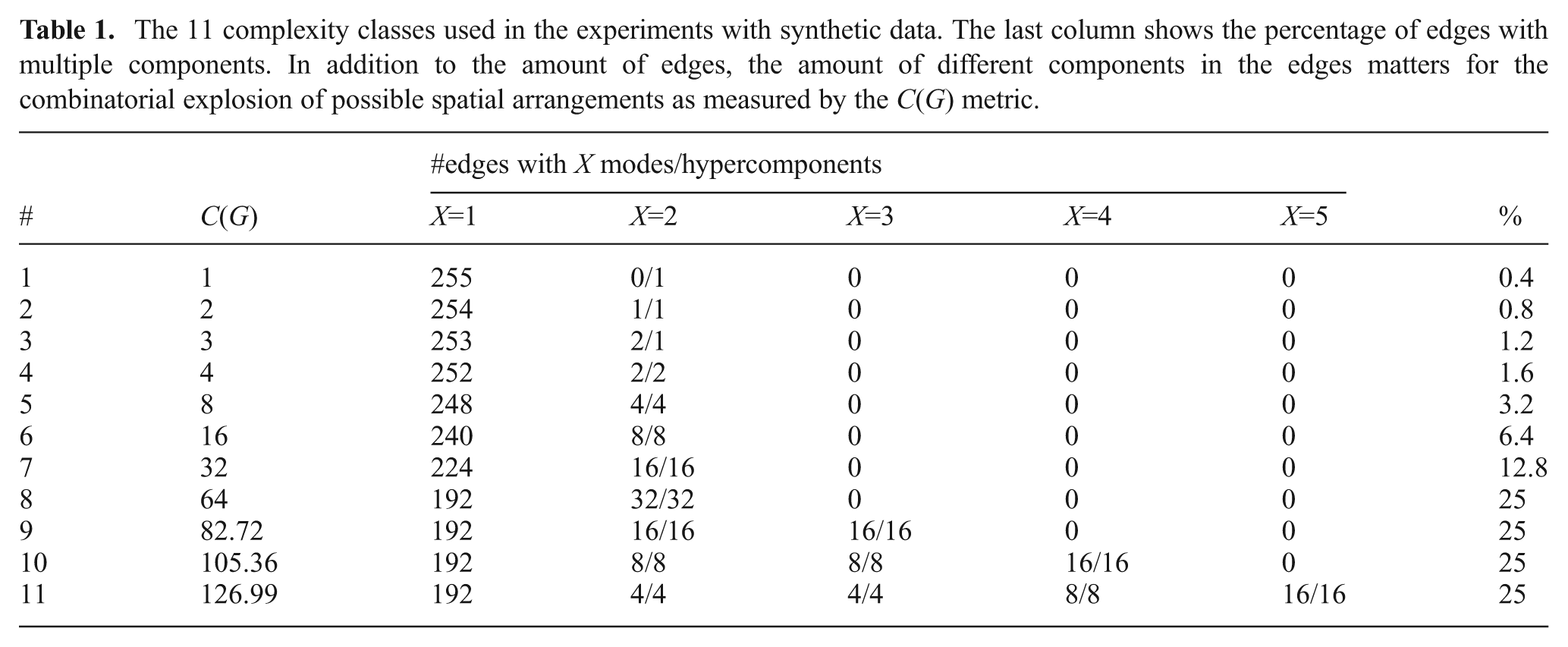
Instead of generating a completely new random graph for the more complex classes, the already generated less complex graphs were reused. Thus, a total of 10 base graphs were generated consisting completely of simple edges. For class 1, one hypercomponent was added to a random simple edge of the base graph. For class 2, one MoG component was added to a random simple edge of the same graph. For class 3, one MoG component was added to another random simple edge, and so on. For more complex classes, existing components on either hyperedges or MoG constraints were reused and additional components added where necessary. This way, the differences between the graphs in increasing complexity are minimal, and thus the performance difference of the methods is solely due to the additional components in either MoG constraints or hyperedges.

Six main methods were tested and compared. The state-of-the-art Max-Mixture (Olson and Agarwal, 2012, 2013), Switchable Constraints (Sunderhauf and Protzel, 2012a,b), Dynamic Covariance Scaling (DCS) (Agarwal et al., 2013) and RRR (Latif et al., 2012b) methods were used as a comparison basis to evaluate the Generalized Prefilter method described above. A sixth method called Max representing the traditional unimodal case (Grisetti et al., 2007a, 2010; Kaess et al., 2008; Kümmerle et al., 2011; Olson et al., 2007) where only the most likely component (hypercomponent or MoG component) is chosen, i.e. j*, m* = argmax π_jπ_m, is also used as a baseline for the other methods. Open source implementations of these methods were published by their respective authors and use the g²o library ¹ .

In contrast to the other methods that try to tackle outliers in the SLAM backend, the Generalized Prefilter is used as an additional stage between frontend and backend. Given a multimodal hypergraph, it is used to select components of all hyperedges and MoG constraints followed by a standard robust optimization implemented with the g²o library (Kümmerle et al., 2011) as the backend.

The same solver, a Gauss-Newton method implemented in g²o, was used for all approaches other than RRR, so their convergence and computational complexity can be fairly evaluated (note the GN suffix). For the Max and Generalized Prefilter methods, a Cauchy robust kernel was used with a size of 1.0, also noted in the suffix. Note also that the + sign is used in the legend to make the separation between the discrete optimization stage (Generalized Prefilter) and continuous optimization stage (Cauchy GN) clear. Naturally, any such continuous optimization stage can be used, even one of the other investigated methods like DCS GN. However, these combinations did not converge to any other solution than Generalized Prefilter+Cauchy GN, so they are neglected in this analysis. This combination will be revisited for the data discussed in Section 5.2.

The DCS GN method consequently used the DCS kernel with a kernel size (Φ) of 1.0 as recommended in Agarwal et al. (2013). Switchable Constraints implements explicit reweighting, and the Max-Mixture graph explicitly contained a Null hypothesis component, so an implicit method with a robust kernel was not used. The RRR implementation hardcoded its solver of choice, which was left as is. Each continuous optimization method (e.g. the Cauchy GN part of Generalized Prefilter) was run for 150 iterations. RRR and Generalized Prefilter ran to completion. The beam width of Generalized Prefilter was set to 300.

The difference between the investigated methods is mostly one of initialization, as any of the Max-Mixture GN, Switchable Constraints GN and DCS GN methods converge if the initial guess from the Generalized Prefilter method was used as mentioned above.

However, in order to more accurately reflect the performance on an uninitialized graph, a traditional breadth-first initialization choosing the locally most likely hypercomponent and MoG mixture component was performed before optimization with any of these methods. In fact, since Generalized Prefilter computes vertex pose estimates along with disambiguating the edge constraints, all vertex poses were set to identity before processing.

Note that all methods are run here as batch or offline methods, which is arguably the more difficult case as compared to the online case. The experiments by Olson and Agarwal (2013) focused on the online case, where the graph grows over time, but starts off small and therefore much less complex in terms of outliers, and intermediate solutions exist to bias the subsequent solutions to quickly discard new outliers.

In general, Max-Mixture GN is sensitive to the initial condition, as also noted by Olson and Agarwal (2012, 2013). The Switchable Constraints GN method is less susceptible, but still suffers significantly from bad initial conditions, as does DCS GN. RRR is supposed to be independent of the initial configuration, but often fails to maintain the connectedness of the graph.

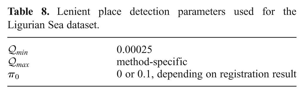
Figure 6 shows the median of the final SSE_xy and SSE_θ error (sum squared error, introduced by Olson, 2008) relative to Ground Truth of the ten sample pose graphs per complexity class after optimization using all investigated methods. Note the log scale of the y-axis. As a comparison of achievable results given the noise added to the generated graphs with Ground Truth initialization and no outliers, the final SSE errors of the optimized base graphs are also included. This optimization did not use a robust kernel, therefore it is surprising, but not impossible that the Ground Truth optimization result has a higher final error than some of the other methods. It is obvious that, even though there is a high variance for all methods, Generalized Prefilter+Cauchy GN performs multiple orders of magnitude better than Max-Mixture GN and DCS GN, and around an order of magnitude better than Switchable Constraints GN. This especially holds in highly complex conditions. Switchable Constraints GN exhibits a slightly better robustness towards graph complexity than Max-Mixture GN, though it seems to diverge much more frequently in the higher complexity conditions. DCS GN exhibits less variance than Switchable Constraints GN, but does not deal well with moderate complexity (classes 2-7), where it is outperformed by Switchable Constraints GN. Surprisingly, RRR fails at all graphs, and changing any of the exposed parameters (odometry and loop rate) has no effect. This happens because a significant number of constraints are falsely rejected, which breaks the graph (see Figure 5c).

Fig. 5.

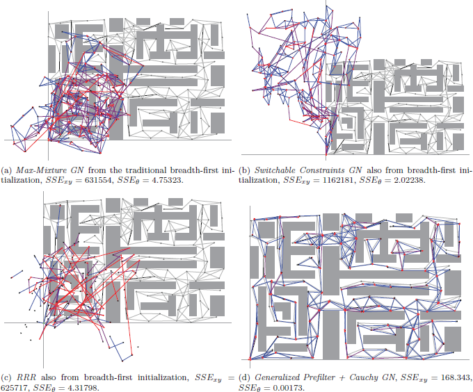
Example results of different methods on one graph of complexity class 7 with C(G) = 32. This graph has a total of 16 multimodal MoG edges with two components and 16 hyperedges with two hypercomponents. Ground truth is shown in gray in the background.

Fig. 6.

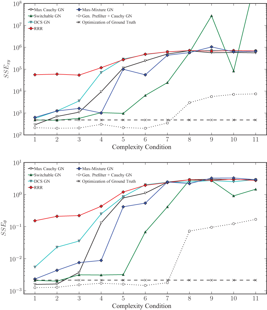
Final translation (top) and rotation (bottom) SSE metric relative to ground truth for each of the 11 complexity classes. The median values are shown. Note the log scale on the y-axes. The final SSE metric of the optimization result using the original ground truth graph is also shown for comparison. No error bars are shown for better clarity.

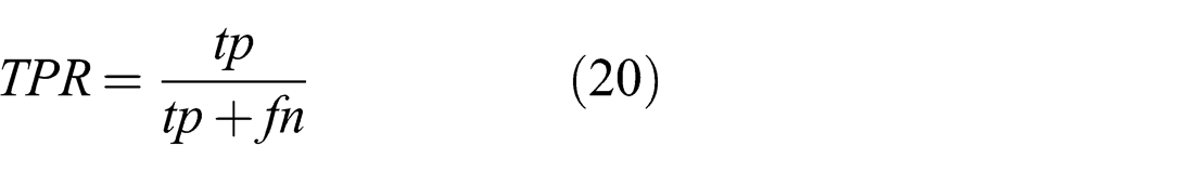
The improved performance of the Generalized Prefilter+Cauchy GN method is due to the high rate of correct choices when selecting hyperedge and MoG components. Table 2 shows the true positive rate, accuracy and average number of false positives per complexity condition. True positive rate (TPR) and accuracy (ACC) are defined as

$$\mathrm{TPR}=\frac{\mathrm{tp}}{\mathrm{tp}+\mathrm{fn}}$$

(20)

$$\mathrm{ACC}=\frac{\mathrm{tp}+\mathrm{tn}}{\mathrm{tp}+\mathrm{fp}+\mathrm{tn}+\mathrm{fn}}$$

(21)

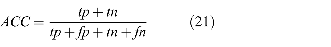
where tp is the number of true positives, fp is the number of false positives, fn is the number of false negatives and tn is the number of true negatives. The comparatively low values of TPR in conditions 3 and 4 are due to the low number of hyperedges and MoG constraints and the resulting low number of positives. In conditions 3 to 6, only a single false positive was recorded over all ten graphs.

Table 2.

True positive rate (TPR), Accuracy (ACC), and average number of false positives per graph (μ_fp) of Generalized Prefilter per complexity condition.

Cond.	1	2	3	4	5	6	7	8	9	10	11
TPR	1	1	.97	.98	.99	.99	.98	.97	.94	.94	.92
ACC	1	1	.98	.98	.99	.99	.99	.98	.97	.97	.97
μfp	0	0	.1	.1	.1	.1	.5	2.2	3.6	3.7	4.9

The main reason of failure of Max-Mixture GN, Switchable Constraints GN, DCS GN, as well as RRR on this dataset seems to be the lack of a so-called “odometry backbone”, i.e. a path of simple sequential edges that represents the robot trajectory and is generally correct. All of these methods are designed with the assumption that such a path exists, and perform very well if it is present (Sunderhauf and Protzel, 2013). Two points follow this assumption: Firstly, using this path results in an initial guess within the attraction of the global optimum. Secondly, statistical tests for outlier rejection can be executed reliably with the information on this path.

While traditional SLAM problems always display this unambiguous sequential path, this assumption is often false in cutting-edge application areas. Aerial and underwater robots are challenged by winds and currents, and mobile robots operating on rough terrain often suffer from wheel slip. Wheel slip can also occur in the most benign conditions, e.g. in an office-like environment. Such factors make outliers and ambiguities in sequential constraints hard to prevent in general, and the assumption of the existence of such an unambiguous path is very strong. In this dataset, the lack thereof is by design, as the experiments are to investigate the robustness of Generalized Prefilter and the other methods in exactly such conditions. The multimodal hypergraph representation of Generalized Graph SLAM allows an elegant way to express alternative local motion estimates, e.g. if vehicle odometry and a scan-matcher deliver inconsistent results, in addition to the incorporation of outliers in loop closures. The main purpose of the Generalized Prefilter algorithm in the SLAM midstage can hence be viewed as finding a good initial guess for the subsequent optimization in a traditional SLAM backend. This is a highly non-trivial task as the underlying problem suffers from combinatorial explosion. It is hence important to note that the heuristics of a spanning tree with edge complexity as weights and a subsequent beam search can still solve the underlying discrete optimization problem under very high amounts of local and global ambiguities.

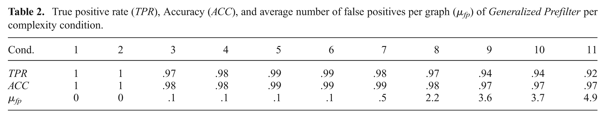
Figure 7 shows the runtimes of the compared methods. Again, note the log scale of the y-axis. The required runtime of the Max-Mixture GN method increases significantly with the graph complexity. A similar trend is evident in the time required by the Switchable Constraints GN method; note the large median runtime. The increase is less for the DCS GN method, though also pronounced. The Generalized Prefilter+Cauchy GN method only occasionally need more computational time with very complex graphs, indicated by the low median required time for this method even at high complexities. However, at these complexities (classes 8-11), the other methods no longer converge to satisfactory results at all.

Fig. 7.

Runtimes for each of the methods on all 11 complexity classes. The median values are shown. Times were recorded on an Intel i7-3770 3.4G Hz with 16 GB RAM. Runtimes varied from 0.01 s to 1.45 s over all methods, quartiles are between 0.03 s and 0.44 s. No error bars are shown for better clarity.

5.2. Experiments with the Sphere2500 dataset

In this section, a comparison of Generalized Prefilter with Max-Mixture, Switchable Constraints and DCS is undertaken on additional synthetic graphs using the standard Sphere2500 dataset (Kaess et al., 2012). As the name suggests, a simulated robot moves on a virtual 3D sphere in this dataset. The implementation of RRR currently does not support 3D graphs, thus it was not evaluated for this dataset.

The dataset has been used for the study of robust SLAM before (Agarwal et al., 2013; Olson and Agarwal, 2013; Sunderhauf and Protzel, 2012a,b). Concretely, it is used to study uncertain loop hypotheses, i.e. data only exhibiting global ambiguity, by randomly adding outlier loop constraints. Local ambiguities in the form of MoG constraints are not added for the first experiment. This is an important comparison point with the other methods, since they have been designed to address exactly and only the problem of incorrect loop hypotheses. Note that this dataset therefore contains the above mentioned “odometry backbone”, meaning unambiguous outlier-free sequential constraints, that is explicitly not required by Generalized Prefilter but is assumed to exist by other methods. While it is usually present in traditional SLAM datasets, cutting-edge SLAM applications in unstructured or harsh environments make its existence less likely as argued in the introduction. In the special case of this dataset, the investigated robust methods and Generalized Prefilter perform similarly.

However, Generalized Prefilter is designed to address both local and global ambiguity equally, a trait not shared by any other method. Additional experiments using the Sphere2500 dataset with minimal local ambiguity show the continuing robustness of Generalized Prefilter while other methods fail.

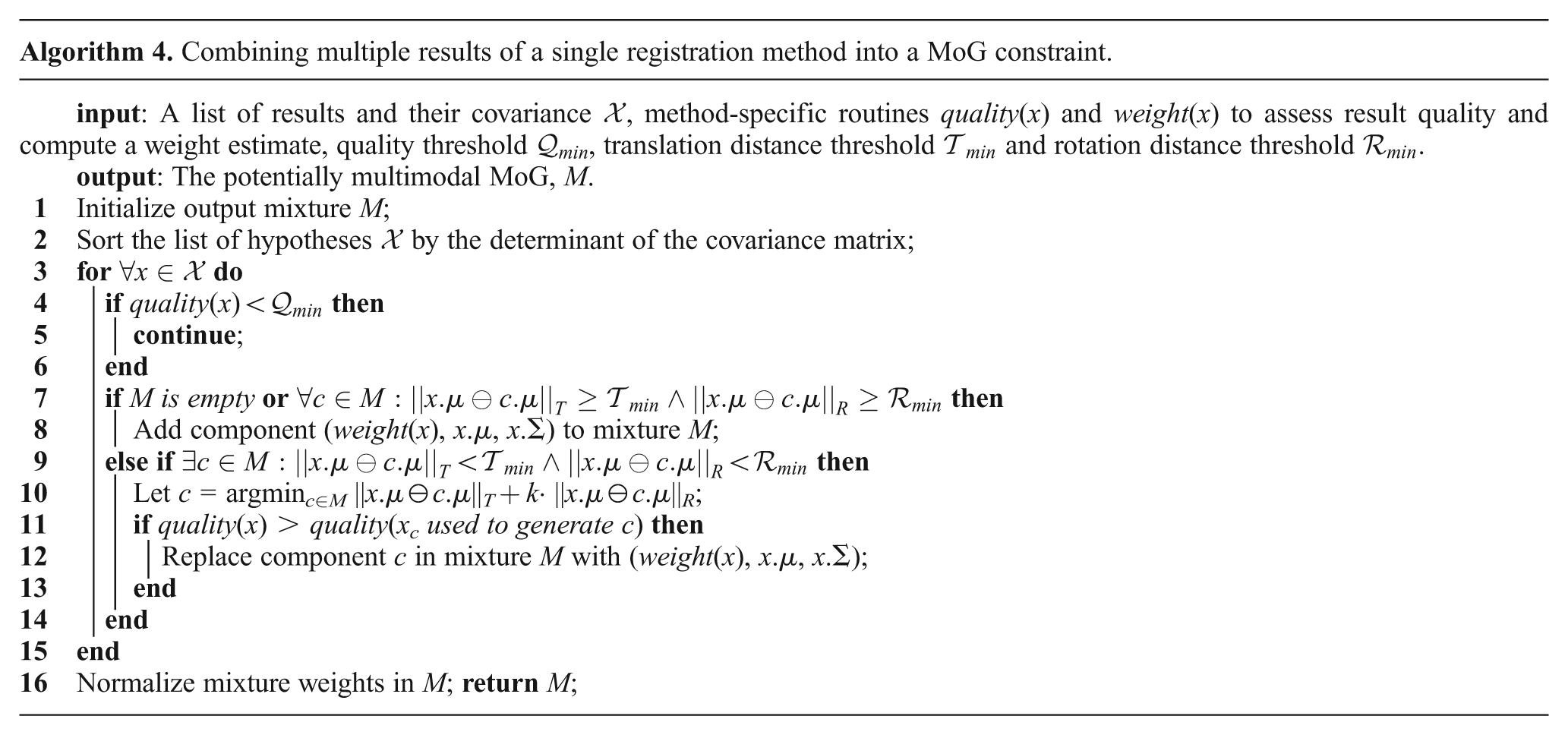
Global ambiguity is added to the original outlier-free dataset by generating a total of eight different numbers of outlier loop hypotheses, from 50 to 1000, with 40 trials each. Additional loops, represented as hyperedges with a Null hypothesis and a single simple hypercomponent, were added according the four policies by Sünderhauf (2012), each contributing to ten of the trials.

1. Random: Any two previously unconnected vertices are potential loop candidates.

2. Local: Only two previously unconnected vertices within some sequential distance to each other are candidates (e.g. with a neighborhood k, v_n may be randomly connected to any other vertex between v_n−k and v_n+k).

3. Grouped: After any two randomly connected vertices, l more vertices are connected as well (e.g. if v_i and v_j are randomly connected, so are v_i+1 and v_j+1, etc, up to v_i+l and v_j+l).

4. Locally Grouped: A combination of local and grouped above, where v_i and v_j are at most k apart.

No matter if they were randomly generated as outliers or not, all loops are treated as hyperedges, i.e. a Null hypothesis was added. This is also in line with the methodology used by Olson and Agarwal (2012, 2013) for this dataset. Note that this is an extreme case for Generalized Prefilter and the Generalized Graph SLAM framework: These generated graphs contain no local ambiguity and only global ambiguity in the form of a binary choice for each loop constraint. The unimodal loop constraint is either correct or not correct (i.e. the Null hypothesis is correct). The Generalized Graph SLAM framework representation as well as Generalized Prefilter covers a much larger set of problems, specifically including local ambiguity and global ambiguity with a variable number of choices. Such cases are evident in real world datasets where a) not all loop constraints are necessarily globally ambiguous (e.g. in the Ligurian Sea data, Section 8) and b) ambiguous loop constraints are usually much more complex (e.g. in the Bremen City data, Section 7). This specific arrangement is solely used to compare to other robust SLAM methods.

All methods other than Generalized Prefilter are initialized by sequential constraints only. Again, all vertex poses were set to zero before processing with Generalized Prefilter. Also, all methods use the general Gauss Newton algorithm with a Cholmod-based solver from the g²o library (Kümmerle et al., 2011). This is signified by the suffix GN. Since Generalized Prefilter is a discrete optimization midstage, it needs to be followed by a continuous optimization backend. Two different options are investigated here. Firstly, the Cauchy robust kernel is used for the subsequent continuous optimization, signified by the suffix Cauchy GN. Secondly, Generalized Prefilter is followed by DCS GN as backend. The + sign is used to make the separation between the discrete optimization stage (Generalized Prefilter) and continuous optimization stage (Cauchy GN/DCS GN) clear. Each optimization method was run for 20 iterations. Generalized Prefilter itself ran to completion on the input graphs with a beam width of 300.

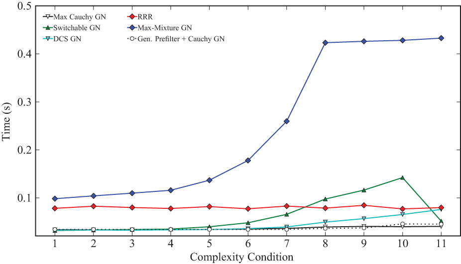
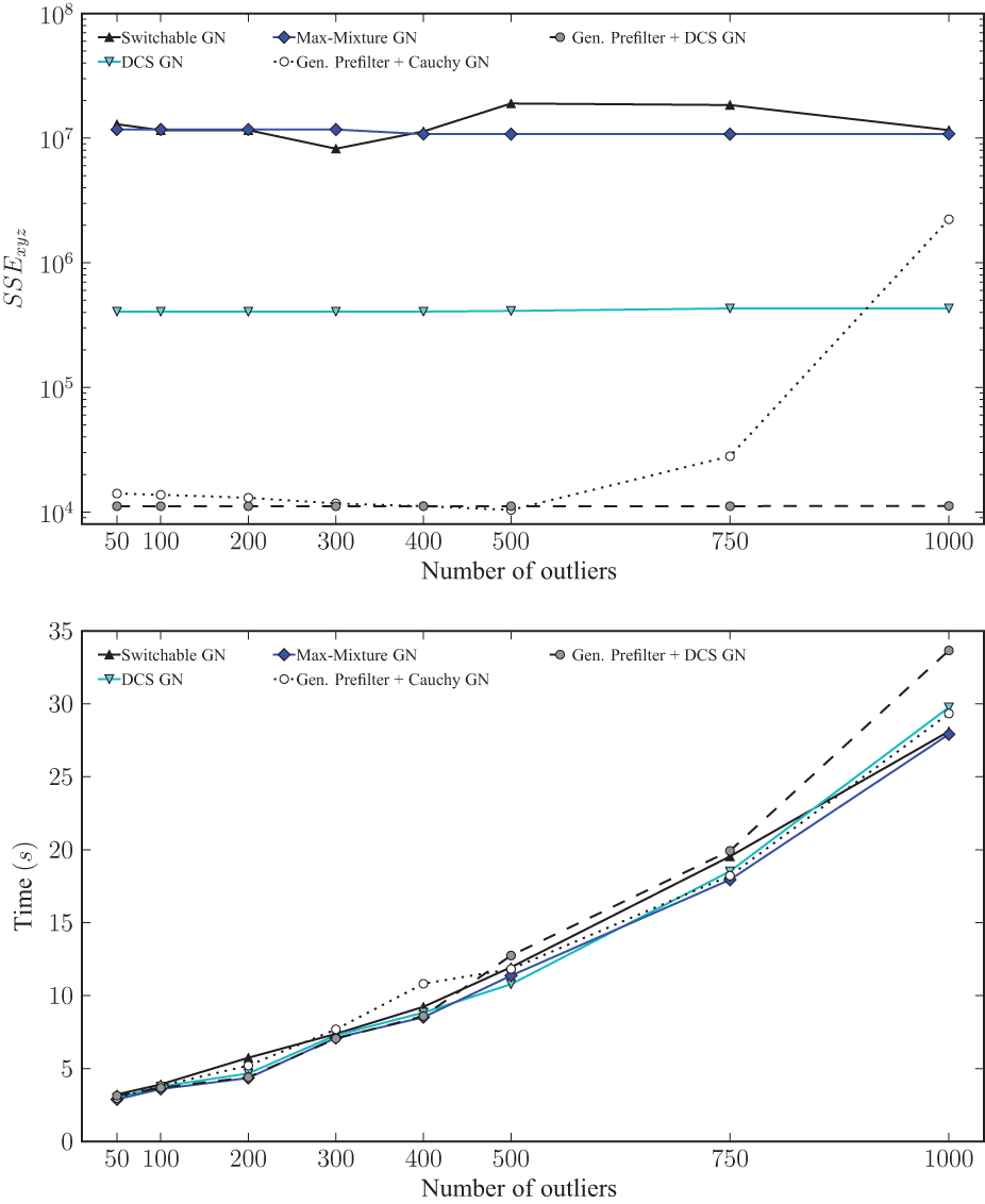
As the results in Figure 8 show, the best performing methods are DCS GN and Max-Mixture GN. Switchable Constraints GN shows somewhat more residual error. Generalized Prefilter+Cauchy GN maintains very small error in the lower number of outliers, while the error increases significantly with 750 and 1000 outliers. This is not surprising, all loops in this dataset are treated as hyperedges, therefore the sequential edges are always chosen for the minimum ambiguity spanning tree traversal. Hence, the initialization computed by Generalized Prefilter is the same as the sequential initialization already applied to the other methods, and no significant difference relative to the performance of only using a good M-estimator or robust kernel is recorded. In fact, since no ambiguity exists at all in the minimum ambiguity spanning tree, the discrete optimization step is trivial and does not require any substantial computation time. This can be observed in the time comparison in the bottom plot of Figure 8. Since no loop hypothesis was rejected by Generalized Prefilter due to a high threshold and high χ² of all loops (inliers as well as outliers) given the sequential initialization, the performance in terms of residual error as well as computation time shown here is purely that of robust regression with Gauss Newton and the Cauchy kernel. The Generalized Prefilter+DCS GN combination accordingly performs in this case much like DCS GN, i.e. it leads to very good results in all cases. Thus, all investigated robust methods perform well.

Fig. 8.

Final median translation SSE metric relative to the ground truth (top) and median runtimes (bottom) for each applicable method per number of generated outliers on the Sphere2500 dataset. The data points of DCS GN and Max-Mixture GN are hidden behind Gen. Prefilter + DCS GN in the SSE plot. Note the log scale on the y-axis of the same plot.

As mentioned before, this experiment is an extreme case for Generalized Graph SLAM and Generalized Prefilter, where only binary global ambiguities occurred.

While Generalized Prefilter in combination with DCS as robust backend still performs very well in this case, Generalized Prefilter is most effective when applied to problems with both local and global ambiguity. Therefore, two additional experiments were run to illustrate the robustness of all methods against this kind of outlier. The changes made to the data set as generated for the first experiment were minimal. For the first experiment, a single additional MoG component was added to a single sequential edge in the dataset used before, thus forming a 2-component MoG constraint. For the second experiment, another single additional MoG component was added to a different sequential edge in the same way. Thus, the second experiment contained two sequential 2-component MoG constraints.

Figures 9 and 10 show results of these two experiments. Note that even a single MoG constraint significantly diminishes the performance of other methods, while Generalized Prefilter retains the same performance (independent of the specific backend that is used). This degradation of the other methods is due to a bad initialization even when using only sequential edges due to the 2-component MoG constraints. This is also not surprising: Generalized Prefilter is designed to handle this situation where local and global ambiguity occur simultaneously and it is able to recover the original true sequential initialization in most cases, less so with many additional outliers in loop constraints (see performance difference of Generalized Prefilter+DCS GN in Figures 8 and 10). This is most likely due to some sequential outliers being congruent with loop outliers by chance. Note that this is still an extreme case for Generalized Prefilter due to the low amount of complexity in the minimum ambiguous spanning tree, this is still a rather simple problem. A total beam width of 2 and 4 would have sufficed to keep track of all possible combinations of components for these two experiments. This is not the case for the experiment described in Section 5.1.

Fig. 9.

Results of the same experiment as in Figure 8, but with a single 2-component MoG constraint in the sequential edges. The upper plot shows the final median SSE error relative to the ground truth while the lower plot shows median runtimes for each applicable method per number of generated outliers. Note the log scale on the y-axis of the SSE plot.

Fig. 10.

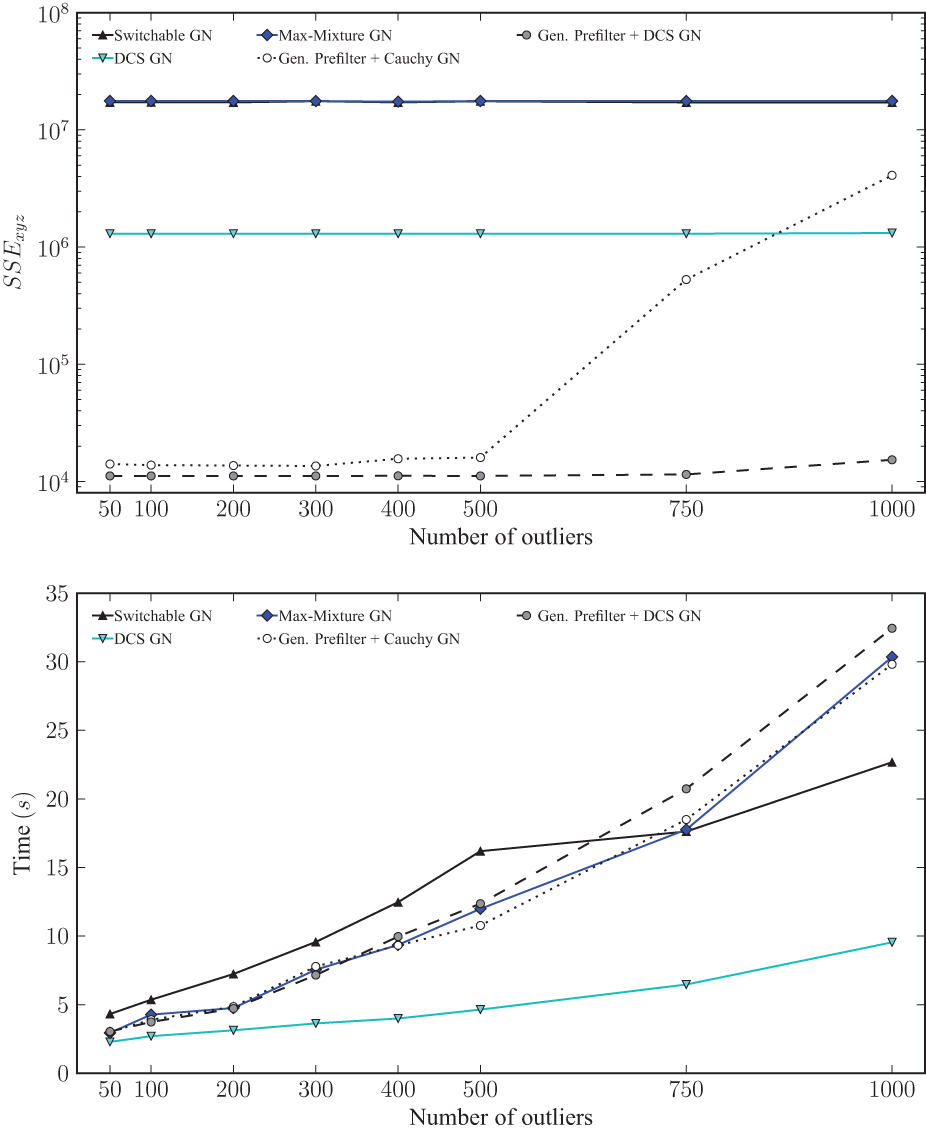
Results of the same experiment as in Figure 8, but with two 2-component MoG constraint in the sequential edges. The upper plot shows the final median SSE error relative to the ground truth while the lower plot shows median runtimes for each applicable method per number of generated outliers. Note the log scale on the y axis of the SSE plot.

The important message from these additional experiments is that methods other than Generalized Prefilter can not handle even very small amounts of local ambiguity. One or two occurrences of the least complex local ambiguity case over 2499 sequential constraints is very infrequent, yet it is enough to severely degrade the performance of other methods.

The performance difference of Generalized Prefilter+Cauchy GN and Generalized Prefilter+DCS GN shows that the choice of robust backend following Generalized Prefilter is quite important as well. As Table 2 indicates, Generalized Prefilter is an extremely efficient heuristic to deal with both local and global ambiguities, but it is not absolutely perfect. While removing almost all outliers there is always the possibility that a few remain. The more robust the final continuous optimization step used after Generalized Prefilter, the better the final result. The combination of Generalized Prefilter as discrete optimization midstage with DCS as a robust kernel for the final continuous optimization stage is an example of choosing the best of both worlds. Accordingly, Generalized Prefilter+DCS GN perform significantly better than all other methods under both local and global ambiguity, even with 1000 outliers added to the graph in the experiments presented here.

6. Practical strategies to utilize Generalized Graph SLAM

Generalized Graph SLAM is further evaluated in the next two sections with real world data. In addition, the experiments presented illustrate different general heuristic strategies to create a graph within the Generalized Graph SLAM framework. These are of interest as the main ideas can also be applied to very different SLAM applications. Therefore, a slightly more general description of the different underlying strategies is given in the rest of this section before the real world experiments and results achieved using these principles are described in Sections 7 and 8.

An effort was made to normalize the parameters required for all four strategies:

1. ${\mathcal{Q}}_{\min }$ : A minimum quality value, usually resulting from a registration or place detection method.

2. ${\mathcal{Q}}_{\max }$ : A maximum quality value, may be infinity.

3. ${\mathcal{T}}_{\min }$ : A minimum translation threshold.

4. ${\mathcal{R}}_{\min }$ : A minimum rotation threshold.

5. π ₀ : The weight of the Null hypothesis of a hyperedge.

For brevity, ⊖ is the pose difference operator, ||x|| _T is the translation norm of the (relative) pose x and ||x|| _R is the rotation norm.

6.1. Generating multimodal constraints

6.1.1. Ranked registration results

This strategy for generating multimodal edges has been presented before in Pfingsthorn and Birk (2013). It is recapitulated here for the sake of completeness since it is used in the Bremen 3D SLAM experiment (Section 7) together with the new strategy of exhaustive loop closures for generating hyperedges (Section 6.2.1).

Some registration techniques can generate a list of ranked results, e.g. HSM3D (Censi and Carpin, 2009), SRMR (Bülow and Birk, 2013), Spherical Harmonics (Kostelec and Rockmore, 2003, 2008), or plane-matching (Pathak et al., 2010). Instead of the winner-takes-all strategy of just using the top entry in the list, multimodal MoG constraints can be employed when the top registration results are of similar quality but spatially different. The weights used in the resulting mixture are then computed, as in the usual unimodal case, in the specific way for this registration method in the frontend.

Two steps are necessary to adapt an existing registration method to this scheme. Firstly, the ranked list of results should be preprocessed to discard duplicate results. Secondly, weights are to be computed for each result for inclusion in the mixture. A generic method to address both points is shown in Algorithm 4. It assumes that a covariance matrix is available for each registration result, as well as two routines to assess a) a registration-specific quality measure of a result, such as the number of correspondences, and b) a method-specific weight function for a specific result, e.g. a confidence measure. Usually, results with a lower number of congruent correspondences will have a small covariance, but will not necessarily be more accurate. Thus, Algorithm 4 will replace results if spatially similar results with a larger covariance but better quality measure exist. While this algorithm is simple, it has proven to be very useful in practice.

In total there are three parameters:

1. ${\mathcal{Q}}_{\min }$ : The minimum quality of the registration result to be added to the edge.

2. ${\mathcal{T}}_{\min }$ : The minimum translation distance.

3. ${\mathcal{R}}_{\min }$ : The according minimum rotation distance to assume two registration results in the list are equivalent.

${\mathcal{Q}}_{\min }$ should be set low enough to only reject outright registration failures, e.g. when very few inliers were found in RANSAC. ${\mathcal{T}}_{\min }$ and ${\mathcal{R}}_{\min }$ should be small, but large enough to allow for some replacements.

Algorithm 4. Combining multiple results of a single registration method into a MoG constraint.
input: A list of results and their covariance $\mathcal{X}$ , method-specific routines quality(x) and weight(x) to assess result quality and compute a weight estimate, quality threshold ${\mathcal{Q}}_{\min }$ , translation distance threshold ${\mathcal{T}}_{\min }$ and rotation distance threshold ${\mathcal{R}}_{\min }$ .
output: The potentially multimodal MoG, M.
1 Initialize output mixture M;
2 Sort the list of hypotheses $\mathcal{X}$ by the determinant of the covariance matrix;
3 for $\forall x\in \mathcal{X}$ do
4  if $\mathrm{quality}(x)<{\mathcal{Q}}_{\min }$ then
5   continue;
6  end
7  if M is emptyor $\forall c\in M:||x.\mu \ominus c.\mu |{|}_T\ge {\mathcal{T}}_{\min }\wedge ||x.\mu \ominus c.\mu |{|}_R\ge {\mathcal{R}}_{\min }$ then
8   Add component (weight(x), x.μ, x.Σ) to mixture M;
9  else if $\exists c\in M:||x.\mu \ominus c.\mu |{|}_T<{\mathcal{T}}_{\min }\wedge ||x.\mu \ominus c.\mu |{|}_R<{\mathcal{R}}_{\min }$ then
10   Let c = argminc∈M ||x.μ⊖c.μ|| T +k· ||x.μ⊖c.μ|| R ;
11   if quality(x) > quality(xc used to generate c) then
12    Replace component c in mixture M with (weight(x), x.μ, x.Σ);
13   end
14  end
15 end
16 Normalize mixture weights in M; return M;

6.1.2. Complementary motion estimates

The key insight exploited in this strategy is that different methods for motion estimates, e.g. two registration algorithms or registration and odometry, excel in different situations and particularly they provide independent measurements of the robot movement. Using, for example, multiple registration methods and combining their individual results into a multimodal result allows the exploit of redundancy and accounts for possibly diverging estimates.

While the approach to extend to combining an arbitrary number of registration results is straight forward, the rest of this section focuses on fusing exactly two estimates. Note that there is no assumption that the registration results are generated from the same sensor data pair, any other time-synchronized sensor data, including interoceptive sensors (e.g. wheel encoders for odometry), can be used as well. First of all, much like in the method outlined in Section 6.1.1, each registration method should provide a routine to compute a confidence in its result and one to compute a weight for the final mixture. In the case of more than two used registration methods, fused results are assigned the sum of the weights computed by the provided routines. Due to the fact that uncertainty information comes from different registration methods, the relative scales of the covariance matrices are not comparable. For example, a covariance computed from least-squares fit of feature correspondences has a finer scale than one computed from a discretized correlation-based method. This means they have to be multiplied by a scalar in order to be transformed into a shared scale space, which leads to one parameter per method that contributes registration results. Furthermore, it is necessary to decide if the provided registration results are mutually consistent. Using Mahalanobis distance is troublesome in this regard as it is not symmetric. Transformation estimates are compared with a separate threshold for the translation and rotation parts. Then, those registration results that are deemed consistent, i.e. representing the same estimated transformation, are fused by a simple Kalman update. This procedure is summarized in Algorithm 5.

There are a total of five parameters:

1. ω ₁ and ω₂: The covariance scale factors.

2. ${\mathcal{Q}}_{\min }$ : The minimum quality of the registration result to be added to the edge.

3. ${\mathcal{T}}_{\min }$ : The translation distance.

4. ${\mathcal{R}}_{\min }$ : The rotation distance under which fusion is appropriate.

ω ₁ and ω₂ may both be set to 1 if no other estimate is available. ${\mathcal{Q}}_{\min }$ should be set low enough to only reject outright registration failures, e.g. when very few inliers were found in RANSAC. Both ${\mathcal{T}}_{\min }$ and ${\mathcal{R}}_{\min }$ should be quite small in order to keep the accumulated error due to improper fusion of results low. If none of the registration results are trustworthy, i.e. have a quality below the minimum quality threshold, an empty mixture is returned, signaling failure. In any other case, a valid mixture is generated.

6.2. Generating hyperedge constraints

6.2.1. Exhaustive loop closure

For small graphs there is the option to register all sensor data with each other, i.e. to exhaustively iterate through all possible loop closures. Every successful registration from vertex v_n to nodes $v_{k_1}$ to $v_{k_m}$ then simply gives rise to a hyperedge. Note that no assumption about the registration result is made, it may be multimodal and thus the according component within the hyperedge could be multimodal. The main point is that outliers are acceptable in Generalized Graph SLAM. Thus, such an extremely naïve approach will still be useful since all positive loop closures are by definition included as well. In other words, recall will be 100%, while precision will be very small. This strategy can be thought of as an extreme example of lenient place recognition, discussed in the next section. It is discussed separately since it does not require a place detection method at all and since it represents an interesting corner case.

Algorithm 5. Combining multiple motion estimates, e.g. from complementary registration results or from registration plus odometry, into a MoG constraint
input: Registration results x1 and x2 with mean and covariance, covariance scales ω1 and ω2, method-specific routines quality(x) and weight(x) to assess result quality and compute a weight estimate, quality threshold ${\mathcal{Q}}_{\min }$ , translation distance threshold ${\mathcal{T}}_{\min }$ and rotation distance threshold ${\mathcal{R}}_{\min }$ .
output: MoG, M.
1 for every registration result xido
2  xi.Σ = ωi·xi.Σ;
3 end
4 Initialize output mixture M;
5 if ${max}_i\mathrm{weight}(x_i)<{\mathcal{Q}}_{\min }$ then
6  return M;
7 end
8 if ${min}_i\mathrm{weight}(x_i)<{\mathcal{Q}}_{\min }$ then
9   $x^{*}={\mathrm{argmax}}_{x_i}\mathrm{weight}\left(x_i\right)$ ;
10  Add component (1.0, x*.μ, x*.Σ) to mixture M;
11  return M;
12 end
13 if $||x_1.\mu \ominus x_2.\mu |{|}_T<{\mathcal{T}}_{\min }\wedge ||x_1.\mu \ominus x_2.\mu |{|}_R<{\mathcal{R}}_{\min }$ then
14  K = x2.Σ· (x1.Σ+x2.Σ)−1;
15  μ = x2.μ+K· (x1.μ−x2.μ);
16  Σ = x2.Σ−K·x1.Σ;
17  Add component (1.0, μ, Σ) to mixture M;
18 else
19  Add component (weight(x1), x1.μ, x1.Σ) to mixture M;
20  Add component (weight(x2), x2.μ, x2.Σ) to mixture M;
21 end
22 Normalize mixture weights in M;
23 return M;

Some optimizations of this naïve strategy can still be made. Specifically, two consecutive sensor observations should not be connected by a hyperedge, unless the distance between them is significant. It is assumed in this case that the two observations contain enough common data for the registration method(s) to succeed, even though the result may be multimodal. Thus, a vertex v_n will be connected to its direct predecessor v_n−1 with a simple or purely multimodal constraint. Hyperedge constraints are generated from vertex v_n to all vertices v_i before the previous one (i = 1, 2, 3, …, n − 2). Naturally, pairs for which the registration method could not generate a corresponding constraint are skipped.

A sketch of this naïve method is shown in Algorithm 6. There are a total of three parameters:

1. π ₀: The final weight of the Null hypothesis.

2. ${\mathcal{Q}}_{\min }$ : The minimum quality of the registration result to be added to the edge.

3. ${\mathcal{Q}}_{\max }$ : The maximum quality of the registration result above, in which the result is added as a single, potentially multimodal, edge instead of a component of the hyperedge.

In practice, ${\mathcal{Q}}_{\max }$ can either be infinity, adding all registration results to the hyperedge, or a value sufficiently high to only allow generation of separate simple or multimodal edges for true positives. On the other hand, ${\mathcal{Q}}_{\min }$ should be set very low, just low enough to discard cases where the registration method(s) failed completely.

6.2.2. Lenient place recognition

Place recognition methods, such as FabMAP (Cummins and Newman, 2011), usually produce multiple hypotheses. This is desirable if a given place has been visited multiple times before. On the other hand, it is possible to erroneously detect loops due to global ambiguity. Some methods even report a confidence score for each hypothesis that can be used as a mixture weight in the hyperedge.

A side benefit of having a robust optimization method that can process such hyperedge constraints is that thresholds on the confidence of loop hypotheses can be greatly reduced. While this allows more false hypotheses into the map, it also increases the number of true hypotheses. Here, the number of true and false loop hypothesis from the Ligurian Sea dataset in Section 8 is used. With a threshold of 0.99, as is custom for FabMAP, a total of 3846 true positives and 98 false positives are generated. With a threshold of 0.00025 instead of 0.99, a total of 19820 true positives and 7402 false positives are generated. Thus, it is possible to increase the number of true loop hypotheses by 15974, while only increasing false hypotheses by 7304. That is 218.7% true positives relative to false positives just by decreasing the threshold significantly.

Algorithm 6. Adding a vertex to the graph using exhaustive loop closures.
input: Multimodal Hypergraph G = (V, E), new vertex vt with associated observation zt, a registration method registration(zref, z) that returns a constraint and a quality measure, the Null hypothesis weight π0, minimum quality of registration result ${\mathcal{Q}}_{\min }$ , maximum quality of registration result ${\mathcal{Q}}_{\max }$ .
output: Extended Multimodal Hypergraph G = (V, E).
1 Add vertex vt to V;
2 (cseq, qseq) = registration(zt−1, zt);
3 if $q_{\mathrm{seq}}>{\mathcal{Q}}_{\min }$ then
4  Add new edge from vt−1 to vt with constraint cseq to E;
5 end
6 Initialize hyperedge e with reference vertex vt;
7 for $\forall v_i\in V:i<t-1$ do
8   (ci, qi) = registration(zt, zi);
9  if $q_i<{\mathcal{Q}}_{\min }$ then
10   continue;
11  end
12  if $q_i>{\mathcal{Q}}_{\max }$ then
13   Add new edge from vt to vi with constraint ci to E;
14  else
15   Add hypercomponent towards vi with weight qi and constraint ci to e;
16  end
17 end
18 if e has hypercomponentsthen
19  Normalize hypercomponent weights in e;
20  Add Null hypothesis with weight π0 to e and normalize hypercomponent weights again;
21  Add hyperedge e to E;
22 end
23 return G;

An example of the case where the best reported loop hypothesis is actually wrong is shown in Figure 11. Here, a close by but completely different area was identified as the best match with a confidence of 0.9472. The correct data is identified with a very low confidence of 0.0427082. Such potentially very informative loop hypotheses would be missed if the thresholds are kept high.

Fig. 11.

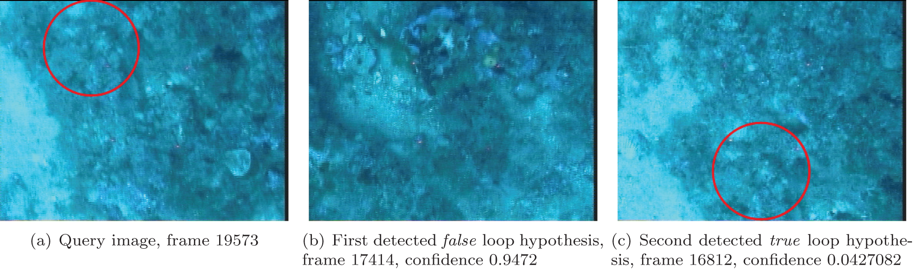
An example of a loop detection process where a highly confident result is wrong (b), and a very lowly rated result is right (c). This ambiguous loop detection would have been missed with a low threshold. Note the indicated region of common features.

Algorithm 7 shows how to use such lenient place recognition results to generate hyperedge constraints. As expected, it is very similar to that using exhaustive loop hypotheses. Instead of iterating over all older vertices, only those listed in the place recognition results are examined. The main difference is in the use of the ${\mathcal{Q}}_{\min }$ parameter, which is now applied to the place recognition results. All other parameters are the same.

Algorithm 7. Adding a vertex to the graph using lenient place detection.
input: Multimodal Hypergraph G = (V, E), new vertex vt with associated observation zt, a list of place recognition results $p\in \mathcal{P}$ , a registration method registration(zref, z) that returns a constraint and a quality measure, the Null hypothesis weight π0, minimum quality of place recognition result ${\mathcal{Q}}_{\min }$ , maximum quality of registration result ${\mathcal{Q}}_{\max }$ .
output: Extended Multimodal Hypergraph G = (V, E).
1 Add vertex vt to V;
2 (cseq, qseq) = registration(zt−1, zt);
3 if $q_{\mathrm{seq}}>{\mathcal{Q}}_{\min }$ then
4  Add new edge from vt−1 to vt with constraint cseq to E;
5 end
6 Initialize hyperedge e with reference vertex vt;
7 for $p\in \mathcal{P}$ do
8  i = p.index; qi = p.confidence;
9  if $q_i<{\mathcal{Q}}_{\min }$ then
10   continue;
11  end
12   $(c_i,q_{c_i})=\mathrm{registration}(z_t,z_i)$ ;
13  if $q_{c_i}>{\mathcal{Q}}_{\max }$ then
14   Add new edge from vt to vi with constraint ci to E;
15  else
16   Add hypercomponent towards vi with weight qi and constraint ci to e;
17  end
18 end
19 if e has hypercomponentsthen
20  Normalize hypercomponent weights in e;
21  Add Null hypothesis with weight π0 to e and normalize hypercomponent weights again;
22  Add hyperedge e to E;
23 end
24 return G;

7. 3D mapping with plane matching on the Bremen City dataset

This experiment serves two main purposes. Firstly, it provides an additional comparison of the performance of Generalized Graph SLAM to other methods but by using real data as opposed to synthetic graphs. Secondly, it illustrates the use of two strategies from Section 6, namely ranked registration results to generate multimodal constraints (Section 6.1.1) and exhaustive loop closure to generate hyperedges (Section 6.2.1).

The real world dataset for this experiment is based on 13 scans that were recorded with a Riegl VZ-400 in the center of Bremen, Germany. Each point cloud consists of between 15 and 20 million points with reflectance information. The scanner was mounted on a tripod without a mobile base, thus no odometry information is available. However, markers were placed in the environment beforehand to allow for a comparison with the “gold standard” for geodetic applications, i.e. registration with artificial markers in the Riegl software which requires additional manual assistance in the process like confirming or re-selecting correspondences. This registration based on artificial markers can also be used to seed methods that need a good initial guess, e.g. for ICP based methods like 6D-SLAM (Borrmann et al., 2008). Note that no initial guess, i.e. no initial marker based registration, no motion estimates, no GPS, or anything similar is used for the 3D plane registration.

This dataset has been used in the authors’ original article presenting the multimodal-only Prefilter method (Pfingsthorn and Birk, 2013). The same strategy for ranked registration results (Section 6.1.1) is used here again for plane-matching (Pathak et al., 2010). Algorithm 8 is repeated here from Pfingsthorn and Birk (2013) and shows the specific implementation of the strategy of ranked registration results for plane-matching. For illustration purposes, the absolute minimum overlap parameter ${\mathcal{O}}_p$ is lowered to 0.045 from 0.1, allowing even more potential registration results. This shows the robustness of Generalized Graph SLAM to deal with ambiguous registration results, due to a very lenient handling of parameters in the underlying registration method. The full set of parameters used is shown in Table 3. Note that, while Algorithm 8 performs many more thresholding operations on method-specific measures than Algorithm 4 from Section 6.1.1, it follows the same concept of quality checking sketched there.

Table 3.

Multimodal plane matching parameters used for the Bremen City dataset.

${\mathcal{O}}_p$	0.045
${\mathcal{L}}_{\mathrm{unc}}$	e 15
${\mathcal{O}}_{\min }$	0.667
${\mathcal{D}}_{\min }$	5
${\mathcal{R}}_{\min }$	0.065
λ max	800,000
${\mathcal{L}}_{\mathrm{rep}}$	e 3
${\mathcal{O}}_{\max }$	0.24
${\mathcal{D}}_{\max }$	0.2
${\mathcal{R}}_{\max }$	0.005

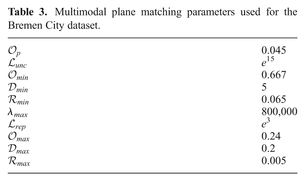
The experiment is further extended by using the exhaustive matching strategy (Section 6.2.1) to generate loop closures including hyperedges. Since the plane-matching registration method already contains very loose thresholds on the number of correspondences, no additional thresholds were applied by setting the minimum and maximum quality ${\mathcal{Q}}_{\min }$ and ${\mathcal{Q}}_{\max }$ to −∞ and ∞ respectively. This way, all reported and valid registration results are added to the hyperedge. The Null hypothesis in every hyperedge was set to have a weight of π₀ = 0.1.

Algorithm 8. Post-processing of the complete list of potential solutions $\mathcal{W}$ .
input: A list of all consistent registrations $\mathcal{W}$ from Algorithm 2 in Pathak et al. (2010).
output: The reduced list of potential solutions ${\mathcal{W}}^{*}$ .
1 Initialize ${\mathcal{W}}^{*}=\varnothing$ ;
2 Sort the elements ${\omega }_i\in \mathcal{W}$ by uncertainty volume of the solution ωi.α.
3 Set ωmin to the first ${\omega }_i\in \mathcal{W}$ where the maximum eigenvalue of ${{\omega }_i.}_r^{\ell }{\mathbf{C}}_{\stackrel{⌣}{\mathbf{q}}\stackrel{⌣}{\mathbf{q}}}$ and ${{\omega }_i.}_r^{\ell }{\mathbf{C}}_{\mathbf{tt}}$ is less than λ max .
4 if no such ωmin existsthen
5  return
6 end
7 Set ${\mathcal{W}}^{*}=\{{\omega }_{\min }\}$
8 Set ${\alpha }_{\max }={\mathcal{L}}_{\mathrm{unc}}·{\omega }_{\min }.\alpha$ .
9 Set $o_{\min }={\mathcal{O}}_{\min }·{\omega }_{\min }.o_p$ .
10 for $\forall {\omega }_i\in \mathcal{W}$ do
11  if ${\omega }_i.o_p<{\mathcal{O}}_p$ or ωi.op < ominor max eigenvalue of ${{\omega }_i.}_r^{\ell }{\mathbf{C}}_{\stackrel{⌣}{\mathbf{q}}\stackrel{⌣}{\mathbf{q}}}$ or ${{\omega }_i.}_r^{\ell }{\mathbf{C}}_{\mathbf{tt}}$  > λmaxor ωi.α > αmaxthen
12   continue
13  end
14  Set jrep = −1
15  for $\forall {\omega }_j^{*}\in {\mathcal{W}}^{*}$ do
16   if $||{\omega }_i{.}_r^{\ell }\mathbf{t}-{\omega }_j^{*}{.}_r^{\ell }\mathbf{t}||<{\mathcal{D}}_{\min }$ or ${{\omega }_i.}_r^{\ell }\stackrel{⌣}{\mathbf{q}}<{\mathcal{R}}_{\min }$ then
17    jrep = j
18    break;
19   end
20  end
21  if jrep == −1 then
22   Append ${\mathcal{W}}^{*}\leftarrow {\mathcal{W}}^{*}\cup \{{\omega }_i\}$
23  end
24  else
25   This ωi may replace ${\omega }_{j_{\mathrm{rep}}}^{*}$ .
26   if ${\omega }_i.o_p>{\omega }_{j_{\mathrm{rep}}}^{*}.o_p$ and ${\omega }_i.o_p<{\mathcal{O}}_{\max }$ and ${\omega }_i.\alpha <{\omega }_{j_{\mathrm{rep}}}^{*}.\alpha ·{\mathcal{L}}_{\mathrm{rep}}$ and $||{\omega }_i{.}_r^{\ell }\mathbf{t}-{\omega }_j^{*}{.}_r^{\ell }\mathbf{t}||<{\mathcal{D}}_{\max }$ and ${{\omega }_i.}_r^{\ell }\stackrel{⌣}{\mathbf{q}}<{\mathcal{R}}_{\max }$ then
27    Replace ${\omega }_{j_{\mathrm{rep}}}^{*}$ with ωi
28   end
29  end
30 end

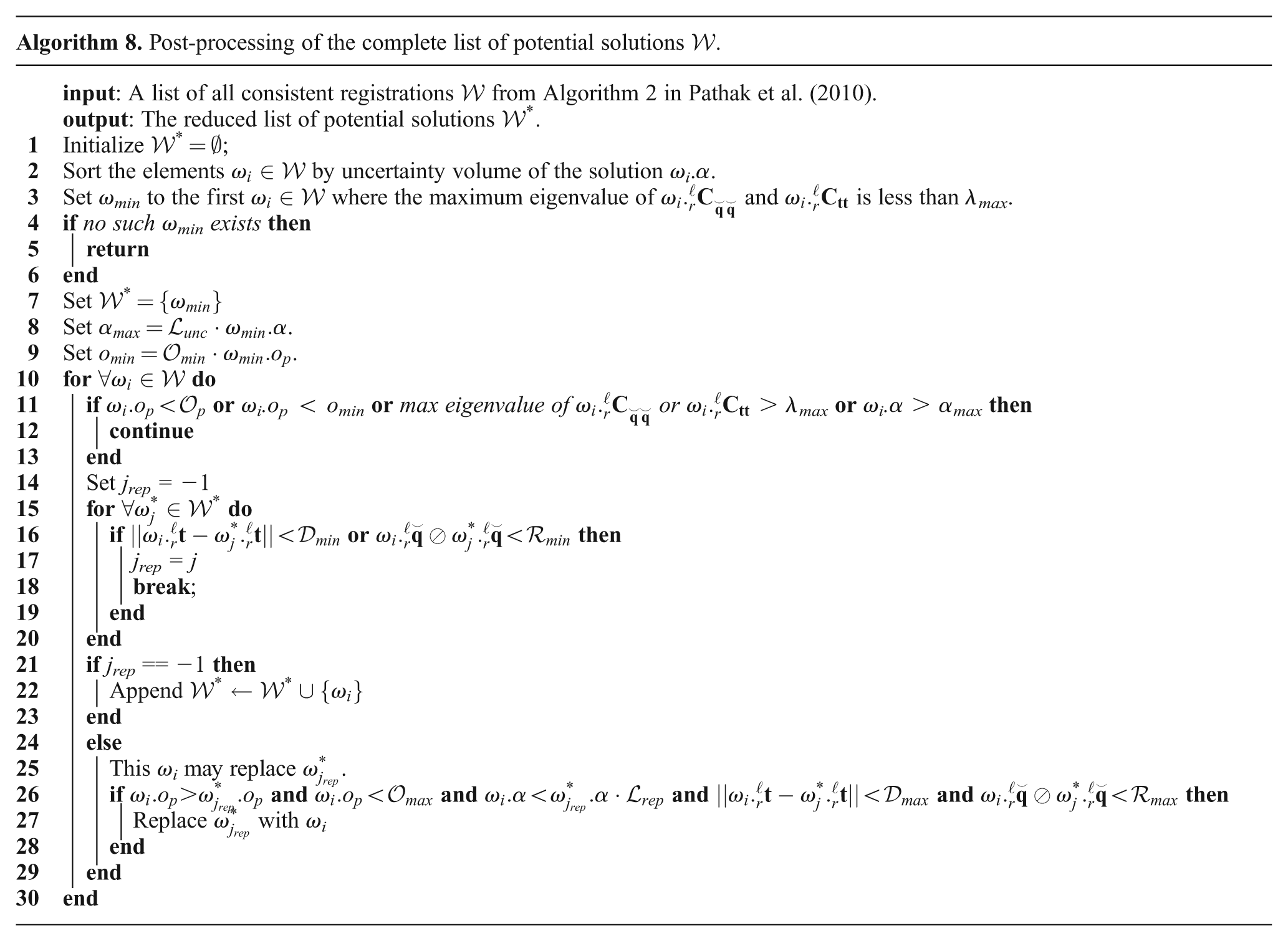
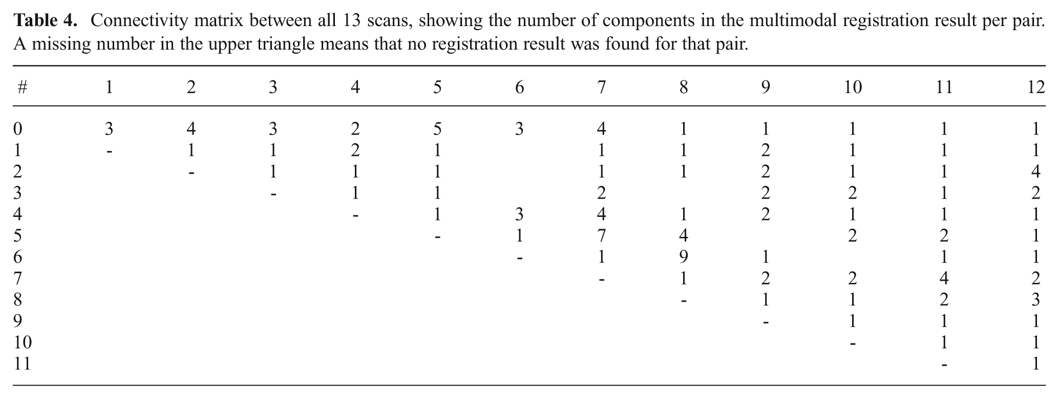
Table 4 shows a connectivity matrix between all scan pairs. Note that the graph is almost completely connected because of the exhaustive loop generation. However, there are only 23 edges in the graph. These are the 12 sequential MoG edges, and 11 non-sequential MoG hyperedges. For example, the loop closing MoG hyperedge from scan 7 to its predecessors 0 through 5 contains six hypercomponents with a total of 19 MoG components. This results in a graph complexity C(G) = 36.95, which is large regarding the small size of the graph.

Table 4.

Connectivity matrix between all 13 scans, showing the number of components in the multimodal registration result per pair. A missing number in the upper triangle means that no registration result was found for that pair.

#	1	2	3	4	5	6	7	8	9	10	11	12
0	3	4	3	2	5	3	4	1	1	1	1	1
1	-	1	1	2	1		1	1	2	1	1	1
2		-	1	1	1		1	1	2	1	1	4
3			-	1	1		2		2	2	1	2
4				-	1	3	4	1	2	1	1	1
5					-	1	7	4		2	2	1
6						-	1	9	1		1	1
7							-	1	2	2	4	2
8								-	1	1	2	3
9									-	1	1	1
10										-	1	1
11											-	1

Table 5.

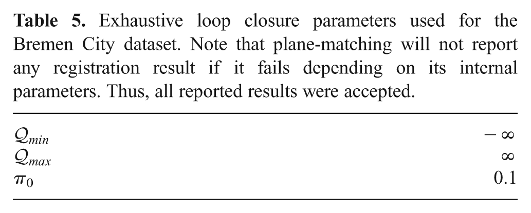
Exhaustive loop closure parameters used for the Bremen City dataset. Note that plane-matching will not report any registration result if it fails depending on its internal parameters. Thus, all reported results were accepted.

${\mathcal{Q}}_{\min }$	−∞
${\mathcal{Q}}_{\max }$	∞
π 0	0.1

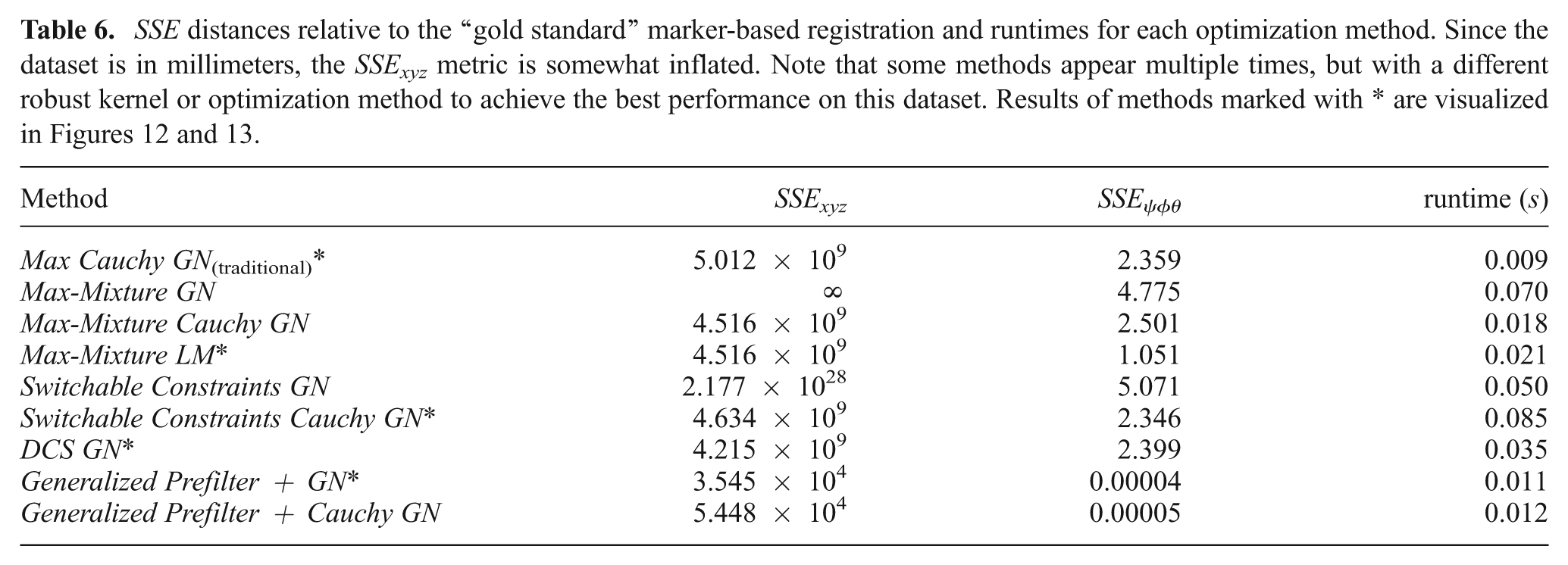
There exists a ground truth estimate for this dataset based on artificial RIEGL markers that have been placed in the environment. Table 6 shows the final SSE distances relative to the marker-based ground truth for all tested optimization methods, as well as the required computation time. The implementation of RRR by Latif et al. (2012b) currently does not support 3D pose graphs, thus it was not evaluated for this dataset. The parameters for these methods are the same as used in the evaluation with the synthetic data (Section 5) up to three exceptions: The kernel size for the Cauchy robust kernel used for the Max method was increased to 10; the Generalized Prefilter method did not use any robust kernel in the subsequent continuous optimization; the Switchable Constraints method was additionally run with the Cauchy robust kernel because the non-robust Gauss Newton algorithm did not converge; and the Max-Mixture method was additionally run with the Levenberg-Marquardt (LM) algorithm instead of Gauss Newton. Note also the same suffixes denoting the exact optimization algorithm and robust kernel used in g²o. All evaluated results that converged to some local optimum are shown in the table. Only the best achieved results (marked by * in the table) per method are visualized in Figures 12 and 13.

Table 6.

SSE distances relative to the “gold standard” marker-based registration and runtimes for each optimization method. Since the dataset is in millimeters, the SSE_xyz metric is somewhat inflated. Note that some methods appear multiple times, but with a different robust kernel or optimization method to achieve the best performance on this dataset. Results of methods marked with * are visualized in Figures 12 and 13.

Method	SSExyz	SSEψϕθ	runtime (s)
Max Cauchy GN (traditional)*	5.012 × 109	2.359	0.009
Max-Mixture GN	∞	4.775	0.070
Max-Mixture Cauchy GN	4.516 × 109	2.501	0.018
Max-Mixture LM*	4.516 × 109	1.051	0.021
Switchable Constraints GN	2.177 × 1028	5.071	0.050
Switchable Constraints Cauchy GN*	4.634 × 109	2.346	0.085
DCS GN*	4.215 × 109	2.399	0.035
Generalized Prefilter + GN*	3.545 × 104	0.00004	0.011
Generalized Prefilter + Cauchy GN	5.448 × 104	0.00005	0.012

Table 7.

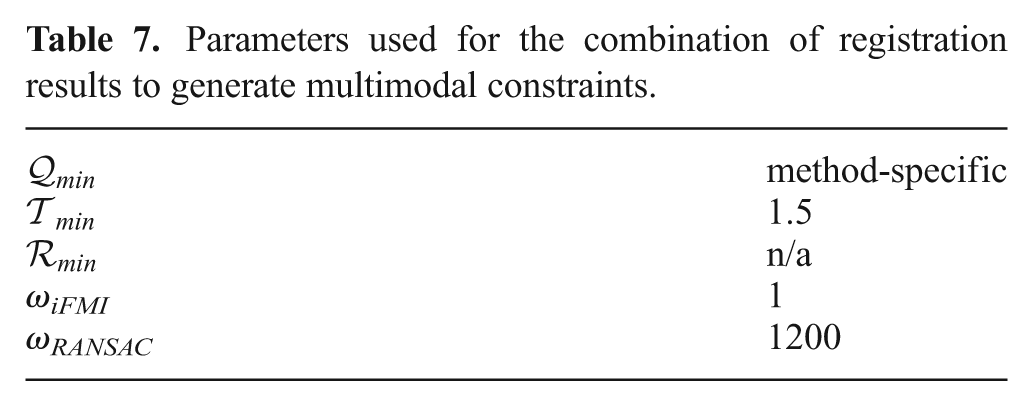
Parameters used for the combination of registration results to generate multimodal constraints.

${\mathcal{Q}}_{\min }$	method-specific
${\mathcal{T}}_{\min }$	1.5
${\mathcal{R}}_{\min }$	n/a
ωiFMI	1
ωRANSAC	1200

Table 8.

Lenient place detection parameters used for the Ligurian Sea dataset.

${\mathcal{Q}}_{\min }$	0.00025
${\mathcal{Q}}_{\max }$	method-specific
π 0	0 or 0.1, depending on registration result

Fig. 12.

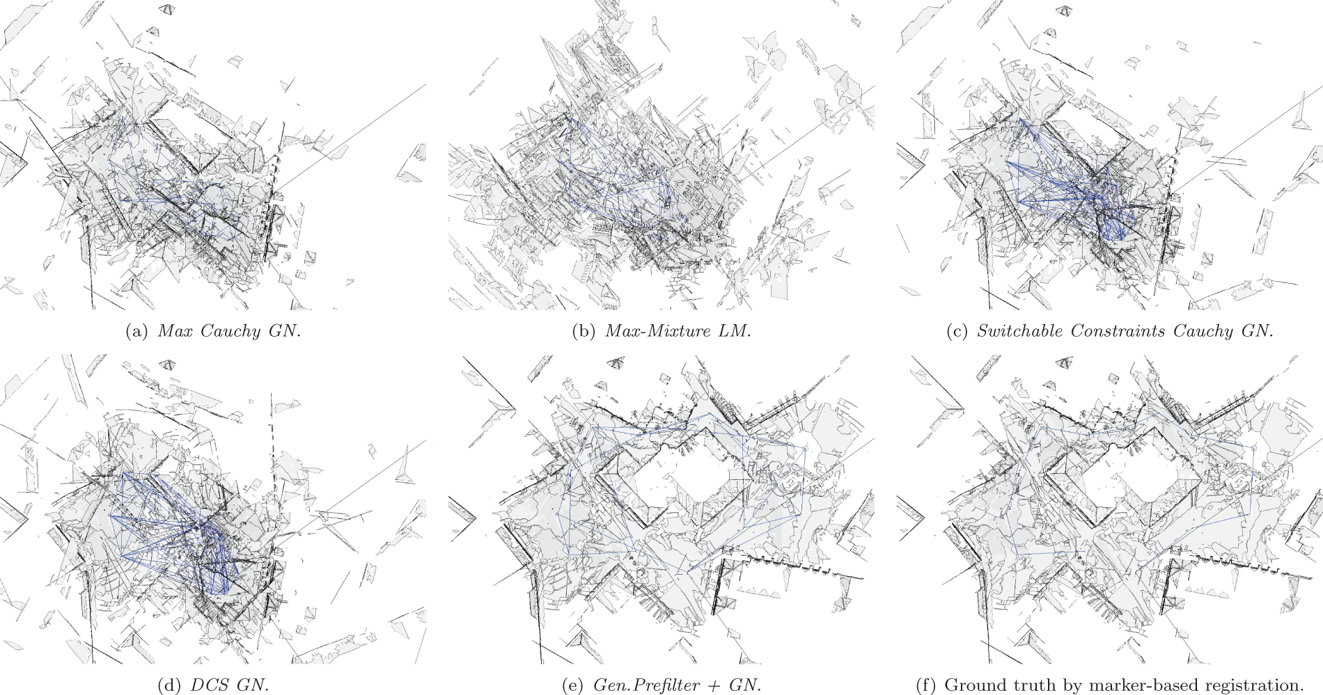
Orthographic view of the planar maps generated from the exhaustively matched Bremen City center dataset after optimization.

Fig. 13.

Perspective views of the planar maps generated by different SLAM methods with multimodal plane-matching and hyperedges from exhaustive loop-closing.

Switchable Constraints GN diverged far away from the ground truth, too far to visualize. With the Cauchy kernel, it converges to a similar local optimum as the Max Cauchy GN method. The result of Max-Mixture LM, while having a lower total rotation error, seems to be very off in terms of roll and pitch, showing building faces in the top-down orthographic view in Figure 12. The DCS GN method performs slightly better than Max Cauchy GN.

Again, much like in the synthetic dataset discussed in Section 5, the main reason for the failure of these methods is the initial guess. All methods were initialized with a breadth-first traversal of the graph using the most likely component, which is the locally best decision. Only Generalized Prefilter is designed to approximately pick the globally best component before the continuous optimization starts, all other methods converge to a local optimum. Once again, this shows the significant reliance of any optimization method on the initial guess.

Clearly, the Generalized Prefilter+GN method outperforms all others, both in the quality of the optimization result and efficiency. Note that the mean square errors SSE in the table are in mm², so the final SSE_xyz of 3.545 × 10⁴ corresponds to a mean distance of 0.18 m to each ground truth vertex pose. The next best result with 64.92 m is obtained by the DCS GN method.

Figures 12 and 13 show the 3D maps computed by the different methods. The changes in graph topology induced by the Generalized Prefilter method after rejecting inconsistent MoG and hyperedge components is especially visible in Figure 12 showing the map from the top with an orthographic projection.

8. Underwater visual SLAM on the Ligurian Sea dataset

This experiment again serves two main purposes. Firstly, it is also used for comparison to other approaches to robust SLAM within a different application domain, namely 2D visual SLAM. Secondly, it illustrates two general strategies to use Generalized Graph SLAM, namely the combination of multiple motion estimates in multimodal edges (Section 6.1.2) and lenient place recognition leading to hyperedges (Section 6.2.2). We consider each of the two underlying strategies on their own to be of high interest for mapping applications, independent of the specific implementations for complementary motion estimates and for place recognition that are used here.

The dataset used in this experiment was collected by the Romeo Remotely Operated Vehicle (ROV) of the Italian National Research Council (CNR) (see Figure 14) in the Summer of 2005 in the Ligurian Sea near Portofino, Italy (Caccia, 2006). The trial took 44 minutes and 15 seconds which corresponds to 13,275 processed images of 360X272 pixels at a 5 Hz rate and an area of approximately 23 m² at a depth around 20 m. The Romeo ROV navigated through waypoints along a two dimensional grid, also known as a lawn mowing pattern, in auto-altitude mode and at constant heading. Without diving and surfacing, as well as some setup time, the total number of useful images is 12,101. For more details about the setup refer to Caccia (2006).

Fig. 14.

The Romeo ROV used in the experiments. The image on the right side shows the monocular camera assembly.

Two complementary registration methods were used, a RANSAC-based method with an affine transformation model using SURF (Bay et al., 2008) features, and a spectral registration method called iFMI (Buelow et al., 2009; Pfingsthorn et al., 2010). Due to the uneven ground and the resulting parallax, the purely 2D affine model as used in both methods will calculate incorrect rotation. Correcting this registration artifact is only possible by more sophisticated methods or by sensing the heading directly with a compass. Since the data was recorded in constant heading mode, the rotation estimate for each registration result was set to zero, though the covariance values were not changed. This still leaves significant rotational error to be corrected during optimization. Both complementary registration methods produce a relative pose estimate between the two processed images including a covariance matrix. The quality metric required for the method sketched in Section 6.1.2 was computed using the percentage of detected inliers for RANSAC and the PNR metric for iFMI described in Pfingsthorn et al. (2010). Both methods were assigned equal weights, while the covariances scales ω were 1200 for RANSAC and 1 for iFMI. The scales were assigned empirically and their large difference stems from the vastly different methods used to assign covariances. In practice, since only inliers were used to compute the covariance of the RANSAC result, it severely underestimated the covariance, which is reflected in the large scale factor. The translation threshold ${\mathcal{T}}_{\min }$ was set to 1.5 pixels while the rotation threshold ${\mathcal{R}}_{\min }$ was not applied due to the correction described above.

The minimum place recognition quality ${\mathcal{Q}}_{\min }$ from FABMAP was set to 0.00025, significantly lower than the usual 0.99. Rather high, method-specific, maximum quality thresholds ${\mathcal{Q}}_{\max }$ , i.e. inlier percentage and PNR, as well as the requirement that the combined registration result must be unimodal were used to allow single loop registrations to become simple edges instead of components in the hyperedge. The Null hypothesis weight π₀ was set to 0 if both complementary registration methods agreed and were fused for all loop hypotheses, and 0.1 otherwise. This resulted in a pose graph which in a sense contains the set of edges a traditional conservative frontend would generate as a subset.

All 12,101 images were used to generate the maps in Figure 15. Thus, all resulting pose graphs also had 12,101 vertices. All sequential pairs were registered successfully, resulting in 12,100 sequential edges, 20 of which were multimodal. A total of 11,600 loop edges were constructed from hypotheses generated by the OpenFABMAP implementation (Glover et al., 2012) and processed into hyperedges as described in Section 6.2.2. Of these, 280 are hyperedges, and the rest are simple or multimodal. A more detailed breakdown by number of components is shown in Table 9. This results in a total graph complexity of 591.304, which is extremely high.

Fig. 15.

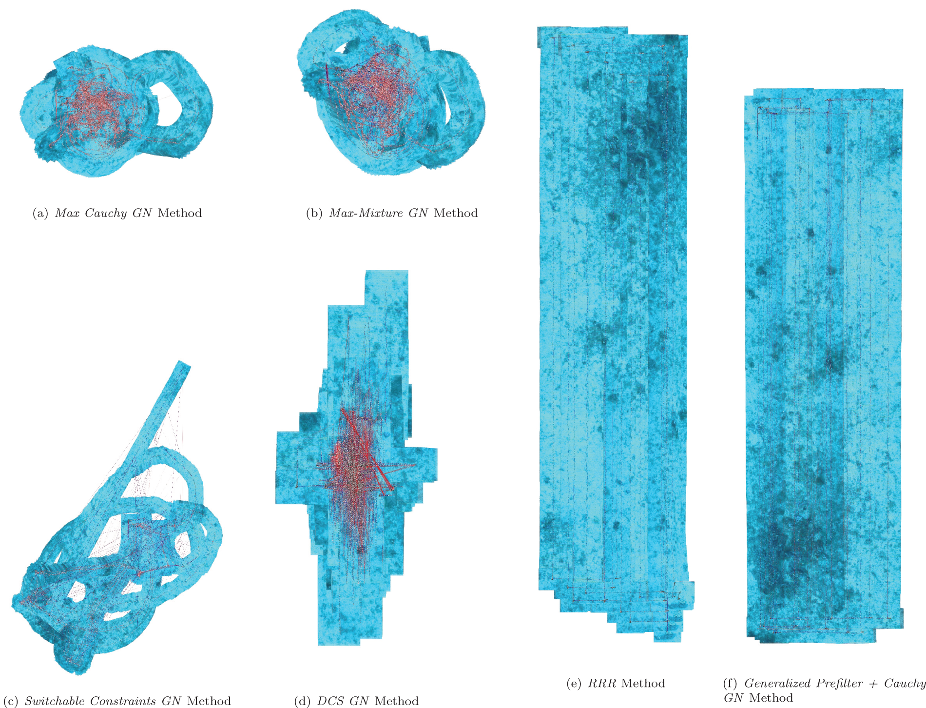
Maps generated by different optimization methods from the CNR Romeo dataset.

Table 9.

Distribution of the number of components on edge constraints. The largest loop hyperedge has 27 components. One hypercomponent signifies an edge with a single hypercomponent and without a Null hypothesis. All edges with two or more hypercomponents usually have a Null hypothesis.

Constraint Type	1	2	3	4	5	6	7+
Sequential Constraints
- Mixture components	12080	20
- Hypercomponents	12100
Loop Constraints
- Mixture components	11874	178	16
- Hypercomponents	11320	185	45	13	4	6	27

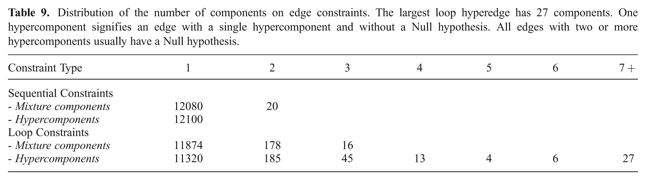
Figure 15 shows maps generated by all six evaluated methods. The parameters for these methods are the same as used in the evaluation with the synthetic data (Section 5). Note also the same suffixes denoting the exact optimization algorithm and robust kernel used in g²o. The results further support the outcomes from the systematic analysis with the synthetic data. The Max Cauchy GN method, which corresponds to the traditional unimodal case, naturally diverges significantly, even though a robust kernel is used. Note that the Max Cauchy GN method uses the locally best generated mode per edge, i.e. the highest weighted one, and thus uses the most certain registration result in case the two methods disagreed, not always the fused result. Similarly, the highest weighted mode is also selected out of all mixtures in any hypercomponent of a hyperedge.

Both the Max-Mixture GN and DCS GN methods converge to a similarly broken and collapsed result as the Max Cauchy GN method. DCS GN seems to recover small linear segments of the original trajectory, while Switchable Constraints GN is able to recover much longer segments. However, both methods do not succeed to correctly solving all ambiguities in the data. Again, this is a problem with the initial guess, which was seemingly too far away from the basin of convergence of these methods.

Out of all methods other than Generalized Prefilter+Cauchy GN, RRR achieves the best result. In contrast to the results of the systematic experiments above, RRR maintains connectivity, but falsely rejects all loop closures, resulting in a large drift along the trajectory. This is evident in the visible seams of the final photo map in Figure 15e. Generalized Prefilter+Cauchy GN achieves a consistent map by correctly solving local and global ambiguities simultaneously.

Table 10 shows the runtimes of the methods. Note that the fastest method across the board is Generalized Prefilter+Cauchy GN. The reported time includes all computations for both stages. However, the differences to the Max Cauchy GN, Switchable Constraints GN and DCS GN methods do not seem significant. The Max-Mixture GN method takes twice as long as Generalized Prefilter+Cauchy GN. More interestingly, the RRR method, which performed closest to Generalized Prefilter+Cauchy GN, takes three orders of magnitude longer.

Table 10.

Runtimes of the different optimization methods in seconds. Note the significantly larger runtime of the RRR method. Times are recorded on a Intel Core i7-3770, 3.40 GHz, with 16 GB RAM.

Method	Runtime (s)
Max Cauchy GN	8.52
Max-Mixture GN	15.41
Switchable Constraints GN	10.28
DCS GN	9.59
RRR	6450.6
Generalized Prefilter + Cauchy GN	8.26

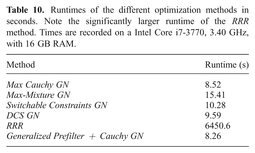
9. Conclusions

In this article, the Generalized Graph SLAM framework was presented, and a formal description of how to use hyperedges to encode uncertain loop closures was introduced. This tool for the representation of global ambiguities complements multimodal edges for local ambiguities. The representations used in current state-of-the-art methods in robust Graph-based SLAM were shown to be special cases of this Generalized Graph SLAM formalization.

Furthermore, a method to deal with multimodal hypergraphs in a unified coherent way was presented. This Generalized Prefilter method is introduced as an intermediate stage between the classical SLAM frontend and backend to remove both local and global ambiguities through a discrete optimization process. The method searches a combinatorial tree of component choices and resulting vertex poses formed by a spanning tree traversal of the multimodal hypergraph with beam search. Each component of a traversed ambiguous edge, either a multimodal MoG edge, a hyperedge, or a multimodal hyperedge, gives rise to a new subtree in this combinatorial search tree. Then, the best leaf of the search tree is selected and used to infer the chosen components during the traversal as well as to choose components of ambiguous edges that were not traversed. Finally, a disambiguated unimodal graph is generated using only the chosen components per ambiguous edge as well as initial estimates for the vertex poses.

The Generalized Graph SLAM framework is validated with experiments on synthetic graphs and as well as with real world datasets. The experiments showed that Generalized Graph SLAM with the Generalized Prefilter method is both significantly more robust and less computationally demanding than current state-of-the-art approaches with which it is intensively compared. Experiments with the standard Sphere2500 dataset showed that the final performance of Generalized Graph SLAM also depends on the subsequent robust continuous optimization in the backend, and the combination of Generalized Prefilter with a state-of-the-art robust backend (such as Dynamic Covariance Scaling) can be significantly more robust than the robust backend alone as soon as even a single MoG constraint exists.

Furthermore, the experiments with real world data also illustrate general strategies to build a SLAM graph with Generalized Graph SLAM. The 3D SLAM experiments with the Bremen City dataset showed how a registration method that generates a ranked list can be used to produce multimodal edges. The Generalized Graph SLAM framework simply allows the incorporation of multiple registration results as mutually exclusive choices if the ranking is not distinctive enough. In addition, the generation of hyperedges by exhaustive loop closures used in this experiment illustrated the robustness against false positives, which can be used for simple loop closure strategies.

The 2D visual SLAM experiments with the Ligurian Sea dataset illustrated two even more important use cases that are of general interest. Firstly, it showed how two separate motion estimates can complement each other as potentially mutually exclusive choices, instead of just fusing them which leads to less robust results. This is illustrated with two different registration methods in this experiment, but the same principle is also applicable to the combination of a single registration method with odometry. Secondly, it is shown how Generalized Graph SLAM can profit from lenient place recognition by incorporating ambiguities through trading off a high amount of correct loop closures with the existence of some or many false positives. This is done with the popular FabMAP method where we show that false positives in place recognition can only be avoided in the Ligurian Sea dataset at the cost of strict parameter settings that also lead to only very few loops.

Data

The base datasets as well as scripts to generate specific datasets used in experiments are available on github: https://github.com/maxpfingsthorn/OutlierGenerator .