So You’ve Got a High AUC,Now What? An Overview of Important Considerations when Bringing Machine-Learning Models from Computer to Bedside

Abstract

Machine-learning (ML) models have the potential to transform health care by enabling more personalized and data-driven clinical decision making. However, their successful implementation in clinical practice requires careful consideration of factors beyond predictive accuracy. We provide an overview of essential considerations for developing clinically applicable ML models, including methods for assessing and improving calibration, selecting appropriate decision thresholds, enhancing model explainability, identifying and mitigating bias, as well as methods for robust validation. We also discuss strategies for improving accessibility to ML models and performing real-world testing.

Highlights

• This tutorial provides clinicians with a comprehensive guide to implementing machine-learning classification models in clinical practice.

• Key areas covered include model calibration, threshold selection, explainability, bias mitigation, validation, and real-world testing, all of which are essential for the clinical deployment of machine-learning models.

• Following these guidance can help clinicians bridge the gap between machine-learning model development and real-world application and enhance patient care outcomes.

The application of machine learning (ML) has gained prominence in health care by offering sophisticated methods for identifying complex patterns within large datasets that traditional statistical approaches may otherwise overlook.^1,2 However, despite their impressive analytical capabilities, many ML models described in the academic literature remain confined to research settings and fail to progress toward widespread clinical adoption. ³ Similar to the bench-to-bedside journey in translational wet lab research, ML research teams must focus on the “computer-to-bedside” pathway to translate their in silico findings to practical patient care.

This article presents an overview of key considerations for designing clinically relevant ML models, including calibration, threshold selection, explainability, bias mitigation, and validation. These considerations align closely with principles outlined in authoritative guidelines for clinical model development, such as TRIPOD+AI. ⁴ In addition, we discuss strategies for successfully integrating these models into clinical workflows and approaches for evaluating their performance in the real world. Although the concepts presented are broadly applicable, we focus specifically on binary classification models that are widely used to assign discrete risk categories or outcomes in clinical settings.

Is Your Model Well-Calibrated?

When evaluating the performance of ML classification models, many published studies rely on familiar metrics such as accuracy, specificity, sensitivity, and the area under the curve of the receiver-operating characteristics curve (AUC-ROC). ⁵ These metrics are appealing because researchers commonly use them to evaluate traditional diagnostic tests that provide binary results (i.e., either positive or negative), ⁶ such as pregnancy or rapid COVID-19 antigen tests. However, ML models operate differently; rather than providing simple binary outcomes, they estimate the probability or risk of an outcome occurring. Most ML modeling packages then convert these continuous probability estimates into binary labels using a threshold, typically set at 50% by default. ⁷

While simple binary classifications may be sufficient in specific scenarios (e.g., in urgent care situations requiring rapid triaging), it is crucial to also provide the continuous probability estimates alongside binary labels, especially in patients with borderline risk probabilities. For instance, if a well-calibrated model predicts an outcome probability of 49% for one patient and 51% for another, using a 50% threshold would label the first patient as “low risk” and the second as “high risk,” despite their nearly identical outcome risk and similar clinical care needs. This issue is long-standing and not unique to ML models; similar challenges arise with thresholds in commonly used clinical tests such as prostate-specific antigen or HbA1c, for which patients just above and below the normal cutoff level have very similar clinical profiles. Evidently, in both clinical lab tests and when using ML models, providing continuous probability or quantitative values can offer clinicians more nuanced insights and facilitate better-informed medical decisions.

The extent to which a model can accurately predict probabilities is known as calibration. A well-calibrated model ensures its predicted probabilities closely match actual observed risks. For instance, if a model predicts an outcome probability of 20% for a patient group, we would expect approximately 20% of these patients to experience the outcome in practice. ⁷ Calibration is quantitatively assessed using metrics such as log loss (also known as cross-entropy loss) and the Brier score, ⁸ both of which measure the difference between predicted probabilities and observed outcomes. Lower scores indicate smaller differences, thus reflecting better calibration. Calibration can also be visually evaluated through calibration curves, ⁷ which plot predicted probabilities against observed probabilities in the dataset (Figure 1).

Figure 1

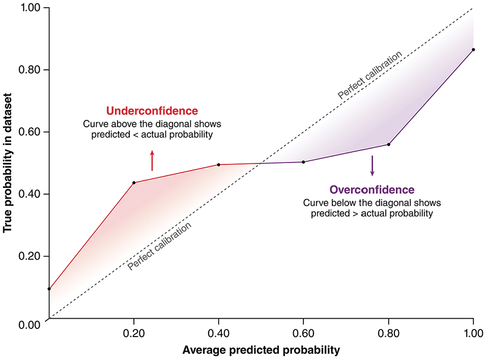
An example of calibration curves. Calibration curves illustrate the relationship between probabilities predicted by machine-learning models and the true probabilities from the training/testing dataset. The dotted diagonal line represents perfect calibration. The red section of the curve represents an underconfident model that underestimates outcome probabilities, and the purple section of the curve represents an overconfident model that overestimates outcome probabilities. As shown in this example, real calibration curves may contain a mix of segments where the model is underconfident, segments where the model is well-calibrated, and segments where the model is overconfident.

To achieve good calibration, clinical ML models should be tuned and selected based on calibration-specific metrics, such as log loss, instead of traditional performance metrics like AUC-ROC. It is important to note that calibration can be significantly disrupted by resampling techniques, such as oversampling the minority class or undersampling the majority class. Resampling aims to balance outcome classes in imbalanced datasets (e.g., datasets from studies involving rare events, in which most patients do not have the outcome); however, altering the outcome distribution inherently distorts the model’s probability estimates. ⁹ In general, resampling is unnecessary if a model is already well-calibrated and paired with a thoughtfully chosen threshold (see the following section). If resampling is essential, an additional posttraining calibration step—such as Platt scaling, ¹⁰ isotonic regression, ¹¹ or spline-based calibration ¹² —should be employed to realign the model’s probabilities with real-world risk probabilities.

Did You Select the Right Decision Threshold?

After ensuring that an ML model is well-calibrated, the next important step is selecting an appropriate decision threshold. As previously discussed, most ML modeling packages set a default threshold at 50%, which assumes an equal probability distribution between outcome classes (i.e., a 50/50 distribution). Unfortunately, clinical datasets frequently exhibit imbalanced outcome distributions, making this default assumption unsuitable. When predicting rare outcomes, a well-calibrated model often generates lower probability estimates for positive cases since the actual risks are low. Therefore, a 50% threshold could underestimate the number of positive cases. Conversely, if the outcome is very common, this default threshold might overestimate the number of positive cases, resulting in excessive false positives.

Several statistical methods are available to help identify a suitable threshold for imbalanced datasets. A commonly used method involves selecting a threshold that maximizes Youden’s Index in the training set or during cross-validation. ¹³ Youden’s Index is calculated as

$$Youde{n}^{\prime }sIndex=Sensitivity+Specificity-1$$

This metric determines a threshold that balances sensitivity (correct identification of patients with the outcome) and specificity (correct identification of those without the outcome).

However, using this “balanced” threshold relies on the additional assumption that false-positive and false-negative results have equal clinical consequences. Since clinical ML models do not exist in a vacuum, this assumption rarely holds true. It is thus essential to consider the practical implications of using the model in real-world patient care. For example, in scenarios such as cancer screening for an aggressive malignancy—where missing a diagnosis could significantly delay critical interventions—a lower threshold would be required to maximize sensitivity, despite an increase in false positives. Conversely, in contexts where false positives carry significant costs (e.g., prescribing medications with substantial side effects), a higher threshold that prioritizes specificity would be more appropriate. ¹⁴ Therefore, although a balanced threshold identified using Youden’s Index or similar metrics provides a useful starting point, it should mainly serve as a baseline for further threshold adjustments tailored to specific clinical scenarios (Figure 2) or as a benchmark for comparative model evaluations, rather than being directly adopted for clinical practice.

Figure 2

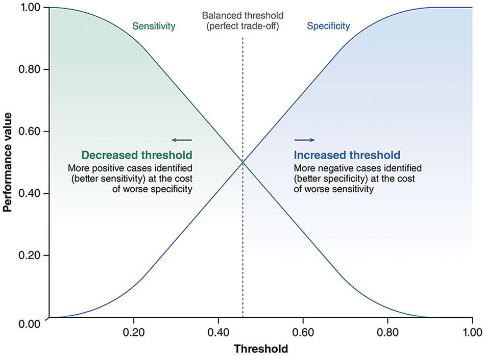
An example plot showing the typical change in sensitivity and specificity across different threshold values for a machine-learning model. As shown in this example, the threshold selected using metrics such as Youden’s Index (represented by the dotted line) provides a balanced tradeoff between model sensitivity and specificity; however, this is not always ideal in clinical practice. Depending on the clinical context, the threshold can be decreased to prioritize sensitivity or increased to prioritize specificity.

Do You Know How Your Model Is Making Its Predictions?

One of the major barriers to clinical adoption of ML models is the difficulty in understanding how these models reach their predictions—a concept known as explainability. ¹⁵ Simpler algorithms, such as logistic regression or decision trees, can provide straightforward explanations by design (Figure 3).^16,17 In contrast, more complex algorithms—such as neural networks and ensemble methods like random forest—are often described as “black boxes” because their decision-making processes are opaque. ¹⁸ Without clear explainability, ML research teams might struggle to identify biases or errors within these models, and clinicians may hesitate to trust the model predictions if they cannot verify whether the model’s logic aligns with established medical knowledge and clinical evidence.^19–21

Figure 3

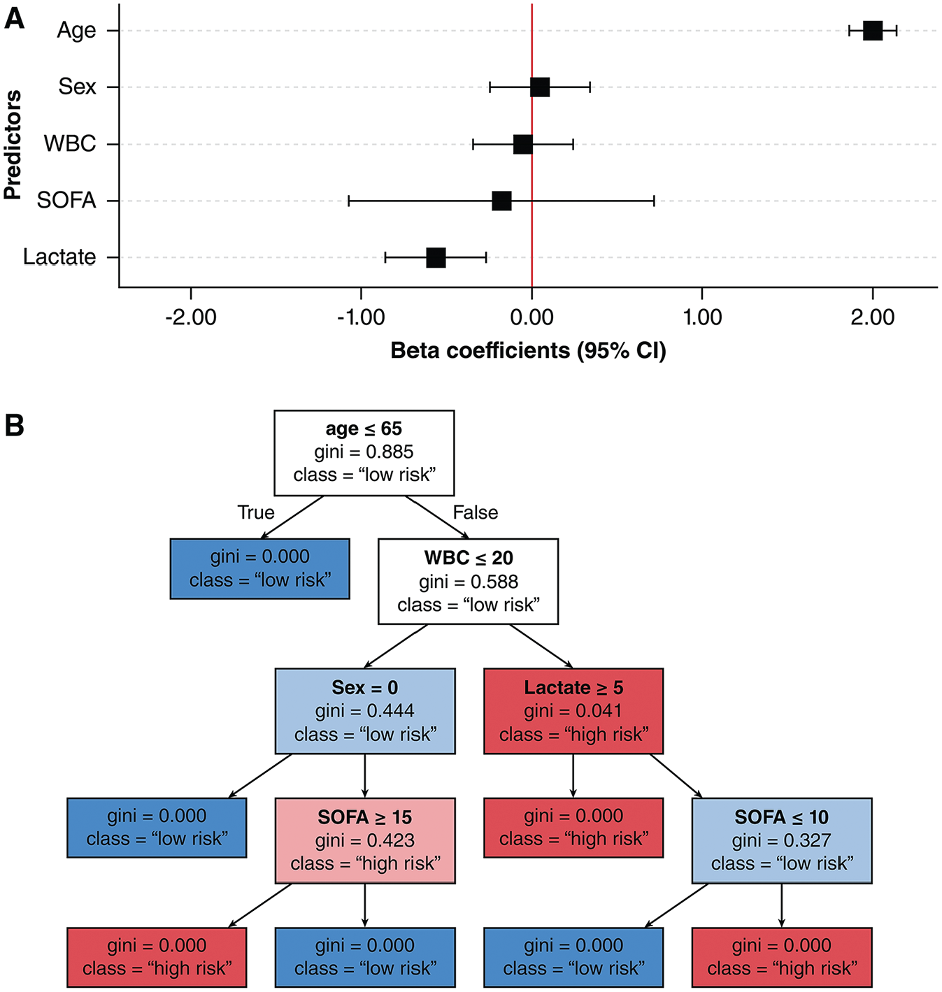
Examples of explainability plots for simpler, transparent machine-learning models. (A) An example of a coefficient forest plot for a logistic regression model, which shows the magnitude, direction, and uncertainty of predictors’β coefficient on outcome predictions. (B) An example of tree visualization for a decision tree model, which shows the predictors and cutoff values used to facilitate outcome classifications.

A well-known example illustrating the critical importance of explainability involves computer vision models trained to detect skin cancer. Some models unintentionally learned to associate irrelevant markers—such as pen markings and rulers often present in dermatologic images—with malignant lesions, rather than focusing on clinically meaningful features such as lesion color or border irregularities.^22–25 Without explainability methods, such misleading associations can result in models that appear effective on paper yet remain clinically untrustworthy and impractical.

Explainability methods can be broadly categorized as global or local. Global explainability addresses how a model generally makes predictions across the entire dataset. One widely used global explainability method is permutation importance (Figure 4A). It works by first calculating baseline model performance (e.g., using AUC-ROC) on the training or validation dataset (Figure 5A). Next, values of a single predictor are randomly shuffled among patients, which effectively breaks its relationship with the outcome. This shuffling process is called perturbation (Figure 5B). The model’s performance is then reassessed with the shuffled data; a significant decrease in performance indicates that the predictor was influential to the model (Figure 5C). ²⁶ Permutation importance is notably limited by its assumption of predictor independence. With highly correlated variables (e.g., body weight and body mass index), shuffling one may minimally affect performance because the model can rely on correlated predictors to maintain predictive accuracy. This can result in underestimations of true importance in these correlated predictors. ²⁷

Figure 4

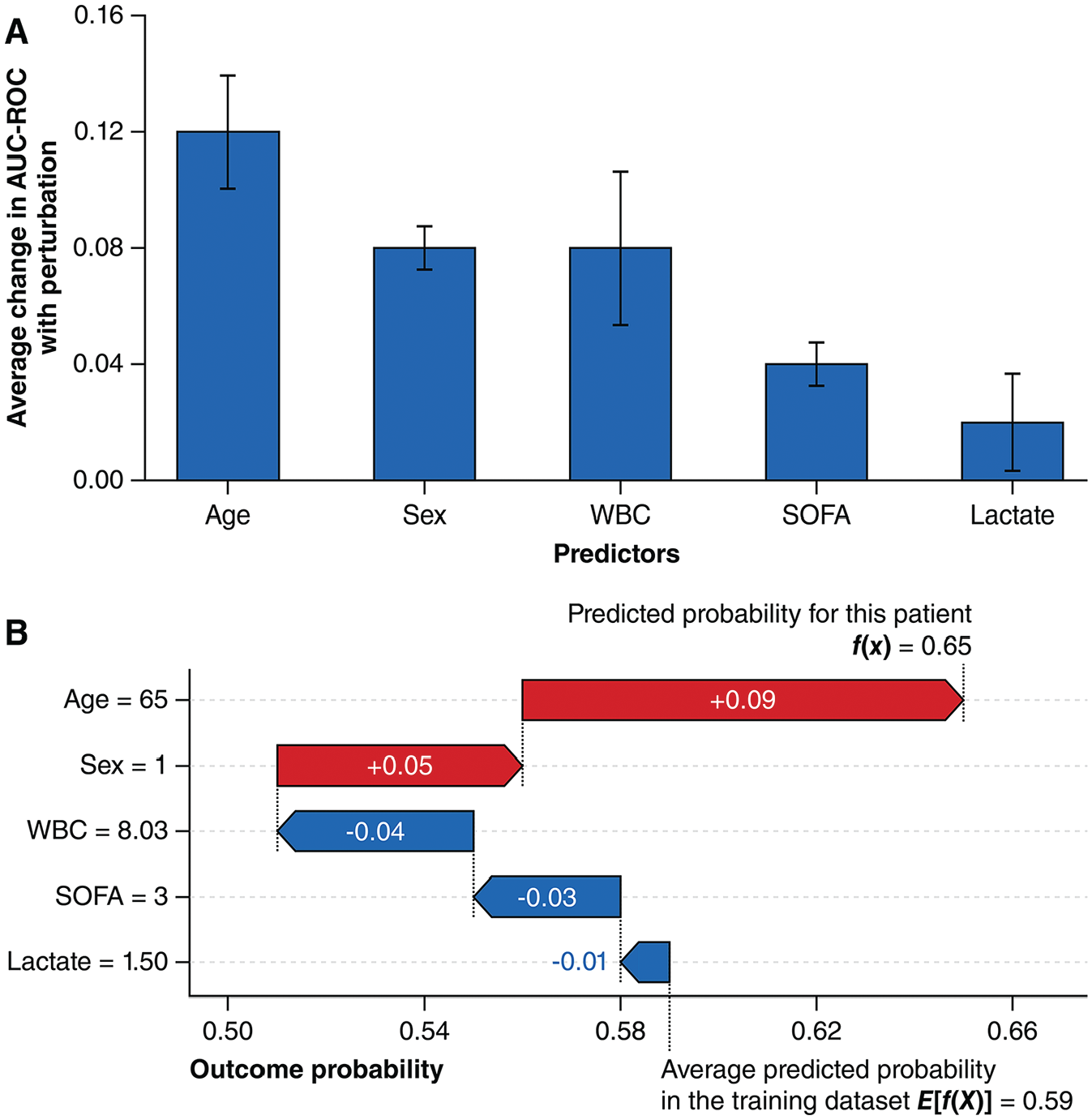
Examples of explainability plots for complex, “black-box” machine-learning models. (A) An example of a permutation importance plot. Predictor perturbations are usually repeated many times during permutation importance assessments, and the performance impacts are averaged. The resultant variance is represented by the error bars in the plot. (B) An example of a SHapley Additive exPlanations (SHAP) waterfall plot illustrating the local explainability for a single prediction. SHAP waterfall plots are read from the bottom to the top. Starting at the average predicted probability of all patients in the training dataset, different predictors either increase (colored red) or decrease (colored blue) the predicted probability to reach the final predicted probability.

Figure 5

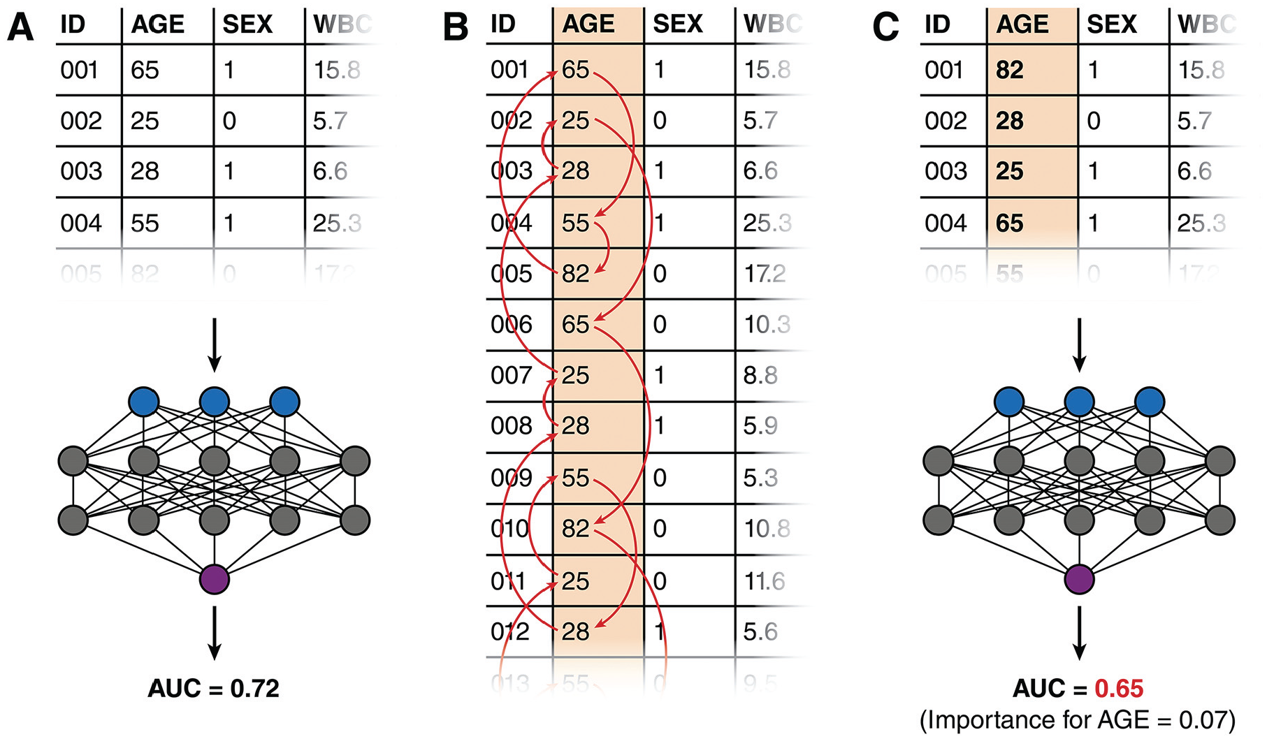
Steps for assessing the permutation importance of a machine-learning model. (A) A baseline performance metric is first obtained by running the training dataset or a validation dataset through the model. (B) Values from one predictor column are randomly shuffled among the patients. (C) A new performance metric is obtained by re-running the dataset (now with the shuffled predictor) through the model again. The change in performance metric represents the importance of the shuffled predictor.

Local explainability methods, such as SHapley Additive exPlanations (SHAP), ²⁸ explain how models make predictions for individual patients (Figure 4B). SHAP quantifies each predictor’s contribution to a predicted probability through “Shapley” values, ²⁹ which originate from cooperative game theory—a mathematical framework originally developed to fairly distribute contributions among collaborating workers.^30,31 A popular, model-agnostic SHAP method is “permutation” SHAP, which employs a similar approach to permutation importance.^28,32 Instead of shuffling predictor columns (which is not possible for a single patient), predictor values are replaced by randomly drawn values from the model’s training dataset. The resulting changes in the predicted probability, rather than performance metrics, are measured. Unlike permutation importance, Permutation SHAP perturbs combinations of predictors rather than one predictor at a time and calculates the average change in probability attributed to each predictor across these perturbations. This approach allows permutation SHAP to effectively account for predictor interactions and correlations.

Although SHAP is primarily used to explain individual predictions, it can also be aggregated across multiple patients to provide global explainability similar to permutation importance without assuming independence between predictors. Permutation importance is conceptually simpler and less computationally expensive, but aggregated SHAP may be preferable for providing global explainability in datasets with highly collinear predictors.

In image-based classification models, techniques such as gradient-weighted class activation mapping (Grad-CAM) ³³ can provide local visual explanations by highlighting areas of the image that were most influential in the model’s decision-making process (Figure 6). Such visual explanations can help clinicians verify whether models focus on clinically meaningful features, such as a lesion, rather than irrelevant artifacts. ³⁴

Figure 6

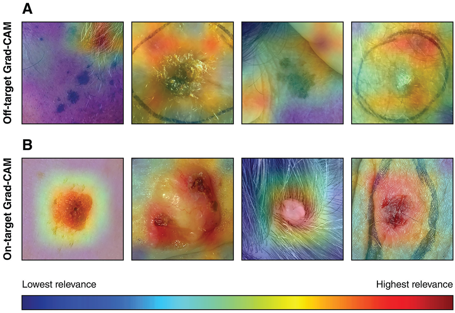
Examples of gradient-weighted class activation mapping (Grad-CAM) heatmaps for an image-based classification model for identifying skin cancer. Areas colored in red are considered highly relevant for the model during classification. (A) Examples of off-target Grad-CAM heatmaps. The model incorrectly focuses on elements such hair, skin folds, or marker lines rather than the lesion. (B) Examples of on-target Grad-CAM heatmaps where the model correctly focuses on the skin lesion. The skin lesion images shown originate from the PAD-UFES-20 skin lesion dataset, ³⁵ and they were made available under a CC BY 4.0 license (https://creativecommons.org/licenses/by/4.0/).

Is Your Model Free from Biases?

Apart from helping to identify erroneous predictions and foster clinician trust, explainability can also reveal biases in ML models. Biases in ML models typically originate from their training data, which often reflect historical and systemic health care inequities.^36,37 For instance, ML algorithms used by US health care insurance companies have previously been shown to allocate fewer resources to Black versus White patients. This disparity was not due to genuine differences in health care needs but because the models’ training data showed historically lower health care expenditures for Black patients—often a consequence of unequal access to health care services. ³⁸ As a result, Black patients, who in fact tend to have higher disease burdens, received even fewer resources due to this algorithmic bias. Similarly, many dermatology training datasets predominantly contain images of lighter skin phototypes, ³⁹ which reflects a historical lack of dermatological care access among people of color. ⁴⁰ Consequently, these models may perform poorly on patients with darker skin phototypes, potentially leading to misdiagnosis and suboptimal care. ⁴¹

Explainability methods can identify biases by revealing whether demographic factors such as race or gender disproportionately influence predictions despite a lack of clear medical justification. In addition, subgroup analyses can further quantify potential disparities in model performance across demographic groups. Two frequently employed fairness criteria in subgroup analyses include equal odds and equal opportunity. Equal odds ensure similar true-positive and false-positive rates across demographic groups, whereas equal opportunity specifically ensures similar true-positive rates across groups. ⁴² Similar to threshold selection, the choice between these 2 metrics is driven by clinical context and the intended use cases of the model.

To effectively mitigate biases during model development, it is essential for ML research teams to actively identify demographic groups that have been historically under- or misrepresented in health care datasets. Engaging stakeholders from these underrepresented communities can offer valuable insights into potential sources of bias. If certain demographic groups are underrepresented, techniques such as resampling with synthetic data or configuring the model to place more weight on underrepresented samples can help balance the dataset. During training, models can be explicitly optimized for fairness metrics alongside traditional metrics such as log loss. Posttraining, setting different decision thresholds or recalibrating for different demographic groups can also help achieve fairness objectives.

A commonly used but flawed bias mitigation strategy is excluding sensitive variables such as race or gender entirely from modeling, a practice known as “fairness through unawareness.” Removing these variables does not eliminate bias, as correlated features (e.g., genetic markers or geographic location) may implicitly reintroduce demographic information and perpetuate bias. ⁴³ Instead, retaining these sensitive variables to allow for fairness evaluations and targeted adjustments, as discussed above, is the recommended approach.

When complete bias elimination is not feasible, transparency is critical. Clinicians who use the model should be informed about any known biases in the model’s training data, and the use of the model should be limited to populations adequately represented in the dataset. By prioritizing bias identification and mitigation, ML models can contribute to more equitable health care outcomes rather than perpetuating existing disparities during clinical decision making.

Is Your Model Properly Validated?

Before deploying an ML model in clinical practice, thorough validation is essential to detect “overfitting,” in which a model performs well on its training dataset but generalizes poorly to new datasets. ⁴⁴ Validation typically involves 2 stages: internal and external validation. Internal validation assesses the model’s performance on a held-out portion of the original dataset, commonly referred to as a “test set,” which was not involved in training. This type of validation provides initial performance metrics and helps identify any immediate issues related to overfitting. However, since the test set comes from the same source as the training data and thus shares similar characteristics, it may not fully capture how the model will perform in real-world settings. ⁴⁵

External validation is necessary to accurately evaluate the true generalizability of a model. It involves testing the model on an entirely independent dataset—ideally from different institutions, patient populations, and/or time periods compared to the training dataset. External validation is more effective in detecting overfitting and provides greater assurance that the model will perform reliably beyond its original context. ⁴⁵

While external validation is ideal, obtaining an independent validation dataset can be challenging and time-consuming. When external validation is not feasible, nested cross-validation offers an alternative approach. Nested cross-validation evaluates the generalizability of the entire model development process rather than an individual model. It involves repeatedly dividing the dataset into different training and testing subsets through a cross-validation approach (i.e., the “outer” cross-validation loop; Figure 7A). Within each training subset, the model is tuned and selected using an additional cross-validation step as normally done during model development (i.e., the “inner” cross-validation loop; Figure 7B). The model’s performance is then evaluated on the corresponding testing subsets, with results averaged across the subsets (Figure 7C–E). This approach can be considered as a form of repeated internal validation. Nested cross-validation maximizes the modeling pipeline’s exposure to unseen data and provides a robust estimate of both the pipeline’s generalizability and performance variability, particularly when data availability is limited. ⁴⁶

Figure 7

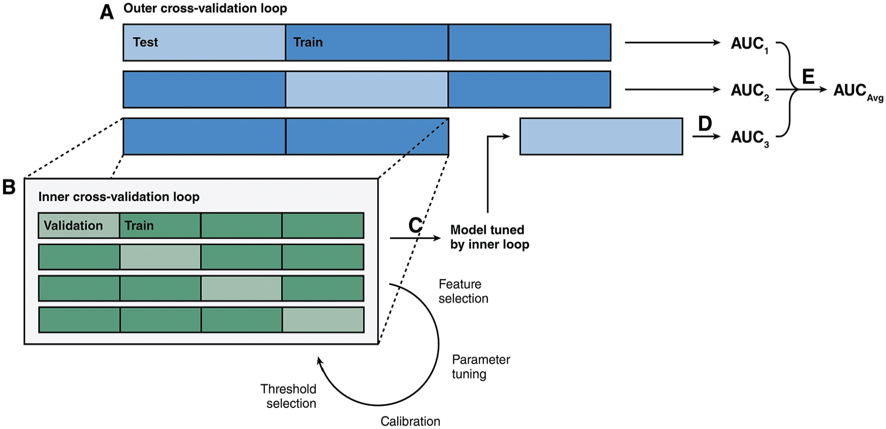
Illustration showing the structure of a nested cross-validation methodology. (A) First, the dataset is split into different training (colored dark blue) and testing (colored light blue) subsets through cross-validation. In this example, 3 outer folds were used. (B) Each training subset is further divided into different training (colored dark green) and validation (colored light green) subsets through cross-validation. In this example, 4 inner folds are used. The inner cross-validation loop facilitates typical model development steps such as feature selection, hyperparameter tuning, calibration, and threshold selection. (C) Once the optimal model configuration is selected by the inner cross-validation loop, the model is trained on the entire training subset. (D) The model is then tested on the corresponding testing subset to generate performance metrics. (E) The performance metrics from all outer cross-validation loop are averaged to produce the nested cross-validation metric.

How Will Clinicians Access Your Model?

When deploying ML models in clinical settings, it is important to consider how clinicians will practically interact with these tools. Most health care professionals are not experts in programming or statistical software; indeed, more than 20% of health care staff report experiencing anxiety when using information systems. ⁴⁷ Asking clinicians to download code from GitHub, run Python programs, or input patient data into statistical software such as R is likely a fruitless affair.

One effective solution is to develop web-based clinical risk calculators. An example of this approach is the American College of Surgeons Risk Calculator (https://riskcalculator.facs.org/), ⁴⁸ which is designed to predict short-term postoperative complications. Frameworks such as Shiny (https://www.shinyapps.io/), Streamlit (https://streamlit.io/), or Dash (https://dash.plotly.com/) can simplify the creation of these tools. For larger models requiring many predictors, direct integration into electronic health record (EHR) systems is often the best solution. Collaborating with system administrators or EHR developers can facilitate automated data entry, which reduces human errors and streamlines clinical decision making.

Building on the considerations discussed earlier, ML-based clinical risk calculators should provide both easily interpretable binary classifications based on clinically relevant thresholds as well as continuous probability estimates. They should also incorporate local explainability methods, such as SHAP, to visually illustrate which predictors contribute most significantly to the current prediction. Screening questions or demographic information from EHR systems can determine whether the patient is adequately represented by the training dataset or guide the application of demographic-specific models or thresholds to minimize bias.

Apart from these technical considerations, ML research teams must ensure that the calculator interfaces are accessible and intuitive. Usability testing involving clinician colleagues and other potential users can help identify confusing or unintuitive design elements. Clear, simple interface design is essential for ensuring the tool is user friendly and does not add unnecessary complexity to clinical workflows.

Given that these calculators use sensitive patient information, information security is another critical consideration. These tools should request only the minimum necessary information to generate predictions and avoid collecting irrelevant protected health information, such as patient names or medical record numbers. In addition, certain ML models and explainability techniques, such as k-nearest neighbors and SHAP, require access to the full training dataset at runtime,^28,49 which poses privacy risks if deployed on unsecured or public servers. These privacy risks can be mitigated by deploying models on secure institutional devices, using privacy-preserving model variants, ⁵⁰ or generating synthetic datasets that mimic the original dataset’s characteristics for deployment purposes. ⁵¹

Depending on the jurisdiction where the model will be used, there may be regulatory and institutional requirements that must be addressed before ML-based clinical risk calculators can be used in patient care. While proof-of-concept software developed for research purposes is often exempt from strict regulations, models intended for broader clinical or commercial use must comply with applicable legal standards. In the European Union, transparency and explainability of clinical ML models are mandated under the General Data Protection Regulation and the Artificial Intelligence Act.^52,53 In the United States, the Food and Drug Administration (FDA) classifies clinical ML tools as Software as a Medical Device (SaMD), which subjects them to rigorous safety, efficacy, and quality assurance standards similar to other medical devices. ⁵⁴ Certain ML-based tools deemed “high risk” for patients under the current FDA regulatory framework may even require an extensive premarket approval process involving detailed clinical validation as well as ongoing postmarket surveillance to ensure patient safety. ⁵⁵ The FDA, alongside other national regulatory bodies, provide guidelines such as the Good Machine Learning Practice for Medical Device Development, ⁵⁶ which ML research teams and developers should follow when designing clinical ML tools with the goal of obtaining regulatory approval.

From an institutional perspective, clinical risk calculators must incorporate auditing mechanisms to maintain accountability for medical decisions based on their predictions. For models integrated into EHR systems, input variables, model-generated predictions, and clinicians’ acceptance or rejection of model recommendations (along with justifications, if applicable) must be logged. When a clinician applies the tool to patients inadequately represented in training datasets, they must explicitly acknowledge the model’s limitations, and these acknowledgments must also be recorded. Institutions should retain these detailed audit trails to ensure regulatory compliance and for potential medicolegal purposes.

Do You Have Plans to Expand Your Model in the Future?

After the initial development of clinical ML models, they should be continuously updated with new patient datasets as they become available. These updates are beneficial because ML models generally improve in accuracy and generalizability when trained on larger and more diverse datasets.^57,58 In addition, the clinical characteristics of patient populations and the relationships between predictors and outcomes may change over time and cause a decline in model performance—a phenomenon known as “data drift.”^59,60 For example, a model initially developed based on a younger local population with few comorbidities might lose predictive accuracy as the population ages and develops more complex medical issues.

Despite the importance of ongoing updates, most algorithms cannot adapt to new data on the fly. ⁶¹ Efforts to develop ML systems capable of continuous learning often encounter challenges, such as “catastrophic forgetting,” where the introduction of new data leads to loss of previously acquired knowledge and subsequent performance degradation. ⁶² Consequently, incorporating new data into an existing model typically requires retraining and retuning the model from scratch. Given the resource-intensive nature of retraining, careful consideration must be given to determining when and how frequently to update the model. If the model relies on a continuously updated registry, establishing a regular update schedule may be necessary. Alternatively, updates could be triggered by the availability of a significant amount of new data, ensuring that the model remains current without unnecessary retraining.

Beyond periodic updates, ML research teams should consider strategies for scaling their initial institutional modeling efforts into multicenter collaborations. Expanding training datasets by partnering with other institutions has been shown to significantly enhance model generalizability. ⁶³ However, multicenter collaborations can be challenging due to varying regulatory and institutional policies regarding patient data sharing. One way to managing these challenges involves a “distributed ensemble” approach, in which local models are first independently trained at each participating institution and later combined into a global ensemble model using techniques such as “bagging,” in which multiple models collectively “vote” on a classification or average their probability estimates to generate a final prediction (Figure 8A). ⁶⁴ This approach allows institutions to maintain ownership over their data while contributing to a more robust and generalizable global model. In addition, data from new institutions can be easily incorporated as additional local models; existing local models do not need to be retrained.

Figure 8

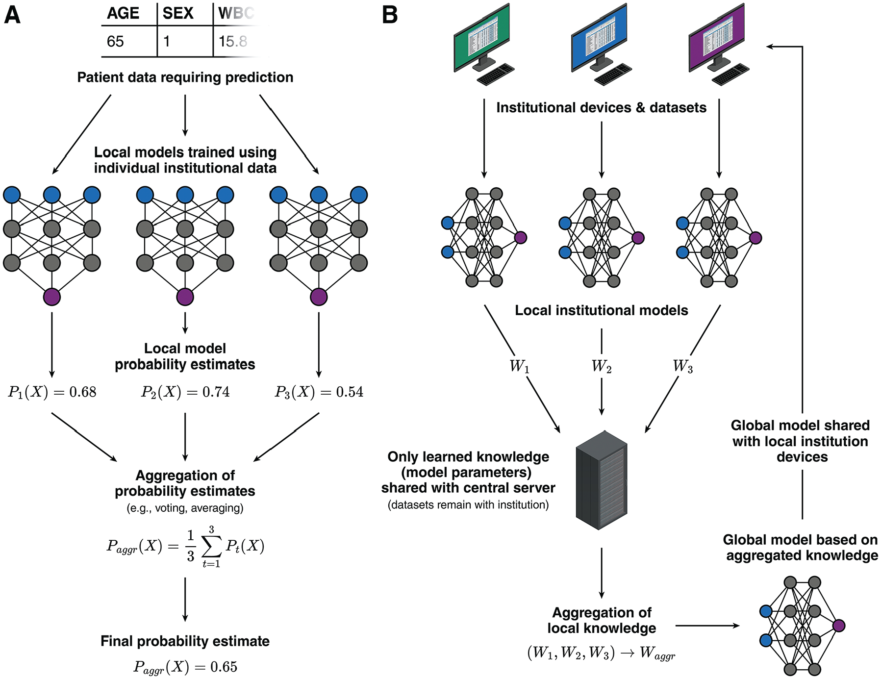
Illustration showing strategies for facilitating multicentered collaboration during machine-learning model development. (A) Schematic for a “distributed ensemble” approach, in which each institution trains a local model using their local datasets. When a prediction is needed, each local model generates a probability estimate based on the patient data, and these probability estimates are aggregated through methods such as voting or averaging to produce a final probability estimate. (B) Schematic for a federated learning approach. A central server coordinates the training of local models at each institution using their local datasets. The server periodically collects the model parameters (such as weights from neural networks, which carries learned knowledge) from each institution and aggregates them into a global model. This global model is then redistributed back to each institution for use or for improving the local model.

A more structured and advanced implementation of this collaborative approach is federated learning. Federated learning systematically coordinates the training of local institutional models through a central server. The central server periodically aggregates model parameters from local models, such as weights from neural networks, into a global model. The updated global model parameters, which carry the learned knowledge from all sites, are then shared with each participating institution (Figure 8B). ⁶⁵ This method enables automated training of multicentered neural networks while preserving patient privacy and complying with data protection regulations.

Does Using Your Model Actually Improve Patient Outcomes?

While well-performing ML models can theoretically improve patient outcomes, there may always be unforeseeable real-world challenges that limit their practical usefulness. For example, the cost associated with managing or renting server infrastructure needed for deploying large models might outweigh the economic benefits provided by ML-driven predictions. In addition, models may rely on predictors that are difficult to obtain in routine clinical practice. For instance, image-based models often involve complex preprocessing and segmentation steps that may be impractical for typical clinicians. Similarly, models may require laboratory tests that are commonly used in research but rarely ordered in regular practice. Models needing extensive data input may inadvertently delay care due to the time required to gather and input the necessary information. These practical considerations are challenging to fully assess through computational testing alone.

Therefore, ML models must demonstrate their real-world value through structured clinical studies, similar to how new medications undergo rigorous clinical trials after laboratory development. This process can begin with “shadow testing,” in which investigators enter patient data into the ML model as though it were being actively used for clinical decision making. During shadow testing, model predictions remain hidden from clinicians and are not used for patient care. This approach allows researchers to compare model predictions directly with patient outcomes to highlight performance gaps and identify scenarios in which model outputs conflict with established clinical practices. Shadow testing can also uncover usability issues, such as the practical availability of required predictors in everyday clinical settings.

Following shadow testing, observational feasibility studies can be conducted, in which a small group of clinicians voluntarily integrates the model into their clinical decision-making processes. These studies may use cohort or before–after study designs. This stage is critical for gathering further feedback about the model’s utility, clinician–model agreement, and preliminary assessments of patient benefit or harm. If the model demonstrates potential for improving outcomes without significant risks, it can subsequently advance to pilot and large-scale randomized controlled trials.

Randomized trials represent the gold standard for rigorously evaluating the clinical impact of ML models. Ideally, these trials would be multicentered to ensure the generalizability of trial findings. These trials can employ a cluster-trial design, in which randomization occurs at the health care provider level rather than individual patient level. In such trials, clinicians in the intervention group have access to the ML-based clinical tools, while those in the control group do not. Importantly, clinicians should retain autonomy to rely on their clinical judgment and not be compelled to implement the ML tool’s recommendations, to better reflect realistic clinical practice. This design enables holistic evaluation of the ML tool beyond predictive accuracy, including clinician trust/adoption and integration into—or potential disruption of—clinical workflows.

After successful randomized trials, longitudinal follow-up studies are necessary to monitor sustained performance and cost-effectiveness across diverse clinical environments. Continuous evaluation helps detect and address ongoing challenges, such as data drift, to ensure that clinical ML tools remain sustainable and beneficial in the long term.

Conclusion

ML models have the potential to revolutionize health care by moving away from a “one-size-fits-all” approach toward more personalized, patient-centered care. Although the development process for ML models typically emphasizes optimizing performance metrics, it is crucial to remember their ultimate goal: improving patient outcomes in clinical practice.

Developing a practical ML model requires ML research teams and developers to consider a wide range of factors beyond model accuracy alone. As outlined in model development guidelines such as TRIPOD+AI, ⁴ ML models must be properly calibrated, rigorously validated, free from biases, and easily accessible to health care professionals. In addition, successful integration of these models into clinical workflows demands careful attention to usability, regulatory compliance, ongoing need for updates and collaborative expansions, as well as real-world testing. By carefully addressing these challenges, clinicians, researchers, and developers can collectively bridge the gap between model development and clinical practice to fully leverage ML’s transformative potential for enhancing patient care.