Sage Journals: Discover world-class research

Abstract

Economic evaluations conducted alongside randomized controlled trials are a popular vehicle for generating high-quality evidence on the incremental cost-effectiveness of competing health care interventions. Typically, in these studies, resource use (and by extension, economic costs) and clinical (or preference-based health) outcomes data are collected prospectively for trial participants to estimate the joint distribution of incremental costs and incremental benefits associated with the intervention. In this article, we extend the generalized linear mixed-model framework to enable simultaneous modeling of multiple outcomes of mixed data types, such as those typically encountered in trial-based economic evaluations, taking into account correlation of outcomes due to repeated measurements on the same individual and other clustering effects. We provide new wrapper functions to estimate the models in Stata and R by maximum and restricted maximum quasi-likelihood and compare the performance of the new routines with alternative implementations across a range of statistical programming packages. Empirical applications using observed and simulated data from clinical trials suggest that the new methods produce broadly similar results as compared with Stata’s merlin and gsem commands and a Bayesian implementation in WinBUGS. We highlight that, although these empirical applications primarily focus on trial-based economic evaluations, the new methods presented can be generalized to other health economic investigations characterized by multivariate hierarchical data structures.

Keywords

cluster randomised controlled trials cost-effectiveness analysis economic evaluation alongside randomised controlled trials multicentre and multinational randomised controlled trials

Economic evaluations conducted alongside randomized controlled trials (RCTs) are a popular vehicle for generating high-quality evidence on the incremental cost-effectiveness of competing health interventions. Typically, in these studies, resource use (and by extension, economic costs) and clinical or preference-based health outcomes data are collected prospectively for trial participants to estimate the joint distribution of incremental costs and incremental benefits associated with the intervention, taking into account fixed and random sources of variation.^1,2 The term fixed and random source of variation, as used in this article, refers to the set of explanatory variable(s) whose effect on the response is either assumed to be constant (fixed source of variance) or to vary randomly (random source of variance) across different realizations of the explanatory variable.³ Both sources of variance are commonly encountered in cost-effectiveness data generated from clinical trials, the former because of differences in patient characteristics and the latter as a consequence of study design, such as decisions to randomly allocate patients in clusters rather than individually (as in cluster-randomized trials), to recruit across multiple locations (as in multicenter and multinational trials), or to measure outcomes at multiple time points during follow-up (repeated measures).

Joint modeling of treatment costs and benefits, in cost-effectiveness analyses based on data from clinical trials, is often motivated by a desire to properly characterize uncertainty around estimates of incremental cost-effectiveness and display results graphically as cost-effectiveness planes and cost-effectiveness acceptability curves. If the outcomes are sufficiently correlated, there may be additional benefit from being able to borrow information across outcomes and estimate variance components and standard errors around parameter values more efficiently than in separate univariate analyses.⁴ However, joint modeling of multiple outcomes is a complicated statistical task if the data are not normally distributed and the outcomes are of different data types, such that a single probability distribution cannot wholly characterize their joint distribution.^5,6 In such situations, the simplest and most straightforward approach is to model outcomes separately by assuming appropriate distributional forms for each data type but allow the underlying parameters to be correlated or related in some way. This approach requires flexible software for implementation, something that has not been readily available in general-purpose statistical programming packages, such as Stata and R, familiar to many analysts working on trial-based economic evaluations. As an example, the methodology for analyzing economic data from clinical trials of the type described above has received substantial attention in the literature: published methodological papers include bivariate regressions for economic evaluations based on multicenter and multinational clinical trials (see references 7–9 and the citations therein), cluster-randomized trials,^10–12 and methods for modeling hierarchical cost data,^13–15 including extensions to allow for modeling health care costs and cost-effectiveness in the presence of structural zeros.^14,15 In all but the most straightforward situations where it is reasonable to assume normality of outcomes,¹¹ implementation of the methods outlined in these articles requires modeling on the net benefit scale⁸ or familiarity with specialized Bayesian and multilevel modeling software packages, such as WinBUGS,¹⁶ JAGS,¹⁷ MLwiN,¹⁸ or the SAS GLIMMIX procedure.⁶ An alternative approach that can be implemented in most statistical packages is the bootstrap.^1,19 It has the advantage of avoiding parametric assumptions about the data; however, it is computationally intensive, especially for complex analytic and missing data problems, as it requires repeated resampling of the data many times to accurately approximate the empirical distribution of the parameters of interest.^1,19

Recently, 2 new functions have become available (Stata gsem²⁰ and merlin²¹ in both Stata and R) that allow increasingly complex analysis to be conducted, including modeling multiple outcomes of mixed data types and their extensions to longitudinal and time-to-event outcomes.^21,22 The new functions use more accurate numerical integration techniques such as the adaptive Gaussian-Hermite quadrature to approximate the model and estimate parameters by maximum likelihood. However, maximum likelihood is known to underestimate variance components in mixed-effects models as well as standard errors of parameter values more generally in small to moderate sample size applications (i.e., the data for the analysis is small in relation to the number of parameters to be estimated).^23,24 The bias in the maximum likelihood estimate of variance components can often be corrected by restricted maximum likelihood,^23,24 but this can be difficult to implement via methods that approximate the likelihood for the data numerically.

In this article, we extend the generalized linear mixed-model framework to enable simultaneous modeling of multiple outcomes of mixed data types based on pseudo or quasi-likelihood methods previously proposed by Breslow and Clayton,²⁵ Wolfinger and O’Connell,²⁶ and Lindstrom and Bates²⁷ for nonlinear mixed-effects estimation. These methods have been implemented in the SAS GLIMMIX procedure for univariate and multivariate cases, R using nmle for nonlinear mixed effects (nlme),²⁸ and also in R using glmmPQL for the univariate case.²⁹ The new models may be viewed as multivariate extensions of the standard linear and generalized linear mixed-model that has been proposed and refined over the past 3 to 4 decades.^{25–27,30–34} The proposed models are easy to implement and permit maximum likelihood and restricted maximum likelihood estimation. However, they may generate less accurate parameter estimates in comparison with methods based on numerical integration for certain data types such as binary data when the sample size is small.^25,26 We compare the performance of the new routines with alternative implementations across a range of statistical programming packages such as gsem and merlin in Stata, and Markov Chain Monte Carlo (MCMC) simulation in WinBUGS with minimally informative prior distributions placed on all parameters of the model.

The remainder of the article is structured as follows. The next section outlines the statistical methods for mixed-effects modeling of multiple outcomes of mixed data types and the functions to estimate the model. This is followed by a simulation to compare the performance of the new routines in terms of estimation bias, root mean square error, and confidence interval coverage. We also illustrate applications of the methods using observed and simulated economic data from clinical trials. The article ends with concluding remarks and pointers for future research.

Methods

This section outlines the statistical model for analyzing multiple outcomes of mixed data types such as those typically encountered in trial-based economic evaluations of interventions. We consider models with a single grouping factor or random-effect such as study center, cluster, or country and note that extensions to multiple levels of nesting are relatively straightforward. In addition, for ease of notation, we assume the data set available for analysis is balanced with an equal number of observations for all individuals included in the analysis and again note that the same modeling logic applies to unbalanced data sets with partially observed information on some individuals.

Multivariate Generalized Linear Mixed-Effects Model

We consider a generalized linear mixed model of the form

y_{ijk} = g_{k}^{- 1} (η_{ijk}) + e_{ijk}

(1)

where $y_{ijk}$ denotes the kth observation on the jth patient in the ith cluster, $g_{k} (.)$ is a differentiable monotonic link function of the expectation $μ_{ijk} = E (y_{ijk})$ with $g_{k}^{- 1} (.)$ denoting the inverse of $g_{k} (.)$ , and $η_{ijk}$ is an unobserved or latent variable modeled on the link scale such that $g_{k} (μ_{ijk}) = η_{ijk}$ . Examples of the form that $g_{k} (.)$ can take include the identity link function for a normally distributed response, the logit and probit functions for a binary response, and the logarithmic function for a gamma or Poisson distributed response. Following Hadfield,³⁵ we assume that there exists a probability density function $f_{k} (.)$ in the exponential family such that $f_{k} (y_{ijk} | μ_{ijk} = g_{k}^{- 1} (η_{ijk}))$ denotes the probability of predicting $y_{ijk}$ with error $e_{ijk}$ from

η_{ijk} = x_{ijk}^{T} β_{k} + z_{ijk}^{T} b_{ik}

(2)

where $x_{ijk}$ and $z_{ijk}$ with the superscript $T$ denoting a matrix transpose are known $(p_{k} \times 1)$ and $(q_{k} \times 1)$ design matrices for fixed and random-effect covariates associated with observation $y_{ijk}$ , $β_{k}$ is a vector of unknown population fixed-effect parameters for the kth observation of length $p_{k}$ , and $b_{ik}$ is the associated $q_{k}$ dimensional vector of random effects in cluster i. The residual error term $e_{ijk}$ captures any remaining variance in the response not accounted for by the fixed and random covariates included in equation (2). For densities in the exponential family, this variance can be expressed in the form $Var (y_{ijk} | b_{ik}) = ϕ_{k} a_{ijk} υ_{k} (μ_{ijk})$ ,^26,37 where $υ_{k} (.)$ is a specified variance function, $a_{ijk}$ is a known constant, and $ϕ_{k}$ is a dispersion parameter associated with the kth measure. Suppressing the dependence of quantities on the subscripts j and k identifying individuals and outcome measures to aid clarity, equations (1) and (2) may be combined for all observations in the ith cluster to form

y_{i} = g^{- 1} (X_{i} β + Z_{i} b_{i}) + e_{i}

i = 1, 2, \dots, M

(3)

where $y_{i}$ is a vector of multivariate responses (stacked on top of one another) of length $n_{i}$ , $e_{i}$ is the corresponding vector of stacked residual errors, $g (.)$ is a collection of link functions applied such that a different form is assumed for the different data types in $y_{i}$ , and $M$ is the total number of clusters, repeated measurements, study sites, or locations. The design matrices $X_{i}$ and $Z_{i}$ of dimensions $(p \times n_{i})$ and $(q \times n_{i})$ are block diagonal, with each block carrying covariate information specific to each measure, $β$ is a $p$ -dimensional vector of fixed effect parameters to be estimated, and $b_{i}$ is the $q$ -dimensional vector of random effects across all measures. Because the data set is balanced (i.e., every study participant is assumed to have data points for all measures of interest) and $b_{i}$ is a single-level random-effect, $n_{i}$ is simply the total number of outcome measures multiplied by the number of individuals in cluster i.

Following the standard formulation of mixed-effects models, we assume that $b_{i}$ is uncorrelated with $β$ and distributed multivariate normal with mean $E (b_{i} | β) = 0$ and covariance $Cov (b_{i} | β) = G$ , where $G$ is a positive-definite matrix (of dimension equal to the number of random-effect terms in the model) whose diagonal and off-diagonal entries carry, respectively, between-cluster variance and covariance terms to be estimated from the data. Similarly, we assume that the residual error vector $e_{i}$ with mean $E (e_{i} | b_{i}) = 0$ and covariance $Cov (e_{i} | b_{i}) = R_{i}$ is uncorrelated with $β$ and $b_{i}$ , where $R_{i}$ is a $(n_{i} \times n_{i})$ variance-covariance matrix for the residual errors in cluster i. To complete the specification, this residual variance-covariance matrix is decomposed into a product of simpler matrices of standard deviations and correlations^26,32:

R_{i} = V_{i}^{1 / 2} C_{i} V_{i}^{1 / 2}

i = 1, 2, \dots, M

(4)

where $V_{i}$ is a diagonal matrix of known variance functions evaluated at $μ_{i}$ and $C_{i}$ is a known positive definite matrix of correlations for the within-cluster errors $e_{i}$ . Usually, both $V_{i}$ and $C_{i}$ are large square matrices of dimension $(n_{i} \times n_{i})$ parameterized using fewer variance and correlation terms to make them identifiable.³²

It is common in the parameterization of mixed-effects models to assume that observations from the same cluster are conditionally independent given the random effects in univariate and multivariate models and across outcome measures in the multivariate setting (see Gueorguieva and Agresti,³⁷ Gueorguieva,³⁸ and Crowther²²). This assumption is equivalent to setting the off-diagonals of $C_{i}$ to zero. Thus, the above specification explicitly allows for the conditional independence assumption to be relaxed through formulating a correlation structure for the within-cluster errors, similar to the population-average approach of generalized estimating equations.³⁹

Quasi-likelihood Estimation

The model specified above reduces a multidimensional problem to a unidimensional one by stacking outcome measures to form a univariate response followed by appropriate parameterization of fixed and random effects and the variance components. Maximum likelihood estimation of the univariate model has been studied extensively^6,27,27,32 and requires evaluating a (potentially) high dimensional integral of the form

p (y_{i}) = \int p (y_{i} | b_{i}) p (b_{i}) d b_{i}

i = 1, 2, \dots, M

(5)

where $p (y_{i})$ is the marginal density of $y_{i}$ , $p (y_{i} | b_{i})$ is the conditional density of $y_{i}$ given the random effects $b_{i}$ , and $p (b_{i})$ is a prior density for $b_{i}$ . This integral does not generally have a closed-form solution because the expectation $X_{i} β + Z_{i} b_{i}$ defined in equation (2) is nonlinear in the random effects for nonnormally distributed response modeled on a nonidentity link scale.^25,27,32 Instead, estimation usually proceeds via approximate methods such as linearization or numerical integration. Numerical integration techniques provide a more accurate approximation of the integral than methods based on linearization but are computationally intensive and allow only maximum likelihood estimation, which is known to underestimate variance and covariance terms in small-sample situations.^23,24 Linearization methods can be less accurate than numerical integration for certain data types such as binary responses. However, they are easy to implement, and maximum likelihood and restricted maximum likelihood estimation are possible. The restricted maximum likelihood criterion is desirable as a method for unbiased estimation of variance parameters when the sample size is small relative to the number of parameters to be estimated.^23,24

Linearization-based methods have been implemented in mixed-effects packages such as glmmPQL from the R package MASS,²⁹ nlme from the R package of the same name that fits nonlinear mixed-effects models to normally distributed response,²⁸ the menl command for nonlinear mixed effects in Stata,⁴⁰ and the SAS GLIMMIX procedure.⁴¹ In Supplementary Appendix A, we show how these methods can be used to estimate the model specified in equations (1) to (4) by penalized quasi-likelihood^25–27 based on a 2-step algorithm. In the first step, a linearized response is generated separately for each data type as a first-order Taylor series approximation to the response variable on the link scale. The stacked vector of linearized responses is then jointly estimated in the second step. The algorithm involves iterating between these 2 steps until convergence. Because outcome measures are modeled jointly on the scale of the link functions, the model can be fitted in any statistical software package that permits mixed-effects modeling of a normally distributed response with heteroscedastic error structures to enable the variance of the stacked vector of responses to vary across outcomes.

We provide wrapper functions to implement these routines by maximum likelihood and restricted maximum likelihood in Stata and R, which themselves call the functions mixed and linear mixed-effects (lme), respectively (see Supplementary Appendix B). The implementation in R can fit models that satisfy the conditional independence assumption as well as make use of the extensive library of variance and correlation structures available in the nlme package to fit models that relax this assumption based on the decomposition in equation (4). In contrast, only models that assume conditional independence given the random effects are possible with the Stata implementation because the mixed command does not appear have an equivalent library of correlation structures and functions available in the nlme package. We compare the performance of these routines with the new Stata commands merlin and gsem for fitting multivariate linear and generalized linear and nonlinear mixed-effects models. Table 1 summarizes the type of distribution and link functions currently available within each package. The Stata command merlin (and an R package of the same name²¹) offers additional functionality in allowing users to define any distribution of interest, thus providing flexibility to model increasingly complex problems that are unavailable in the other packages.

Table 1

Examples of Stata, R, and SAS Functions that can fit Multivariate Generalized Linear Mixed-Effects Models

	Common Link	Stata				R			SAS
Distribution	Functions Supported	mixed^a,b	gsem	merlin	gllamm	lme^a	merlin	MCMCglmm	glimmix
Gaussian	Identity, log	✓	✓	✓	✓	✓	✓	✓	✓
Gamma	Identity			✓		✓	✓		✓
Gamma	Log		✓	✓	✓	✓	✓		✓
Binomial	Logit, probit		✓	✓	✓	✓	✓	✓	✓
Poisson	Log		✓	✓	✓	✓	✓	✓	✓
User defined				✓			✓

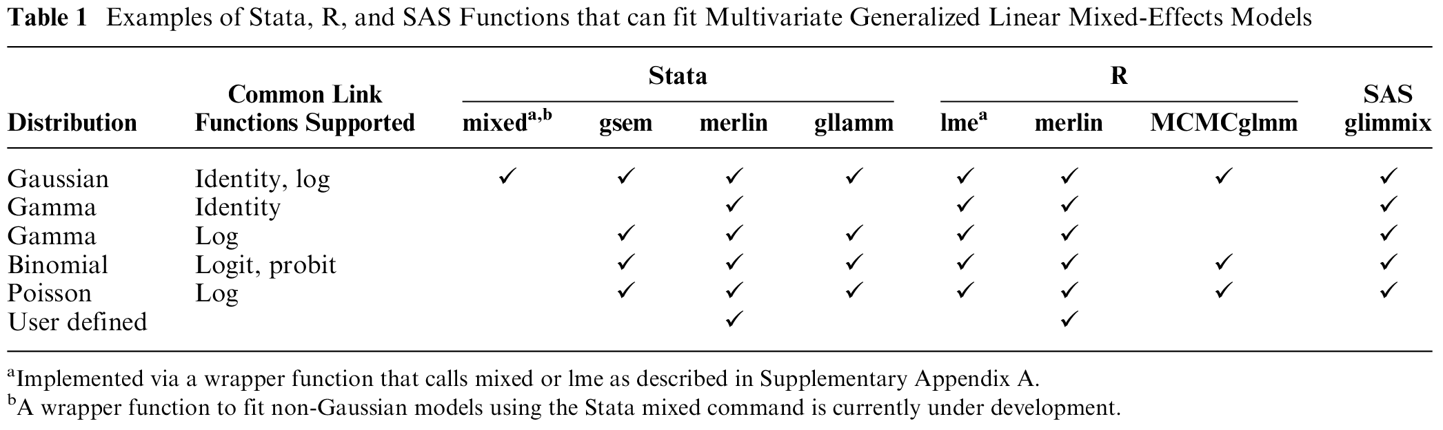
Implemented via a wrapper function that calls mixed or lme as described in Supplementary Appendix A.

A wrapper function to fit non-Gaussian models using the Stata mixed command is currently under development.

Simulation

Simulation Model

We simulated data to represent a 2-arm cluster RCT that recruited a relatively small sample of 200 patients across 10 clusters (study site or country in the case of a multicenter or multinational trial, respectively). In the simulation, we consider a bivariate response $Y_{ij} = {(y_{ij 1}, y_{ij 2})}^{T}$ , with observation $y_{ij 1}$ and $y_{ij 2}$ denoting measurements of total costs and effects, for patient j in cluster i generated from

Y_{ijk} ~ Gamma (μ_{ik}, ϕ_{k})

\log (μ_{ijk}) = β_{0 k} + β_{1 k} \times t_{ij} + b_{ik}, i = 1, 2, \dots, nj = 1, 2, \dots, n_{i} k = 1, 2

(6)

where $E (Y_{ijk}) = μ_{ik}$ is the mean effect observed in the ith cluster of size $n_{i}$ with variance $Var (Y_{ijk}) = σ_{w_{ik}}^{2} = ϕ_{k} μ_{ik}^{2}$ and dispersion $ϕ_{k}$ specific to outcome k (k = 1 for costs and 2 for effects). In a cluster randomized trial, patients in the same cluster receive the same treatment so that $t_{ij}$ is an indicator variable that equals 1 if cluster i receives the new treatment and 0 otherwise. The random-effects $b_{ik}$ are assumed to be drawn from a bivariate normal distribution with mean zero, between-cluster standard variance $σ_{bk}^{2}$ on the log-scale and between-cluster correlation $ρ_{b}$ :

(\begin{matrix} b_{i 1} \\ b_{i 2} \end{matrix}) ~ Normal (0, G = (\begin{matrix} σ_{b 1}^{2} & ρ_{b} σ_{b 1} σ_{b 2} \\ ρ_{b} σ_{b 1} σ_{b 2} & σ_{b 2}^{2} \end{matrix})) i = 1, 2, \dots, M

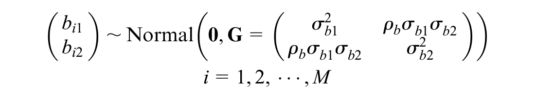
where M is the total number of clusters.

In the simulation, we compared the performance of parameter estimation by maximum likelihood and restricted maximum likelihood via penalized quasi-likelihood in terms of the mean bias, confidence interval coverage, and root mean square error. We assume the true net benefit is £1000 in favor of the new treatment if the cost-effectiveness threshold is £20,000 per unit of effectiveness. Simulated costs and effects from the above model will appear as a right-skewed distributional shape with a lower boundary at zero. This is the distributional shape that is typical of health care costs but is unlike the distributional shape of health utilities (from which quality-adjusted life-years [QALYs] can be derived), which typically appear left skewed. Assuming the effectiveness outcome is the QALY, the simulated effects represent QALYs on a transformed scale, such that the corresponding QALY value on the natural scale of measurement can be obtained by applying a straightforward linear transformation:

QAL Y_{ij} = 1 - rQAL Y_{ij} i = 1, 2, \dots, n j = 1, 2, \dots, n_{i}

(7)

where rQALY_ij is the simulated QALY value for patient j in cluster i and QALY_ij the linear transformation of rQALY_ij to generate the corresponding QALY value that would be observed in practice and left-skewed in distribution.

Simulation Parameters and Algorithm

Parameter values used to inform the simulation specified above were taken from the final case model of a simulation study by Gomes et al.,¹¹ in which the authors assessed the performance of various statistical methods for cost-effectiveness analysis alongside cluster RCTs. The underlying parameter values in the Gomes et al. study were based on a systematic review the authors have undertaken to identify plausible estimates of parameter values for economic evaluation alongside cluster RCTs. Table 1 of their paper summarizes these data and the justification for each value used in their simulation. Because the simulation model in equation (6) is a multiplicative treatment-effect model, each parameter value used in the simulation by Gomes et al. needs to be transformed to generate the corresponding estimate on the logarithmic scale. Table 2 displays the data from Gomes et al. and the corresponding log-transformed value generated for the simulation model above. Based on a description of their simulation, we set $β_{01} = \log (£ 100)$ , $β_{11} = \log (£ 600) - \log (£ 100)$ , $β_{02} = \log (0.125)$ , $β_{12} = \log (0.125) - \log (0.20)$ , representing overall mean incremental costs of £500, incremental mean effects of 0.075, and a mean incremental net monetary benefit of £1000 at a cost-effectiveness threshold of £20,000 per QALY considered by Gomes et al.

Table 2

Parameters Used in the Simulation

Parameter		Final Case (Gomes et al). Natural Scale	Value Used in the Simulation (Log-Scale)	Justification
Total number of clusters	N	30	10	Test performance of methods when number of clusters is small
No. of individuals per cluster	$n_{i}$	50	20	Test performance of methods when sample size is small
Level of imbalance		0.5	0	Set to zero in the present simulation to check the impact of sample size only on performance of estimation procedures
ICC for costs	ICC_c	0.05	0.5	Used only to reconstruct final case of Gomes et al.
ICC for outcomes	ICC_q	0.02	0.02	Used only to reconstruct final case of Gomes et al.
Coefficient of variation (CV) for costs	CV_c	0.5	0.65	Coefficient of variation on log-scale based on reconstructed final case data (Gomes et al. 2012)
Coefficient of variation for outcomes	CV_q	0	0.65	Not reported in Gomes et al. as outcomes modeled using a normal distribution; we reconstructed their data assuming a CV of 0.5
Individual-level correlation of costs and effects	$ρ_{w_{1}}$	−0.2	0	Assumed outcomes are independent given the random effects
Cluster-level correlation	$ρ_{b_{1}}$	0.1	0.1	Justification given in Gomes et al. (2012)
Mean costs placebo	—	—	£100	Mean treatment and control group costs were taken to give a difference of £500 assumed in Gomes et al. (2012)
Mean costs of new treatment	—	—	£600
Mean effects of placebo	—	—	0.8	Mean effects for the treatment and control groups were taken to give a difference of 0.025 assumed in Gomes et al. (2012)
Mean effects of new treatment	—	—	0.875

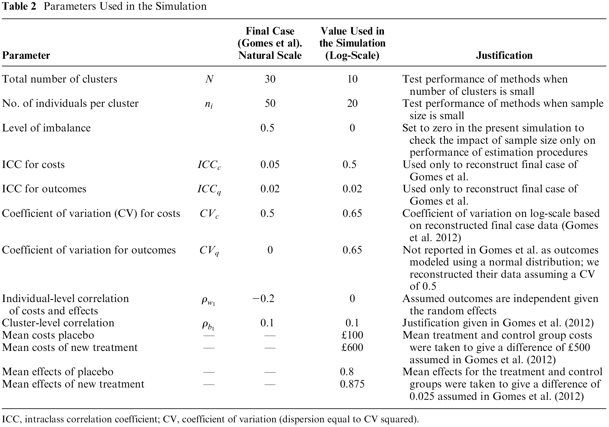
ICC, intraclass correlation coefficient; CV, coefficient of variation (dispersion equal to CV squared).

To derive the required variance and dispersion terms on the log-scale, we first reconstructed the data from Gomes et al. using their additive treatment effects generalized mixed-effects model assuming the errors follow a gamma distribution. From the reconstructed data, we took the logarithm of the patient-level costs and effects (QALYs). We used this log-transformed data to estimate the between-cluster variance (defined as the variance of the cluster-mean costs and cluster mean effects on the log-scale) and the error variance (defined as the mean of the squared within-cluster patient-level errors or deviations). Based on these calculations, we set the between-cluster standard deviations on the log-scale $σ_{b 1} = 0.152$ and $σ_{b 2} = 0.121$ , corresponding to $σ_{b 1} = £ 11.47$ and $σ_{b 2} = 0.014$ on the natural scale of measurement for costs and effects, respectively. Finally, the degree of skewness of the gamma-distributed random variable is a function of the dispersion factor that can be derived from the coefficient of variation. From the reconstructed data, we estimated the coefficient of variation on the log-scale to be 0.65, corresponding to a coefficient of variation of 0.5 assumed for both costs and QALYs on the natural scale of measurement. A step-by-step outline of the simulation algorithm is given below:

Simulate costs and QALYs for a 2-arm cluster RCT from an additive treatment effect generalized mixed-effects model with gamma-distributed error structure based on data from Gomes et al.

Calculate log (costs) and log (QALYs) for each patient and use this to estimate the between-cluster variance $σ_{b}^{2}$ (variance of the cluster means) and the within-cluster or error-variance $σ_{w}^{2}$ on the log-scale.

Estimate the dispersion factor $ϕ$ from the $σ_{w}^{2}$ using the fact that the intraclass correlation coefficient (ICC) of a gamma-distributed random variable on the log-scale is given by $IC C_{gamma - \log} = \frac{σ_{b}^{2}}{σ_{b}^{2} + ψ_{1} (\frac{1}{ϕ})}$ ), where $ψ_{1}$ is the trigamma function, which is the second derivative of the gamma function (Nagakawa et al.⁴²). From the above definition of the ICC, it is clear that $ψ_{1} (\frac{1}{ϕ})$ estimates the error variance $σ_{w}^{2}$ on the log-scale and that the dispersion is given by $ϕ = \frac{1}{ψ_{1}^{- 1} (σ_{w}^{2})}$ , where $ψ_{1}^{- 1}$ is the inverse-trigamma function.

Simulate costs and effects data using the simulation model described by equation (6) based on the parameter values generated in steps 1 to 3 above, and fit the different models to the data. Obtain the parameter vector and the associated covariance matrix from the fitted mixed-effects regression model.

Use Monte Carlo simulation to estimate standard errors and confidence intervals for the incremental costs, incremental effects, and the incremental net benefit on the natural scale of measurement for costs and effectiveness outcomes. This involves generating 1000 replicates of the regression parameters, assuming a multivariate normal distribution for the parameter estimates on the log-scale.

Repeat steps 3 to 5 for a total of 2000 times, each time calculating cost-effectiveness parameters and their associated standard errors and confidence intervals.

We compared the performance of parameter estimation by maximum likelihood and restricted maximum likelihood via penalized quasi-likelihood in terms of the mean bias, confidence interval coverage, and root mean square error, assuming that the true net benefit is £1000 at a cost-effectiveness threshold of £20,000 per QALY or unit of effectiveness. Maximum likelihood estimates were obtained by numerical integration via the gsem function in Stata and by penalized quasi-likelihood via mixed and lme functions in Stata and R, respectively. The vce option in Stata was used to obtain robust estimates of the covariance matrix of the regression parameters in the maximum likelihood models. Restricted maximum likelihood estimates were available only via penalized quasi-likelihood using the mixed and lme functions.

Simulation Results

The simulation results are presented in Table 3 for the base-case parameter values (Table 2) and 3 simulated scenarios. The scenarios tested the performance of the methods when 1) the total number of clusters is decreased from 10 to 5, 2) the cluster size is increased from 20 to 50 individuals, and 3) the coefficient of variation is increased from 0.5 to 1.0, reflecting a higher degree of skewness in distribution (Figure 1). For the base-case simulation with a sample size of 200 individuals recruited across 10 clusters, the mean bias was small in all implementations of the 2 estimation procedures. The restricted maximum likelihood estimates (mean bias ranged from £1.11 to £1.31 assuming the true net benefit is £1000) were, however, less biased on average than the corresponding estimates obtained by maximum likelihood (range in mean bias £3.00 to £5.85; Table 3). Similarly, all models produced 95% confidence interval coverage probabilities greater than 0.90, but the restricted maximum likelihood estimates were closer to the desired 0.95 nominal value than the corresponding coverage probabilities obtained via maximum likelihood.

Figure 1

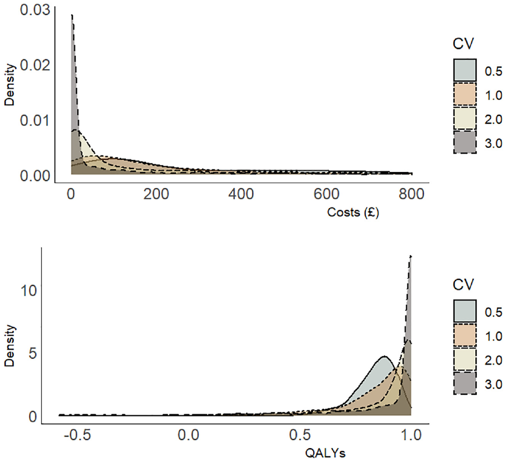
Simulated distribution of costs and quality-adjusted life-years for different coefficients of variation (CVs) defined as the ratio of the standard deviation to the mean.

Table 3

Simulation Results Based on a True Net Monetary Benefit Value of £1000 at a Cost-Effectiveness Threshold of £20,000 per Quality-Adjusted Life-Year

Simulation Parameters and Method	Mean (SE) Bias, £	95% CI Coverage	RMSE, £
Base case simulation (N = 200 from 10 clusters each of size 20, CV = 0.5 for costs and effects, ICC_costs = 0.05, ICC_effects = 0.02)
Stata gsem, ml vce robust	5.85 (13.57)	0.93	331.13
Stata mixed, ml vce robust via pql	3.00 (13.53)	0.93	329.87
Stata mixed, reml via pql	1.31 (13.49)	0.95	329.09
R lme, ml via pql	2.78 (13.52)	0.94	329.79
R lme, reml via pql	1.11 (13.49)	0.96	329.04
Scenario 1 (base case with no. of clusters changed from 10 to 5)
Stata gsem, ml vce robust	6.40 (26.04)	0.82	481.54
Stata mixed, ml vce robust via pql	3.91 (25.97)	0.81	480.22
Stata mixed, reml via pql	4.71 (25.9)	0.96	479.11
R lme, ml via pql	3.94 (25.97)	0.93	480.33
R lme, reml via pql	4.64 (25.9)	0.96	479.11
Scenario 2 (base case with cluster size changed from 20 to 50)
Stata gsem, ml vce robust	0.43 (10.14)	0.92	265.5
Stata mixed, ml vce robust via pql	−1.26 (10.12)	0.92	265.0
Stata mixed, reml via pql	−2.14 (10.11)	0.94	264.7
R lme, ml via pql	−1.44 (10.12)	0.91	264.9
R lme, reml via pql	−2.20 (10.11)	0.94	264.7
Scenario 3 (base case with CV changed from 0.5 to 1.0 for both costs and effects)
Stata gsem, ml vce robust	13.77 (23.42)	0.93	593.9
Stata mixed, ml vce robust via pql	4.73 (23.19)	0.93	588.2
Stata mixed, reml via pql	0.47 (23.09)	0.94	585.9
R lme, ml via pql	4.42 (23.18)	0.93	588.1
R lme, reml via pql	0.31 (23.09)	0.94	585.9

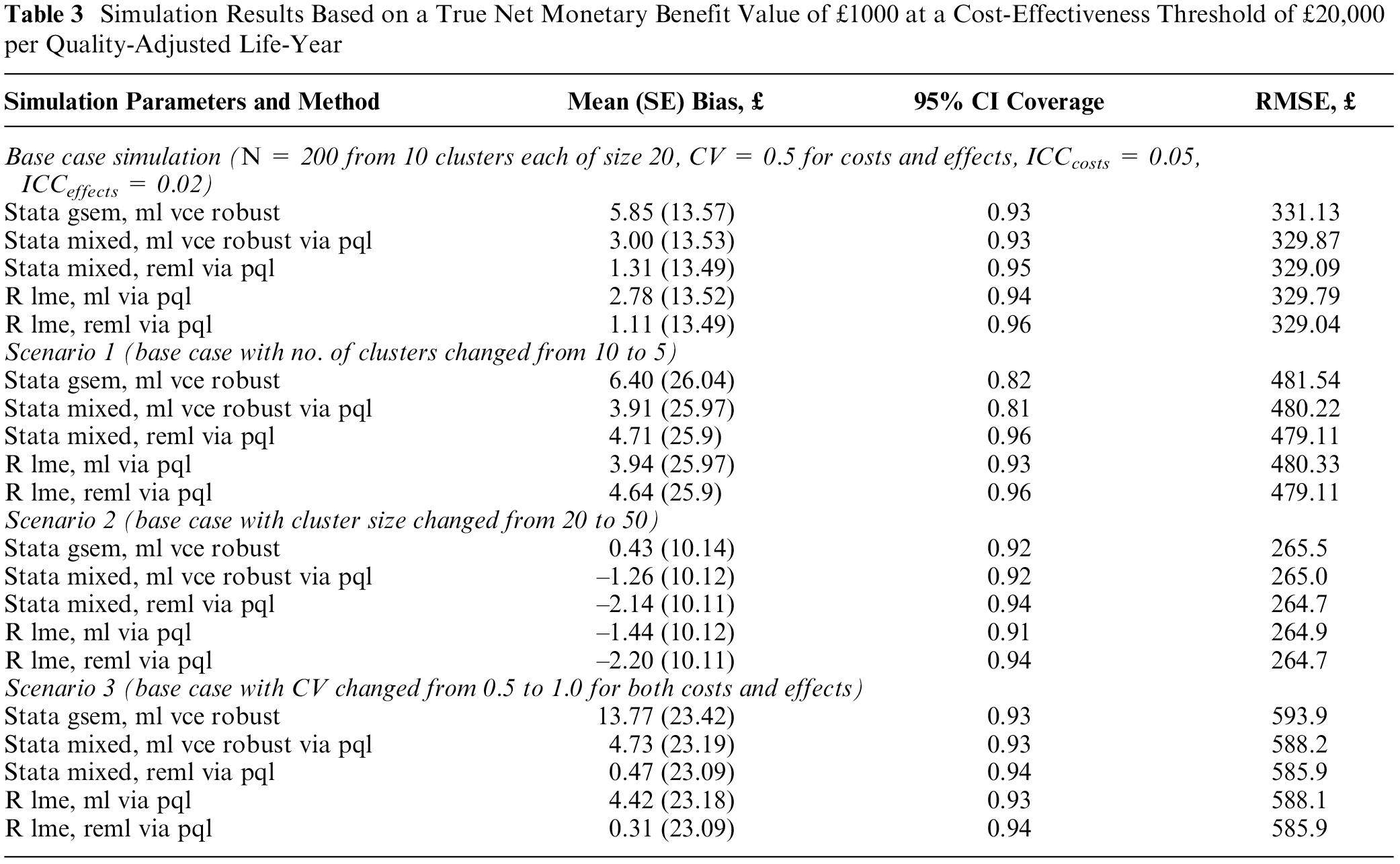
For a reduced sample size of 100 individuals across 5 clusters (scenario 1) of equal size, the estimation bias increased as compared with the base-case simulation assumptions, but the impact on model performance was more pronounced for confidence interval coverage (scenario 1, Table 3). At this small number of clusters and sample size, maximum likelihood generated coverage probabilities that are less than 0.85. In contrast, the coverage in the restricted maximum likelihood models remained relatively unaffected by the reduction in sample size. Figure 2 shows the relationship between model performance and sample size by varying the number of clusters but keeping the cluster size fixed at 20 individuals. Estimation bias decreased toward zero with an increasing number of clusters, and the confidence interval coverage converged to 0.95.

Figure 2

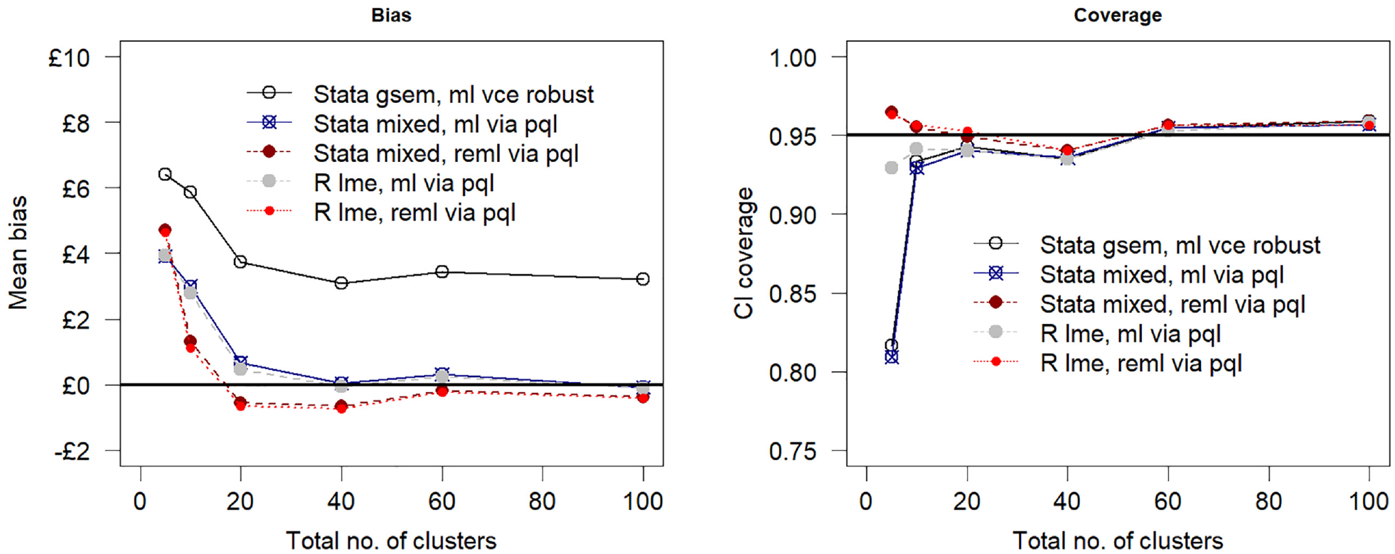
Mean bias and 95% confidence interval (CI) coverage versus number of clusters assuming a true net benefit of £1000 at £20,000 per quality-adjusted life-year cost-effectiveness threshold. PQL, penalized quasi likelihood, ml, maximum likelihood; reml, restricted maximum likelihood estimation.

Increasing the sample size to 500 individuals spread across the 10 clusters by increasing the cluster size to 50 (scenario 2) produced less biased estimates of the incremental net benefit and better confidence coverage for all models as compared with the base-case simulation. Maximum likelihood estimation via the gsem command in Stata was the least biased as compared with maximum likelihood and restricted maximum likelihood estimation by penalized quasi-likelihood. Figure 3 shows the relationship between sample size and model performance when the total number of clusters is fixed at 10. The plot suggests the estimation bias decreases as the sample size is increased by increasing the cluster size from 10 to 100 individuals per cluster, but the confidence interval coverage remains relatively unaffected, falling below the desired nominal 0.95 value coverage value for all tested estimation procedures.

Figure 3

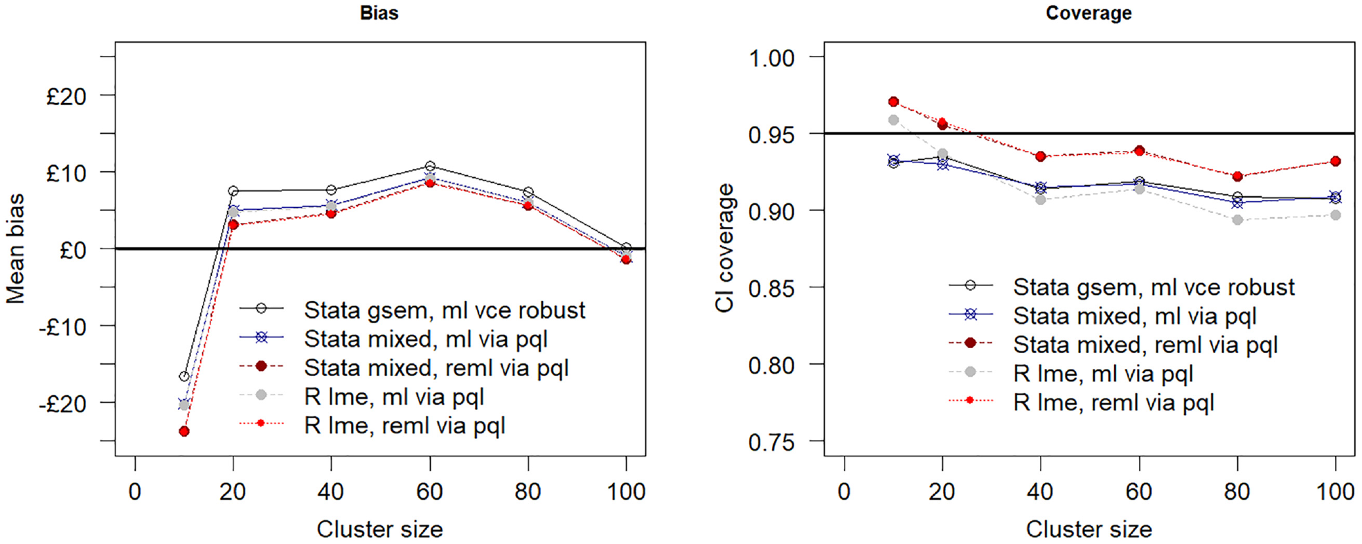
Mean bias assumes a true net benefit of £1000 at £20,000 per quality-adjusted life-year cost-effectiveness threshold and 95% confidence interval (CI) coverage versus cluster size (i.e., number of individuals per cluster). The total number of clusters is fixed at 10. PQL, penalized quasi likelihood; ml, maximum likelihood; reml, restricted maximum likelihood estimation.

In the final simulated scenario, the coefficient of variation was increased from 0.5 (base-case simulation) to 1.0 (scenario 3) to reflect greater skewness in the data (Figure 1) for a sample size of 200 individuals spread equally across 10 clusters. This increased the bias in the estimation of the incremental net benefit by maximum likelihood but decreased the bias in the estimates generated by the restricted maximum likelihood models.

Application to Data from Clinical Trials

Example 1: UK FASHION Trial

UK FASHION was a pragmatic 2 parallel-arm multicenter randomized controlled trial that evaluated the clinical and cost-effectiveness of arthroscopy surgery versus physiotherapy as treatment options for hip pain resulting from femoroacetabular impingement syndrome.⁴³ The trial recruited a total of 348 patients across 23 hospitals and randomly assigned 171 to surgery and 177 to physiotherapy. Participants were followed up for 12 mo, and data were collected prospectively at baseline and at 6 and 12 mo after randomization. The primary outcome was the hip-related quality of life, measured by the International Hip Outcome Tool (iHOT-33),⁴⁴ a validated patient-reported hip-related quality-of-life measure for young, active patients with hip disorders. At each assessment point, participants were asked to report this outcome and their health-related quality of life measured by the EQ-5D-5L and SF-12 version 2, as well as health and social care resource use and costs. The clinical outcomes data were analyzed based on intention-to-treat principles and took the form of a mixed-effects multivariable linear regression that included treatment allocation, impingement type, gender, and baseline scores for relevant outcomes as fixed covariates and a random term for study site.⁴⁵ A prospective within-trial cost-utility analysis was also conducted from a UK National Health Service and Personal Social Services (NHS/PSS) perspective and a 12-mo time horizon.⁴⁵ The base-case analysis closely mirrored the analytic model for the clinical outcomes and took the form of bivariate seemingly unrelated regressions using imputed attributable costs and EQ-5D-generated QALYs as outcomes and treatment allocation, gender, impingement type, and baseline scores as fixed effects. Also, study site was included as a fixed covariate, unlike the clinical outcomes model, which included this variable as a random effect. Including study site as a fixed effect in the economic analysis was done partly for practical reasons and partly because it was not expected a priori for the treatment effect to differ markedly across NHS centers. Further details of the study design, conduct, and findings are available from the published study protocol⁴³ and the main trial paper.⁴⁵

To illustrate the methods outlined in this article, we restrict ourselves to 263 (132 in the surgery group and 131 in the physiotherapy group) of the 348 total trial sample with complete outcome and covariate information for the economic analysis (note that the remaining 85 participants had missing covariates; hence, it was not possible to include these individuals in the regressions). In this illustration, we assigned a nominal total cost value of £1.00 to 2 patients in the physiotherapy group who had reported a zero-cost observation. This was done to avoid problems with zero costs when modeling costs using the gamma distribution as the 2 patients did not receive any intervention or report health and social care service use during the 12 mo of follow-up.

Figure 4 displays the distribution of total costs and QALYs by treatment group during the 12-mo follow-up period. The plots suggest a departure from normality in distribution for both outcomes, with health care costs exhibiting a degree of skewness to the right and QALYs in the opposite direction. Residual diagnostic plots obtained from fitting linear mixed-effects regressions with covariate adjustment are presented in Figure 5. The normal QQ plots do not suggest marked deviations from the normality of the errors, and the scatter plots of the residuals versus fitted values suggest the means of the residuals are not too far from zero to invalidate the results of a normally distributed error fit. However, the scale-location plots suggest the equal variance (homoscedasticity) assumption might be inappropriate for these data.

Figure 4

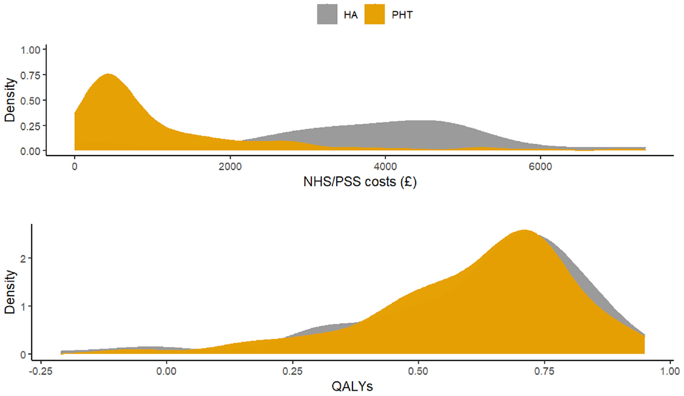
Distribution of total health and social care costs and quality-adjusted life-years accrued over 12 mo of follow-up in the UK Fashion study displayed by treatment group. HA, hip arthroscopy; PHT, personalized hip therapy.

Figure 5

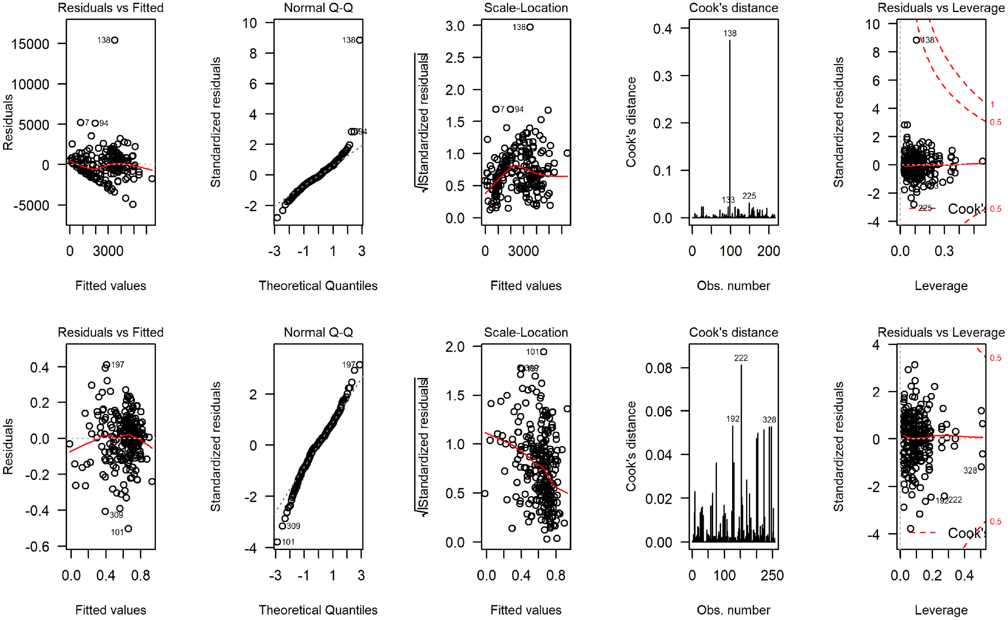
Regression diagnostic plots from fitting normal error regression to total National Health Service/ Personal Social Services costs (4 plots on the top) and quality-adjusted life-years (4 bottom plots) for the UK FASHION study.

Nevertheless, to illustrate the methods presented here, we fit 3 bivariate mixed-effects random intercept models with treatment allocation, gender, impingement type, baseline costs (cost model), and baseline health-related quality-of-life scores (QALYs model) as fixed effects and study site as a random effect. In the first 2 models, a normal distribution with identity link function was assumed for QALYs, but costs were modeled using normal and gamma distributions with identity and log-link functions, respectively. In the third model, the distribution of QALYs was converted from left skew to right skew by applying the transformation specified in equation (7). Costs and the transformed QALY variable were then jointly modeled assuming a gamma distribution with log-link function similar to the simulation model specified in equation (6). Note that because equation (7) maps values from left to right, individuals with higher QALYs on the untransformed (observed QALY scale) will have lower values on the transformed scale and vice versa. Therefore, parameter estimates should be interpreted with care. In particular, estimates of the treatment effect on the transformed QALY scale when modeled using gamma regression (equation (6)) should be reversed such that the treatment effect favoring active/new treatment on the transformed scale should favor the control on the untransformed scale and vice versa.

The results for the FASHION data are presented in Table 4. Estimates of incremental costs and incremental QALYs were broadly similar across platforms and estimation procedures. The associated standard errors of the incremental costs estimated by different packages were also similar across statistical software packages and platforms with maximum likelihood, generally producing smaller standard errors than the restricted maximum likelihood and the WinBUGS implementations. The model that assumed normally distributed errors for costs and QALYs (model F1) generated mean (standard error) incremental costs ranging from £2573 (£198) to £2609 (£249) and incremental QALYs ranging from −0.012 (0.0184) to −0.025 (0.026) in the WinBUGS model. Parameter estimates from model F2 and F3 in which the costs were modeled using a gamma distribution with log link are additive on the log-scale and multiplicative on the natural scale of measurement. Therefore, log-cost and log-QALY differences generated from the 2 models were combined with the intercept-term for each outcome and back-transformed to generate incremental costs and incremental QALYs for surgery as compared with physiotherapy on the natural scale of measurement.⁴⁶ This produced incremental costs ranging from £3220 (£584) to £3281 (£567) and incremental QALYs ranging from 0.0036 (0.019) to 0.0012 (0.042) in favor of the surgery.

Table 4

Illustrated Example from Clinical Trials Using the UK FASHION Trial Data (Random-Intercepts Model)^a

Model	Package, Function, and Method of Estimation	Difference in Mean Costs (SE), £	Difference in Mean QALYs (SE)
Model F1: bivariate mixed-effects regression withCosts ∼ normalQALYs ∼ normal	Stata mixed, ml via PQL	2575 (196)	−0.012 (0.0184)
	Stata mixed, reml via PQL	2573 (198)	−0.012 (0.0187)
	Stata merlin, ml	2597 (193)	−0.012 (0.018)
	Stata gsem, ml	2601 (194)	−0.013 (0.019)
	R lme, ml via PQL	2600 (194)	−0.010 (0.019)
	R lme, reml via PQL	2600 (197)	−0.010 (0.019)
	WinBUGS MCMC	2609 (249)	−0.025 (0.026)
Model F2: Bivariate mixed-effects regression withCosts ∼ gamma (link = log)QALYs ∼ normal	Stata mixed, ml via PLQ	3192 (357)	−0.011 (0.0799)
	Stata mixed, reml via PQL	3178 (352)	−0.011 (0.0825)
	Stata merlin, ml	3246 (484)	−0.013 (0.019)
	Stata gsem, ml	3246 (483)	−0.012 (0.019)
	R lme, ml via PQL	3246 (483)	−0.013 (0.019)
	R lme, reml via PQL	3248 (490)	−0.013 (0.019)
	WinBUGS MCMC	3220 (584)	−0.013 (0.019)
Model F3: Bivariate mixed-effects regression withCosts ∼ gamma (link = log)1-QALYs ∼ gamma (link = log)	Stata mixed, ml via PQL	3223 (383)	0.00092 (0.0072)
	Stata mixed, reml via PQL	3212 (387)	0.00089 (0.0073)
	Stata merlin, ml
	Stata gsem, ml robust se	3227 (557)	0.0012 (0.042)
	R lme, ml via PQL	3247 (489)	0.0037 (0.019)
	R lme, reml via PQL	3247 (497)	0.0036 (0.019)

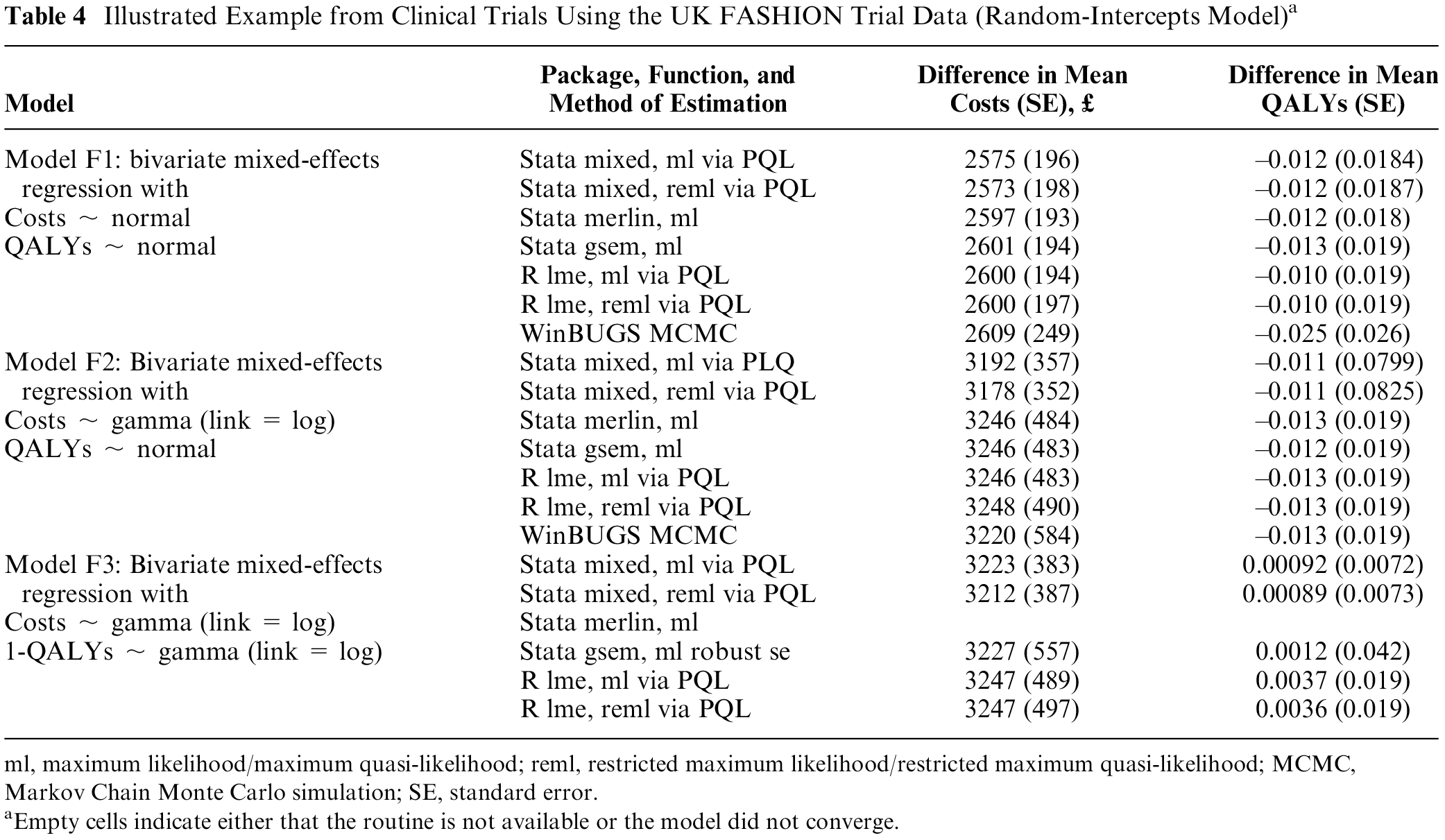
ml, maximum likelihood/maximum quasi-likelihood; reml, restricted maximum likelihood/restricted maximum quasi-likelihood; MCMC, Markov Chain Monte Carlo simulation; SE, standard error.

Empty cells indicate either that the routine is not available or the model did not converge.

Example 2: GRACE Trial

GRACE was a multinational, randomized placebo-controlled trial that assessed the clinical and cost-effectiveness of amoxicillin for acute lower respiratory tract infection in people aged 60 y or older.^47,48 Two thousand sixty patients were recruited from primary care practices in 12 European countries (Belgium, England, France, Germany, Italy, the Netherlands, Poland, Slovakia, Slovenia, Spain, Sweden, and Wales) and randomized to amoxicillin (n = 1037) or placebo (n = 1023). Follow-up was 28 d from randomization. The primary clinical outcome was the duration of symptoms dichotomized to generate a binary response, reflecting mild to moderate versus severe cough. Cost-effectiveness was assessed from the perspective of society with costs expressed in Euros and in 2012 prices. QALYs were calculated from EQ-5D-3L data collected at baseline and weekly over the 28-d follow-up period. The trial methods, results, and the subsequent economic evaluation are published elsewhere.^47,48 We use the GRACE data here to illustrate simultaneous modeling of 3 outcomes (costs, QALYs, and proportion with a severe cough), each of which is of a different data form. These types of analyses can be useful for economic evaluations conducted alongside multinational, multicenter, or cluster randomized controlled trials, where the aim is to express cost-effectiveness using alternative measures of benefit or effectiveness. For example, cost-effectiveness and cost-utility analyses can be conducted simultaneously in a single analytic model. If outcomes are sufficiently correlated, there may be gains in precision from modeling the between-outcome and between-cluster correlations.

Figure 6 displays the distribution of total costs and QALYs accrued over the 28-d follow-up by treatment group. The plots suggest a departure from normality in distribution for both outcomes, with health care costs exhibiting the typical skewness to the right and QALYs in the opposite direction. The scale-location plots show evidence of heteroscedasticity, suggesting the constant variance assumption implied in a linear mixed-effects model may be inappropriate for the GRACE data (Figure 7). We fit 3 trivariate mixed-effects random coefficient regressions with treatment allocation, age, gender, and baseline utility as fixed-effect covariates and study country as random effect. In the first analysis (model G1), we assumed costs and QALYs follow a normal distribution, whereas the severity of cough was modeled using a binomial distribution. For the second model (model G2), costs were modeled using a gamma distribution with a log link function to accommodate skewness in the data, whereas the distributions for QALYs and severity of cough remained the same as in model G1. The third model assumed that costs and QALYs follow a gamma distribution with the transformation implied by equation (7) applied to the QALY variable.

Figure 6

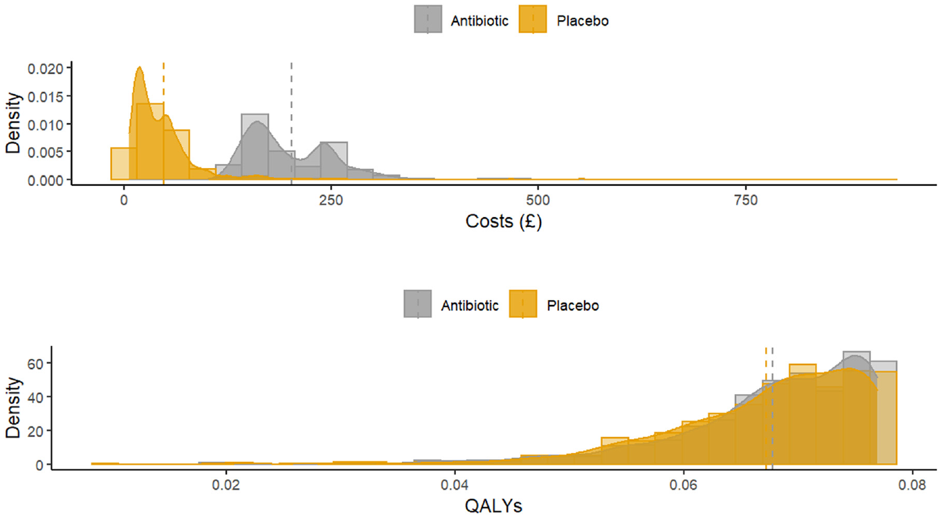
Distribution of costs and quality-adjusted life-years accrued over 28 d displayed by treatment group.

Figure 7

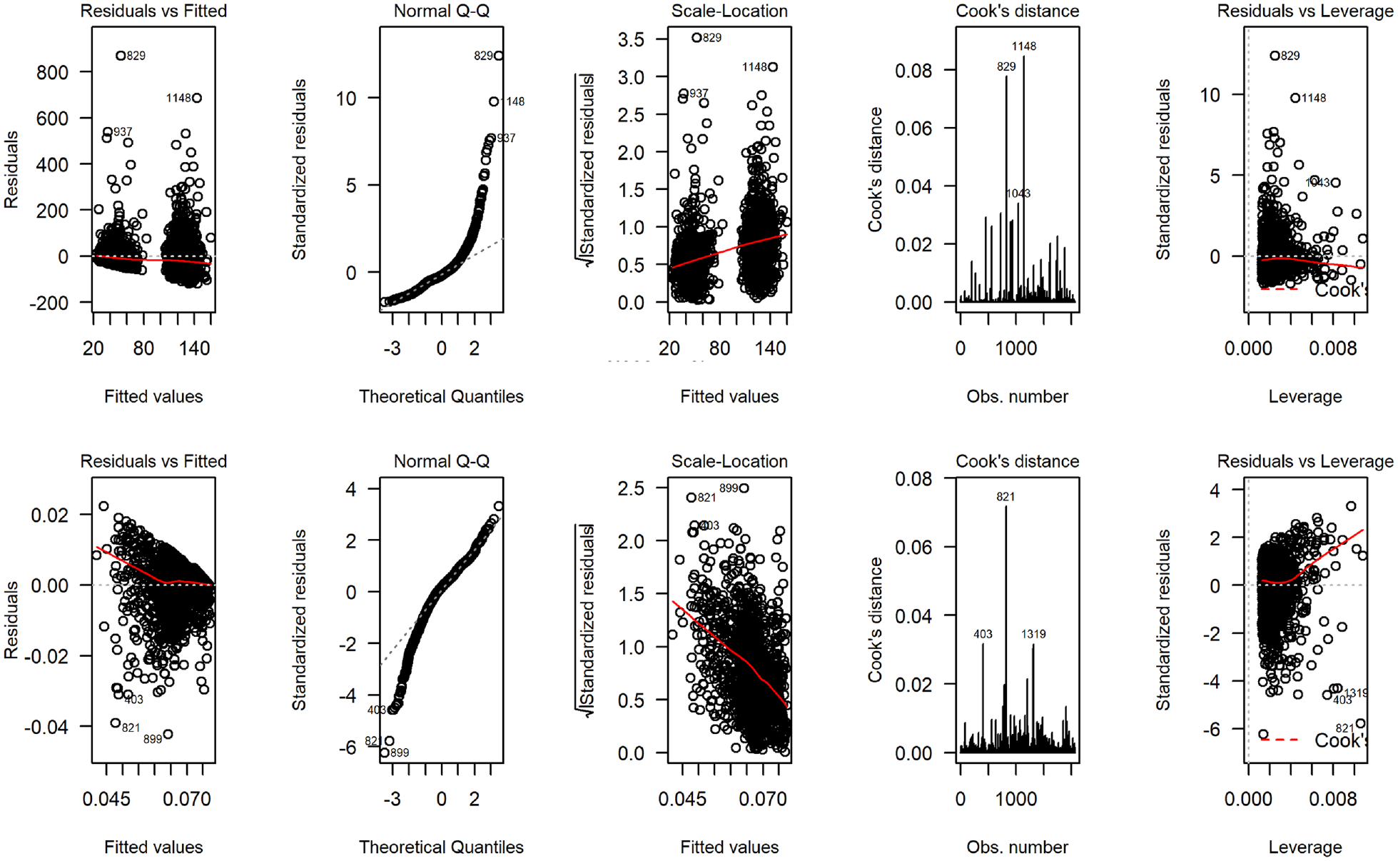
Diagnostic plots from fitting normal error regression to total costs (4 plots on the top) and quality-adjusted life-years (4 bottom plots) for the GRACE study.

Adjusted estimates of the incremental mean costs, incremental mean QALYs, and an incremental mean reduction in the proportion with a severe cough for amoxicillin compared with placebo, together with the associated standard errors from fitting these models, are presented in Table 5. Estimates of incremental costs and incremental QALYs and the corresponding standard errors were broadly similar across alternative estimation procedures. In this example, the sample size of 2060 patients from 12 countries is large, such that all 3 estimation procedures (maximum likelihood, restricted maximum likelihood, and the Bayesian MCMC implementation) produced similar estimates of the standard errors associated with incremental costs and incremental outcomes.

Table 5

Illustrated Example from Multinational Clinical Trial with 3 Outcomes Using GRACE Data (Random-Coefficient Model)^a

Model	Package, Function, and Method of Estimation	Incremental Costs; Mean (SE), €	Incremental QALYs; Mean (SE)	Incremental Proportion with Severe Cough (SE)
Model G1: Bivariate mixed-effects regression withCosts ∼ normalQALYs ∼ normalCough ∼ binomial (link = log)	Stata mixed, ml
	Stata mixed, reml
	Stata merlin, ml	154.34 (2.70)	0.0003 (0.0310)	−0.0202 (0.0138)
	Stata gsem, ml	154.34 (2.69)	0.0003 (0.0312)	−0.0202 (0.0140)
	R lme, ml via PQL	154.34 (2.71)	0.0003 (0.0311)	−0.0202 (0.0137)
	R lme, reml via PQL	135.87 (11.22)	0.0003 (0.0312)	−0.0202 (0.0137)
	WinBUGS MCMC	131.90 (14.59)	0.0004 (0.0007)	−0.0046 (0.0291)
Model G2: Bivariate mixed-effects regression withCosts ∼ gamma (link = log)QALYs ∼ normalCough ∼ binomial (link = logit)	Stata mixed, ml via PQL
	Stata mixed, reml via PQL
	Stata merlin, ml	108.97 (14.36)	0.0003 (0.0311)	−0.0044 (0.0227)
	Stata gsem, ml	108.96 (14.36)	0.0003 (0.0311)	−0.0044 (0.0227)
	R lme, ml via PQL	108.96 (14.36)	0.0003 (0.0311)	−0.0044 (0.0227)
	R lme, reml via PQL	107.65 (14.41)	0.0003 (0.0311)	−0.0018 (0.0259)
	WinBUGS MCMC	113.00 (13.21)	0.0002 (0.0005)	−0.0073 (0.0267)
Model G3: Bivariate mixed-effects regression withCosts ∼ normal1. QALYs ∼ gamma (link = log)Cough ∼ binomial (link = log)	Stata mixed, ml via PQL
	Stata mixed, reml via PQL
	Stata merlin, ml
	Stata gsem, ml
	R lme, ml via PQL	108 (1400)	0.0002 (0.062)	−0.0040 (0.02278)
	R lme, reml via PQL	108 (14.39)	0.0002 (0.062)	−0.0011 (0.02605)
	WinBUGS MCMC	107 (12.65)	−0.0001 (0.0047)	−0.0090 (0.0282)

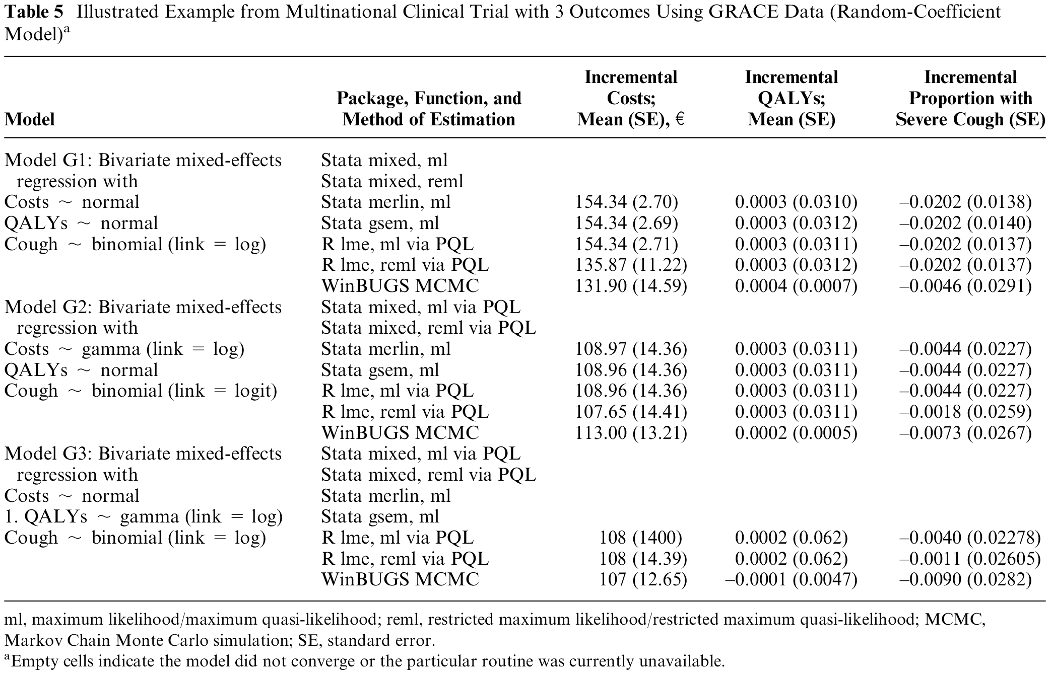
ml, maximum likelihood/maximum quasi-likelihood; reml, restricted maximum likelihood/restricted maximum quasi-likelihood; MCMC, Markov Chain Monte Carlo simulation; SE, standard error.

Empty cells indicate the model did not converge or the particular routine was currently unavailable.

To illustrate the impact of alternative distributional assumptions on within-trial cost-effectiveness, we changed the distribution of costs (a normal distribution in model G1 to a gamma distribution with log-link in models G2 and G3) while maintaining the same distributional assumptions for QALYs and the probability of severe cough. This has minimal impact on incremental QALYs but changed the incremental mean costs from €135.87 (standard error €11.22) in model G1 to €107.65 (standard error €14.41) in model G2 and €108 (standard error €14.41) in model G3. For this particular example, the distribution of health care costs was skewed to the right, the model with gamma-distributed error structure produced a lower estimate of the mean cost difference compared with assuming a normal distribution for the costs.

Discussion

In this article, we have shown how the generalized linear mixed-model framework may be extended to model multiple outcomes of mixed data types typically encountered in many health economic investigations. We developed easily implementable tools to estimate the models in the statistical programming packages Stata and R and illustrated their applications using observed and simulated data from clinical trials. These models may be usefully employed, for example, as part of sensitivity analyses to assess the robustness of multinational and cluster randomized trial–based cost-effectiveness analyses for departures from assumed normality of the error structure. The new tools will also make it possible to implement methods in Stata and R for cost-effectiveness analyses that use data from multinational trials (previously proposed and implemented in WinBUGS and MLwiN^8,9,49,50) for normally and nonnormally distributed data. Thus, the proposed methods can be employed to assess the generalizability of cost-effectiveness results from multinational trials where concerns about between-country heterogeneity in health care resource use, costs, and preference-based health outcome measures (see, for example^{13,17,54–56} for a detailed discussion of these issues) makes it increasingly unrealistic to pool health care costs across countries directly.

The new methods permit restricted maximum likelihood estimation of a mixed-effects regression with more than 1 dependent variable via a penalized quasi-likelihood algorithm. This may be advantageous in small to moderate sample size applications, as demonstrated in our simulations, in which restricted maximum likelihood was found to produce 95% confidence intervals with better coverage probabilities than maximum likelihood estimation. Our simulations suggest that in studies with moderate sample sizes of 200 individuals spread equally across 10 clusters, both maximum likelihood and restricted maximum likelihood generated estimates of incremental net benefit with low bias but only restricted maximum likelihood produced 95% confidence intervals with coverage probabilities close to the desired 0.95 normal value. Estimation bias increased when the sample size was decreased to 100 individuals spread equally across 5 clusters, but the confidence interval coverage generated via restricted maximum likelihood remained relatively unaffected (scenario 1, Table 3).

Preliminary results from the simulation and applications to the observed clinical trial data also suggest that the new routines produced broadly similar point estimates of parameter values as compared with estimates obtained from Stata’s merlin and gsem and the Bayesian implementation in WinBUGS. Estimates of variance components and standard errors of parameter values were broadly comparable across platforms when the same method of estimation was used, and the data set was relatively large both in terms of the number of clusters and number of individuals per cluster. However, as shown in the simulation, for small to moderate sample size applications (i.e., 100 to 200 patients recruited across 5 to 10 clusters), maximum likelihood can underestimate the variance components (confidence intervals and standard errors around parameter values) as compared with restricted maximum likelihood. Underestimation of variance components will propagate toward underestimation of the uncertainty around final economic endpoints of interest and therefore has implications for characterizing uncertainty in cost-effectiveness analysis. This is important in trial-based economic evaluations as clinical trials often recruit from a relatively small number of study sites, centers, or clusters.

The methods outlined in this article are not novel in that they are based on extensions of pseudo and quasi-likelihood linearization methods^25,26 proposed over 2 to 3 decades ago. However, the implementation in R and Stata for modeling mixed outcomes and applications to the analysis of economic data from clinical trials is a novel and useful addition to the tools available for analysts working in clinical trials research. The new routines are easy to implement and can estimate variances and standard errors by restricted maximum likelihood that are useful for generating confidence intervals with desired coverage in small-sample situations but unavailable in gllamm, merlin, and gsem, which implement more accurate numerical integration techniques. For more complex problems, these other functions may therefore have advantages in being able to estimate the model more accurately. In the meantime, further simulation-based research is required to understand their statistical properties and performance under different modeling assumptions such as in applications involving clusters of unequal sizes and alternative specification of the error structure and link functions.

The parameterizations outlined in the Methods section require data in long format for the analysis, with outcome measures stacked on top of one another to form a single response. This parameterization ensures that individuals with partially observed outcomes data (such as missing costs but not clinical outcomes) can be included in the analysis under the missing-at-random assumption, in which covariate information is fully observed. Case-wise deletion of partially observed outcome data is avoided in this case, and imputation is not required under the missing-at-random assumption, similar to the full information maximum likelihood approach of structural equation modeling (see, for example, Mehta and Neale⁵⁰ and the references therein). Further research should focus on identifying strategies for handling more complex missing data problems such as missing covariates and nonignorable missingness problems in which explicit modeling of the missingness mechanism may need to take into account hierarchical structures within the data.

Finally, cost-effectiveness analysis requires estimates of incremental costs and incremental benefits in the natural unit of measurement. Except for modeling on the identity link scale, estimates of incremental costs and effects generated on the scale of the link function should be transformed back onto the natural scale of measurement for use in cost-effectiveness analysis. This can be achieved by taking random draws from the joint distribution of the parameter estimates on the scale of the link function and then back-transforming the simulated output onto the natural scale of measurement.

Supplemental Material

sj-do-2-mdm-10.1177_0272989X211003880 – Supplemental material for Multivariate Generalized Linear Mixed-Effects Models for the Analysis of Clinical Trial–Based Cost-Effectiveness Data

Supplemental material, sj-do-2-mdm-10.1177_0272989X211003880 for Multivariate Generalized Linear Mixed-Effects Models for the Analysis of Clinical Trial–Based Cost-Effectiveness Data by Felix Achana, Daniel Gallacher, Raymond Oppong, Sungwook Kim, Stavros Petrou, James Mason and Michael Crowther in Medical Decision Making

Supplemental Material

sj-do-3-mdm-10.1177_0272989X211003880 – Supplemental material for Multivariate Generalized Linear Mixed-Effects Models for the Analysis of Clinical Trial–Based Cost-Effectiveness Data

Supplemental material, sj-do-3-mdm-10.1177_0272989X211003880 for Multivariate Generalized Linear Mixed-Effects Models for the Analysis of Clinical Trial–Based Cost-Effectiveness Data by Felix Achana, Daniel Gallacher, Raymond Oppong, Sungwook Kim, Stavros Petrou, James Mason and Michael Crowther in Medical Decision Making

Supplemental Material

sj-do-4-mdm-10.1177_0272989X211003880 – Supplemental material for Multivariate Generalized Linear Mixed-Effects Models for the Analysis of Clinical Trial–Based Cost-Effectiveness Data

Supplemental material, sj-do-4-mdm-10.1177_0272989X211003880 for Multivariate Generalized Linear Mixed-Effects Models for the Analysis of Clinical Trial–Based Cost-Effectiveness Data by Felix Achana, Daniel Gallacher, Raymond Oppong, Sungwook Kim, Stavros Petrou, James Mason and Michael Crowther in Medical Decision Making

Supplemental Material

sj-docx-1-mdm-10.1177_0272989X211003880 – Supplemental material for Multivariate Generalized Linear Mixed-Effects Models for the Analysis of Clinical Trial–Based Cost-Effectiveness Data

Supplemental material, sj-docx-1-mdm-10.1177_0272989X211003880 for Multivariate Generalized Linear Mixed-Effects Models for the Analysis of Clinical Trial–Based Cost-Effectiveness Data by Felix Achana, Daniel Gallacher, Raymond Oppong, Sungwook Kim, Stavros Petrou, James Mason and Michael Crowther in Medical Decision Making

Supplemental Material

sj-R-5-mdm-10.1177_0272989X211003880 – Supplemental material for Multivariate Generalized Linear Mixed-Effects Models for the Analysis of Clinical Trial–Based Cost-Effectiveness Data

Supplemental material, sj-R-5-mdm-10.1177_0272989X211003880 for Multivariate Generalized Linear Mixed-Effects Models for the Analysis of Clinical Trial–Based Cost-Effectiveness Data by Felix Achana, Daniel Gallacher, Raymond Oppong, Sungwook Kim, Stavros Petrou, James Mason and Michael Crowther in Medical Decision Making

Footnotes

The authors declared no potential conflicts of interest with respect to the research, authorship, and/or publication of this article.

The authors disclosed receipt of the following financial support for the research, authorship, and/or publication of this article: Financial support for this study was provided in part by a contract with the University of Warwick and the University of Oxford. The funding agreement ensured the authors’ independence in designing the study, interpreting the data, writing, and publishing the report.

ORCID iDs

Felix Achana

Daniel Gallacher

Raymond Oppong

Sungwook Kim

Supplemental Material

Supplementary material for this article is available on the Medical Decision Making website at .

References

Glick

Doshi

Sonnad

Polsky

Economic Evaluation in Clinical Trials. 2nd ed.Vol. 2 In: Gray

Briggs

, eds. Handbooks in Health Economic Evaluation. Oxford: Oxford University Press; 2015.

Petrou

Gray

Economic evaluation alongside randomised controlled trials: design, conduct, analysis, and reporting. BMJ. 2011;342:d1548.

Gelman

Analysis of variance: why it is more important than ever. Ann Stat. 2005;33(1):1–31.

Henningsen

Hamann

JD.

systemfit: a Package for estimating systems of simultaneous equations in R. J Stat Softw. 2007;23:i04.

Alam

An efficient algorithm for the pseudo likelihood estimation of the generalized linear mixed models (GLMM) with correlated random effects. 2009. Available from: https://www.oru.se/globalassets/oru-sv/institutioner/hh/workingpapers/workingpapers2009/wp-4-2009.pdf. Accessed May 6, 2018.

SAS Institute. SAS/STAT® 9.2 User’s Guide: The GLIMMIX Procedure. 2009. Available from: https://support.sas.com/documentation/cdl/en/statugglmmix/61788/PDF/default/statugglmmix.pdf. Accessed May 9, 2018.

Grieve

Nixon

Thompson

Normand

Using multilevel models for assessing the variability of multinational resource use and cost data. Health Econ. 2005;14(2):185–96.

Manca

Lambert

Sculpher

Rice

Cost-effectiveness analysis using data from multinational trials: the use of bivariate hierarchical modeling. Med Decis Making. 2007;27(4):471–90.

Manca

Rice

Sculpher

Briggs

AH.

Assessing generalisability by location in trial-based cost-effectiveness analysis: the use of multilevel models. Health Econ, 2005;14(5):471–85.

10.

Gomes

Grieve

Nixon

Edmunds

WJ.

Statistical methods for cost-effectiveness analyses that use data from cluster randomized trials: a systematic review and checklist for critical appraisal. Med Decis Making. 2012;32(1):209–20.

11.

Gomes

Grieve

Nixon

Carpenter

Thompson

SG.

Developing appropriate methods for cost-effectiveness analysis of cluster randomized trials. Med Decis Making. 2012;32(2):350–61.

12.

Diaz-Ordaz

Grieve

Nixon

Thompson

Carpenter

JR.

Multilevel models for cost-effectiveness analyses that use cluster randomised trial data: an approach to model choice. Stat Methods Med Res. 2016;25(5):2036–52.

13.

Willan

Pinto

O’Brien

, et al. Country specific cost comparisons from multinational clinical trials using empirical Bayesian shrinkage estimation: the Canadian ASSENT-3 economic analysis. Health Econ. 2005;14(4):327–38.

14.

Baio

Bayesian methods in health economics. In: Chow

S-C

, ed. Chapman & Hall/CRC Biostatistics Series. Boca Raton (FL): Chapman & Hall; 2013.

15.

Cooper

Lambert

Abrams

Sutton

AJ.

Predicting costs over time using Bayesian Markov chain Monte Carlo methods: an application to early inflammatory polyarthritis. Health Econ. 2007;16(1):37–56.

16.

Spiegelhalter

Thomas

Best

Lunn

WinBUGS User Manual. Version 1.4. January 2003. Upgraded to Version 1.4.3. 2007. Available from: https://www.mrc-bsu.cam.ac.uk/wp-content/uploads/manual14.pdf

17.

Plummer

JAGS: a program for analysis of Bayesian graphical models using Gibbs sampling. Distributed Statistical Computing Working Papers. 2003. Available from: http://citeseerx.ist.psu.edu/viewdoc/download?doi=10.1.1.13.3406&rep=rep1&type=pdf. Accessed April 19, 2018.

18.

Charlton

Rasbash

Browne

Healy

Cameron

MLwiN. Version 3.00. Bristol (UK): Centre for Multilevel Modelling, University of Bristol; 2017.

19.

Efron

Better bootstrap confidence intervals. J Am Stat Assoc. 1987;82(397):171–85.

20.

Stata Corporation. Stata Structural Equation Modeling Reference Manual. Release 15. 2017. Available from: https://www.stata.com/manuals/sem.pdf. Accessed May 6, 2018.

21.

Martin

Gasparini

Crowther

Mixed effects regression for linear, non-linear and user-defined models. 2020. Available from: https://cran.r-project.org/web/packages/merlin/merlin.pdf. Accessed May 5, 2020.

22.

Crowther

Extended multivariate generalised linear and non-linear mixed effects models. 2017. Available from: https://arxiv.org/pdf/1710.02223.pdf. Accessed May 6, 2018.

23.

Harville

DA.

Maximum likelihood approaches to variance component estimation and to related problems. J Am Stat Assoc. 1977;72(358):320–38.

24.

Patterson

Thompson

Recovery of inter-block information when block sizes are unequal. Biometrika. 1971;58(3):545–54.

25.

Breslow

Clayton

DG.

Approximate inference in generalized linear mixed models. J Am Stat Assoc. 1993;88(421):9–25.

26.

Wolfinger

O’Connell

Generalized linear mixed models a pseudo-likelihood approach. J Stat Comput Simul. 1993;48(3–4):233–43.

27.

Lindstrom

Bates

DM.

Nonlinear mixed effects models for repeated measures data. Biometrics. 1990;46(3):673–87.

28.

Pinheiro

Bates

DebRoy

, et al. nlme: Linear and Nonlinear Mixed Effects Models. R package version 3.1-137. 2018. Available from: https://CRAN.R-project.org/package=nlme

29.

Venables

Ripley

BD.

Modern Applied Statistics with S. 4th ed. In: Statistics and Computing. New York: Springer; 2002.

30.

Laird

Ware

HJ.

Random-effects models for longitudinal data. Biometrics. 1983l;38:963–74.

31.

Lindstrom

Bates

DM.

Newton–Raphson and EM algorithms for linear mixed-effects models for repeated-measures data. J Am Stat Assoc. 1988;83(404):1014–22.

32.

Pinheiro

Bates

DM.

Mixed-Effects Models in S and S-PLUS. New York: Springer; 2000.

33.

Raudenbush

Bryk

AS.

Hierarchical Linear Models: Applications and Data Analysis Methods. 2nd ed. In: Advanced Quantitative Techniques in Social SciencesThousand Oaks (CA): Sage; 2002.

34.

Goldstein

Multilevel Models in Education and Social Research. London: Charles Griffin & Co; 1987.

35.

Hadfield

JD.

MCMC methods for multi-response generalized linear mixed models: the MCMCglmm R package. J Stat Softw. 2010;33(2):1–22.

36.

McCullagh

Nelder

Generalized Linear Models. 2nd ed. London: Chapman and Hall; 1989.

37.

Gueorguieva

Agresti

A correlated probit model for joint modeling of clustered binary and continuous responses. J Am Stat Assoc. 2001;96(455):1102–12.

38.

Gueorguieva

A multivariate generalized linear mixed model for joint modelling of clustered outcomes in the exponential family. Stat Model. 2001;1(3):177–93.

39.

Liang

K-Y

Zeger

SL.

Longitudinal data analysis using generalized linear models. Biometrika. 1986;73(1):13–22.

40.

StataCorp. Stata Statistical Software: Release 15. College Station (TX): StataCorp LLC; 2017.

41.

SAS Institute. SAS/STAT 9.3 User’s Guide: The GLIMMIX Procedure. 2011. Available from: https://support.sas.com/documentation/cdl/en/statug/63962/HTML/default/viewer.htm. Accessed April 19, 2018.

42.

Nakagawa

Johnson

PCD

Schielzeth

The coefficient of determination R² and intra-class correlation coefficient from generalized linear mixed-effects models revisited and expanded. J R Soc Interface. 2017;14(134):20170213.

43.

Griffin

Dickenson

Wall

PDH

, et al. Protocol for a multicentre, parallel-arm, 12-month, randomised, controlled trial of arthroscopic surgery versus conservative care for femoroacetabular impingement syndrome (FASHIoN). BMJ Open. 2016;6(8):e012453.

44.

Mohtadi

NGH

Griffin

Pedersen

, et al. The development and validation of a self-administered quality-of-life outcome measure for young, active patients with symptomatic hip disease: the International Hip Outcome Tool (iHOT-33). Arthroscopy. 2012;28(5):595–610.e1.

45.

Griffin

Dickenson

Wall

PDH

, et al. Hip arthroscopy versus best conservative care for the treatment of femoroacetabular impingement syndrome (UK FASHIoN): a multicentre randomised controlled trial. Lancet. 2018;391(10136):2225–35.

46.

Basu

Rathouz

PJ.

Estimating marginal and incremental effects on health outcomes using flexible link and variance function models. Biostatistics. 2005;6(1):93–109.

47.

Little

Stuart

Moore

, et al. Amoxicillin for acute lower-respiratory-tract infection in primary care when pneumonia is not suspected: a 12-country, randomised, placebo-controlled trial. Lancet Infect Dis. 2013;13(2):123–9.

48.

Oppong

Smith

Little

, et al. Cost effectiveness of amoxicillin for lower respiratory tract infections in primary care: an economic evaluation accounting for the cost of antimicrobial resistance. Br J Gen Pract. 2016;66(650):e633–9.

49.

Pinto

Willan

O’Brien

BJ.

Cost-effectiveness analysis for multinational clinical trials. Stat Med. 2005;24(13):1965–82.

50.

Mehta

Neale

MC.

People are variables too: multilevel structural equations modeling. Psychol Methods. 2005;10(3):259–84.

Supplementary Material

Please find the following supplemental material available below.

For Open Access articles published under a Creative Commons License, all supplemental material carries the same license as the article it is associated with.

For non-Open Access articles published, all supplemental material carries a non-exclusive license, and permission requests for re-use of supplemental material or any part of supplemental material shall be sent directly to the copyright owner as specified in the copyright notice associated with the article.

0.00 MB

0.01 MB

0.00 MB

0.01 MB

0.05 MB