Sage Journals: Discover world-class research

Abstract

Metamodels can be used to reduce the computational burden associated with computationally demanding analyses of simulation models, although applications within health economics are still scarce. Besides a lack of awareness of their potential within health economics, the absence of guidance on the conceivably complex and time-consuming process of developing and validating metamodels may contribute to their limited uptake. To address these issues, this article introduces metamodeling to the wider health economic audience and presents a process for applying metamodeling in this context, including suitable methods and directions for their selection and use. General (i.e., non–health economic specific) metamodeling literature, clinical prediction modeling literature, and a previously published literature review were exploited to consolidate a process and to identify candidate metamodeling methods. Methods were considered applicable to health economics if they are able to account for mixed (i.e., continuous and discrete) input parameters and continuous outcomes. Six steps were identified as relevant for applying metamodeling methods within health economics: 1) the identification of a suitable metamodeling technique, 2) simulation of data sets according to a design of experiments, 3) fitting of the metamodel, 4) assessment of metamodel performance, 5) conducting the required analysis using the metamodel, and 6) verification of the results. Different methods are discussed to support each step, including their characteristics, directions for use, key references, and relevant R and Python packages. To address challenges regarding metamodeling methods selection, a first guide was developed toward using metamodels to reduce the computational burden of analyses of health economic models. This guidance may increase applications of metamodeling in health economics, enabling increased use of state-of-the-art analyses (e.g., value of information analysis) with computationally burdensome simulation models.

Keywords

computational burden emulators metamodeling simulation surrogate models

Decision analytic models are valuable tools to inform health policy decisions by estimating the health and economic impact of health care technologies. When decision-analytic models take the form of simulation models, and particularly if they incorporate patient-level heterogeneity and stochasticity, the computational power of standard desktop computers may be insufficient to perform computationally demanding analysis within feasible time horizons.^1–3 Although it is typically feasible to perform traditional analyses, such as probabilistic analysis to reflect parameter uncertainty,⁴ performing more advanced analyses, such as value of information analysis,⁵ may not be possible within a feasible time frame unless simulations are executed in parallel using high-performance computing clusters. Similarly, if we wish to optimize some specific model outcome, for example, to identify a screening or treatment strategy that maximizes patient outcomes subject to some set of constraints, we may find that this is infeasible using only desktop computing resources.⁶

Performing these more advanced analyses may be computationally challenging, because they can require a large number of model evaluations (i.e., simulation runs). For example, suppose a discrete event simulation model has been developed to estimate the health economic impact of a novel cancer drug compared with an existing drug. Now assume that running this simulation model with 10,000 hypothetical patients for each of the 2 treatment strategies is sufficient to obtain stable outcomes over model runs and takes approximately 1 min. If an expected value of perfect parameter information analysis is to be performed for only 1 group of parameters using an inner probabilistic analysis simulation loop of 5000 runs and outer simulation loop of 2500 runs, 12.5 million simulation runs would be required in total. Even if it only requires 1 min to perform a simulation run, performing this analysis using a brute force approach on a desktop computer with 8 central processing unit cores working in parallel would take more than 1000 days.

Metamodeling methods can be applied to reduce the computational burden of computationally demanding analyses with simulation models.^7,8 A metamodel, also known as a surrogate model or emulator, in general can be thought of as a function that approximates an outcome (i.e., response variable or dependent variable) of a simulator (i.e., the original simulation model) based on input that would otherwise have been provided to that simulator.⁹ Metamodels are typically defined over the same (constrained) input parameter range as the corresponding simulator, as caution is needed when extrapolating input parameter values beyond their simulator range. Since metamodels are computationally cheap to evaluate, requiring only a fraction of the time that it takes to evaluate the simulator, they can be used as a substitute for the simulator to substantially reduce the analysis runtime. In the example above, and as illustrated in Figure 1, metamodels can be used to replace a health economic simulation model. Although this will still require 12.5 million evaluations to be performed, this can be done in very limited time. For example, if a metamodel would require approximately 0.1 s to evaluate, performing the analysis using the metamodel would take 2 instead of more than 1000 days. However, metamodels themselves take time to build and validate,^10,11 but this will not take 1000 days.

Figure 1

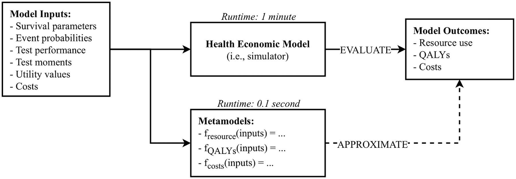
Illustration of how metamodels can be used in a health economic context to approximate the outcomes of the original health economic simulation model.

Figure 2, which will be discussed in detail throughout this article, includes an overview of how metamodels are developed. After identifying candidate metamodeling techniques, a set of experiments is to be generated. An experiment refers to a single sample of values of the model input parameters (thus, if there are k input parameters, a vector of length k), which is different from the use of the word experiment in the context of clinical studies. For health economic models, these input parameters may be probabilities, costs or utilities, for example. Next, the set of experiments is to be evaluated from the simulator to obtain a training data set that contains the experiments and their corresponding model outcomes, such as mean or incremental costs and quality-adjusted life-years (QALYs). Finally, metamodels are fitted to the training data set to approximate the relationship between simulator inputs and outcomes. Different metamodeling techniques can be used to approximate this relationship, each of which makes different assumptions about the functional form of the relationship between the inputs and outcomes of the simulator. Although the extent to which fitted metamodels can be interpreted varies, this is not of primary interest when using metamodels to reduce computational burden, because the main aim is to approximate simulators outcomes accurately and not to make inferences between inputs and outcomes. Most techniques approximate a single model-outcome, requiring multiple metamodels to approximate multiple simulator outputs. Hence, one metamodel can be used to approximate the net health benefit at a given willingness to pay, but 2 metamodels would be required to approximate costs and QALYs separately (Figure 1). After developing a metamodel, it needs to be validated by assessing its accuracy in approximating simulator outcomes, which is done based on a testing data set containing experiments and outcomes that should be similar but different from those included in the training data set.

Figure 2

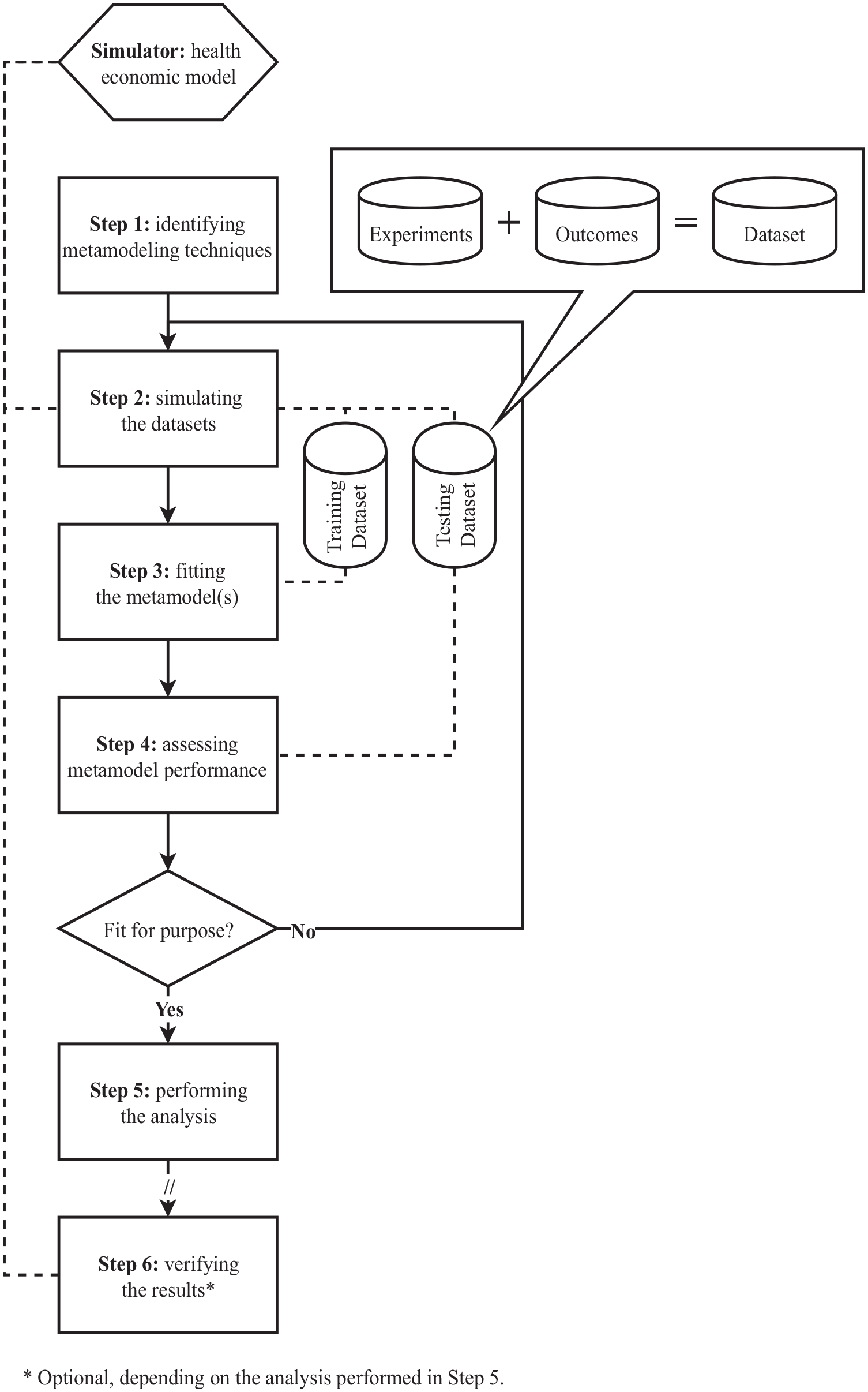
Process for developing, validating, and applying metamodeling methods in health economics.

Metamodeling methods are used widely across different fields of science and engineering, for example, to optimize designs of coronary stents,¹² high-speed trains,¹³ and groundwater remediation,¹⁴ as well as to estimate future water temperatures.¹⁵ In health economics, de Carvalho et al.¹⁶ recently demonstrated that a metamodel can be used to perform probabilistic analysis, which was not possible in a feasible time frame using their original model.¹⁶ A previous literature review identified only 13 additional applications of metamodeling methods in health economics, mostly aiming to perform value of information analysis and applying various, relatively basic metamodeling methods compared with those used in other fields of research, suggesting the field of metamodeling within health economics to be in its infancy.³ An important reason for the limited uptake of metamodeling methods within health economics may be that most health economic models and applied analyses have, until recently, been relatively simple and could often be performed within acceptable time frames. Other potential reasons include a lack of awareness of the potential of metamodeling methods to reduce runtime and a lack of guidance on how to apply these methods in a health economic context, which would explain the diversity in methods applied.

To increase awareness of the potential for applying metamodels within health economics, and to provide guidance for doing so, this study introduces the concepts of metamodeling to the wider health economic audience and presents a comprehensive, structured overview of metamodeling methods deemed suitable for use in a health economic context. Points of consideration for selecting and applying metamodeling methods are discussed, including directions specific to health economics.

Identification of Metamodeling Methods

Metamodeling methods (and the steps to be taken when applying them) were identified by a scoping literature search that was performed by K.D. This involved online searches, searches in Scopus and PubMed, and cross-referencing. Several publications that provide information on steps taken when applying metamodeling methods in health economics, identified in a recent review,³ were used as a starting point.^17-20 Method-specific information, other candidate metamodeling methods, and potentially relevant process steps were identified by iterative searches on methods and process steps introduced in these publications and by cross-referencing. For example, if the impact of different experimental designs on metamodel performance was discussed in an article found from a search on a specific metamodeling technique (i.e., structure of the metamodel), additional searches on these designs of experiments were performed to identify further information on these experimental designs and other designs of experiments. The iterative search process terminated when additionally found literature did not result in further inclusion of methods (i.e., until theoretical saturation was reached).

Metamodeling methods were included only if they are considered appropriate for use in health economics and have been commonly used in other fields of research, in line with the objective of the study. Methods were considered applicable to health economics if they are able to account for mixed (i.e., continuous and discrete) input parameters and continuous outcomes (i.e., response variables). Typical continuous input parameters of health economic models are, for example, costs and utilities, whereas the number of hospital days after a surgical intervention can be included as a discrete parameter. Similarly, typical continuous outcomes of interest are the net health or monetary benefit, total cost, and QALYs. Relevant steps to be taken when applying metamodeling methods in health economics were not prespecified but extracted from the literature as described above and structured in a process. Metamodeling methods and their characteristics were described according to this process and presented in a table or graphs when appropriate. In addition, examples of packages available to implement methods in R Statistical Software²¹ and Python²² were identified via an online search and introduced along with the corresponding methods. These 2 software environments were selected because they can be used to develop both the health economic simulation model and metamodel in a single script and are commonly used by academics, although other software environments such as SAS, Stata, and C++ can also be used to develop metamodels.

A Process for Metamodeling in Health Economics

A 6-step process for metamodeling in health economics was consolidated, covering methods from selecting suitable metamodeling techniques up to validating metamodel outputs against simulator outputs (Figure 2). A validated health economic simulation model (i.e., simulator) that is considered appropriate to perform the analysis of interest is a prerequisite, because although metamodels can theoretically be as accurate as their corresponding simulators, they cannot compensate for inaccuracies or bias in these simulators. Here, the analysis refers to what is to be analyzed using the original health economic model but is considered infeasible because of the associated computational burden. Depending on the analysis to be performed, the sixth step is facultative, as will be discussed. As for any type of modeling study, the process of metamodeling is iterative, since new insights may question prior decisions. Next, each process step will be described, including an overview of corresponding methods. An illustration of how this process would be applied to perform value of information analysis is presented in Appendix A.

Step 1: Identifying Candidate Metamodeling Techniques

Identification of theoretically suitable metamodeling techniques is based on study characteristics, including the analysis to be performed, type of input parameters (continuous, discrete, or mixed, i.e., both continuous and discrete), number of input parameters, and type of outcome (continuous or discrete). As discussed previously, the focus here is on techniques capable of handling mixed input parameters and continuous outcomes. In the presence of time or budget constraints for metamodel development, and when multiple techniques are considered appropriate for use, modelers can start by selecting and applying one of these techniques and only select and apply another technique if the resulting metamodel does not yield acceptable performance (see step 4).

Tappenden et al¹⁸ identified 5 metamodeling techniques for application in value of information analysis: linear regression, response surface methodology, multivariate adaptive regression splines, Gaussian processes, and neural networks. These techniques are complemented with symbolic regression, which was also identified from the review,¹⁹ and generalized additive models, which have been used previously for performing value of information analysis.^23,24 In Table 1, an overview of techniques and their characteristics is provided. For each metamodeling technique, this overview includes the typically required number of experiments (which we have defined as low: n < 500, or high: n ≥ 500), number of input parameters it allows (which we have defined as low: n < 20, or high: n ≥ 20), interpretability of the resulting metamodel structure (which we have classified as low: not or barely possible to understand relations between inputs and outputs, moderate: input-output relations can be understood to some extent, or high: input-output relations can be understood), and the description of any R and Python packages available to apply the technique. Regarding the interpretability of the metamodels’ structures, this is typically not of primary interest when using metamodeling for reducing computational burden, as accurate and fast approximation of simulator outcomes is the main goal.

Table 1

Overview of Candidate Metamodeling Techniques for Application in Health Economics, All of Which Are Able to Account for Mixed Input Parameters and Continuous Outcomes

Technique	Required Number of Experiments	Number of Inputs	Interpretability	R Package	Python Package	References
Response surface methodology	High	Large	Moderate	rsm ²⁵	sklearn ²⁶	10, 27, 28
Symbolic regression	High	Large	Moderate	RGP ^a,29	fastsr,³⁰ DEAP³¹	32, 33
Multivariate adaptive regression splines	High	Large	Low	Earth,³⁴ mda³⁵	py-earth ³⁶	10, 37, 38
Generalized additive models	High	Large	Low	gam,³⁹ mgcv,^40,41	pyGAM ⁴²	40, 43
Gaussian processes	Low	Low	Low	GPfit,⁴⁴ tgp^45,46	scikit-learn,⁴⁷ GPflow⁴⁸	10, 49
Neural networks	High	Large	Low	Neuralnet,⁵⁰ nnet⁵¹	keras,⁵² NeuPy⁵³	10, 38, 54

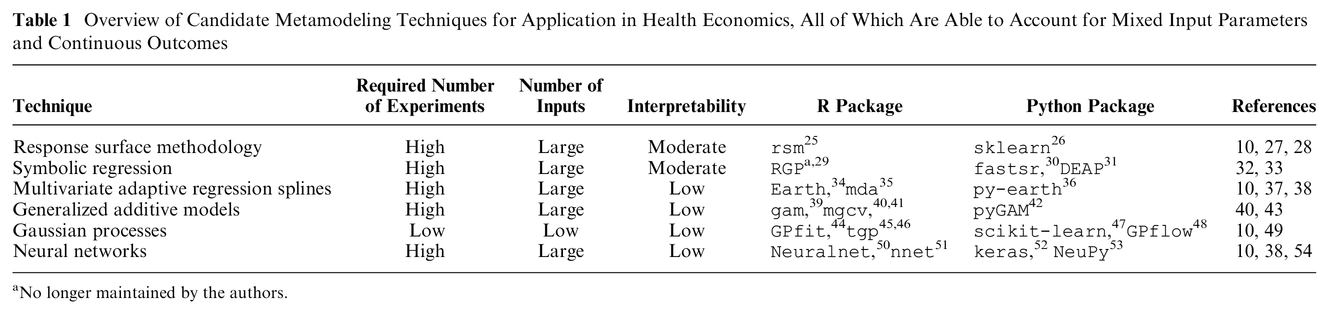
No longer maintained by the authors.

Simple linear regression is a statistical modeling technique well known in health economics and, theoretically, suitable for metamodeling. This assumes a linear relationship between independent variables (i.e., input parameters) and the dependent variable (i.e., outcome of interest) and is linear in the regression model parameters.⁵⁵ These models can easily be fitted to data sets of all sizes, including data sets with large numbers of experiments and input parameters, while allowing for both continuous and categorical input parameters. Although fitting linear regression models and interpreting their structure can be considered relatively easy, they are unlikely to be useful as metamodels of health economic simulation models, as the latter typically induce complex and nonlinear parameter interactions. More advanced techniques, allowing for more flexible model structures, are often better suited to represent such simulation models.

Response surface methodology is also linear in the regression model parameters but does not assume a linear input-output relationship, and it fits polynomial regression models to predict responses (i.e., outcomes).^10,27,28 Both continuous and categorical input parameters can be considered in response surface models, and data sets including large numbers of experiments and input parameters can be used. However, high nonlinearity will require higher-order polynomials, which will require larger numbers of experiments; hence, it will require larger up-front simulator runtime. Although polynomial models are more difficult to interpret compared with linear models, if desired, general trends of model parameter influence can still be extracted from their model structures.

Symbolic regression uses genetic programming to construct a mathematical expression from elementary operators (e.g., “+” and “×”) and elementary functions (e.g., “log”), accurately describing the relation between input parameters and the outcome of interest, without making any priori assumption about this relationship.^32,33 Fitting an accurate symbolic regression model may take substantial time, because of a potentially large number of candidate metamodels (i.e., large solution space). However, symbolic regression is capable of handling large data sets, including a large number of mixed input parameters. Symbolic regression models can be difficult to interpret unless the final expression is relatively simple or is simplified.

Multivariate adaptive regression splines were developed to model input-outcome relations that may not be constant across input space.^10,37,38,56 Regression spline modeling divides the outcome domain into intervals and then estimates an equation, typically a low-order polynomial, for each interval. Different types of splines can be distinguished, based on how the number of intervals and level of smoothness are defined. Fitting multivariate adaptive regression splines includes an automated input parameter importance analysis (see step 2). Although capable of handling large data sets of mixed input parameters, regression splines are prone to overfitting. In contrast to the previously discussed metamodeling techniques, the interpretability of multivariate adaptive regression splines is limited.

Generalized additive models assume that the dependent variable is a smooth, but unknown, function of the independent variables.^40,43 This unknown underlying smooth function is usually represented using splines, with the cubic spline as a common choice. In its simplest case, a univariate cubic spline represents an arbitrary smooth single-input function as a series of short cubic polynomials joined piecewise such that the function is twice differentiable at the “knots” (i.e., join points). The same spline can also be represented as the weighted sum of a series of predetermined “basis functions” that extend over the whole range of the function input. Simple univariate cubic splines have natural extensions to higher dimensions and to a metamodeling framework, in which the spline parameters (i.e., the basis function weights) are estimated from noisy data. Generalized additive models can handle large data sets and high numbers of input parameters, but their structure is difficult to interpret.

Gaussian process regression is a nonparametric regression method also known as Kriging.^10,49 Gaussian processes use information on neighbor experiments for new predictions while directly providing information on the uncertainty in these predictions. This is unique for metamodeling techniques, since other techniques require additional effort to obtain information on prediction uncertainty. Although Gaussian processes are capable of considering mixed input parameters,⁵⁷ Treed Gaussian processes have been developed specifically for this type of data.⁵⁸ The interpretability of Gaussian processes is low. A disadvantage of Gaussian processes is that computational burden, both in terms of fitting and predicting, increases dramatically with increasing numbers of experiments and parameters, limiting their applicability. Hence, Gaussian processes are often well suited for optimization problems, which are typically defined by limited numbers of decision parameters. Furthermore, input parameter importance analysis can be performed to reduce the number of parameters (see step 2) and, thereby, computational burden.

Neural networks are nonparametric models that are commonly found in machine learning applications. These models consist of networks of nodes (called neurons) and layers, which learn about relationships between inputs, either continuous or categorical, and outputs, typically using large data sets.^10,38,54 Although neural networks are commonly used for classification, they are also able to predict continuous outcomes.⁵⁹ Since no assumption regarding simulator structure is made, neural networks may well represent complex (i.e., nonlinear) health economic models. Developing large neural networks typically requires large numbers of experiments, which may pose challenges regarding obtaining sufficient simulator samples. Similar to multivariate adaptive regression splines, generalized additive models, and Gaussian processes, neural networks are “black boxes” that are hard to interpret.

In conclusion, as illustrated in the selection flowchart (Figure 3), Gaussian processes are particularly useful when obtaining sufficient simulator samples to apply the other techniques is infeasible. Response surface methodology, symbolic regression, multivariate adaptive regression splines, generalized additive models, and neural networks are typically useful when sufficient samples can be obtained from the simulator (i.e., original health economic model). If metamodel interpretation is important, response surface methodology and symbolic regression can be used to develop metamodels that may be interpretable to some extent.

Figure 3

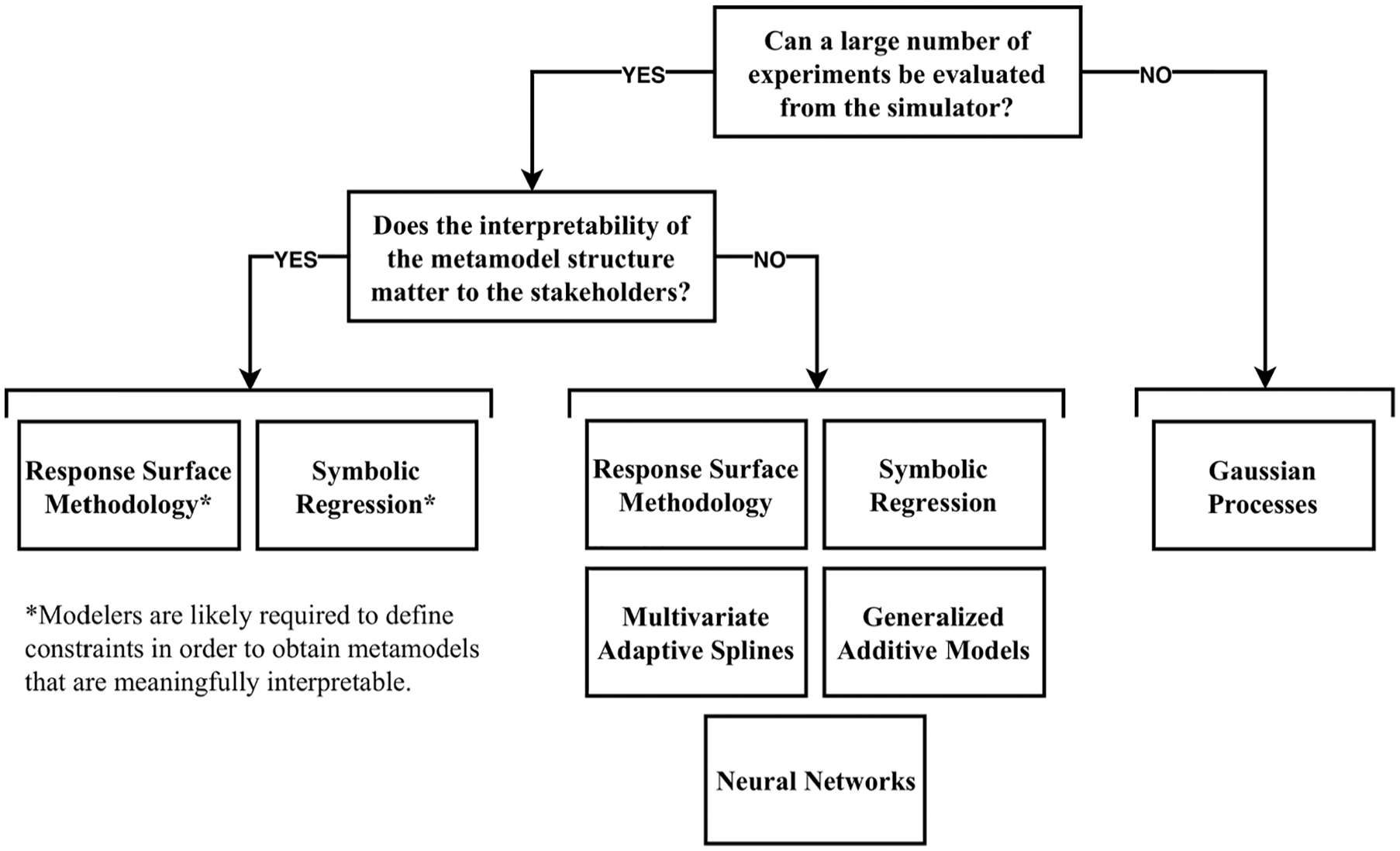
Flowchart for the selection of appropriate metamodeling techniques for a specific case study.

Step 2: Simulating Data Sets

Simulating data from the simulator is crucial in metamodeling studies, as metamodel performance is highly dependent on the data used for fitting.⁹ Modelers control the number and definition of experiments used for fitting metamodels, which is fundamentally different from prediction modeling studies, for which data are typically observed from clinical studies or registries.⁵⁵ Furthermore, challenges regarding handling missing data, reversed causality, omitted variables, and measurement error are not applicable to metamodeling. There are 5 key aspects to simulating data sets for metamodeling: 1) the number of data sets, 2) parameter ranges, 3) design of experiments, 4) number of experiments, and 5) analysis used for obtaining simulator outcomes. As explained previously, an experiment refers to the generation of a single sample of model input parameter values in a metamodeling context. Hence, the number of experiments does not refer to a number of (hypothetical) patients but to the number of sets of model input parameter values for which the simulation model is evaluated to create data sets for metamodel fitting and validation.

As in prediction modeling, 2 distinct data sets are preferred for metamodeling studies: one for fitting (i.e., training or development data set) and one for validation (i.e., testing or validation data set). In prediction modeling studies, validation data sets would typically be obtained by isolating a proportion of the data from a single cohort for internal validation or by gathering additional data from another “plausibly related” cohort for external validation.⁵⁵ In metamodeling, however, it is preferable to obtain 2 separate data sets from the simulator, each having a prespecified design with comprehensive coverage. Obtaining 1 large data set and separating it in 2 data sets for training and validation may compromise the coverage of these data sets: either data set may lack the structure and properties induced by the design of experiments used to generate the single large data set. By obtaining 2 separate data sets, their structure and properties according to the design of experiments used will be maintained, as will be discussed.

The range of values that is to be covered in the data sets requires careful consideration for each input parameter separately. Although metamodels are theoretically capable of extrapolating beyond the parameter ranges covered by the data set on which they were fitted, such extrapolations are not preferable. The ranges that need to be covered are determined by the ranges of interest in the analysis that is to be performed using the metamodel. For example, if a metamodel is developed to optimize a cancer screening strategy, the ranges that are considered feasible in the optimization should be the same as those in the data sets used for fitting and validating the used metamodel(s). If the screening interval in years is a parameter of interest and any value between 1 and 10 is considered feasible, the parameter range for this parameter in the training and testing data set should also range from 1 to 10.

Design of experiments methods determine how sets of samples of parameter values are selected, which are to be evaluated from the simulator in order to obtain data sets for fitting and validation.⁶⁰ The objective of these methods is to cover parameter spaces and parameter interactions as effectively and efficiently as possible (i.e., with the least number of experiments). Failing to represent the full parameter spaces and parameter interactions will decrease metamodel performance. Most common designs of experiments are so-called single-pass methods that first define a complete set of experiments, all of which are subsequently evaluated using the simulator.¹¹ Commonly used designs are random designs, full factorial designs, and Latin hypercube designs.

Random designs, also known as Monte Carlo sampling methods, obtain n sets of experiments by generating n draws from the joint probability distribution for the input parameters.⁶⁰ These designs require a large number of experiments to sufficiently cover the parameter space. Input distributions may be designed to cover a prespecified range with equal probability (i.e., uniform distributions) or may represent judgments about the true unknown value of some population quantity, for example, using Gamma distributions for parameters with a positive range.⁴ When a random design is used, 1 large data set can be separated in 2 data sets for fitting and validation, while maintaining its random properties.

Full factorial designs fully enumerate possible combinations of discrete parameter values.¹¹ More specifically, for n values of k parameters, a full factorial design represents all n^k combinations of these parameter values. Although full factorial designs are able to cover the full parameter space and interactions, the number of experiments increases exponentially with the number of parameters, and they are, therefore, often infeasible to use. Fractional factorial designs have been introduced to address challenges regarding high numbers of experiments when using factorial designs and consist of subsets of full factorial designs.⁶¹

Latin hypercube designs have been used often for designing computer experiments, as they efficiently cover the full parameter space.^60,62,63 In its simplest form, Latin hypercube samples represent random combinations of values for each parameter, which are equally spaced between their minimum and maximum value for each parameter. More often, Latin hypercube samples represent random combinations of random values from equally sized bins that cover the parameters’ domains. Over the years, more advanced versions have been developed, such as the maximin Latin hypercube design,⁶⁴ which maximizes the minimum distance between design points, and orthogonal Latin hypercube designs.⁶⁵

Figure 4 illustrates how random, full factorial, and maximin Latin hypercube designs may define 9 experiments for 2 continuous parameters TestCost and ConsultationCost. Although simulators and metamodels in practice will have more than 2 parameters, this figure clearly demonstrates differences between the designs. It shows that parameter spaces are most effectively covered by maximin Latin hypercube sampling, as the corresponding experiments are properly distributed over all bins of the parameter ranges. Conversely, the full factorial design covers some bins multiple times and others not at all. The randomly sampled experiments also cover some bins multiple times and others not at all, although which bins those are is determined by chance. From this figure, it can also be seen why simply isolating a proportion of experiments from the data set for model validation is not appropriate, and a separate data set needs to be simulated when a nonrandom design is used. Isolating a (random) proportion from a data set generated according to a full factorial or Latin hypercube design will result in a training data set that no longer covers the full parameter space consistently. The remaining experiments will no longer cover all bins of the parameter domain in a Latin hypercube design or all parameter value combinations in a full factorial design.

Figure 4

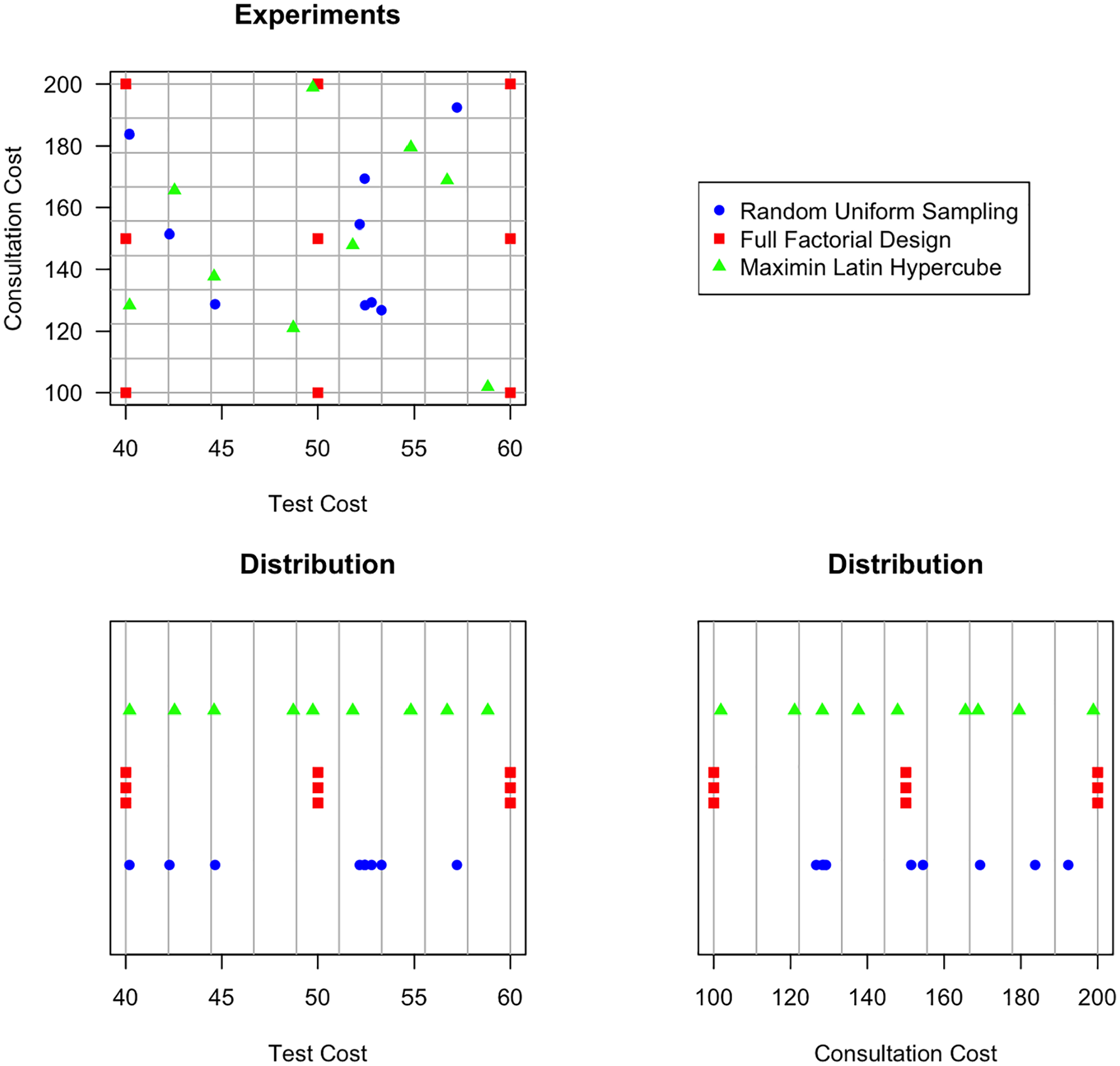
Illustration of how a random uniform sample, full factorial design, and maximin Latin hypercube sample may define 9 experiments for 2 continuous parameters, TestCost and ConsultationCost.

In general, Latin hypercube designs are preferable for both training and testing data sets, especially when only a limited number of experiments can be evaluated from the simulator in the available time. Optimized Latin hypercube designs can easily be generated in most software environments, for example, using the lhs package in R⁶⁶ or the pyDOE package in Python. However, these designs are challenging to apply when constraints on combinations of parameters are applicable. Although some work has been done on conditioned Latin hypercube designs, accounting for inequality constraints,⁶⁷ this might not enable all constraints to be accounted for. In such situations, factorial designs can be used if the resulting number of experiments is considered feasible. However, when using factorial designs for continuous variables, a finite set of discrete values within the continuous parameter range needs to be defined, which may result in an infeasible number of experiments to cover those parameters’ ranges at the desired level of detail. If using a factorial design is considered infeasible, random designs allow constraints to be accounted for easily. However, random designs are likely less efficient, which may result in suboptimal solution space coverage and, consequently, lower metamodel performance, especially when a limited number of experiments can be evaluated from the simulator.

How many experiments are required (i.e., how large the n should be) heavily depends on the desired metamodel accuracy, which will be discussed in step 4. In addition, the design of experiments method used and how well the metamodeling techniques match the unknown relation between inputs and outputs influence the number of experiments required.^68,69 A general rule of thumb is to start with n = 10 × k, where k refers to the number of input parameters.^69,70 After evaluating model performance for the initial set of experiments (see step 4), n may be increased until the desired level of overall accuracy is achieved (see Appendix A for an example). Alternatively, adaptive sampling methods may be applied to improve accuracy in local regions of the parameter space,⁵¹ but these methods are outside the scope of this study (see the Discussion section). If the desired model accuracy cannot be achieved with a feasible number of experiments, importance analysis methods may be applied to reduce the number of input parameters k, by analyzing which parameters are most important in terms of predicting the simulator outcomes.^18,72,73 Including only the most parameters might result in less complex metamodel structures, and if redundant input parameters can be removed, metamodel accuracy may improve as overfitting is reduced.

Whether a deterministic or probabilistic analysis needs to be performed to evaluate experiments from the simulator depends on the analysis to be performed with the metamodel. In a deterministic analysis, the simulator is evaluated once for the expected values of the input parameters.⁴ In a probabilistic analysis, the simulator is evaluated numerous times, typically thousands of times, based on parameter values sampled from distributions that reflect the uncertainty in the parameter values (i.e., second-order uncertainty). If a model is nonlinear, which most health economic models are, health economic outcomes from a deterministic analysis are not equal to those of a probabilistic analysis.⁷⁴ If metamodels are being used to perform model probabilistic analysis or value of information, simulator outcomes based on a deterministic analysis should be used. If the aim is to perform calibration or optimization, simulator outcomes based on probabilistic analyses are preferred, because these are the values expected to be observed in reality given the current information. However, performing a probabilistic analysis for each experiment might not be feasible because of the required simulator runtime. In that case, outcomes from a deterministic analysis may be used to approximate the outcomes of a probabilistic analysis, although this should be clearly noted as a limitation when reporting the results.

The stability of outcome estimates is another important aspect. If stochastic uncertainty, also referred to as uncertainty on the patient level or first-order uncertainty, is reflected in a patient-level simulation model, sufficient hypothetical patients need to be simulated to obtain stable outcomes. Similarly, regardless of whether first-order uncertainty is reflected, sufficient probabilistic analysis runs need to be performed to obtain stable point estimates. When insufficient hypothetical patients are simulated, or probabilistic analysis runs performed, the subsequent noise in the data used for fitting metamodels may have a pernicious effect on metamodel performance. Outcomes can be considered stable if the outcomes obtained from simulations with different random numbers, but with the same input parameter values, are sufficiently similar. What defines “sufficiently similar” differs among case studies and should be discussed with all relevant stakeholders (e.g., care providers, decision makers, and modelers). Obtaining stable outcomes may require a substantial number of patients to be simulated or simulation runs to be performed and may not be feasible in practice. However, to reduce the number of patients to be simulated or the number of runs to be performed to obtain stable outcomes, variance reduction techniques may be applied, such as using common random numbers when comparing strategies.^75,76

Step 3: Fitting Metamodels

After evaluating an initial set of experiments from the simulator, this training data set can be used to fit selected metamodeling techniques. Steps involved in the fitting processes differ between techniques as well as any settings to be provided. We refer to the corresponding literature and software documentation to learn about the steps to be taken and settings to be provided (see step 1 and Table 1). As a basic example, some metamodeling techniques or software packages require input parameters to be rescaled. Fitting metamodels is an iterative process, in which settings may be adapted, or more experiments may be evaluated from the simulator, after assessing model performance (see step 4).

Step 4: Assessing Metamodel Performance

Assessing the performance of fitted metamodels is essential to further improve that performance, by iteratively improving (extending) the design of the training data set used or adapting the settings for fitting these models. In addition, an initially selected metamodeling technique may be deemed inappropriate if performance does not reach an acceptable level, resulting in exclusion of this technique from the list of potential candidates (step 1). Performance can be assessed using the testing data set evaluated from the simulator in step 2. Since metamodels of health economics models will typically predict continuous scale outcomes, of main interest is to quantify how close predictions are to actual simulator outcomes. Assessing accuracy and comparing different metamodels can be done graphically and using quantitative performance criteria. A validation plot, with predicted values on the x-axis and observed values from the simulator on the y-axis, is fundamental in assessing model performance and presents information on systematic trends as well as general performance (see Appendix A for an example). Several quantitative performance criteria are available, including mean or maximum values of the absolute error, absolute relative error, and squared error, all of which may be normalized using the sample range or standard deviation, and summarized by their mean or maximum values, and R².^38,69,77,78

It is important to be aware of performance criteria characteristics when selecting one, or several, to compare metamodels or to assess whether model performance is acceptable. For example, compared with mean absolute errors, mean squared errors place more weight on outliers. In addition, compared with squared errors, setting a desired level of accuracy is more straightforward for absolute (relative) errors, as these can be set by answering questions such as, “What is the maximum mean deviation in predicted life-years the metamodel is allowed to have compared with the simulator outcomes?” The performance that can be considered acceptable for deciding to apply a metamodel for performing analyses differs among case studies and should be based on input from all stakeholders. For example, when the point estimate for the incremental QALYs is 0.18 QALYs, an absolute error of 0.01 QALY may be considered appropriate by stakeholders. Since different performance criteria and definitions of acceptable performance may yield alternative conclusions, these should be decided upon prior to metamodel development.

Step 5: Applying the Metamodel

Once a metamodel has been developed and validated, it can be used to perform analyses that could not be performed in a feasible time period with the original health economic model. Previous applications of metamodels in health economics include value of information analysis, model calibration, optimization, probabilistic analysis, and obtaining stable outcomes over multiple runs with the same input values.³ In addition, metamodels can be used in online tools for which limited computer resources are available. For example, see de Carvalho et al.¹⁶ for a demonstration of metamodels used for probabilistic analysis or Appendix A for an illustration of the presented 6-step process for performing value of information analysis. Another example may be to use metamodels for evaluating a large set of (thousands of) screening strategies, for example, to identify the starting age, screening interval, and number of screening rounds that optimize health and economic outcomes.

Step 6: Verifying Results (Optional)

If metamodels are used for optimization purposes, it is recommended to reevaluate a certain number of best strategies identified by the metamodel using the original health economic model, to assess whether their outcome and ordering meaningfully differ. By providing these results, decision makers are better informed about the expected impact of choosing a good but not optimal candidate strategy for implementation, which may be favored over the optimal strategy for practical reasons. For other types of analyses, such as probabilistic or value of information analysis, additional verification will not add to the validation of step 4, because reevaluating a number of strategies using the simulator will yield approximately the same error values as those obtained in step 4. Although this will also be the case for several best-performing strategies when optimization is performed, knowing the true outcomes and ordering of the strategies according the simulator is informative, whereas knowing the true outcome for a specific probabilistic analysis run is not of any value.

Discussion

This study provides an introduction to metamodeling methods that can be used to reduce the computational burden of advanced analyses with health economic models and addresses challenges regarding the selection and application of these methods. Similar to ordinary statistical regression modeling, different methods, which are discussed, are available with their own advantages, disadvantages, and underlying assumptions, and directions for selecting and implementing these methods are provided. Selected methods are structured in a comprehensive 6-step process that can be followed to ensure essential modeling steps are covered, as it includes all relevant design choices. In addition, the process discussed can be used as a structure to effectively and efficiently communicate metamodeling studies, to increase modeling transparency and reproducibility.

Given that tools and packages are available to generate experiments according to specific designs and to fit different types of metamodels, for example, in R and Python, applying metamodeling methods is feasible for health economic analysts. Currently available software and results from this study enable analysts to perform computationally demanding analyses with their models, such as value of information analysis, model calibration, and optimization. The benefits of developing metamodels are relevant to analyses using patient-level simulation methods, such as microsimulation state-transition modeling and discrete event simulation, but also to cohort models used to perform analyses that require a large number of model evaluations.

Applying metamodeling methods can reduce computational burden, but this usually comes at the price of introducing additional uncertainty in the model outputs. Consequently, checking whether underlying assumptions are met and checking metamodel performance are crucial to success and essential to build confidence in the metamodel. Since modelers typically have access to the original health economic model, validation of the metamodel is often not a problem, although it is likely to be more demanding in terms of effort compared with developing the metamodel itself. The starting point for building any metamodel, however, should be a realistic and validated health economic model, since metamodels can theoretically be as accurate as their corresponding simulators but will not compensate for inaccuracies in these simulators. Moreover, when metamodels are used for optimization, the strategies considered, and possibly identified as optimal, may not be supported by (the data underlying) the simulator. Caution is required when such extrapolation is (automatically) performed, and such optimization results should serve only to initiate discussion on the appropriateness and validity of the simulator and the data supporting it. In addition, the application of metamodeling methods requires communication of metamodeling design choices made in publications, for which space is typically already limited. Hence, metamodeling studies may be published separately from their simulator to ensure the metamodeling process can be appropriately described. Furthermore, there is a “sweet spot” for metamodeling: sufficient experiments need to be evaluated using the simulator to develop an accurate metamodel, but evaluating all experiments of interest should not be feasible.

Several technical challenges remain regarding the application of metamodeling methods in health economics. Simulators in health economics may include complex behavior, such as rigid cutoffs due to clinical decision rules, which may be complex for metamodeling techniques to capture. In addition, (combinations of) model input parameters may be subject to constraints, which are difficult to incorporate in efficient designs of experiments, such as Latin hypercube sampling. If sufficient samples can be evaluated from the simulator to use random or full factorial designs in which constraints can be accounted for more easily, however, this might not be an issue. Alternatively, more advanced adaptive sampling strategies may need to be applied.

Not all metamodeling methods are directly suitable for application in health economics and hence have not been discussed. However, it is important to note that some techniques, such as those that can be used for categorical outcomes (i.e., classification), could theoretically be applied in health economics after discretizing continuous outcomes. Such an approach has been taken previously by using a binary outcome to reflect whether one treatment was preferred over another in a logistic regression model.⁷³ Similarly, examples of packages for R and Python were discussed, whereas additional packages are likely to be available and other software environments can also be used to develop metamodels, such as Stata, SAS, and C++. In addition, alternative performance criteria for metamodel validation can be found, or may be developed, based on study-specific needs. With regard to sampling methods, only single-pass methods have been discussed, whereas iterative methods, also known as adaptive sampling or active learning methods, also exist.^79,80 Iterative methods use an initial data set for fitting an initial metamodel, which is subsequently used in an iterative process to identify additional experiments to be added to the data set, to update the initial metamodel, and to check the updated metamodel performance, until this performance is in accordance with a predefined threshold.⁷¹ The additional experiments are sampled in the area in which performance needs to be improved. Although iterative methods are more efficient compared with single-pass methods, they are substantially more complicated to implement and require simulators to be available in the same software environment used for generating experiments and fitting the metamodel. Nevertheless, these methods may be useful if insufficient experiments according to a single-pass design can be obtained to develop an accurate metamodel. Also, alternative designs of experiments are available, such as D-optimal designs, which are efficient and can account for constraints, but for which an linear or quadratic model simulator model structure should be known,⁸¹ or for so-called Sobol sequences, which may be more efficient compared with Latin hypercube designs with low-dimension (i.e., number of input parameters) problems.^82,83

Future metamodeling applications should further illustrate the potential and use of these research methods and also identify common challenges. Once the field of metamodeling in health economics has evolved, good research practices (i.e., consensus guidance) can be identified to further improve the quality of metamodeling studies.

Supplemental Material

appendix.rjf_online_supp – Supplemental material for Introduction to Metamodeling for Reducing Computational Burden of Advanced Analyses with Health Economic Models: A Structured Overview of Metamodeling Methods in a 6-Step Application Process

Supplemental material, appendix.rjf_online_supp for Introduction to Metamodeling for Reducing Computational Burden of Advanced Analyses with Health Economic Models: A Structured Overview of Metamodeling Methods in a 6-Step Application Process by Koen Degeling, Maarten J. IJzerman, Mariel S. Lavieri, Mark Strong and Hendrik Koffijberg in Medical Decision Making

Footnotes

The authors declared no potential conflicts of interest with respect to the research, authorship, and/or publication of this article.

The authors received no financial support for the research, authorship, and/or publication of this article.

ORCID iD

Koen Degeling

Supplemental Material

Supplementary material for this article is available on the Medical Decision Making Web site at .

References

Brennan

Chick

Davies

A taxonomy of model structures for economic evaluation of health technologies. Health Econ. 2006;15(12):1295–310.

Karnon

Haji

Ali

Afzali

When to use discrete event simulation (DES) for the economic evaluation of health technologies? A review and critique of the costs and benefits of DES. Pharmacoeconomics. 2014;32(6):547–58.

Degeling

IJzerman

Koffijberg

A scoping review of meta-modeling applications and opportunities for advanced health economic analyses. Exp Rev Pharmacoecon Outcomes Res. 2018;19(2):1–7.

Briggs

Weinstein

Fenwick

EAL

Karnon

Sculpher

Paltiel

AD.

Model parameter estimation and uncertainty analysis: a report of the ISPOR-SMDM Modeling Good Research Practices Task Force Working Group–6. Med Decis Making. 2012;32(5):722–32.

Heath

Manolopoulou

Baio

A review of methods for analysis of the expected value of information. Med Decis Making. 2017;37(7):747–58.

Crown

Buyukkaramikli

Thokala

, et al. Constrained optimization methods in health services research—an introduction: report 1 of the ISPOR Optimization Methods Emerging Good Practices Task Force. Value Health. 2017;20(3):310–9.

Karnon

Stahl

Brennan

Caro

Mar

Möller

Modeling using discrete event simulation: a report of the ISPOR-SMDM Modeling Good Research Practices Task Force–4. Med Decis Making. 2012;32(5):701–11.

Law

AM.

Simulation Modeling and Analysis. Singapore: McGraw-Hill Higher Education; 2007.

Sacks

Welch

Mitchell

Wynn

HP.

Design and analysis of computer experiments. Stat Sci. 1989;4(4):409–23.

10.

Barton

RR.

Simulation metamodels. In: Proceedings of the 1998 Winter Simulation Conference. Washington, DC: IEEE Computer Society; 1998:167–76.

11.

Simpson

Poplinski

Koch

Allen

JK.

Metamodels for computer-based engineering design: survey and recommendations. Eng Comput. 2001;17(2):129–50.

12.

Wang

, et al. Multi-objective optimization of coronary stent using Kriging surrogate model. Biomed Eng Online. 2016;15(2):148.

13.

Liang

Yao

Chen

Multi-objective aerodynamic optimization of the streamlined shape of high-speed trains based on the Kriging model. PloS One. 2017;12(1):e0170803.

14.

Ouyang

Lin

Deng

Cheng

Conservative strategy-based ensemble surrogate model for optimal groundwater remediation design at DNAPLs-contaminated sites. J Contam Hydrol. 2017;203:1–8.

15.

Butcher

Schmidt

Johnson

Nover

Clark

CM.

Estimating future temperature maxima in lakes across the United States using a surrogate modeling approach. PloS One. 2017;12(11):e0183499.

16.

de Carvalho

Heijnsdijk

EAM

Coffeng

de Koning

HJ.

Evaluating parameter uncertainty in a simulation model of cancer using emulators. Med Decis Making. 2019;39(4):405–13.

17.

Rojnik

Naversnik

Gaussian process meta-modeling in Bayesian value of information analysis: a case of the complex health economic model for breast cancer screening. Value Health. 2008;11(2):240–50.

18.

Tappenden

Chilcott

Eggington

Oakley

McCabe

Methods for expected value of information analysis in complex health economic models: developments on the health economics of interferon-beta and glatiramer acetate for multiple sclerosis. Health Technol Assess. 2004;8(27):1–78.

19.

Willem

Stijven

Vladislavleva

Broeckhove

Beutels

Hens

Active learning to understand infectious disease models and improve policy making. PLoS Comput Biol. 2014;10(4):e1003563.

20.

Yousefi

Ferreira

RPM

Kim

Fogliatto

FS.

Chaotic genetic algorithm and Adaboost ensemble meta-modeling approach for optimum resource planning in emergency departments. Artif Intell Med. 2018;84:23–33.

21.

R Core Team. R: A Language and Environment for Statistical Computing. R Foundation for Statistical Computing; 2018 Available from: https://www.r-project.org/. Accessed December 5, 2018.

22.

Python Core Team. Python: A Dynamic, Open Source Programming Language. Python Software Foundation; 2019. Available from: https://www.python.org/. Accessed July 25, 2019.

23.

Strong

Oakley

Brennan

Estimating multiparameter partial expected value of perfect information from a probabilistic sensitivity analysis sample: a nonparametric regression approach. Med Decis Making. 2014;34(3):311–26.

24.

Strong

Oakley

Brennan

Breeze

Estimating the expected value of sample information using the probabilistic sensitivity analysis sample: a fast, nonparametric regression-based method. Med Decis Making. 2015;35(5):570–583.

25.

Lenth

RV.

Response-surface methods in R, using rsm. J Stat Softw. 2009;32(7):1–17.

26.

Pedregosa

Varoquaux

Gramfort

, et al. Scikit-learn: machine learning in Python. J Machine Learn Res. 2011;12:2825–2830.

27.

Carson

Maria

Simulation optimization: methods and applications. In: Proceedings of the 1997 Winter Simulation Conference. Atlanta, (GA): IEEE Computer Society; 1997:118–26.

28.

Myers

Montgomery

Anderson-Cook

CM.

Response Surface Methodology: Process and Product Optimization Using Designed Experiments. Hoboken, NJ: Wiley; 2016.

29.

Flasch

Mersmann

Bartz-Beielstein

Stork

Zaefferer

rgp: R genetic programming framework. 2014. Available from: https://cran.r-project.org/src/contrib/Archive/rgp/Accessed December 5, 2018.

30.

Fusting

fastsr: fast symbolic regression powered by genetic programming. 2017. Available from: https://pypi.org/project/fastsr/. Accessed July 25, 2019.

31.

Fortin

F-A

De Rainville

F-M

Gardner

M-A

Parizeau

Gagné

DEAP: evolutionary algorithms made easy. J Machine Learn Res.2012;13:2171–5.

32.

Gaucel

Keijzer

Lutton

Tonda

Learning Dynamical Systems Using Standard Symbolic Regression. Berlin: Springer Berlin Heidelberg; 2014.

33.

Koza

JR.

Genetic Programming: On the Programming of Computers by Means of Natural Selection. Cambridge, MA: MIT Press; 1992.

34.

Milborrow

earth: multivariate adaptive regression splines. 2017. Available from: https://CRAN.R-project.org/package=earth. Accessed December 5, 2018.

35.

Hastie

Tibshirani

mda: mixture and flexible discriminant analysis. 2017. Available from: https://CRAN.R-project.org/package=mda. Accessed December 5, 2018.

36.

Rudy

A Python implementation of Jerome Friedman’s multivariate adaptive regression splines. 2013. Available from: http://contrib.scikit-learn.org/py-earth/. Accessed July 25, 2019.

37.

Knafl

Ding

Adaptive Regression for Modeling Nonlinear Relationships. Basel, Switzerland: Springer International; 2016.

38.

Xie

Goh

TN.

A systematic comparison of meta-modeling techniques for simulation optimization in decision support systems. Appl Soft Comput. 2010;10(4):1257–73.

39.

Hastie

gam: generalized additive models. 2018. Available from: https://CRAN.R-project.org/package=gam. Accessed December 5, 2018.

40.

Wood

Generalized Additive Models: An Introduction with R. Boca Ralton. London: Taylor & Francis; 2006.

41.

Wood

mgcv: mixed GAM computation vehicle with automatic smoothness estimation. 2018. Available from: https://cran.r-project.org/web/packages/mgcv/mgcv.pdf. Accessed December 5, 2018.

42.

Servén

Brummitt

pyGAM: generalized additive models in Python. 2018. Zenodo. doi:10.5281/zenodo.1208723

43.

Hastie

Tibshirani

Generalized additive models. Stat Sci. 1986;1(3):297–310.

44.

MacDonald

Ranjan

Chipman

{GPfit}: an {R} package for fitting a Gaussian process model to deterministic simulator outputs. J Stat Softw. 2015;64(12):1–23.

45.

Gramacy

RB.

tgp: an R package for Bayesian nonstationary, semiparametric nonlinear regression and design by Treed Gaussian process models. J Stat Softw. 2007;19(9):1–46.

46.

Gramacy

Taddy

Categorical inputs, sensitivity analysis, optimization and importance tempering with tgp version 2, an R package for Treed Gaussian process models. J Stat Softw. 2010;33(6):1–48.

47.

Pedregosa

Varoquaux

Gramfort

, et al. Scikit-learn: machine learning in Python. J Machine Learn Res. 2011;12:2825–30.

48.

Matthews

van der Wilk

Nickson

, et al. GPflow: a Gaussian process library using TensorFlow. J Machine Learn Res. 2017;18(40):1–6.

49.

O’Hagan

Kingman

JFC

. Curve fitting and optimal design for prediction. J R Stat Soc Ser B (Methodol). 1978;40(1):1–42.

50.

Fritsch

Guenther

neuralnet: training of neural networks. 2016. Available from: https://CRAN.R-project.org/package=neuralnet. Accessed December 5, 2018.

51.

Venables

Ripley

BD.

Modern Applied Statistics with S. New York: Springer; 2002.

52.

Chollet

, et al. Keras. 2015. Available from: https://keras.io. Accessed July 25, 2019.

53.

Shevchuk

NeuPy: neural networks in Python. 2019. Available from: http://neupy.com/pages/home.html. Accessed July 25, 2019.

54.

Dreyfus

Neural Networks: Methodology and Applications. Berlin: Springer Berlin Heidelberg; 2005.

55.

Steyerberg

EW.

Clinical Prediction Models: A Practical Approach to Development, Validation, and Updating. New York, NY: Springer; 2009.

56.

Madan

Ades

Price

, et al. Strategies for efficient computation of the expected value of partial perfect information. Med Decis Making. 2014;34(3):327–42.

57.

Swiler

Hough

Qian

Storlie

Lee

Surrogate Models for Mixed Discrete-Continuous Variables. Cham, Vietnam: Springer International.

58.

Gramacy

Lee

HKH

. Bayesian Treed Gaussian process models with an application to computer modeling. J Am Stat Assoc. 2008;103(483):1119–30.

59.

Hurrion

RD.

Using a neural network to enhance the decision making quality of a visual interactive simulation model. J Oper Res Soc. 1992;43(4):333–41.

60.

Garud

Karimi

Kraft

Design of computer experiments: a review. Comput Chem Eng. 2017;106:71—95.

61.

Box GEP. Statistics for Experimenters: Design, Innovation, and Discovery. Hoboken, NJ: Wiley; 2005.

62.

Husslage

BGM

Rennen

van Dam

den Hertog

. Space-filling Latin hypercube designs for computer experiments. Optimization and Engineering. 2011;12(4):611–30.

63.

McKay

Beckman

Conover

WJ.

A comparison of three methods for selecting values of input variables in the analysis of output from a computer code. Technometrics. 1979;21(2):239–45.

64.

Johnson

Moore

Ylvisaker

Minimax and maximin distance designs. Journal of Statistical Planning and Inference. 1990;26(2):131–48.

65.

KQ.

Orthogonal column latin hypercubes and their application in computer experiments. J Am Stat Assoc. 1998;93(444):1430–9.

66.

Carnell

lhs: Latin gypercube samples. 2018. Available from: https://CRAN.R-project.org/package=lhs. Accessed December 5, 2018.

67.

Petelet

Iooss

Asserin

Loredo

Latin hypercube sampling with inequality constraints. AStA Adv Stat Anal. 2010;94(4):325–39.

68.

Levy

Steinberg

DM.

Computer experiments: a review. AStA Adv Stat Anal. 2010;94(4):311–24.

69.

Loeppky

Sacks

Welch

WJ.

Choosing the sample size of a computer experiment: a practical guide. Technometrics. 2009;51(4):366–76.

70.

Jones

Schonlau

Welch

WJ.

Efficient global optimization of expensive black-box functions. Journal of Global Optimization. 1998;13(4):455–92.

71.

Crombecq

Laermans

Dhaene

Efficient space-filling and non-collapsing sequential design strategies for simulation-based modeling. Eur J Oper Res. 2011;214(3):683–96.

72.

Jalal

Dowd

Sainfort

Kuntz

KM.

Linear regression meta-modeling as a tool to summarize and present simulation model results. Med Decis Making. 2013;33(7):880–90.

73.

Merz

Small

Fischbeck

PS.

Measuring decision sensitivity: a combined Monte Carlo-logistic regression approach. Med Decis Making. 1992;12(3):189–96.

74.

Briggs

Claxton

Sculpher

MJ.

Decision Modelling for Health Economic Evaluation. Oxford, UK: Oxford University Press; 2006.

75.

Kahn

Marshall

AW.

Methods of reducing sample size in monte carlo computations. J Oper Res Soc Am. 1953;1(5):263–78.

76.

Murphy

Klein

Smolen

Klein

Roberts

SD.

Using common random numbers in health care cost-effectiveness simulation modeling. Health Serv Res. 2013;48(4):1508–25.

77.

Gano

Kim

Brown

Comparison of three surrogate modeling techniques: datascape, kriging, and second order regression. Presented at: 11th AIAA/ISSMO Multidisciplinary Analysis and Optimization Conference, American Institute of Aeronautics and Astronautics, Portsmouth, VA, 2006.

78.

Kleijnen

JPC

Sargent

A methodology for fitting and validating metamodels in simulation. Eur J Oper Res. 2000;120(1):14–29.59.

79.

Alison

Sahinidis

Miller

DC.

Learning surrogate models for simulation-based optimization. AIChE J. 2014;60(6):2211–27.

80.

Wilson

Sahinidis

NV.

The ALAMO approach to machine learning. Comput Chem Eng. 2017;106:785–95.

81.

de Aguiar

Bourguignon

Khots

Massart

Phan-Than-Luu

D-optimal designs. Chemometrics and Intelligent Laboratory Systems. 1995;30(2):199–210.

82.

Kucherenko

Albrecht

Saltelli

Exploring multi-dimensional spaces: a comparison of Latin hypercube and quasi Monte Carlo sampling techniques. 2015. Available from: https://arxiv.org/abs/1505.02350. Accessed June 20, 2018.

83.

Soboĺ

IM.

Quasi-Monte Carlo methods. Prog Nucl Energy. 1990;24(1):55–61.

Supplementary Material

Please find the following supplemental material available below.

For Open Access articles published under a Creative Commons License, all supplemental material carries the same license as the article it is associated with.

For non-Open Access articles published, all supplemental material carries a non-exclusive license, and permission requests for re-use of supplemental material or any part of supplemental material shall be sent directly to the copyright owner as specified in the copyright notice associated with the article.

0.00 MB

0.10 MB