Sage Journals: Discover world-class research

Abstract

Background. When data on preferences are not available, analysts rely on condition-specific or generic measures of health status like the SF-12 for predicting or mapping preferences. Such prediction is challenging because of the characteristics of preference data, which are bounded, have multiple modes, and have a large proportion of observations clustered at values of 1. Methods. We developed a finite mixture model for cross-sectional data that maps the SF-12 to the EQ-5D-3L preference index. Our model characterizes the observed EQ-5D-3L index as a mixture of 3 distributions: a degenerate distribution with mass at values indicating perfect health and 2 censored (Tobit) normal distributions. Using estimation and validation samples derived from the Medical Expenditure Panel Survey 2000 dataset, we compared the prediction performance of these mixture models to that of 2 previously proposed methods: ordinary least squares regression (OLS) and two-part models. Results. Finite mixture models in which predictions are based on classification outperform two-part models and OLS regression based on mean absolute error, with substantial improvement for samples with fewer respondents in good health. The potential for misclassification is reflected on larger root mean square errors. Moreover, mixture models underperform around the center of the observed distribution. Conclusions. Finite mixtures offer a flexible modeling approach that can take into account idiosyncratic characteristics of the distribution of preferences. The use of mixture models allows researchers to obtain estimates of health utilities when only summary scores from the SF-12 and a limited number of demographic characteristics are available. Mixture models are particularly useful when the target sample does not have a large proportion of individuals in good health.

Keywords

EQ-5D SF-12 prediction mapping mixture models Tobit health-related quality of life

Quality-adjusted life-years (QALYs), calculated by combining life-years gained with a measure of preferences over health states into a single composite measure that captures both mortality and morbidity, are commonly used to quantify benefit in economic evaluations.¹ To obtain societal preferences (or health utilities) from questionnaires, a patient survey instrument measuring general health status is scored using country-specific weights derived from large-scale valuation studies that reflect preferences over health states.^2,3 After the patient survey is scored, the resulting metric is often referred to as a “preference index,” from which QALYs can be calculated.

A widely used instrument for measuring preferences is the EQ-5D, which currently has preference-scoring algorithms for many countries, including the US.⁴ The EQ-5D is a standardized measure of health status developed to provide a simple, generic measure of health for clinical and economic appraisal, consisting of 5 questions.⁵ In the EQ-5D-3L version, each question has 3 levels of severity, while a newer version (EQ-5D-5L) has 5 levels.⁶ Together, the 5 questions or domains are meant to capture a holistic view of health.⁷ In the UK, the National Institute for Health and Care Excellence (NICE) has indicated that the EQ-5D is the preferred measure of health-related quality of life (HRQL) in adults.⁸ In the US, the Institute of Medicine (IOM) recommended the direct elicitation of preferences or the use of generic preference indexes like those derived from the EQ-5D.⁹

Unfortunately, the EQ-5D or other preference-based instruments are not routinely collected in clinical trials or existing secondary data sources, thereby limiting their value for economic evaluation.¹⁰ This problem has prompted researchers to propose several methods for predicting (or “mapping”) the EQ-5D based on other instruments that measure health functioning. In the US, these efforts gained steam after the release of the 2000 Medical Expenditure Panel Survey (MEPS), a nationally representative sample of the US noninstitutionalized population. The 2000 MEPS started asking a large and representative sample of respondents to complete both the EQ-5D-3L and the Short-Form Health Survey (SF-12), an instrument that measures general health status.¹¹ The SF-12 is widely available in clinical trials and in some secondary data sources. The NICE has indicated that when the EQ-5D instrument is not available, prediction methods can be used to obtain a predicted preference index from other instruments that measure HRQL.¹²

The unusual distribution of the EQ-5D-3L, however, makes it challenging to predict. The index is bounded on the right at 1, representing preferences for “perfect health,” and it can also take negative values, indicating preference for health states considered “worse than death.”² In addition, the EQ-5D-3L distribution tends to have 3 distinct modes, and in samples representing the general population, a large proportion of responses are clustered at 1. To date, most of the methods used to predict the EQ-5D-3L index from the SF-12 instrument in a representative sample of the US population have ignored some or all of these characteristics, with the consequence that prediction may be systematically biased.¹³ While statistical methods such as ordinary least squares (OLS), Tobit regression, and two-part models have been previously proposed, none fully captures the idiosyncratic characteristics commonly observed in societal preferences.

The objective of this article is to develop and implement a statistical model that takes into account all the characteristics of the EQ-5D-3L index and to investigate under which circumstances our proposed model leads to improved prediction in a US sample compared with other alternatives proposed in the literature. Our model assumes that the observed EQ-5D-3L index is a mixture of 3 distributions: a degenerate distribution with mass at preference values indicating perfect health and 2 censored normal (Tobit) distributions, which take into account the bounded nature of the EQ-5D-3L index. We use the mental and physical components of the SF-12 health survey as predictors, along with a limited number of covariates. We compare predictions from our finite mixture models to the best-performing alternatives proposed in the literature: linear regression and two-part models.¹³

Background

EQ-5D-3L

The EQ-5D-3L questionnaire is made of 2 components: a descriptive classification component and a Visual Analogue Scale (VAS). The EQ-5D-3L descriptive component consists of 5 domains of health: mobility, self-care, usual activities, pain and discomfort, and anxiety/depression. Each question has 3 possible answers that capture a respondent's ability to perform each of the 5 domains: no problems, some or moderate problems, and extreme problems or unable to perform the activity. The EQ-5D-3L describes a total of 3⁵ (i.e., 243) possible response patterns, each defining a “health state.” Perfect health is defined as having no problem in any of the 5 domains, while the worst possible state is being unable to perform any of the 5 activities. To transform the EQ-5D-3L descriptive system into a measure that represents preferences, each of the health states defined by the descriptive system is converted to a preference index using algorithms derived from valuation studies. In the US, the valuation study sample represented the civilian noninstitutionalized population.²

Figure 1 shows the distribution of the EQ-5D-3L preference index using the MEPS 2000 data (described below) for selected age groups and medical conditions. Several characteristics of the distribution are worth nothing. First, a large proportion of individuals (43.65%) have an EQ-5D-3L index of 1 (Panel A), indicating preferences for perfect health. The proportion of individuals in perfect health decreases with age, as shown in Panels B to E, and for those individuals who have a self-reported medical condition, Panels F to I. Second, the distribution exhibits 3 modes, at approximately 0.17, 0.75, and 1 (Panel A). The location of the modes differs according to the characteristics of the sample, particularly the number and severity of comorbid conditions. Finally, the range of possible EQ-5D scores is limited. The lowest possible score is –0.594 and the highest is 1.

Figure 1

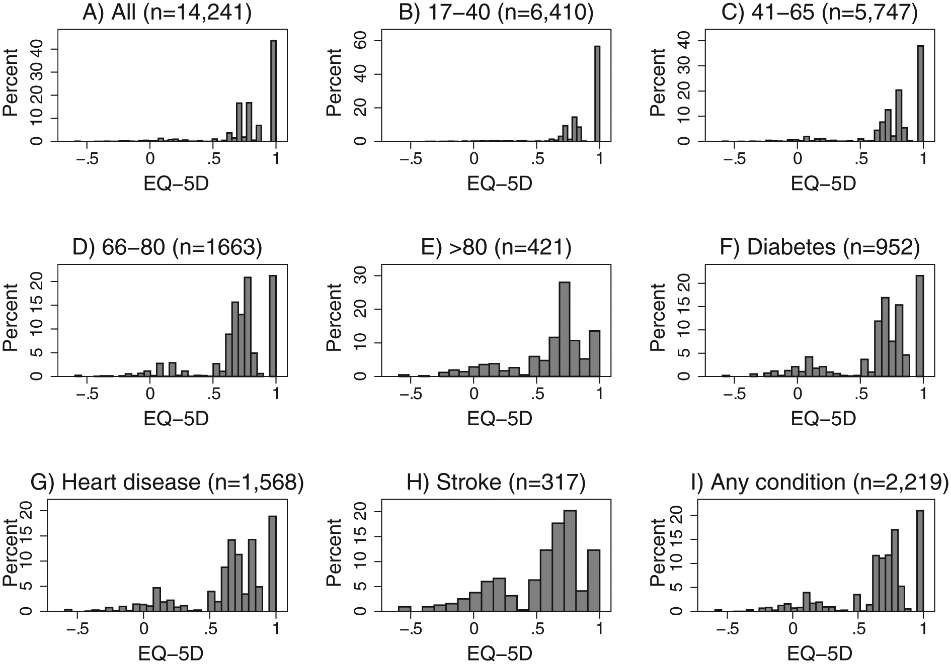
Distribution of EQ-5D-3L by age group and medical condition. Data source: MEPS, 2000. All sample (A); by age group (B–E), and for selected self-reported conditions (F–I). “Any condition” refers to those who have heart disease, stroke, and/or diabetes. Some individuals have more than 1 condition.

SF-12

The 12-item Short-Form Health Survey (SF-12) is an instrument derived from the longer 36-item Short-Form (SF-36),¹¹ which was designed to measure general health functioning. The SF-12 items measure physical or emotional limitations, physical functioning, pain, general health, vitality, social functioning, and mental health problems. It provides 2 summary scores, the Physical Component Summary (PCS) and the Mental Component Summary (MCS). Scores are standardized; the mean score in the population is 50 with a standard deviation of 10 points. Higher scores indicate better functioning in each domain. The SF-12 instrument is not routinely used in economic evaluations because the resulting functioning scales are not expressed in terms of preferences, although algorithms have been developed for that purpose.^14–16

Previous Prediction Approaches

Several methods have been proposed for predicting the EQ-5D-3L from the SF-12 components using MEPS data. These methods can be divided into 2 types, depending on whether the prediction target is the EQ-5D-3L preference index itself or the responses to the EQ-5D-3L descriptive system.

One of the earliest approaches using MEPS data focused on the prediction of the mean EQ-5D-3L preference index using mean values of the PCS and MCS from the SF-12.¹⁷ Franks and others¹⁸ used individual-level data instead and OLS regression with SF-12 components as predictors. They found that OLS models explained approximately 63% of the total variance and performed well for EQ-5D-3L scores close to the observed mean, but they cautioned that their models performed poorly for the worse health states. In addition, OLS models underpredict scores of those in perfect health as these models do not take into account the upper bound of the EQ-5D-3L preference index. Recognizing that the EQ-5D-3L index is bounded at 1, Sullivan and Ghushchyan¹⁹ compared OLS models to Tobit regression and censored least absolute deviations (CLAD) models and concluded that the OLS model outperformed Tobit models, but the investigators recommended CLAD models when the only predictors available are mental and physical scores of the SF-12. Another way to account for the large proportion of EQ-5D-3L scores clustered at 1 is with two-part models, which are commonly used to model cost data.²⁰ Li and Fu²¹ suggested that two-part models are a superior alternative to Tobit and CLAD models for predicting EQ-5D-3L scores, although those authors did not directly compare two-part models with OLS or Tobit/CLAD models using MEPS data.

Gray and others²² used a different approach. They used multinomial models to first estimate the probability that a respondent would select a particular level of response to each question in the EQ-5D-3L (modeling each of the EQ-5D questions separately). These estimated probabilities were then used to create a simulated pattern of responses, which were then scored and translated into the preference index. The advantage of this method is that if the predicted response pattern is accurate, the predicted EQ-5D-3L index will preserve the characteristics of the observed EQ-5D-3L index. However, Chuang and Kind¹³ compared this approach with OLS, CLAD, and two-part models using MEPS data and concluded that OLS was the best method for predicting the EQ-5D-3L, although the accuracy of OLS deteriorated in less healthy groups.

Numerous research articles describe methods for predicting preference-based measures from non-preference-based instruments using datasets from the US and other countries, as well as using instruments other than the SF-12 as predictors. Brazier and others²³ conducted a review of 30 studies and found that most of them used OLS models, with approximately half using either the EQ-5D-3L preference index or the descriptive system as an outcome. The investigators concluded that the performance of models in terms of goodness-of-fit and prediction was variable and difficult to generalize given the myriad of methods and instruments used. Other research has focused on simulation studies comparing different methods that could be potentially used to model preference-based outcomes like the EQ-5D-3L, including mixture models. In simulation studies, Pullenayegum and others²⁴ compared latent class models (mixture of 2 normals) to OLS, Tobit, CLAD, and two-part models and recommended the use of OLS models with robust standard errors. In contrast, two-part models were recommended by Huang and others²⁵ over alternatives that included latent class models assuming normal densities. Both studies were concerned about modeling bounded data and did not explore other mixture models. Hernandez and others²⁶ considered a longitudinal mixed-effects mixture of censored normals, which they called “adjusted limited dependent variable mixture models” (ALDVMMs), using a disability measure, the Health Assessment Questionnaire–Disability Index (HAQ-DI), and a pain measure as predictors of the EQ-5D-3L, in a randomized trial of patients with rheumatoid arthritis. Longworth and others²⁷ compared several mapping methods, including two-part models, Tobit models, multinomial models, and ALDVMMs using cancer-specific HRQL measures as predictors in a sample of patients with different types of cancer and disease stages.

Our methodological approach is similar to that of Hernandez and others,²⁶ but we focus on predicting the EQ-5D using a broader measure of health (SF-12) in a nationally representative sample of the US population, incorporating widely available covariates in a cross-sectional context.

Methods

Data

The MEPS is a nationally representative survey of the noninstitutionalized US population. The survey collects detailed information on respondents’ demographics, health care utilization and expenditures, self-reported medical conditions, insurance coverage, and socioeconomic status. In the year 2000, the MEPS added a self-administered module asking a subset of respondents to complete both the EQ-5D and the SF-12 questionnaires.^17,28,29

Models

Traditional parametric regression models assume that the observed outcome is a realization from some probability distribution. For example, linear regression assumes that the outcome of interest distributes normally with unknown variance and mean given by a linear combination of covariates. In contrast, finite mixture models assume that the outcome comes from a combination of 2 or more distributions, which are mixed with unknown probabilities. The objective is to simultaneously estimate the parameters of each distribution and the mixture probabilities.

Formally, finite mixture models assume that the probability density generating the observed outcome is a convex combination of k different densities:

f (y) = \sum_{j = 1}^{k} π_{j} f_{j} (y | x, θ_{j}),

where 0 ≤ $π_{j}$ ≤ 1 and $\sum_{j = 1}^{k} π_{j} = 1$ . Here, $θ_{j}$ is a vector of parameters describing the density distribution f_j, $π_{j}$ is a mixture probability, and x is a vector of covariates. The $π_{j}$ values are unknown parameters to be estimated along with the parameters $θ_{j}$ . Mixture models can be extended by allowing the mixture probabilities to be a function of a vector of covariates z with parameters $α : π_{j} (z' α_{j})$ , where covariates z may be different from those in x . Each density describes a “class” or “component,” and the number of components k must be specified a priori. The densities can be discrete or continuous and of different types. For instance, a well-known example of a finite mixture model is the zero inflated Poisson (ZIP) model,³⁰ typically used to model count data with excess zeroes. The ZIP model is a mixture of 2 different distributions: a Poisson distribution and a degenerate distribution with mass at zero. Since the Poisson distribution has support at zero, observed zeroes may come from either of the 2 components.

Finite mixture models can also be used to classify observations into distinctive classes. The posterior probability that an observation belongs to class c is given by

\Pr (y \in class c | x, y, \hat{θ}) = \frac{{\hat{π}}_{c} f_{c} (y | x, {\hat{θ}}_{c})}{\sum_{j = 1}^{c} {\hat{π}}_{j} f_{j} (y | x, {\hat{θ}}_{jc})},

where ${\hat{π}}_{j}$ and ${\hat{θ}}_{j}$ are the estimated parameters of the mixture given in Equation 1. In general, an observation is assigned to the class with the greatest posterior probability.³¹Equation 2 is used when the outcome y is observed and the objective is to assign an observation to 1 of the classes or components.

Our application of finite mixture models assumes that the EQ-5D-3L preference index is a mixture of 3 classes: a degenerate distribution and 2 censored normal distributions, also known as a Tobit model. With the aim of modeling expenditure data on durable goods, Tobin introduced the concept of censored normals in the econometrics literature.^32,33 Expenditure on durable goods can only take positive values, and because households do not purchase durable goods on a regular basis, a sizable portion of expenditures over a period of time are zero. A censored normal model assumes that the observed outcome comes from a latent random variable that follows a normal distribution but realizations of the random variable are censored if they cross a threshold value. In the case of expenditure data, the threshold value is zero, and realizations of the latent variable that are less than zero are observed to be zero.

Formally, the Tobit model assumes that the latent variable $y^{*}$ distributes normally with mean $x' β$ and unknown variance $σ^{2}$ . That is,

y^{*} = x' β + ε,

where $ε ~ N (0, σ^{2})$ . The observed outcome $y$ is defined as $y = y^{*}$ if $y^{*} > L$ and $y = L$ if $y^{*} \leq L$ . In the expenditure data example, $L = 0$ , and therefore the observed outcome is zero when the latent variable is negative and $N (x' β, σ^{2})$ when the latent variable is greater than zero.^34,35

The density for the standard Tobit model is given by

f (y) dy = {[\frac{1}{σ} \emptyset (\frac{y - x' β}{σ}) dy]}^{(1 - d)} {[Φ (- \frac{x' β}{σ})]}^{d},

where $\emptyset (\cdot)$ is the standard normal density, $Φ (\cdot)$ is the standard cumulative normal distribution function, and d is an indicator variable equal to 1 if $y = 0$ and zero otherwise. The second bracket in Equation 3 is simply the probability that the latent variable is less than zero. The expected value conditional on observed covariates for an observation randomly drawn from the population, which could be censored, is given by

E [y | x] = Φ (\frac{x' β}{σ}) (x' β + σ \frac{\emptyset (x' β / σ)}{Φ (x' β / σ)}) .

The density of our proposed mixture model consists of 2 Tobit censored normal components and a degenerate distribution with mass at zero. This density is an extension of Equation 3 and is given by the expression

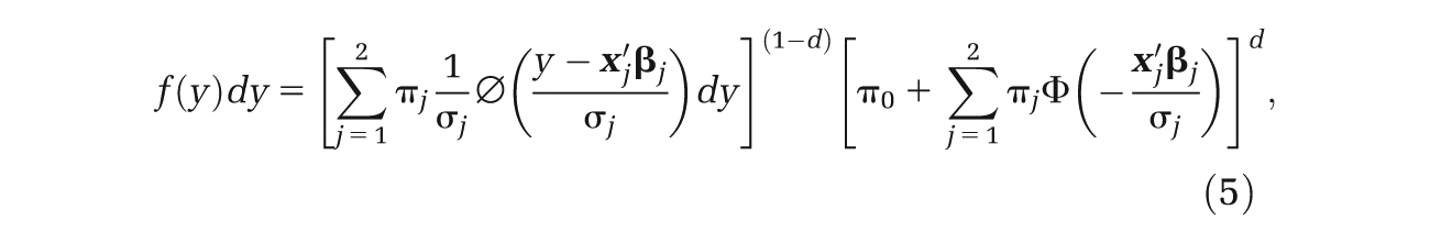
f (y) dy = {[\sum_{j = 1}^{2} π_{j} \frac{1}{σ_{j}} \emptyset (\frac{y - x_{j}^{'} β_{j}}{σ_{j}}) dy]}^{(1 - d)} {[π_{0} + \sum_{j = 1}^{2} π_{j} Φ (- \frac{x_{j}^{'} β_{j}}{σ_{j}})]}^{d},

where π_j are the mixture probabilities. Here, $π_{0} = (1 - π_{1} - π_{2})$ is the mixture probability of the degenerate component. To model the EQ-5D-3L preference index using the density given by Equation 5, we define y = 1 – EQ-5D-3L. That is, we model the reversed EQ-5D-3L preference index.³⁶ The choice of scale does not affect prediction or the statistical properties of the model, but care must be taken when interpreting the sign of the estimated set of coefficients $β_{j}$ as they represent marginal changes on the reversed scale. In the sections below, we present results on the original EQ-5D-3L scale.

The model described by Equation 5 can be extended by making the mixture probabilities to be functions of covariates using a multinomial transformation:

π_{j} = \frac{\exp (z' α_{j})}{1 + \exp (z' α_{1}) + \exp (z' α_{2}),}

where $α_{0} = 0$ . The vector of covariates z models the probability that an observation belongs to a class or component, while the vector of covariates x models how covariates affect the mean of the components.

Assuming independent observations following the density described by Equations 5 and 6, we estimated the parameters by maximum likelihood. For this purpose, we developed a Stata program that maximizes the log-likelihood.³⁷ In general, the likelihood function of a mixture model is difficult to maximize because of the possibility of multiple local maxima and nonconcave regions.³¹ We developed an algorithm to choose appropriate starting values, which we tested extensively via simulations. We ensured our models converged to a global maximum by trying different sets of feasible starting values. Details of the Stata command and the strategy for choosing starting values are given in Appendix A.

Two types of predictions can be calculated from our models. For models with constant mixture probabilities, the predicted EQ-5D-3L is the sum of the predictions from each component weighted by their estimated mixture probabilities ${\hat{π}}_{j}$ . For the Tobit components, predictions are calculated following Equation 4. We call this type of prediction “weighted average” (WA) predictions. For models in which mixture probabilities are conditional on covariates z , individuals can be first assigned to a class based on the maximum of the estimated mixture probabilities ${\hat{π}}_{j} (z {\hat{α}}_{j})$ . The predicted EQ-5D-3L is then the prediction corresponding to the assigned class. We call this type of prediction a “conditional on estimated class” (CEC) prediction.

Analyses

We randomly divided MEPS 2000 data into estimation and validation samples of roughly equal size and estimated 4 types of models using the estimation sample: 1) mixture models without covariates in the mixing probabilities, 2) mixture models with covariates in the mixing probabilities, 3) OLS regression, and 4) two-part models, in which the first part estimates the probability that the EQ-5D index is less than 1 using a logistic model, and the second part uses an OLS model to estimate the expected EQ-5D score based only on those with observed EQ-5D < 1. Assuming that the parts in the two-part model are independent, the predicted EQ-5D index is the product of the predicted probabilities from the first part and the predicted expected value from the second part.²⁰

Although the MEPS dataset has a rich set of covariates, in practical applications using other datasets, analysts will likely have access to only a limited set of demographic variables. To examine the performance of our method in such circumstances, we only used age, sex, and education in addition to PCS and MCS as predictors. For each method, we selected the best-fitting model specification identified by the Bayesian information criterion (BIC). Functional forms considered included quadratic terms and interactions. In some models, we included the sum of the mental and physical components rather than both components. To facilitate the interpretation of interactions and the intercept, continuous variables were centered. Age was centered at 65, and PCS and MCS were centered at their mean value of 50, with the sum centered at 100. Education was entered as an indicator variable equal to 0 if the respondent did not complete high school and 1 otherwise.

After selecting the best model for each method, we compared their prediction performance using the root mean square error (RMSE) and the mean absolute error (MAE). Both RMSE and MAE quantify the discrepancy between observed and predicted values, but in RMSE larger errors have greater influence than smaller errors.

We conducted a series of sensitivity analyses to evaluate the performance of our model under various circumstances. Because the shape of the distribution varies with age and health status, we compared the prediction performance using a subsample of individuals with diabetes, stroke, or heart disease (Figure 1, Panel I). To determine the performance of our model at the tails of the distribution, we categorized the EQ-5D-3L index into 4 levels (<0, 0–0.699, 0.7–0.899, 0.9–1) and compared the prediction performance by level.

Results

There were a total of 14,241 observations in the MEPS 2000 with complete data in all covariates. Table 1 shows the characteristics of the estimation and validation samples by age, sex, race, education, and selected self-reported comorbidities. In the combined sample, the mean EQ-5D-3L was 0.81 (s = 0.24). The mean MCS was 51.12 (s = 9.49), and the mean PCS was 48.90 (s = 10.34). Mean EQ-5D-3L and PCS scores declined with age and were lower for those subjects with comorbid conditions. The lowest average EQ-5D-3L, PCS, and MCS scores corresponded to medical conditions that are highly debilitating: stroke and emphysema. For the combined sample, the Pearson correlation between the EQ-5D-3L index and the PCS and MCS scores was 0.68 and 0.48, respectively.

Table 1

Baseline Characteristics by Sample

	Estimation Sample (n = 7120)				Validation Sample (n = 7121)
	%	$\bar{X}$ (s)			%	$\bar{X}$ (s)
	%	EQ-5D-3L	PCS	MCS	%	EQ-5D-3L	PCS	MCS
Age, years
18–40	45.53	0.88 (0.18)	52.54 (7.10)	51.31 (8.96)	44.49	0.86 (0.20)	52.29 (7.49)	50.95 (9.30)
41–65	39.87	0.79 (0.25)	48.03 (10.59)	51.12 (9.57)	40.48	0.79 (0.25)	48.29 (10.37)	50.92 (9.56)
66–80	11.33	0.71 (0.27)	41.40 (12.10)	51.83 (10.16)	12.02	0.71 (0.26)	41.42 (11.86)	51.40 (9.95)
>80	3.26	0.60 (0.33)	35.60 (11.60)	50.70 (11.11)	2.65	0.61 (0.29)	34.73 (11.60)	49.88 (11.46)
$\bar{X}$ (s)	44.79 (17.4)				44.91 (17.20)
Sex
Male	46.21	0.83 (0.23)	49.86 (9.74)	52.34 (8.68)	46.22	0.84 (0.22)	49.69 (9.85)	52.09 (8.81)
Female	53.79	0.80 (0.25)	48.12 (10.80)	50.36 (9.92)	53.78	0.79 (0.25)	48.18 (10.67)	49.99 (1.03)
Race
White	83.08	0.81 (0.24)	48.96 (10.33)	51.31 (9.40)	83.68	0.84 (0.24)	48.90 (10.34)	50.98 (9.52)
Black	13.65	0.80 (0.26)	48.33 (10.60)	51.09 (9.55)	12.89	0.80 (0.26)	48.48 (10.35)	50.98 (9.76)
Other	3.27	0.84 (0.23)	50.49 (9.59)	51.20 (9.38)	3.43	0.83 (0.24)	49.81 (9.81)	50.41 (9.45)
Education
Less than HS	56.78	0.78 (0.26)	47.43 (11.00)	50.68 (9.95)	57.03	0.78 (0.26)	47.44 (11.03)	50.25 (10.06)
HS or more	43.22	0.86 (0.20)	50.89 (9.08)	52.06 (8.61)	42.97	0.85 (0.19)	50.79 (8.95)	51.90 (8.72)
Asthma	8.46	0.73 (0.28)	45.37 (12.07)	49.20 (10.84)	8.76	0.72 (0.30)	45.26 (12.22)	48.42 (11.19)
Current smoker	21.94	0.78 (0.26)	48.39 (10.52)	49.54 (10.28)	22.67	0.78 (0.26)	48.29 (10.70)	49.09 (10.61)
Diabetes	6.63	0.65 (0.33)	40.20 (12.57)	48.31 (11.14)	6.74	0.67 (0.31)	40.54 (12.09)	48.84 (10.75)
Emphysema	1.38	0.53 (0.32)	31.69 (11.01)	45.74 (12.30)	1.43	0.61 (0.30)	33.83 (11.53)	47.27 (11.99)
Heart disease	9.44	0.63 (0.33)	38.75 (13.11)	48.48 (11.12)	10.05	0.66 (0.31)	39.64 (12.48)	48.91 (11.34)
Hypertension	22.78	0.70 (0.29)	42.55 (12.30)	49.90 (10.62)	23.58	0.72 (0.28)	43.21 (11.79)	49.79 (1.54)
Joint pain	30.9	0.68 (0.29)	43.93 (12.33)	49.41 (10.77)	32.4	0.69 (0.28)	43.36 (12.05)	49.17 (10.65)
Stroke	2.02	0.53 (0.36)	35.18 (12.09)	46.35 (11.93)	2.43	0.57 (0.34)	35.17 (11.52)	47.85 (12.38)

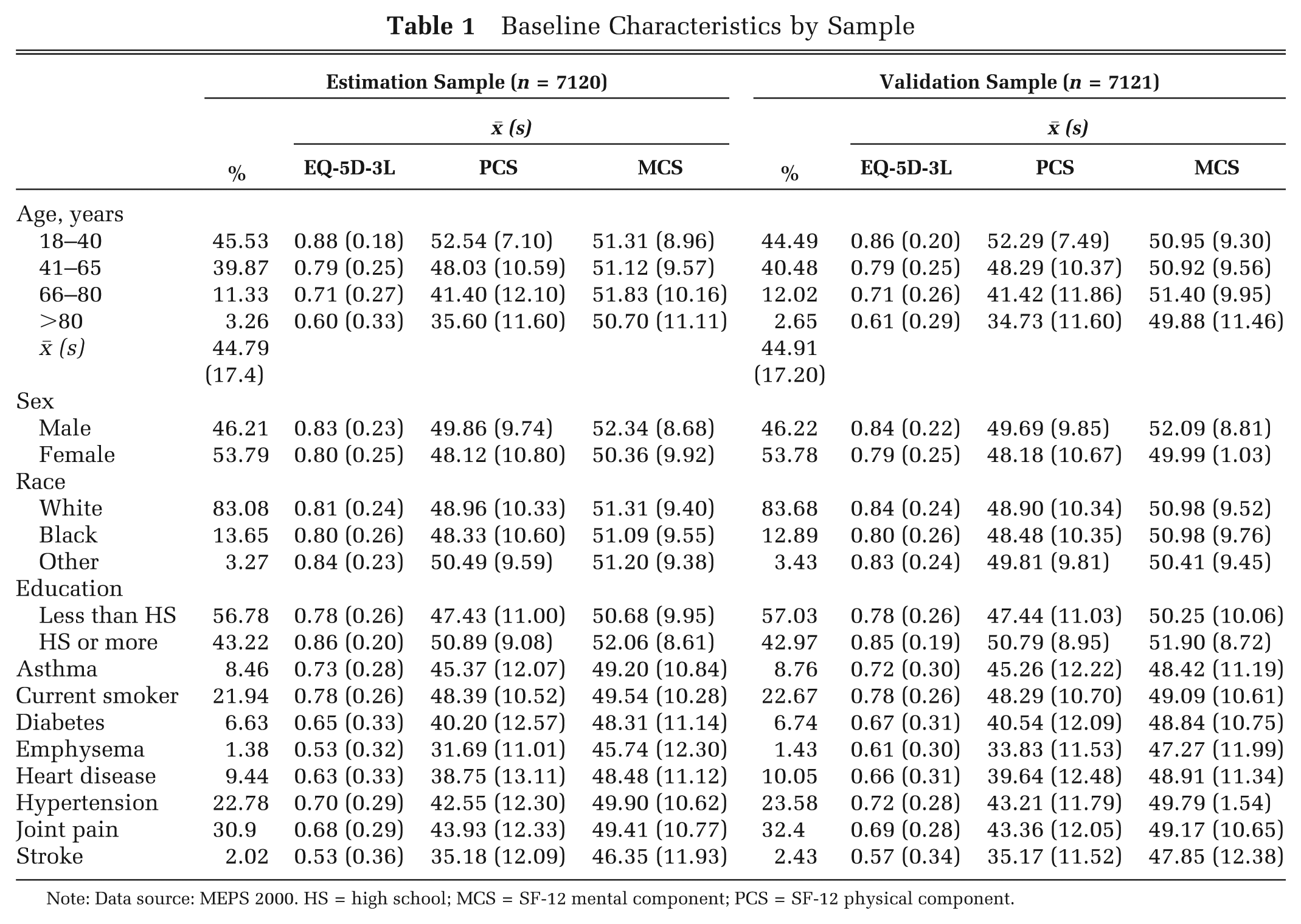
Note: Data source: MEPS 2000. HS = high school; MCS = SF-12 mental component; PCS = SF-12 physical component.

Using the BIC, the best-fitting model within each method had different functional forms. Table 2 shows the estimated coefficients for each model and method. The Mixture 1 model is a model with constant mixture probabilities. The best model of this type corresponds to a mixture of 2 Tobit models, with the degenerate distribution having zero estimated mixture probability. The Mixture 2 model, which allows covariates to alter the mixture probabilities, is considerably simpler. In this model, the mean EQ-5D-3L in each class is a function only of PCS and MCS, and the probability of class membership is a function of PCS, MCS, and age. The estimated average predicted mixture probability corresponding to the degenerate distribution is 0.43, which is similar to the observed proportion of observations with an EQ-5D-3L of 1.

Table 2

Model Parameters by Method

Variable	OLS	Two-Part Model		Mixture 1				Mixture 2
Variable	OLS	First Part	Second Part	Class 1	Pr1	Class 2	Pr2	Class 1	Pr1	Class 2	Pr2
					0.6328*		0.3671*
					(0.0070)		(0.0071)
Age	−0.0023	0.2368***	−0.0056*	−0.192**		−0.0058***			0.0264***		0.0212***
Age	(0.0021)	(0.0437)	(0.0025)	(0.0072)		(0.0011)			(0.0021)		(0.0040)
Age²	0.002***	−0.0241*	0.0001	0.0052**		0.0002
Age²	(0.0005)	(0.0107)	(0.0007)	(0.0021)		(0.0003)
Male	−0.005	−0.0295	−0.0094	−0.008		−0.0013
Male	(0.0036)	(0.0633)	(0.0052)	(0.0153)		(0.0020)
HS or more	0.016***	−0.2655***	0.0172*	0.0522**		0.0078***
HS or more	(0.0037)	(0.0642)	(0.0054)	(0.0159)		(0.0020)
PCS	0.0115***							0.0046***	−0.2152***	0.0096***	−0.3208***
PCS	(0.0003)							(0.0001)	(0.0073)	(0.0006)	(0.0091)
PCS²	−0.0001***
PCS²	(0.0001)
MCS	0.0085***							0.002***	−0.1414***	0.0046***	−0.2491***
MCS	(0.0002)							(0.0001)	(0.0053)	(0.0006)	(0.0074)
PCS²	−0.0001***
PCS²	(0.0001)
PCS + MCS		−0.1661***	0.0044***	0.0359***		0.0028***
PCS + MCS		(0.0044)	(0.0003)	(0.0011)		(0.0001)
(PCS + MCS)²		−0.0018***	−0.0002***	0.0003***		−0.0001***
(PCS + MCS)²		(0.0003)	(0.0001)	(0.0001)		(0.00001)
Intercept	0.8172***	1.9158***	0.7476***	0.9908***		0.7521***		0.7692***	1.5638	0.3351***	−1.955***
Intercept	(0.0043)	(0.0807)	(0.0052)	(0.0176)		(0.0022)		(0.0010)	(0.0678)	(0.0160)	(0.1439)

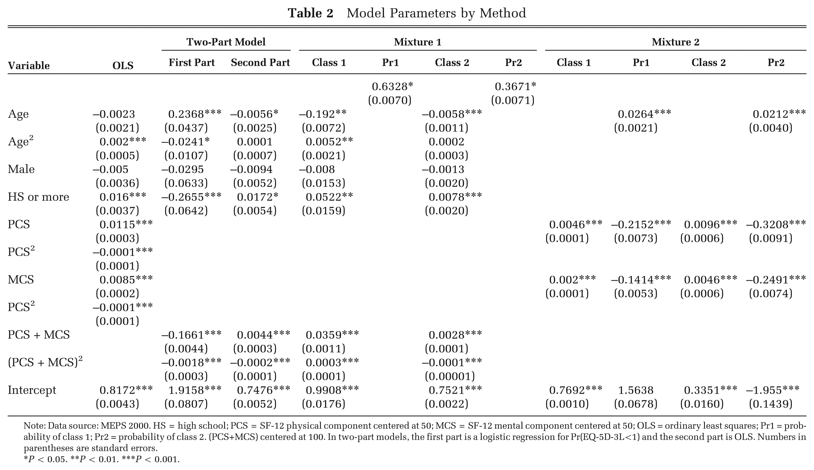
Note: Data source: MEPS 2000. HS = high school; PCS = SF-12 physical component centered at 50; MCS = SF-12 mental component centered at 50; OLS = ordinary least squares; Pr1 = probability of class 1; Pr2 = probability of class 2. (PCS+MCS) centered at 100. In two-part models, the first part is a logistic regression for Pr(EQ-5D-3L<1) and the second part is OLS. Numbers in parentheses are standard errors.

P < 0.05. **P < 0.01. ***P < 0.001.

We attempted to fit a mixture model with 4 classes, but the models failed to converge as there is too little information to distinguish a fourth component. Because the best model with constant mixture probabilities had 2 classes with Tobit components, we also fitted 2-class models with 1 Tobit and 1 degenerate component, with and without covariates in the mixture probabilities. These models, however, were inferior to the models presented in Table 2 in terms of prediction and fit. Models using SF-12 questions as predictors rather than the summary scores did not improve prediction performance considerably, with some models failing to converge due to the larger number of parameters that need to be estimated.

Table 3 shows RMSE, MAE, and summary statistics for different types of predictions in validation and estimation samples. All the statistics are similar in both samples, suggesting that there are no overfitting problems. OLS and two-part models are nearly identical in their prediction ability. A mixture model with constant mixture probabilities (Mixture 1) does not improve prediction. In contrast, based on MAE and CEC predictions, a mixture model with covariates in the probability model is superior to both the linear and two-part models. Mixture 2’s RMSE is larger than that of the linear and two-part models when CEC predictions are used. This is due to the misclassification of some individuals, which produces larger errors that are weighted more in RMSE, even though on average Mixture 2’s prediction ability is superior as shown by MAE. The standard deviation of the predicted EQ-5D obtained from the Mixture 2 (CEC) model is closer to that of the observed EQ-5D-3L in both estimation and validation samples (0.240 and 0.239, respectively), compared with the other models, which underestimate the standard deviation. Table 4 shows prediction performance by levels of the EQ-5D index. Mixture 2 (CEC) model substantially improves predictions at the tails of the distribution while underperforming around the center of the observed distribution when compared with both the two-part and linear models.

Table 3

Model Comparisons

					Mixture 1		Mixture 2
	Linear (OLS)		Two-Part		Estimation	Validation	Estimation		Validation
	Estimation	Validation	Estimation	Validation	WA	WA	WA	CEC	WA	CEC
RMSE	0.148	0.149	0.148	0.149	0.155	0.157	0.147	0.169	0.146	0.166
MAE	0.107	0.108	0.105	0.106	0.121	0.122	0.105	0.095	0.104	0.093
Predicted
$\bar{X}$	0.814	0.810	0.814	0.810	0.811	0.808	0.814	0.837	0.811	0.833
s	0.180	0.188	0.181	0.188	0.181	0.182	0.190	0.218	0.189	0.216
Minimum	0.045	0.001	−0.152	−0.208	0.177	0.175	0.013	−0.036	−0.007	−0.051
Maximum	1.035	1.033	0.994	0.994	0.939	0.938	0.989	1.000	0.989	1.000

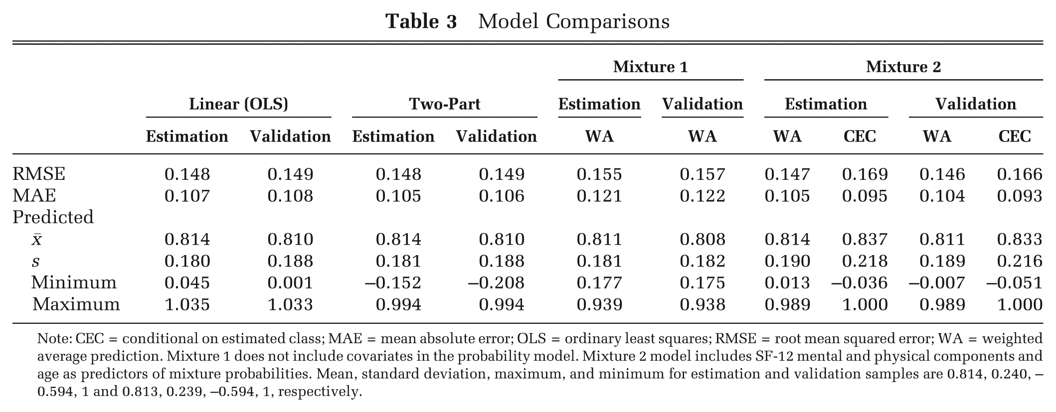
Note: CEC = conditional on estimated class; MAE = mean absolute error; OLS = ordinary least squares; RMSE = root mean squared error; WA = weighted average prediction. Mixture 1 does not include covariates in the probability model. Mixture 2 model includes SF-12 mental and physical components and age as predictors of mixture probabilities. Mean, standard deviation, maximum, and minimum for estimation and validation samples are 0.814, 0.240, –0.594, 1 and 0.813, 0.239, –0.594, 1, respectively.

Table 4

Prediction Performance in Validation Sample by Level of the EQ-5D-3L Index

								Mixture 2
		Linear (OLS)		Two-Part		Mixture 1		WA		CEC
EQ-5D-3L level	n	MAE	RMSE	MAE	RMSE	MAE	RMSE	MAE	RMSE	MAE	RMSE
All sample
<0	134	0.436	0.466	0.386	0.434	0.468	0.492	0.390	0.430	0.301	0.400
0–0.699	1241	0.179	0.226	0.177	0.235	0.194	0.239	0.174	0.232	0.191	0.286
0.7–0.899	2673	0.099	0.118	0.093	0.110	0.107	0.122	0.093	0.110	0.096	0.126
0.9–1	3073	0.072	0.095	0.076	0.100	0.090	0.100	0.072	0.095	0.040	0.100
All	7121	0.108	0.149	0.106	0.149	0.122	0.157	0.104	0.146	0.093	0.166
Diabetes, heart disease, or stroke
<0	62	0.366	0.400					0.333	0.378	0.241	0.351
0–0.699	437	0.179	0.224					0.173	0.226	0.189	0.288
0.7–0.899	411	0.106	0.130					0.092	0.114	0.073	0.100
0.9–1	240	0.103	0.130					0.104	0.130	0.078	0.134
All	1110	0.147	0.192					0.138	0.188	0.127	0.214

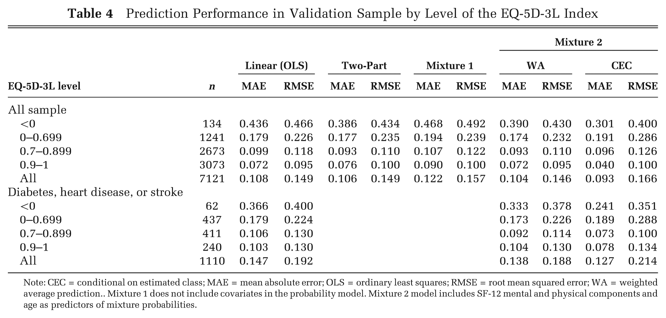
Note: CEC = conditional on estimated class; MAE = mean absolute error; OLS = ordinary least squares; RMSE = root mean squared error; WA = weighted average prediction.. Mixture 1 does not include covariates in the probability model. Mixture 2 model includes SF-12 mental and physical components and age as predictors of mixture probabilities.

Table 5 shows a cross-tabulation of observations classified based on the higher posterior and estimated probabilities using the validation sample and Mixture 2 estimates. The posterior classification (Equation 2) uses the observed EQ-5D-3L to calculate the probability that an observation belongs to 1 of the 3 classes and is thus the most accurate classification. From Table 5, approximately 75% of the observations are correctly classified when using the estimated probabilities for classification, which do not assume the EQ-5D-3L is observed. Observations away from EQ-5D-3L = 1 have a larger misclassification rate because the 2 Tobit components are close to each other and are thus harder to distinguish. These errors in misclassification produce larger RMSE.

Table 5

Classification Based on Posterior and Predicted Probabilities for Mixture 2 Model

Class Based on Posterior Probabilities	Class Based on Estimated Probabilities
Class Based on Posterior Probabilities	0	1	2
0	2538	534	1
0	(82.59)	(17.38)	(0.03)
1	880	2566	108
1	(24.76)	(72.20)	(3.04)
2	6	269	219
2	(1.21)	(54.45)	(44.33)

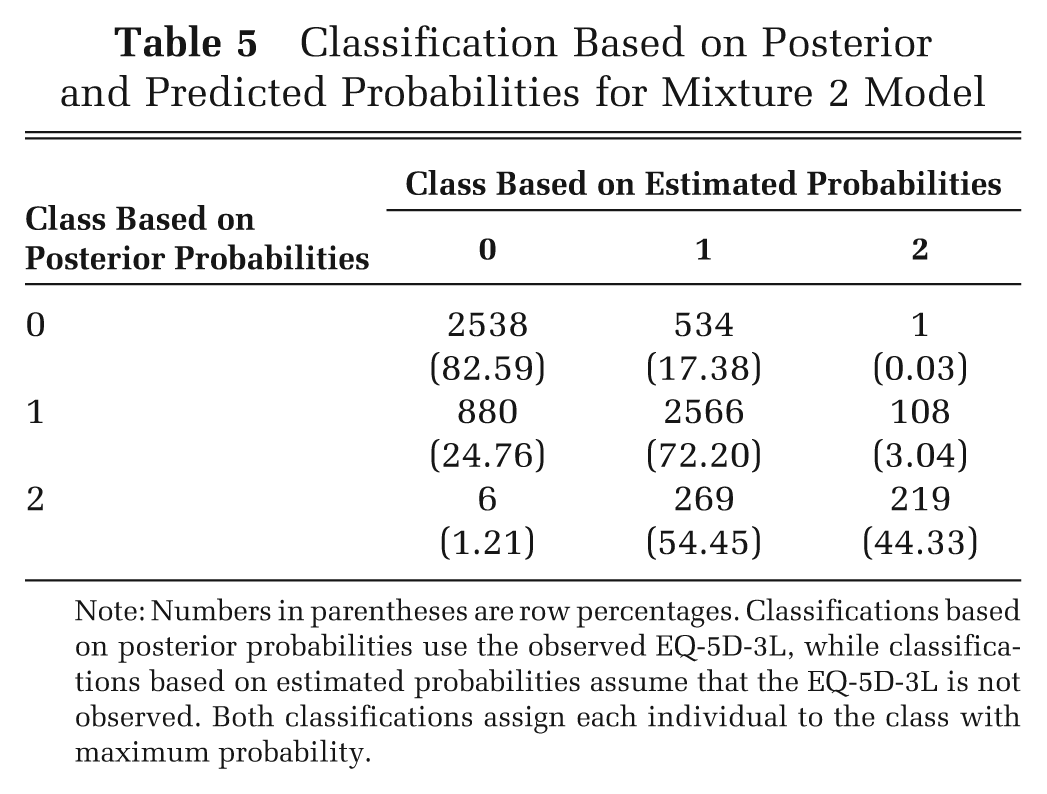
Note: Numbers in parentheses are row percentages. Classifications based on posterior probabilities use the observed EQ-5D-3L, while classifications based on estimated probabilities assume that the EQ-5D-3L is not observed. Both classifications assign each individual to the class with maximum probability.

Table 6 shows prediction comparisons for the linear (OLS) and Mixture 2 models (estimated coefficients not shown) for a subsample (n = 2219) of individuals who reported having diabetes, stroke, or heart disease, randomly divided into estimation (n = 1109) and validation (n = 1110) samples. As with models for the general population, RMSE gave a higher weight to larger errors, but based on MAE, both WA and CEC predictions are superior to those of the linear model. In particular, the MAE for CEC predictions represents a 14% improvement, from 0.147 to 0.127 in the validation sample. A finite mixture for this subpopulation makes better predictions than the linear model at the tails of the distribution, as can be seen from Table 4, although the mixture model underperforms in the interval 0–0.699. Predictions from the linear model regress toward the mean, overestimating the EQ-5D-3L for individuals with lower EQ-5D-3L while underestimating the EQ-5D-3L for those with higher observed values.

Table 6

Model Comparisons for Those with Diabetes, Heart Disease, or Stroke

			Mixture 2
	Linear (OLS)		Estimation		Validation
	Estimation	Validation	WA	CEC	WA	CEC
RMSE	0.197	0.193	0.194	0.225	0.188	0.214
MAE	0.150	0.147	0.144	0.137	0.138	0.127
Predicted
$\bar{X}$	0.654	0.658	0.654	0.670	0.658	0.677
s	0.252	0.245	0.252	0.300	0.246	0.288
Minimum	−0.003	−0.003	−0.035	−0.086	−0.035	−0.086
Maximum	1.031	1.043	0.985	1.000	0.989	1.000

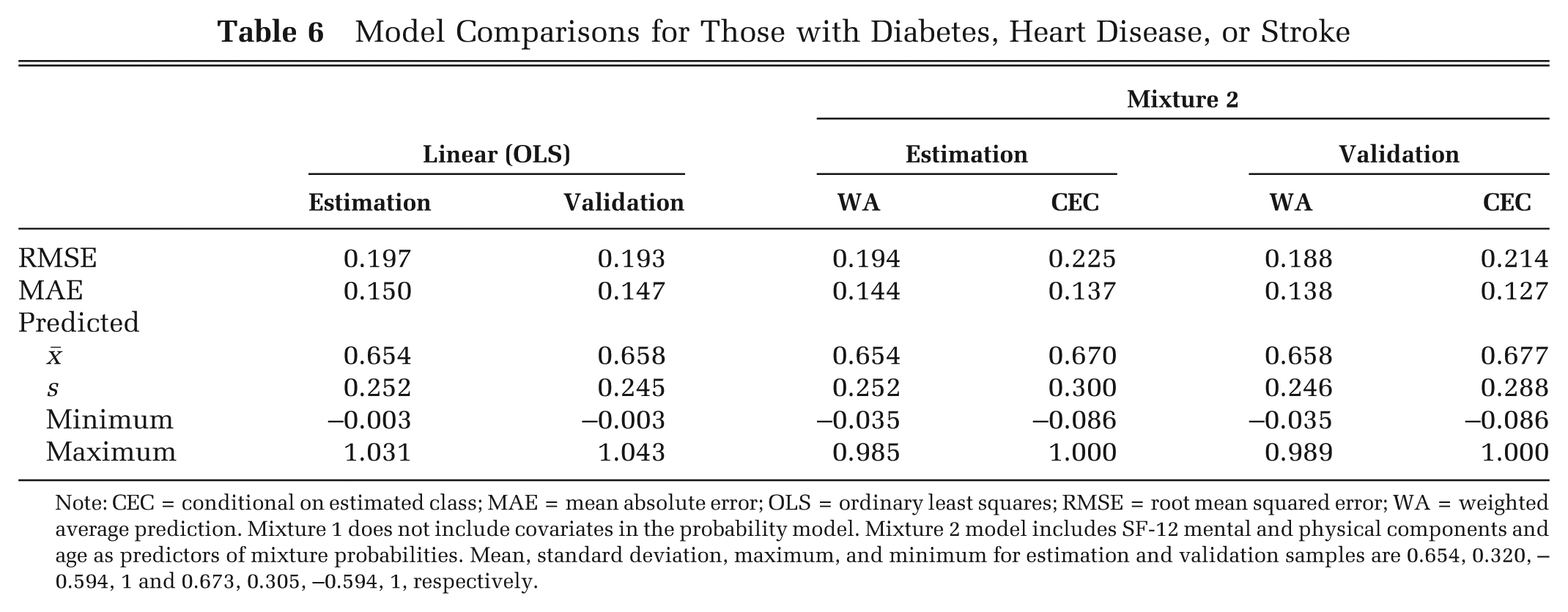
Note: CEC = conditional on estimated class; MAE = mean absolute error; OLS = ordinary least squares; RMSE = root mean squared error; WA = weighted average prediction. Mixture 1 does not include covariates in the probability model. Mixture 2 model includes SF-12 mental and physical components and age as predictors of mixture probabilities. Mean, standard deviation, maximum, and minimum for estimation and validation samples are 0.654, 0.320, –0.594, 1 and 0.673, 0.305, –0.594, 1, respectively.

Figure 2 shows the histograms of predicted values by model type. It can be seen that CEC predictions based on mixture models (Figure 2, bottom row) are able to reproduce the distribution of the observed data (Figure 1, A and I) more closely than are OLS and two-part models.

Figure 2

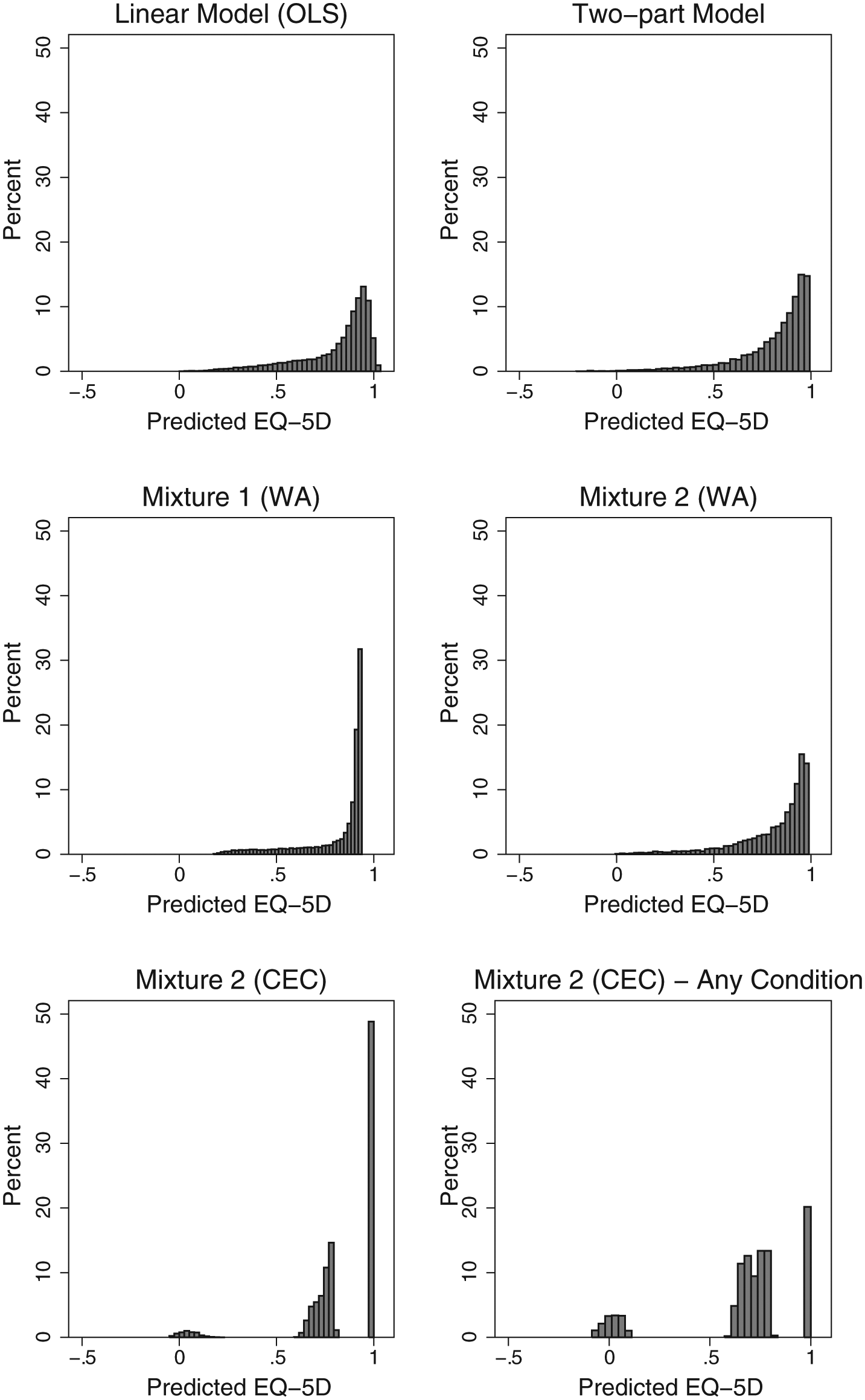
Histogram of predicted EQ-5D-3L scores by model. CEC = conditional on estimated class; WA = weighted average prediction. Mixture 1 does not include covariates in the probability model. Mixture 2 model includes SF-12 mental and physical components and age as predictors of mixture probabilities. Any condition includes respondents who reported having diabetes, heart disease, or stroke.

The best Mixture 2 model included only the SF-12 components as predictors of the mean EQ-5D-3L within each component (Table 2). Alternative models including age and sex fit the data well and could add more variability to the predictions, but the extra parameters that need to be estimated were penalized by the BIC. As a result, the most parsimonious model was preferred.

Discussion

The feasibility of economic evaluations is hindered if the data do not include preference-based measures. When data on preferences are not available, analysts use condition-specific or generic measures of health status to predict preferences. In this report, we showed that finite mixture models with Tobit components capture the idiosyncratic characteristics of the EQ-5D distribution, particularly when the sample does not include a large number of individuals in good health. Predictions from our best mixture model are superior at the tails of the distribution and on average, although some individuals can potentially be misclassified, which is reflected in larger RMSE. Moreover, linear and two-part models tend to perform better around the center of the observed distribution.

We use mixture models to account for a heterogeneous population even though the mixture components do not have a direct physical representation. Finite mixtures offer a flexible modeling approach that takes into account the characteristics of the distribution of societal preferences, which cannot be accurately described by a single probability density. Traditional methods, such as linear regression and two-part models, make poor predictions for extreme values of observed EQ-5D-3L scores and do not take into account the bounded nature of preference-based scores. As a consequence, these methods tend to overestimate preferences for individuals in the poorest health states while underestimating preferences for those individuals in the best health states, potentially biasing economic evaluations, which could then lead to misallocation of resources. In contrast, finite mixture models are able to improve prediction and mitigate biases at both tails of the distribution with only the SF-12 summary scores and age as predictors.

A known limitation of finite mixture models is that they tend to be difficult to estimate. When one is using maximum likelihood estimation, this problem is ameliorated by choosing appropriate starting values for the maximization algorithm regardless of the maximization method.³⁸ When we applied our strategy for choosing starting values to the MEPS dataset, however, model specifications converged to a global maximum and the estimated parameters were robust to the selection of starting values.

Another potential limitation is that there is no guarantee that mixture models will be appropriate for other datasets or that these datasets will have enough information to correctly separate observations into latent classes. For example, predicting societal preferences using general measures of health like the SF-12 is not as challenging as predicting individual preferences for those currently experiencing a particular health state. Individuals adapt to changes in their health status, and general measures of health may not provide enough information to estimate models as adaption may depend on unmeasured traits.³⁹ In our models, both SF-12 and age were sufficient to accurately predict class membership.

While Hernandez and others²⁶ demonstrated that mixture models can be used to predict EQ-5D-3L preferences using a measure of disability in a homogeneous clinic-based population with multiple observations per subject, our analysis shows that mixture models perform well using general health measures in a heterogeneous sample of the US population and cross-sectional data. Furthermore, we also demonstrated that mixture models are more useful when the target sample does not include a large proportion of individuals in good health. Our results using the SF-12 summary scores as predictors were consistent with those of Hernandez and others, which used a disability measure from the HAQ questionnaire and a pain measure as predictors and found improvements in both MAE and RMSE. However, our results show that mixture models do not outperform linear and two-part models over the whole range of observed EQ-5D values and that predictions based on classification may produce larger RMSE.

Finally, concerns have been expressed recently that mapping methods underestimate the observed variance of the EQ-5D-3L.⁴⁰ In OLS models, for example, predicted EQ-5D-3L values tend to regress toward the mean while the bulk of the observed values are away from it. However, when the EQ-5D-3L was predicted using mixture models and classification, the variances of observed and predicted EQ-5D-3L were closer in magnitude, although still underestimated but to a much smaller extent than the other methods.

Future research can exploit the richness of information available in the MEPS dataset to estimate mixture models for subpopulations with the same characteristics as those in datasets without preference-based measurements. To facilitate wider use of our proposed mixture models, we have made our Stata program publicly available (see Appendix A) and provide practical guidance on how to use our mixture models in Appendix B. Further research is also needed to evaluate under which conditions a finite mixture model produces better predictions on the whole range of observed EQ-5D-3L scores and whether additional refinement of mixture models can further improve predictions to better capture uncertainty.

Footnotes

Financial support for this study was provided in part by a training grant from the Agency for Healthcare Research & Quality (AHRQ) T32HS000084 (MCP) and a research grant R01HS020263 (YTS), also from AHRQ. The funding agreement ensured the authors’ independence in designing the study, interpreting the data, and writing and publishing the report.

Supplementary material for this article is available on the Medical Decision Making Web site at .

References

Drummond

Sculpher

Torrance

O’Brien

Stoddart

. Methods for the Economic Evaluation of Health Care Programmes. 3rd ed. New York: Oxford University Press; 2005.

Shaw

Johnson

Coons

. US valuation of the EQ-5D health states: development and testing of the D1 valuation model. Med Care. 2005;43(3):203–20.

Gold

. Cost-effectiveness in Health and Medicine. New York: Oxford University Press; 1996.

Szende

Oppe

Devlin

eds. EQ-5D Value Sets: Inventory, Comparative Review and User Guide. Dordrecht: Springer; 2010.

Oemar

Oppe

. EQ-5D-3L user guide, version 5.0 2013. Available from: URL: http://www.euroqol.org/fileadmin/user_upload/Documenten/PDF/Folders_Flyers/EQ-5D-3L_UserGuide_2013_v5.0_October_2013.pdf

Herdman

Gudex

Lloyd

. Development and preliminary testing of the new five-level version of EQ-5D (EQ-5D-5L). Qual Life Res. 2011;20(10):1727–36.

Gusi

Olivares

Rajendram

. The EQ-5D Health-Related Quality of Life Questionnaire. In: Preedy

Watson

, eds. Handbook of Disease Burdens and Quality of Life Measures. New York: Springer; 2010. p 87–99.

National Institute for Health and Clinical Excellence. Guide to the methods of technology appraisal 2013. Available from: URL: http://www.nice.org.uk/article/pmg9/resources/non-guidance-guide-to-the-methods-of-technology-appraisal-2013-pdf

Miller

Robinson

Lawrence

, Institute of Medicine. Committee to Evaluate Measures of Health Benefits for Environmental Health and Safety Regulation. Valuing Health for Regulatory Cost-effectiveness Analysis. Washington, DC: National Academies Press; 2006.

10.

Brazier

Kolotkin

Crosby

Williams

. Estimating a preference-based single index for the Impact of Weight on Quality of Life-Lite (IWQOL-Lite) instrument from the SF-6D. Value Health. 2004;7(4):490–8.

11.

Ware

Jr Kosinski

Keller

. A 12-Item Short-Form Health Survey: construction of scales and preliminary tests of reliability and validity. Med Care. 1996;34(3):220–33.

12.

Longworth

Rowen

. Mapping to obtain EQ-5D utility values for use in NICE health technology assessments. Value Health. 2013;16(1):202–10.

13.

Chuang

L-H

Kind

. Converting the SF-12 into the EQ-5D. Pharmacoeconomics. 2009;27(6):491–505.

14.

Craig

Pickard

Stolk

Brazier

. US valuation of the SF-6D. Med Decis Making. 2013;33(6):793–803.

15.

Brazier

Roberts

. The estimation of a preference-based measure of health from the SF-12. Med Care. 2004;42(9):851–9.

16.

Lundberg

Johannesson

Isacson

DGL

Borgquist

. The relationship between health-state utilities and the SF-12 in a general population. Med Decis Making. 1999;19(2):128–40.

17.

Lawrence

Fleishman

. Predicting EuroQoL EQ-5D preference scores from the SF-12 Health Survey in a nationally representative sample. Med Decis Making. 2004;24(2):160–9.

18.

Franks

Lubetkin

Gold

Tancredi

Jia

. Mapping the SF-12 to the EuroQol EQ-5D Index in a national US sample. Med Decis Making. 2004;24(3):247–54.

19.

Sullivan

Ghushchyan

. Mapping the EQ-5D index from the SF-12: US general population preferences in a nationally representative sample. Med Decis Making. 2006;26(4):401–9.

20.

Duan

Manning

Morris

Newhouse

. A comparison of alternative models for the demand for medical care. J Bus Econ Stat. 1983;1(2):115–26.

21.

. Some methodological issues with the analysis of preference-based EQ-5D index score. Health Serv Outcomes Res Method. 2009;9(3):162–76.

22.

Gray

Rivero-Arias

Clarke

. Estimating the association between SF-12 responses and EQ-5D utility values by response mapping. Med Decis Making. 2006;26(1):18–29.

23.

Brazier

Yang

Tsuchiya

Rowen

. A review of studies mapping (or cross walking) non-preference based measures of health to generic preference-based measures. Eur J Health Econ. 2010;11(2):215–25.

24.

Pullenayegum

Tarride

J-E

Xie

Goeree

Gerstein

O’Reilly

. Analysis of health utility data when some subjects attain the upper bound of 1: are Tobit and CLAD models appropriate?Value Health. 2010;13(4):487–94.

25.

Huang

Frangakis

Atkinson

. Addressing ceiling effects in health status measures: a comparison of techniques applied to measures for people with HIV disease. Health Serv Res. 2008;43(1 pt 1):327–39.

26.

Hernandez Alava

Wailoo

Ara

. Tails from the peak district: adjusted limited dependent variable mixture models of EQ-5D questionnaire health state utility values. Value Health. 2012;15(3):550–61.

27.

Longworth

Yang

Young

. Use of generic and condition-specific measures of health-related quality of life in NICE decision-making: systematic review, statistical modelling and survey. Health Technol Assess. 2014;18:1–224.

28.

Agency for Healthcare Research and Quality. Calculating the US population-based EQ-5D™ index score. Available from: URL: http://archive.ahrq.gov/professionals/clinicians-providers/resources/rice/EQ5Dscore.html

29.

Fleishman

. Demographic and clinical variations in health status: Agency for Healthcare Research and Quality. Available from: URL: http://meps.ahrq.gov/data_files/publications/mr15/mr15.pdf

30.

Lambert

. Zero-inflated Poisson regression, with an application to defects in manufacturing. Technometrics. 1992;34(1):1–14.

31.

McLachlan

Peel

. Finite Mixture Models. New York: Wiley; 2000.

32.

Enami

Mullahy

. Tobit at fifty: a brief history of Tobin's remarkable estimator, of related empirical methods, and of limited dependent variable econometrics in health economics. Health Econ. 2009;18(6):619–28.

33.

Tobin

. Estimation of relationships for limited dependent variables. Econometrica. 1958;26(1):24–36.

34.

Cameron

Trivedi

. Microeconometrics: Methods and Applications. Cambridge (UK): Cambridge University Press; 2005.

35.

Greene

. Econometric Analysis. Boston: Prentice Hall; 2012.

36.

Basu

Manca

. Regression estimators for generic health-related quality of life and quality-adjusted life years. Med Decis Making. 2012;32(1):56–69.

37.

Gould

Pitblado

Poi

. Maximum Likelihood Estimation with Stata. 4th ed. College Station, Texas: Stata Press; 2010.

38.

Karlis

Xekalaki

. Choosing initial values for the EM algorithm for finite mixtures. Comput Stat Data Anal. 2003;41(3–4):577–90.

39.

Chapman

Franks

Duberstein

Jerant

. Differences between individual and societal health state valuations. Med Care. 2009;47(8):902–7.

40.

Chan

KKW

Willan

Gupta

Pullenayegum

. Underestimation of uncertainties in health utilities derived from mapping algorithms involving health-related quality-of-life measures statistical explanations and potential remedies. Med Decis Making. 2014;34:863–72.

Supplementary Material

Please find the following supplemental material available below.

For Open Access articles published under a Creative Commons License, all supplemental material carries the same license as the article it is associated with.

For non-Open Access articles published, all supplemental material carries a non-exclusive license, and permission requests for re-use of supplemental material or any part of supplemental material shall be sent directly to the copyright owner as specified in the copyright notice associated with the article.

0.00 MB

0.04 MB

0.07 MB

Predicting the EQ-5D-3L Preference Index from the SF-12 Health Survey in a National US Sample

Abstract

Keywords

Background

EQ-5D-3L

SF-12

Previous Prediction Approaches

Methods

Data

Models

Analyses

Results

Discussion

Footnotes

References

Supplementary Material