
Abstract
Cost-effectiveness analyses (CEAs) of group-based interventions often use data from cluster randomized trials (CRTs). 1 A cluster design may be preferred in evaluations of interventions, which operate at a group level (e.g., alternative incentives for health providers), or where there is a high risk of “contamination” among the individuals within clusters (e.g., vaccination programs). 2,3 Agencies such as the National Institute for Health and Clinical Excellence may use these CEAs especially when recommending which public health interventions should be provided. 4 For these studies to provide a sound basis for decision making, appropriate statistical methods need to be developed and used. 5,6 CEAs based on randomized controlled trials (RCTs), where individual patients are randomized, have well-established methods. 7–9 However, statistical methods for CEAs of CRTs have received limited attention. 10 A review found that less than 10% of published CEAs of CRTs adopted appropriate statistical methods. 1
A distinct feature of CRTs is that the unit of randomization is the cluster (e.g., the hospital), not the patient. Each patient within a cluster is randomized to receive the same treatment, and so the form of clustering differs from multicenter RCTs, where patients within a center are randomized to different treatments. In CRTs, individuals within a cluster are likely to be somewhat similar in their characteristics and the care they receive, and therefore, individual outcomes or costs within the same cluster tend to be more homogeneous than those in different clusters. The extent of such clustering can be summarized by the intracluster correlation coefficient (ICC), which reports the proportion of the overall variation that is at the cluster level. For the analysis of clinical outcomes, it is recognized that ignoring clustering underestimates statistical uncertainty, 2,3,11 encourages incorrect inferences, 12–15 and can also lead to bias. 16,17 Appropriate methods for handling clustering in clinical outcomes are well developed and can include multilevel models (MLMs) and generalized estimating equations (GEEs). 18
CEAs of CRTs raise additional challenges for statistical methods. Here, methods are required that not only allow for clustering but also acknowledge the correlation between individual costs and outcomes 19–21 and make plausible assumptions about the distribution of costs and outcomes. Based on a conceptual review, we identified 4 main groups of statistical methods that may be appropriate for CEAs of CRTs: seemingly unrelated regression (SUR), 21 GEEs, 22 the nonparametric 2-stage bootstrap (TSB), 23 and MLMs. 20 Each of these methods can accommodate both clustering and correlation in a bivariate approach. We did not consider univariate net benefit regression analysis, as this method has less flexibility: for example, it does not allow for separate distributional assumptions to be made for costs (which tend to be highly skewed) as opposed to outcomes.
There is limited evidence comparing these alternative statistical methods for CEAs of CRTs. The TSB 24 and MLMs 25 have been proposed for CEAs of CRTs, but the only study 26 to compare these methods used data from a single CRT. A simulation study 24 assessed the performance of the TSB but did not compare it to MLMs or GEEs and assumed balanced clusters (equal numbers per cluster). It is therefore unclear which method performs best across the range of circumstances faced in CEAs of CRTs.
The aim of this article was to assess the relative performance of alternative statistical methods for CEAs of 2-arm CRTs. We address this by conducting an extensive simulation study and illustrate the practical use of the methods in a case study. In the next section, we describe each analytical method, the design of the Monte Carlo simulations, and the case study. We then present the results of the simulations and case study. The last section discusses the key findings and outlines an agenda for further research.
Methods
Statistical Methods for CEAs of CRTs
We consider 4 methods for CEAs that use CRT data. We use the following notation: let c ij and e ij represent the costs and outcomes for the ith individual in the jth cluster. For simplicity, the models and the simulation study are described for CEAs with 2 alternative treatments, but the models extend to evaluations with more than 2 randomized treatments. Each method takes the common approach of assuming linear additive treatment effects for both costs and outcomes. 9,20,21,27
Seemingly Unrelated Regression (SUR)
SUR consists of a system of regression equations that can recognize the correlation between individual costs and outcomes. 9,10,21 The SUR model 1 allows the individual-level error terms (ε) to be correlated through the parameter ρ:
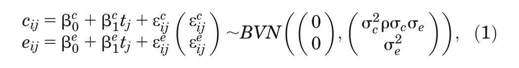
where tj
is the treatment indicator (tj
= 0 for control and 1 for treatment group). The parameters of interest, the incremental costs
A limitation of SUR is that its implementation in most standard statistical packages assumes the errors are normally distributed, which may not be plausible in the context of CEAs of CRTs. In addition, it is unclear whether the robust SE recognizes the correlation at the cluster level, that is, between cluster-level mean costs and mean outcomes. 29,30 Finally, the asymptotic assumptions underlying the robust variance estimator may not hold in CRTs with few clusters per treatment arm. 31 The problem can be exacerbated by skewed outcomes (or costs) or imbalanced cluster sizes. 18 More details on the robust variance estimator are given in Web Appendix 1.
Generalized Estimating Equations (GEEs)
A similar approach for handling clustering is to use a GEE model with robust SE. In general, GEEs offer a flexible extension of likelihood-based generalized linear models and are commonly used to analyze clinical outcomes in CRTs. 2,3,32 While multivariate GEEs have been developed to recognize potential correlation between binary end points, 22 they are complex to implement and have not been extended to continuous end points. As a practical alternative, we used a GEE model with independent estimating equations, stacking costs and outcomes, into a single vector but still allowing separate, independent estimates of incremental costs and outcomes. A bivariate GEE model with independent estimating equations can be written as:
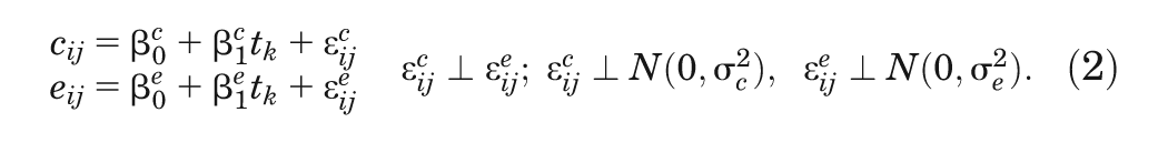
This structure relies on a general property of population-averaged GEEs, ensuring asymptotically consistent regression parameter estimates, even if the working correlation matrix is misspecified. This holds as long as the model, that is, the relationship between the marginal mean and the linear predictor, is correct. However, if the working correlation matrix is misspecified, the parameter estimates may be less statistically efficient.
Parameter estimates can be obtained by maximum likelihood, assuming that the errors have normal distributions, and can provide the same point estimates to OLS estimation. As with SUR, we assumed that the error terms have a bivariate normal distribution, although the model could be extended to allow for other distributions. We have used a robust estimator for the variance to allow for clustering when reporting uncertainty: see Web Appendix 1 for further details. However, the asymptotic properties required may not hold when there are few clusters. 13,15,33,65-68
The Nonparametric 2-Stage Bootstrap (TSB)
Nonparametric bootstrap methods can avoid parametric assumptions and are easy to apply in simple settings (e.g., RCTs). 19 However, the conventional nonparametric bootstrap that resamples individuals has to be extended to recognize the clustering inherent in CRTs. Davison and Hinkley 23 propose a 2-stage routine for CRTs, which resamples clusters as well as individuals, and this approach has been considered for CEAs. 24,26,34 The TSB can recognize the individual-level correlation between costs and outcomes by bivariate resampling, and the resampling can also stratify by treatment group. 24
TSB without shrinkage correction
One proposed TSB algorithm requires resampling clusters and then individuals within each resampled cluster (both with replacement). 23 The resultant data sets are used to calculate the statistics of interest, for example, incremental net benefits (INBs) and confidence intervals (CIs). However, unless the CRT has many clusters and individuals per cluster, this routine can overestimate the variance. Resampling at the second stage is likely to double count the within-cluster variance because the estimated cluster means from resampling at the first stage already incorporate both within- and between-cluster variability. 23,24,34
TSB with shrinkage correction
Davison and Hinkley 23 recommend a “shrinkage estimator” to correct for possible overestimation of the variance. Here, before any resampling, cluster means are calculated with a shrinkage correction and individual-level residuals estimated from the cluster means. Two-stage resampling (with replacement) is then performed by firstly resampling the shrunken cluster means and secondly resampling the standardized individual-level residuals across all clusters. Bootstrap data sets are compiled by combining the resampled shrunken cluster means and individual-level residuals. Unlike the previous routine where clusters and individuals are resampled from the original data, this routine resamples the shrunken means and residuals: see Web Appendix 2 for more details about the algorithms.
Both bootstrap routines rely on asymptotic assumptions, and it is unclear whether they are satisfied with few clusters, particularly if data are nonnormal. 35,36 Furthermore, the TSB routines described above were only proposed for balanced clusters, 23,24,34 which may make the method inappropriate for CEAs of CRTs with imbalanced clusters. 1 Our implementation therefore extends Davison and Hinkley’s original algorithms to allow for imbalanced clusters (Web Appendix 2).
Multilevel Models (MLMs)
MLMs can allow for the correlation between costs and outcomes and recognize clustering.
25
Unlike SUR, MLMs can explicitly recognize clustering by including additional random terms,
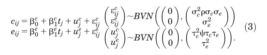
MLMs can be estimated and interpreted from a frequentist perspective, generally implemented with maximum likelihood or with a Bayesian approach typically using Markov chain Monte Carlo (MCMC) methods. Current software options for MCMC estimation afford a wide choice of distributional assumptions. 20 A concern with either approach is that the MLM may fail to converge if the CRT has few individuals per cluster. 37,38
Monte Carlo Simulations
Data-generating process
The simulation study was designed to test the methods across a wide range of circumstances typically found in CEAs of CRTs. Our conceptual review suggested it was important to allow the following to differ: number of clusters per treatment arm, number of individuals per cluster, level of cluster size imbalance, ICCs, skewness in the cost distribution, and correlation between costs and outcomes at both the individual and cluster level (see rationale in Table 1). To consider this range of settings required a flexible data-generating process. Data were constructed to reflect the specific form of clustering found in CRTs. 12,37,39 The design allowed for a wide range of parameters to be varied and could accommodate different parametric distributions for costs and outcomes. As in previous simulation studies in economic evaluation, we assumed a linear additive treatment effect throughout. 21,24,40 We simulated cost (c) and outcome data (e) from CRTs with M clusters per arm and n m (m = 1. . .M) individuals per cluster. Data were generated firstly at the cluster level and then at the individual level according to equation 4 below.
Description, Rationale, and Evidence for the Parameter Values Allowed to Vary across the Different Scenarios
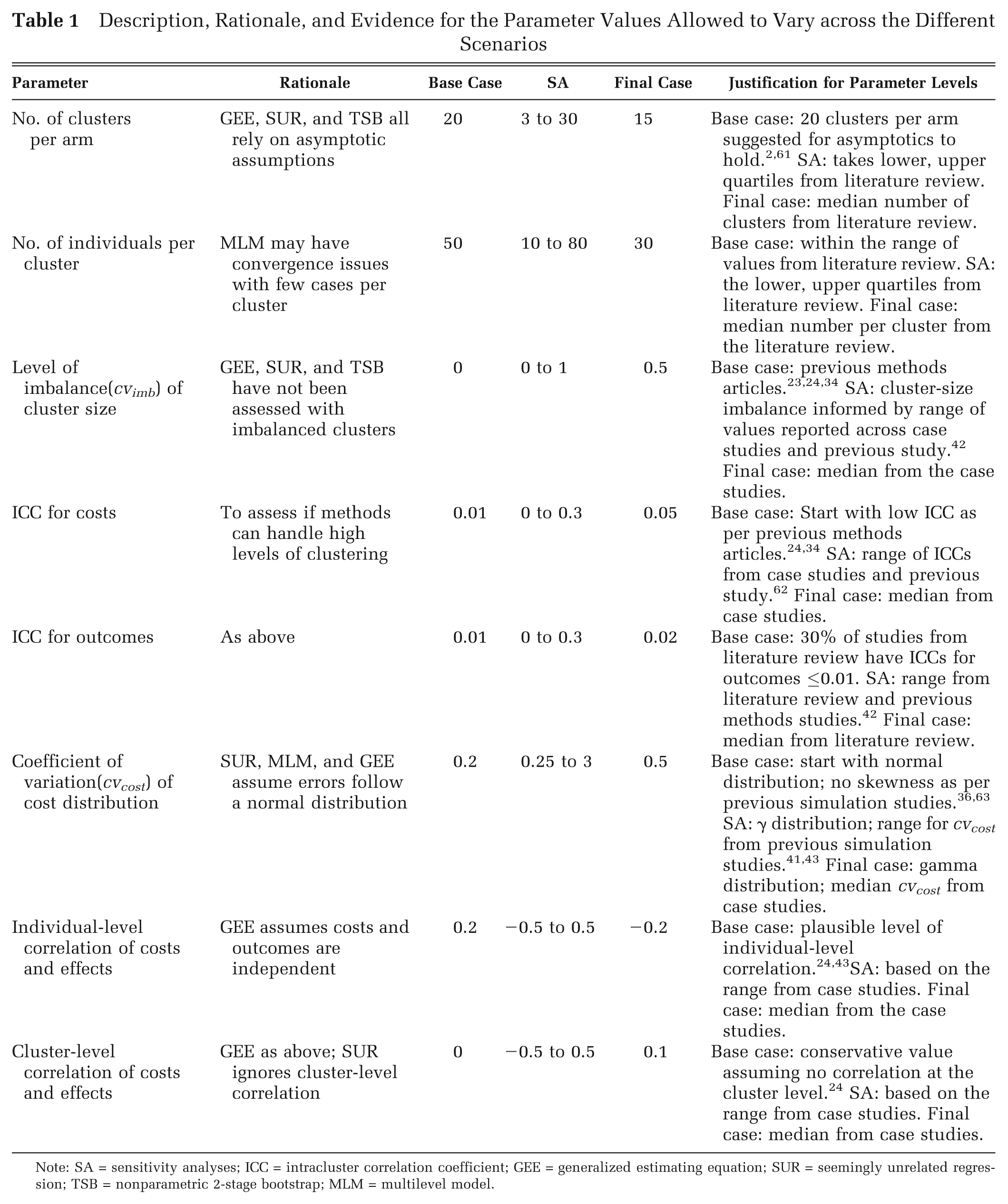
Note: SA = sensitivity analyses; ICC = intracluster correlation coefficient; GEE = generalized estimating equation; SUR = seemingly unrelated regression; TSB = nonparametric 2-stage bootstrap; MLM = multilevel model.
Cluster level means:

Individual-level data:
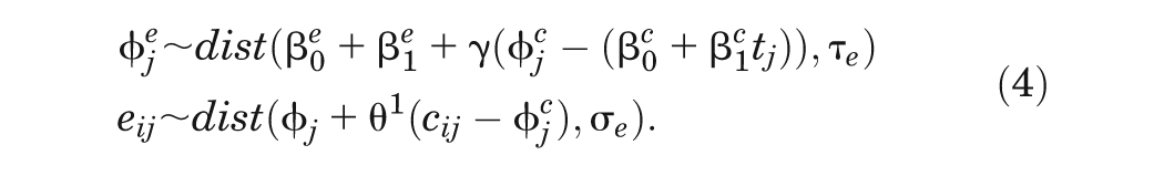
Cluster-level mean costs
Definition of scenarios
The simulation study initially considered a base-case scenario, then 1-way and multiway sensitivity analyses, and finished with a final “most realistic” scenario. Under the base-case scenario, parameter values were chosen not only to be plausible but also to represent circumstances where each method was anticipated to perform well. This scenario provided a benchmark for the subsequent sensitivity analyses (Table 1). The choices of which parameters to vary in the sensitivity analyses, and which scenarios to combine in the multiway sensitivity analyses, were informed by general insights from the methods literature. For each parameter, the range of values chosen was grounded in a systematic literature review of 62 studies, 1 previous methods articles and simulation studies, 24,41–43 and 8 case studies. 44–51 In the final scenario, each parameter was set to its “most realistic” value, taking median values from the literature review and case studies. For example, costs followed a normal distribution in the base case but increasingly skewed gamma distributions in the sensitivity analyses with coefficient of variation (cv cost ) ranging from 0.25 to 3.0 (final case, 0.5).
Table 1 lists the parameters changed across the scenarios; other parameters such as the true incremental costs and outcomes (QALYs) were held constant throughout. For example, the “true” incremental costs, incremental QALYs, and INBs (assuming a threshold of £20,000 per QALY) were £500, 0.075, and £1000, respectively.
Implementation
The performance of the different estimation methods was assessed according to mean (SE) bias, root mean squared error (rMSE), CI coverage, the error rate for lower and upper CI limits, and CI width (see Web Appendix 3 for definitions). We used 2000 simulations for each scenario.b The performance of each method in estimating incremental costs, incremental QALYs, and INBs was reported.
MLM, GEE, and TSB were implemented in R 52 and SUR in STATA (StataCorp). 53 The SUR was estimated by IFGNLS, without and with a robust SE. The GEE was estimated with a robust SE, and the TSB was estimated before and then after shrinkage correction. The MLM was estimated by maximum likelihood across all scenarios. 65 For selected scenarios (base case, 3 clusters per treatment, and the final case), estimation was also carried out via MCMC by calling WinBUGS from R. 54 The MCMC estimation consisted of 5000 iterations, 3 parallel chains with different starting values, and assuming diffuse priors. 55
Case Study
To consider the potential implications of the choice of methods in practice, we compared the methods in a case study of a CEA alongside a CRT. This approach extends the simulation study as, for example, the cost and outcome data do not follow specified distributions; this allows for a more pragmatic comparison of the methods. We compare estimates of both relative cost-effectiveness and potential value of further research across the methods. The potential value of further research is the gain from resolving decision uncertainty, given the current state of knowledge. In other words, the expected value of perfect information (EVPI) is the increase in net benefits from taking the optimal decision after resolving current uncertainty. 56
The case study consists of a CRT that evaluates an educational intervention intended to improve the management of lung disease in adults attending outpatient clinics in South Africa. 46 The CRT included 40 balanced clusters (clinics) randomized to intervention or control. This reanalysis used complete data for 1851 patients. For each patient, the study measured health service costs for 3 months, consisting mainly of the costs of the educational intervention clinic, outpatient visits, and drugs. EQ-5D data were recorded at 3 months’ follow-up, and we calculated QALYs, assuming that there was no mortality. The ICCs for costs and outcomes were both low (around 0.01). While the outcome data were approximately normally distributed, the costs were moderately skewed (cv cost = 1.6). Hence, the characteristics of this study were fairly similar to those in the base-case scenario in the simulation.
Each of the above statistical methods were used to report incremental costs, QALYs, and INBs, calculated at realistic levels of the ceiling ratio for the local South African context. We then used these estimates across the alternative methods to compare the EVPI per patient, as reported in other trial-based CEAs. 57,58 EVPI was calculated assuming that the INB was normally distributed. 56
Results
Simulation Study
Base case
In the base case, each method reported low bias and similar rMSE for the INB (Table 2). The method that ignored clustering, SUR without the robust SE, performed poorly with CI coverage below 0.9. The TSB without shrinkage correction reported wide 95% CIs and coverage above the nominal level, but with correction, coverage was similar to the other methods that recognized clustering. The MLM had coverage close to the nominal level whether estimated by maximum likelihood (Table 2) or MCMC (CI coverage, 0.94). The relative performance across methods was similar for incremental QALYs, incremental costs, and INBs calculated with alternative levels of the ceiling ratio.
Bias, rMSE, CI Coverage, and Width of the Mean INB for the Base Case (True INB = £1000)
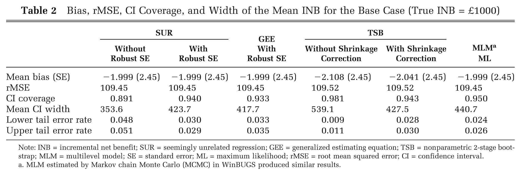
Note: INB = incremental net benefit; SUR = seemingly unrelated regression; GEE = generalized estimating equation; TSB = nonparametric 2-stage bootstrap; MLM = multilevel model; SE = standard error; ML = maximum likelihood; rMSE = root mean squared error; CI = confidence interval.
MLM estimated by Markov chain Monte Carlo (MCMC) in WinBUGS produced similar results.
One-way sensitivity analysis
The bias was low across all scenarios; for example, in the scenario with 3 clusters per treatment arm, the mean (SE) biases for the estimated INB were −9.98 (6.05) for SUR, –6.93 (6.28) for the MLM and GEE, and −7.15 (6.29) for the TSB with shrinkage correction (true INB = £1000). The rMSE differed across scenarios but was similar for each method. For example, with 3 clusters per arm, rMSE was about 280 for all methods.
Table 3 reports CI coverage for the 1-way sensitivity analyses. The bootstrap without correction reported CI coverage above the nominal level for most scenarios, but the other methods generally reported good coverage, unless there were few clusters. Here, CI coverage remained good for the MLM and TSB (following correction), but the SUR and GEE, both with robust SEs, reported poor coverage. With high levels of cluster size imbalance, coverage levels for these latter 2 methods were also low. All the methods (except the TSB without correction) performed well in scenarios with few individuals per cluster, high ICCs, and highly skewed costs (Table 3). CI coverage also remained close to the nominal level, with high levels of correlation at the individual or cluster level.
Confidence Interval Coverage of the Mean Incremental Net Benefit (Nominal Level Is 0.95) for the 1-Way Sensitivity Analyses
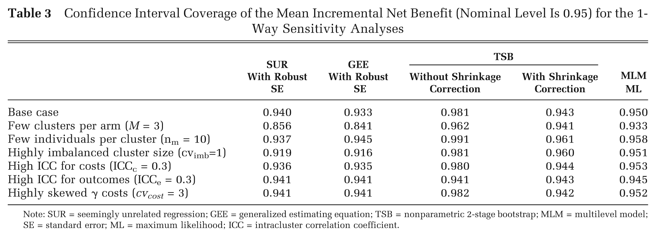
Note: SUR = seemingly unrelated regression; GEE = generalized estimating equation; TSB = nonparametric 2-stage bootstrap; MLM = multilevel model; SE = standard error; ML = maximum likelihood; ICC = intracluster correlation coefficient.
Multiway sensitivity analysis
The multiway sensitivity analyses combined variation in the number of clusters, levels of cluster size imbalance, and cost skewness. Bias remained low (between −5 and 5) across all multiway sensitivity analyses. While rMSE increased when fewer clusters were combined with high levels of imbalance, the differences between methods were small.
Figure 1 reports CI coverage for CRTs with decreasing number of clusters (20, 15, 10, 8, 5, and 3 clusters per treatment arm), moderate and high cluster-size imbalance (cvimb of 0.5 and 1), combined with highly skewed costs (cv cost = 3). In CRTs with moderate levels of imbalance, the performance of SUR and GEE is worse than for the MLM and TSB if there are 8 or fewer clusters per treatment arm (Figure 1A). With high levels of cluster size imbalance, the coverage levels for the SUR and GEE are poor, with fewer than 10 clusters per arm (Figure 1B). For the MLM and TSB (with shrinkage correction), the CI coverage remains relatively good even when the study has few highly imbalanced clusters and highly skewed costs. In further scenarios that combined variation in cluster-size imbalance and number of clusters with other parameters, such as different levels of individual- and cluster-level correlation, all methods performed well except in scenarios with few clusters, where SUR and GEE reported poor coverage.
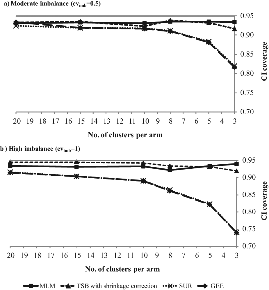
CI coverage (nominal level is 0.95) for multiway sensitivity analyses: high skewness of costs (cv cost = 3), decreasing number of clusters combined with (A) moderate and (B) high cluster-size imbalance. The CI coverage is very similar for the GEE and SUR, and hence, their lines show considerable overlap.
Final “most realistic” scenario
In the final scenario with all parameters set to their “most realistic” levels (Table 1), bias and rMSE were again similar across methods (Table 4). The SUR without a robust SE and the TSB without correction reported levels of CI coverage that diverged from the nominal, but the MLM and TSB with correction both had good levels of CI coverage.
Bias, rMSE, CI Coverage, and Width of the Mean INB for the Final Case (True INB = £1000)
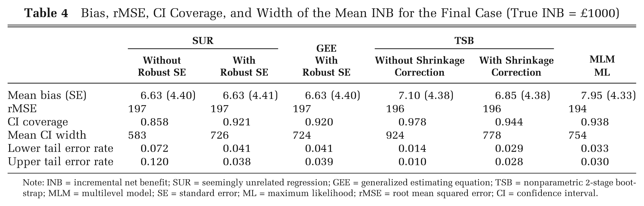
Note: INB = incremental net benefit; SUR = seemingly unrelated regression; GEE = generalized estimating equation; TSB = nonparametric 2-stage bootstrap; MLM = multilevel model; SE = standard error; ML = maximum likelihood; rMSE = root mean squared error; CI = confidence interval.
Case Study
Table 5 presents cost-effectiveness results from applying the alternative methods to the case study. Each method reported that the intervention had positive incremental costs, negative incremental QALYs, and negative INBs. While the means were similar across methods, applying SUR without allowing for clustering led to standard errors that were substantially smaller than for the other methods. For SUR without the robust errors, the EVPI (per patient) was more than 50% lower when compared to methods that accommodate clustering.
Case Study Results: Incremental Cost, Incremental QALY, INB (Threshold of R100,000 per QALY), a and Individual EVPI
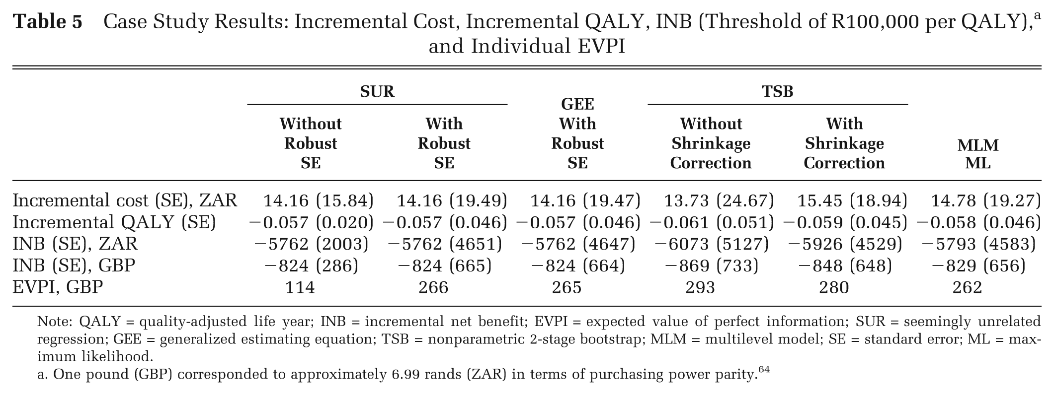
Note: QALY = quality-adjusted life year; INB = incremental net benefit; EVPI = expected value of perfect information; SUR = seemingly unrelated regression; GEE = generalized estimating equation; TSB = nonparametric 2-stage bootstrap; MLM = multilevel model; SE = standard error; ML = maximum likelihood.
One pound (GBP) corresponded to approximately 6.99 rands (ZAR) in terms of purchasing power parity. 64
Discussion
This study compares the relative merits of alternative statistical methods for CEAs of CRTs. The simulation study finds that each method reports low bias and similar MSE across the settings considered, with the MLM and TSB (with correction) providing good levels of CI coverage throughout. The simulation study highlights that robust methods (SUR and GEE), which rely on asymptotic assumptions, can perform poorly for studies with few clusters. Both the simulation study and the case study illustrate that methods that ignore clustering (e.g., SUR without a robust SE) can seriously underestimate statistical uncertainty. As our empirical example illustrates, ignoring clustering can therefore understate the expected value of further research. Future studies should not attempt to justify statistical methods that ignore clustering on the basis of low estimated ICCs.
This is the first article to compare a range of statistical methods for CEAs of CRTs. Previous simulation studies 24,34 did not consider MLMs or GEEs, and other studies just compared the methods using a single case study. 26 The design of the simulation study is sufficiently general to consider the methods across common circumstances faced by CEAs of CRTs. In particular, the simulation includes scenarios with few clusters, unequal numbers per cluster (imbalance), and highly skewed costs. The choice of scenarios and parameters values are grounded in a previous review of methods and of published CEAs of CRTs. 1 These features help ensure that the simulation study provides relevant insights on the choice of analytical method for future CEAs. While for illustrative purposes we consider 2-armed CRTs, the findings extend directly to CRTs with 3 or more randomized treatments.
The simulation study finds the TSB performs as well as the MLM across the circumstances considered, once the shrinkage correction factor proposed by Davison and Hinkley is applied. A previous CEA used the TSB, but did not apply the shrinkage correction, and reported wide CIs compared to a MLM. 26 We find that without the shrinkage correction, the TSB overstates the uncertainty, but once the correction is applied, the method gives good CI coverage. This finding contrasts with those of a previous simulation study 24 that only considered balanced clusters but reported relatively poor performance for the TSB (even after correction). We extended the implementation to recognize cluster-size imbalance and find that the method still performs well. To help improve the translation of appropriate methods into practice, we are developing user-friendly software for implementing the TSB. Sample codes for the TSB, GEE, and MLM are included in Web Appendix 4.
This article considers GEEs for the first time in this context. We develop a robust variance estimator to account for the clustering that also allows for the joint distribution of individual costs and outcomes. A general concern for such a robust variance estimator is that it relies on asymptotic assumptions, which in these circumstances pertain to the number of clusters per treatment arm. Our work provides specific guidance for CEAs of CRTs on the number of clusters per treatment arm required for asymptotic assumptions to hold. Our findings suggest that between 8 and 15 clusters per arm are required, depending on the other features of the study; in particular, more clusters are required when the cluster sizes are highly imbalanced. This is pertinent for CEAs where about 40% of such studies have fewer than 15 clusters per treatment arm and 15% less than 8 clusters. 1 The general literature on GEEs has reported similar sample size requirements for asymptotic assumptions to hold, 13,15,18 and the same requirements apply to the robust estimator for SUR. The simulation study also finds that the performance of these methods does not improve in CRTs with more individuals per cluster.
Grieve and others 25 proposed a flexible Bayesian hierarchical model to tackle the main statistical issues faced by CEAs of CRTs. However, such models are complex to implement, and other more accessible MLMs may be required to improve practice. Our simulation showed that a MLM estimated by maximum likelihood, assuming a bivariate normal distribution for costs and outcomes, can perform well even when costs are highly skewed. Although in a different context, this corroborates previous findings that suggest methods assuming normality may be quite robust to skewed cost data. 21,40,41,43 However, it would be worth investigating whether MLMs that better accommodate skewed costs would lead to gains in precision.
This study has several limitations. While the simulation considers a wide range of circumstances and the case study provides a useful illustration, in practice, some CEAs face further complications. If, for example, there are baseline imbalances between the treatment groups, or cost-effectiveness estimates are required for particular subgroups, the methods would need to consider covariates. The effects of baseline covariates, and indeed treatment group, on costs and outcomes may be multiplicative, not additive. 59 Also, CEAs may have more complex variance structures than those considered. 25,60 These methods have not been tested under such circumstances, but MLMs may have more scope for adaptation to these broader settings than the other methods. 18,20,21,43 In addition, we have not considered censored or missing data or combining CRT data with evidence from other sources in decision models. These are all avenues for further research.
In conclusion, CEAs of CRTs may inform recommendations on the provision of area-level or public health interventions. This study finds that MLMs and TSB (with correction) are appropriate analytical methods for CEAs of CRTs across a wide range of circumstances. While methods that use a robust variance estimator such as SUR and the GEE model considered here are simple to implement, they are not recommended for CEAs of CRTs with few (less than 10) clusters in each treatment arm.
Footnotes
Acknowledgements
The authors are grateful to Simon Dixon and John Cairns for helpful comments and Max Bachmann for providing access to the Outreach data. They also thank participants including the discussant Joshua Pink at the Health Economists’ Study Group meeting (University of York, January 2011), where an earlier version of this work was presented. Finally, they thank the collaborators on the study—Graham Scotland, Patrick Gillespie, Allan Clark, and Mike Gillett—for useful discussions.
This work was presented at the Health Economists’ Study Group meeting; January 2011; York, UK.
Financial support was from a UK Medical Research Council Grant (ESWN, RG) and a PhD scholarship from Fundação para a Ciência e a Tecnologia (MG).
References
Supplementary Material
Please find the following supplemental material available below.
For Open Access articles published under a Creative Commons License, all supplemental material carries the same license as the article it is associated with.
For non-Open Access articles published, all supplemental material carries a non-exclusive license, and permission requests for re-use of supplemental material or any part of supplemental material shall be sent directly to the copyright owner as specified in the copyright notice associated with the article.