
Abstract
This study advances the field of Computationally Intensive Theory Development (CTD) by examining the capabilities of Explainable Artificial Intelligence (XAI), in particular SHapley Additive exPlanations (SHAP), for theory development, while providing guidelines for this process. We evaluate SHAP’s methodological abilities and develop a structured approach for using SHAP to harness insights from black-box predictive models. For this purpose, we leverage a dual-methodological approach. First, to assess SHAP’s capabilities in uncovering patterns that shape a phenomenon, we conduct a Monte-Carlo simulation study. Second, to illustrate and guide the theory development process with SHAP for CTD, we apply SHAP in a use-case using real-world data. Based on these analyses, we propose a stepwise uniform and replicable approach giving guidance that can benefit rigorous theory development and increase the traceability of the theorizing process. With our structured approach, we contribute to the use of XAI approaches in research and, by uncovering patterns in black-box prediction models, add to the ongoing search for next-generation theorizing methods in the field of Information Systems (IS).
Keywords
Introduction
Computationally Intensive Theory Development (CTD) emphasizes the use of computational methods, for pattern detection as initial input for subsequent abductive theorizing and theory development (Abbasi et al., 2023; Berente et al., 2019; Lindberg, 2020; Miranda et al., 2022a; Shrestha et al., 2021). Essentially, CTD approaches encourage researchers to (re-)analyze complex and extensive data using computational methods to discover new insights that complement extant knowledge, and ultimately formulate advanced theories for phenomena under investigation through abductive reasoning on what real-world mechanisms generated the observed patterns (Behfar and Okhuysen, 2018; Miranda et al., 2022a; Zhang et al., 2022). Machine Learning (ML) is particularly promising for pattern detection due to its high efficiency in detecting patterns in vast datasets (Choudhury et al., 2021; Lindberg, 2020; Shmueli and Koppius, 2011; Shrestha et al., 2021). However, the methodological guidance on ML in CTD is very limited, despite manuscripts offering the conceptual foundations for CTD (Berente et al., 2019; Lindberg, 2020; Miranda et al., 2022a) and studies that provide initial application advice (Choudhury et al., 2021; Shrestha et al., 2021; Zhang et al., 2022). This limits researchers’ use of ML in CTD approaches for theory development. Yet, application frameworks could provide structured foundations for using ML in CTD and for advancing the corresponding research methodology (Burton-Jones et al., 2021; Padmanabhan et al., 2022; Von Krogh et al., 2023).
The limited available literature offers valuable but context-specific approaches giving initial yet constrained advice regarding the use of computational methods such as ML in CTD. Zhang et al.’s (2022) seminal study, for example, develops a framework for theorizing organizational routines, using sequential process mining to identify patterns in processes as a basis for abductive theory development. Shrestha et al. (2021) offer a more broadly applicable approach by demonstrating how ML can disclose patterns in data and how scholars can evaluate them for robustness using traditional statistical methods as basis for abductive theorizing. Both studies mentioned, yet did not explicitly explore, the interpretability of ML models in-depth. Particularly, interpretability is crucial for CTD, since human understanding of ML-detected patterns and subsequent theory construction is dependent on these patterns being represented in a form that humans can interpret. Defining interpretable ML merely as such ML algorithms that generate interpretable models by design (Barredo Arrieta et al., 2020; Rudin, 2019), both studies suggest excluding algorithms that generate black-box models (Shrestha et al., 2021; Zhang et al., 2022), despite complementary approaches, so-called Explainable Artificial Intelligence (XAI), that allow for the approximation and interpretation of black-box models (Barredo Arrieta et al., 2020; Gunning et al., 2019). Thereby, CTD literature exhibits a gap regarding highly effective, yet opaque black-box models developed by using algorithms, such as Artificial Neural Networks (ANN) (Hassoun, 1995), and the XAI approaches to make them interpretable.
This gap is remarkable, considering that state-of-the-art ML algorithms generate black-box models that have been shown to be highly effective in uncovering novel and valuable patterns (Asatiani et al., 2021; Sturm et al., 2021; Zhao and Hastie, 2021). Many such models are particularly effective in detecting nonlinear patterns and other previously unknown relationships in data, which are not easily identifiable using other methods (Kim et al., 2023; Lindberg, 2020; Tidhar and Eisenhardt, 2020). For such black-box models, XAI can provide relevant, easily understandable, and straightforwardly interpretable insights into patterns (Barredo Arrieta et al., 2020). Further, the general exclusion of XAI-based approaches is notable, considering the widespread use and discussion of XAI approaches, such as SHAP, in computer science and Information Systems (IS) research (Bauer et al., 2023; Fernández-Loría et al., 2022; Gramegna and Giudici, 2021; Xie et al., 2023; Zacharias et al., 2022). Using XAI makes insightful empirical patterns interpretable, thus potentially offering input to advance extant or develop new theories in fields where vast datasets are available—typically highly digital settings which are common in the IS field (Berente et al., 2019; Maass et al., 2018). The value of combining black-box ML models and XAI is emphasized, for instance, by their use in discovering new drugs through the detection of patterns in molecules (Jiménez-Luna et al., 2020; Webel et al., 2020), in explaining employee turnover based on human resource data (Choudhury et al., 2021; Chowdhury et al., 2023), or in developing superior production processes based on patterns in manufacturing data (Senoner et al., 2022).
Overall, the gaps in the literature on XAI use and its limitations with respect to theorizing manifests in a small number of methodologically focused papers that provide guidance for XAI application in theorizing. We found one notable exception in Choudhury et al. (2021), who discuss how to exploit different ML models, including black-boxes, combined with XAI, to detect patterns in predictions visually, also allowing abductive reasoning based on them. Their study offers detailed suggestions on crucial steps for ML use in pattern detection; however, it does not elaborate in-depth on consideration of the use, capabilities, and limitations, nor on the interpretation of the XAI approach they used. Additionally, linking XAI-detected patterns to theorizing is only discussed very briefly, since these aspects are not the central focus of the study. Similarly, studies investigating the use (e.g., Senoner et al., 2022; Zacharias et al., 2022) and limitations of XAI tools, such as Shapley Additive Explanations (SHAP) (e.g., Fernández-Loría et al., 2022), do not link their insights to theorizing.
Consequently, there is no solid foundation upon which researchers can integrate black-box ML models with XAI into their toolkit for theory development. Therefore, the potential contribution this combination holds for research, also in complementing glass-box models, is not exploited. To address this gap and to provide a guideline for using XAI in pattern detection for theory development, we investigate the use and limitations of a particular XAI approach: SHAP (Lundberg and Lee, 2017). This approach reveals variable impacts in black-box models, thus offering insight on patterns and phenomena embedded in the data, through various plots and visualizations (Lundberg et al., 2018). Since SHAP is a model-agnostic approach (Gramegna and Giudici, 2021; Ribeiro et al., 2016), it is particularly promising due to its application being independent of the underlying ML model (Barredo Arrieta et al., 2020; Lundberg and Lee, 2017). This produces comparable and consistent outputs across different ML models, to potentially facilitate a transparent, comprehensible, and replicable pattern detection for the theory-building process. Considering the versatility of SHAP and its widespread use, it is promising as a CTD tool and, consequently, for our investigation on the use of XAI for CTD. Shedding light on its use and limitations of its use, we pose the following research question: How and under what circumstances can XAI, and particularly SHAP, be used to detect patterns for Computationally Intensive Theory Development?
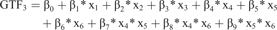
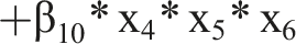
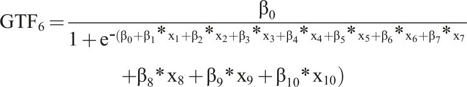
In answering this question, we first simulate datasets for multiple phenomena described by predefined ground truth functions (GTFs), a mathematical function that defines an observable outcome. These GTFs vary in complexity (e.g., comprising different interaction effects and nonlinear relationships) and involve common real-world data shortcomings such as random error terms. We analyze conditions under which SHAP provides good representations of the GTFs and those under which it systematically decreases output quality. This first part of our study aims to uncover limitations of the approach and to indicate when it can be used confidently. Next, we apply SHAP to analyze an empirical dataset, showing how it can be used to detect patterns and how to abductively transform them to theory.
We illustrate the trade-off between a SHAP values threshold for variable relevance and the predictive performance an ML model reaches for confident pattern detection using SHAP. Additionally, we develop a seven-step guideline for using SHAP effectively in CTD. Our framework utilizes SHAP to add black-box models as a valuable extension of the toolkit for CTD to inspire new theorizing and theory development. This study adds to the controversial discussion on the use of black-box ML models and the applicability of XAI, particularly of SHAP, in research (Fernández-Loría et al., 2022; Rudin, 2019; Shrestha et al., 2021; Smith, 2020; Zhang et al., 2022). Further, we contribute to the discussion on CTD in IS research (Berente et al., 2019; Lindberg, 2020; Miranda et al., 2022a) by shedding light on the role of XAI in next-gen theory development in IS research (Burton-Jones et al., 2021; Grover and Lyytinen, 2023).
Computationally intensive theory development—Computationally detected patterns for abductive theorizing
CTD refers to approaches in which computational methods are used to disclose patterns in empirical data, which can aid humans in abductive theory development (Abbasi et al., 2023; Berente et al., 2019; Lindberg, 2020; Miranda et al., 2022a; Shrestha et al., 2021). By combining computational methods and human cognition, we can exploit the strengths of both components (Berente et al., 2019; Grisold et al., 2024; Lindberg, 2020). While computational approaches are highly efficient in detecting patterns, even in overwhelmingly large datasets that exceed human cognition (Berente et al., 2019; Lindberg, 2020; Zhang et al., 2022), humans can critically assess patterns that exhibit statistical artifacts or spurious patterns, and develop plausible explanations that add to understanding observable phenomena (Maass et al., 2018; Miranda et al., 2022a; Zhang et al., 2022). Since CTD approaches aid theory development on vast datasets (Maass et al., 2018; Tonidandel et al., 2018), they are particularly well suited for digital environments producing extensive data such as trace data or machine generated data, as well as for (re-)using secondary data sources (Berente et al., 2019).
Computationally detected patterns—discernible regularities in empirical data (Lindberg, 2020; Miranda et al., 2022a) in the form of specific relationships between variables (Shrestha et al., 2021)—are at the heart of CTD. The patterns build the basis for investigating and theorizing phenomena. ML is a particularly promising computational method for uncovering patterns (Choudhury et al., 2021; Miranda et al., 2022a; Tonidandel et al., 2018) because it builds models of relations between variables, to accurately predict an outcome variable 1 (Choudhury et al., 2021). Analyzing these models allows the disclosure of potentially relevant variables (Zhao and Hastie, 2021), their relation to an outcome variable, and the interrelations between variables (Shmueli and Koppius, 2011). ML approaches offer a wide range of prediction models and varying forms, such as mathematical functions or decision trees (Jordan and Mitchell, 2015). From these representations, researchers can extract patterns for predicting future outcomes and gaining initial insights on the outcomes to make sense of the empirically observed phenomenon (Choudhury et al., 2021; Lindberg, 2020; Shmueli and Koppius, 2011). Novel patterns or patterns contradicting previously assumed relations are of particular interest as input in theory development; however, while patterns aid theory development, they are not theories in themselves 2 (Agarwal and Dhar, 2014; Berente et al., 2019; Miranda et al., 2022a).
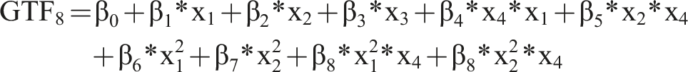
A theory is an abstract entity of generalizable and testable explanations for a phenomenon’s observable and measurable gestalt—its ground truth—and forms the basis for predictions on the future gestalt of the phenomenon (Gregor, 2006; Popper, 2002). Theories aim to explain why phenomena have the observed gestalt and how phenomena will change depending on varying related factors (Lindberg, 2020). CTD approaches require identifying parts of the mathematical functions that define observed ground truths (Zhang et al., 2022)—the GTFs. Considering the complex nexus of environmental factors, social actors, and artifacts, as is characteristic of IS phenomena (Yoo, 2010), capturing all relevant variables and relations perfectly in a dataset is highly unlikely. Thus, datasets contain fractures and incomplete versions of GTFs (Fisher et al., 2019; Gregor, 2006). ML can identify parts of these fractures of GTFs through prediction models (Shmueli and Koppius, 2011; Shrestha et al., 2021). However, the patterns captured in the predictive models are correlative in nature (Smith, 2020) and the mere patterns themselves do not directly offer theoretical insights (Berente et al., 2019). To transform patterns into theory requires abductive reasoning, that is, finding a plausible explanation for the observed patterns through human sensemaking (Behfar and Okhuysen, 2018; Lindberg, 2020; Miranda et al., 2022a).
Through abductive reasoning, researchers can critically evaluate ML-detected patterns and provide explanations for why the observed patterns exist in such a manner (Behfar and Okhuysen, 2018; Lindberg, 2020; Shrestha et al., 2021; Zhang et al., 2022). Thus, they pursue explanatory approaches that illuminate the mechanisms causing the relationships in the data (Zhang et al., 2022). To this end, they assess the observed patterns to determine whether variables plausibly reflect causal relationships (Lindberg, 2020; Shrestha et al., 2021; Zhao and Hastie, 2021) or whether they are not helpful for theorizing, for example, because they could be spurious patterns resulting from measurement errors or random correlations (Smith, 2020). Further, plausible variable relations need to be expanded through abstraction on a substantive and terminological level (Berente et al., 2019) to benefit a theoretical understanding of a given phenomenon. Abductively developed theoretical explanations, grounded in the ML analysis of empirical data, allow researchers to generate hypotheses (Behfar and Okhuysen, 2018; Lindberg, 2020; Shrestha et al., 2021) and feed into the discussion of the theoretical insights in a research field through lexical integration (Berente et al., 2019). Therefore, patterns can initiate and inspire abductive approaches to theorizing and provide a basis for empirical testing; however, discovered patterns must not be mistaken for empirical validation themselves (Zhang et al., 2022). Patterns and predictions are not theory (Sutton and Staw, 1995), but they can offer new insights that inspire theory and that might have been missed without ML.
Interpreting black-box ML patterns—A shortcoming in extant CTD application studies and guidelines
CTD using ML is a very promising research field, although researchers currently receive only context-specific guidance rather than generalizable advice. To offer broader, actionable insights applicable across various contexts requires a comprehensive framework.
Extant studies on CTD applications show how valuable combinations of computational or ML methods and abductive theorizing can be used to build new theories. Lindberg et al. (2022) utilized Variable Length Markov Chains to analyze sequences of ideas and problem-related information in online ideation contests recorded as digital traces, identifying patterns that precede high-quality ideas. To explain the observed patterns, they iteratively compared them to creative cognition literature, based on which they eventually formulated a theoretical model to explain how information contributed after a prior idea had impacted the quality of subsequent ideas. Miranda et al. (2022b) employed Latent Dirichlet Allocation to analyze 4,925 blockchain-related texts, identifying prevalent topics across seven discursive fields and using Multidimensional Scaling to illustrate topic relationships. This methodological approach allowed for uncovering previously unknown patterns across fragmented blockchain discourses. These computational patterns were integrated with qualitative analyses and iteratively refined to form a theory linking identified topics to broader concepts of framing diversity and coherence in innovation discourse. Their study revealed distinct mechanisms for enactment fields, where coherence was managed conventionally, and for mediated fields, which acted as bridges between fields, promoting discourse coherence even as diversity increased. Also, their study highlighted that innovation discourses from different discursive fields coevolve as they echo each other. Tidhar and Eisenhardt (2020) analyzed 66,652 Apple Store products to investigate business models and optimal revenue strategies, combining Exploratory Data Analysis, multiple-case theory building, and ML, using algorithms such as Random Forest. They identified patterns such as the prevalence of freemium models among popular products and developed a theory explaining how revenue models capture value by aligning with user activities in the value creation process thereby exemplifying how predictive ML and traditional theory development methods can be combined to add value in fields with vast accessible data.
However, since the aforementioned studies apply CTD rather than aiming primarily to offer methodological guidelines, they provide limited actionable advice for CTD beyond their specific cases. Two papers specifically address this shortcoming for CTD researchers by providing actionable advice for CTD. First, Zhang et al. (2022) propose a context-specific five-step framework for theorizing organizational routines using computational sequence analysis to detect patterns through frequent subsequence mining and clustering analysis. They employ retroductive 3 reasoning to disclose generative mechanisms and validate these through empirical corroboration and triangulation, emphasizing human explanation to transform patterns into theory. Through combining a critical realist view with computational pattern detection, they pave the way for innovative accounts of changing organizational routines. Second, Shrestha et al. (2021) present a broader approach, explicitly building on predictive ML for theory building. They outline a four-step process of splitting data into samples for pattern detection and validation, using ML for pattern detection, applying abductive reasoning to build theories, and testing hypotheses deductively with traditional methods. The authors encourage researchers to utilize ML and large quantitative datasets to identify robust patterns, which then serve as the foundation for subsequent abductive theory development.
While the aforementioned studies provide initial guidelines for applying CTD and highlight its research value, they do not address the crucial issue of the interpretability of the computational approaches and the patterns they reveal. Despite interpretability, that is, the degree to which humans can understand patterns identified in ML models (Dhurandhar et al., 2017; Lee et al., 2024), being a pivotal concern in applying ML effectively for CTD (Shmueli and Koppius, 2011; Shrestha et al., 2021; Zhang et al., 2022), this concept is rarely discussed in the corresponding literature. Either these studies do not address interpretability explicitly (Lindberg et al., 2022; Miranda et al., 2022b), or they label it as important without substantially elaborating its relevance for theory construction (Shrestha et al., 2021; Tidhar and Eisenhardt, 2020; Zhang et al., 2022). Potentially, ML algorithms can create black-box models that are characterized by opaqueness and overwhelming complexity, which inhibits human interpretation of the identified patterns (Du et al., 2020; Guidotti et al., 2018; Gunning et al., 2019; Rudin, 2019). Without further analyses, such lacking interpretability prevents using those black-box models in CTD approaches. However, separate explanation approaches that approximate the inherently non-interpretable patterns through XAI (Barredo Arrieta et al., 2020; Gunning et al., 2019; Rudin, 2019) enable human interpretation of these patterns, thus potentially facilitating the use of black-box models in CTD.
Although algorithms creating effective black-box models, such as Neural Networks (Zhang et al., 2022) or the XAI approaches that illuminate the ingrained patterns, have been rejected for CTD without a detailed examination (Shrestha et al., 2021), many have relied on algorithms that create inherently interpretable models—so-called glass-box models (Rudin, 2019; Zhang et al., 2022). Using glass-box ML models for pattern detection in CTD seems to be an obvious choice, because their inherently transparent nature enables understanding the particular ML model (Fisher et al., 2019; Guidotti et al., 2018; Gunning et al., 2019). In such a setting, humans can interpret the entailed variables, their impact, and possibly even their interaction effects (Shrestha et al., 2021). However, for some tasks, black-box models can be superior 4 (Asatiani et al., 2021; Kim et al., 2023) and include previously unknown relations (Jiménez-Luna et al., 2020; Webel et al., 2020). Therefore, especially when knowledge of the data and the studied phenomena is limited, while the ML selection and the formulation of expected structures of patterns 5 in data is complicated, using a black-box model together with XAI can be a sensible choice (Kim et al., 2023). Generally rejecting black-box models leaves a gap in the CTD literature, thus hindering the rigorous integration of these models in CTD and limiting CTD’s potential to contribute to research.
Despite one notable exception (Choudhury et al., 2021) initially contributing to this gap, the remaining void in the literature is remarkable. Choudhury et al. (2021) offer some initial guidelines for using an XAI approach (Partial Dependence Plots) for interpreting black-box ML models. They briefly discuss the opportunity to use the ML-detected patterns that have been made interpretable for inductive or abductive theorizing. However, their study does neither discuss the capabilities and shortcomings of XAI for the suggested use, nor how to implement the identified patterns in an abductive theorizing process. The absence of these explicit considerations of theorizing and the suitability of XAI leave questions on how and to which extent XAI can fruitfully be used in pattern detection for theorizing, thus preventing researchers from considering the combined use of black-box ML models and XAI for CTD.
SHAP as XAI tool in harnessing black-box ML potential for theory development
Various methods, referred to as (post-hoc) XAI (Barredo Arrieta et al., 2020; Gunning et al., 2019; Zacharias et al., 2022), have been suggested to reveal the patterns in black-box ML models, to achieve some degree of interpretability (Barredo Arrieta et al., 2020; Zhao and Hastie, 2021). XAI approaches can be classified according to different characteristics, regarding model specific or model agnostic explanation type, the global or local level of explanation, and method of representing an explanation (Barredo Arrieta et al., 2020; Xie et al., 2023). The resulting explanations can be represented in various forms, including textual explanations, visual explanations, variable relevance explanations, and variable attribution explanations (Barredo Arrieta et al., 2020; Senoner et al., 2022). Model-specific XAI methods such as the embedded variable importance function of tree-based models (e.g., XGBoost) (Du et al.,2020) are limited in their applicability to these very models (Ribeiro et al., 2016). Contrarily, model-agnostic approaches (Ribeiro et al., 2016) can be used independently of model type (Du et al., 2020). While global explanations offer insight on the model-level, thereby explaining how the model as a whole reaches its predictions (Barredo Arrieta et al., 2020; Du et al., 2020), local explanations provide insight on the instance-level, that is, they reveal how variables impact the specific prediction for a single observation (Du et al., 2020; Zacharias et al., 2022).
Although we acknowledge the value of various XAI approaches for pattern detection (e.g., Barredo Arrieta et al., 2020; Choudhury et al., 2021), we suggest SHAP (Lundberg and Lee, 2017) as a particularly promising approach for CTD due to its statistically desirable characteristics 6 (Lundberg and Lee, 2017; Senoner et al., 2022), its versatility (Lundberg et al., 2020; Lundberg and Lee, 2017), and its widespread use in fields such as computer science and IS research (Bauer et al., 2023; Fernández-Loría et al., 2022; Gramegna and Giudici, 2021; Xie et al., 2023; Zacharias et al., 2022). SHAP is a model-agnostic approach and offers visual explanations of variable relevance and attribution for any kind of predictive model (Gramegna and Giudici, 2021) and provides insights on both global and local levels (Lundberg et al., 2020; Senoner et al., 2022; Zacharias et al., 2022). On a global model level, SHAP approximates which variables are the most important and how these variables impact the prediction (Lundberg and Lee, 2017). The results can also be shown graphically and are comparable across different prediction models, which enable pattern identification across different models. Additionally, SHAP can be used to reveal interactions between variables via an interaction plot (Lundberg et al., 2018; Zacharias et al., 2022). Overall, SHAP offers a versatile approach to reveal patterns across black-box ML models, making it particularly useful for a structured approach to CTD.
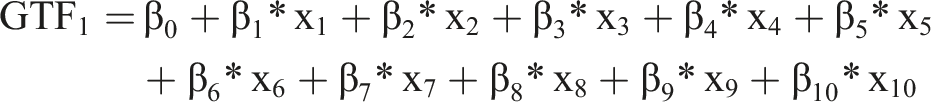
SHAP is a variable-additive approach, which builds a linear function g(z’) of binary variables to provide a prediction that approximatively matches the prediction of the original model f(x) built by the underlying ML algorithm (Kamath and Liu, 2021; Lundberg et al., 2018; Lundberg and Lee, 2017; Xie et al., 2023). The explanation model has the form
Originally developed for coalitional game theory to find a fair distribution of payouts for each player based on their respective contribution to the overall payout (Shapley, 1953; Zacharias et al., 2022), Shapley values indicate the contribution (fair payouts) of variables (players) to a specific predicted value (overall payout). These values were transferred to ML using SHAP values 7 (Lundberg and Lee, 2017). To exemplify the interpretation of SHAP values, consider the following binary classification situation: A black-box ML model predicts the turnover of IT-professionals (0 = turnover, 1 = no turnover) based on multiple variables (e.g., salary, paid overtime hours, tenure, and job satisfaction). A SHAP value can be computed for each variable, for instance, a monthly salary of USD 5,000 is assigned a SHAP value of 0.3 for a certain IT-professional. This value of the variable drives the prediction toward no turnover by 0.3, that is, it predicts no turnover in this specific instance more likely than not. To trace the final prediction, we need the SHAP values for the other variables in this instance. If positive SHAP values outweigh negative ones, the model predicts no turnover (1); otherwise, turnover is predicted (0).
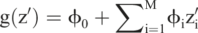
For CTD, however, local insights are less useful, and need to be transformed into global insights—the aggregated SHAP values of a variable across multiple instances Illustrative SHAP summary plot based on the prediction of a black-box ML model for nine variables.
8
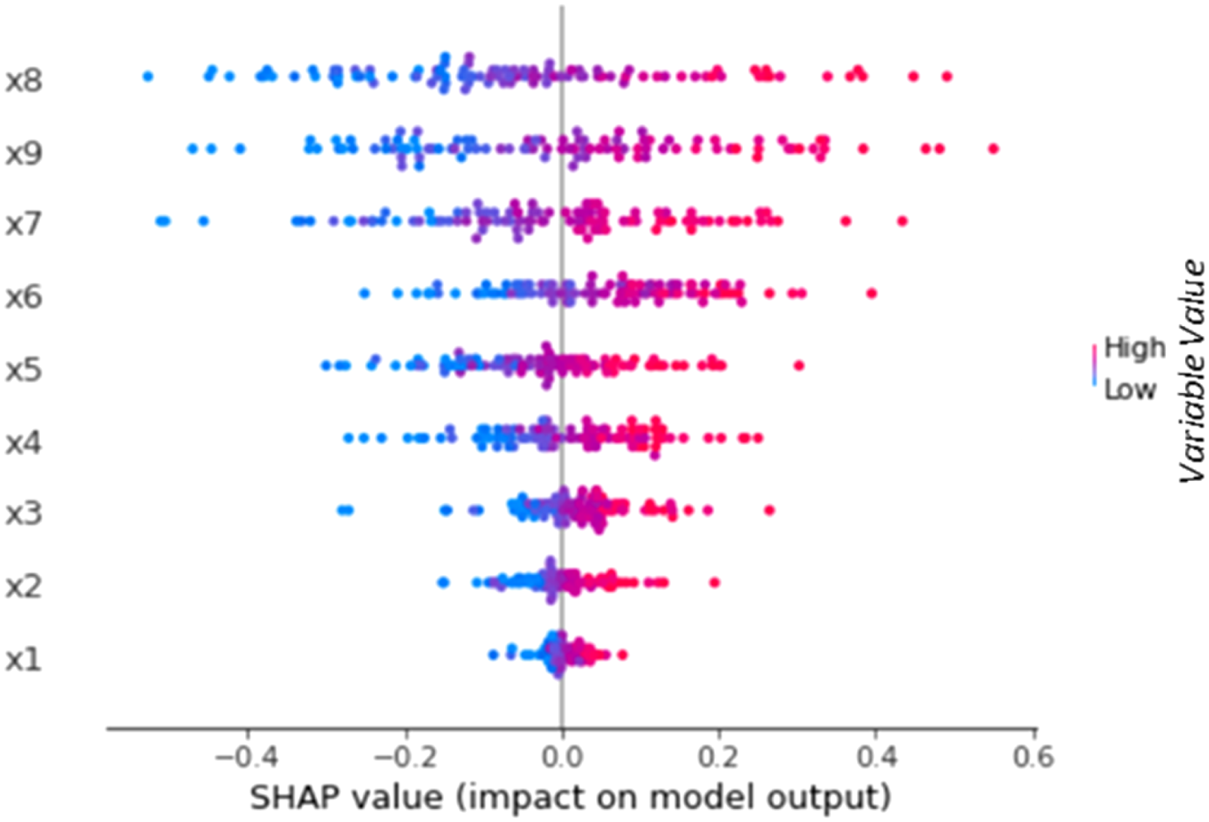
Further, dependence plots indicate the functional form of the relation between variables and the outcome prediction, and they can indicate interactions between variables in their impact (Lundberg et al., 2018). For this purpose, a variable’s SHAP values can be plotted against the variable’s values for the respective instances, indicating the functional form. Extending the plot by the course of the variable dependent on the value of another variable indicates interaction effects (see Figure 2 below for an example of both kinds of dependence plot). Interaction plots (left plot) indicate whether the impact of a certain variable (x6) depends on another variable (x7). Dependence plots can also be used to analyze the functional form of relations (right plot). Continuing the turnover example, we assume that paid overtime hours and tenure interact in a way that for IT professionals with high tenure, an increase in paid overtime hours lead to a lower likelihood of turnover prediction, as these employees may be more accustomed to longer work hours and thus appreciate the increased income more than they suffer from the additional workload. On the other hand, for IT professionals with low tenure, an increase in paid overtime hours could lead to a higher likelihood of turnover prediction, as they suffer more from the additional workload than they appreciate the increased income. Plotting the variable values of paid overtime hours against the SHAP values for this variable (in the left plot of Figure 2 this would correspond to x6) with respect to the variable value of tenure (x7 in the left plot in Figure 2) this would then show two crossing courses whereas high tenure values show a positive trend (red dots), and low tenure values show a negative trend (blue dots). Further, assuming that job satisfaction shows a nonlinear relation to turnover prediction, plotting this variable’s values against the SHAP values for this variable could show a course like the right plot in Figure 2 where x9 would correspond to job satisfaction. This plot would indicate that an increase in job satisfaction initially shows an increase in the SHAP values, indicating a higher likelihood of no turnover and could then level off at a certain point where further satisfaction does not significantly change the turnover prediction. Illustrative SHAP dependence plots based on the prediction of a black-box ML model for multiple variables.
9
Despite SHAP’s versatility in providing a broad range of insights into ML derived patterns, it has been criticized regarding the reliability of the ML derived interpretable patterns it discloses (Fernández-Loría et al., 2022; Xie et al., 2023). SHAP as post-hoc XAI faces general criticism for the inaccurate representations 10 of its separate explanation models generated to approximate the prediction model (Fernández-Loría et al., 2022; Gosiewska et al., 2021; Shrestha et al., 2021; Xie et al., 2023). All prediction models generated by ML algorithms are imperfect representations of the actual patterns that shape data or phenomena (Fisher et al., 2019; Gosiewska et al., 2021; Rudin, 2019; Shmueli, 2010; Shmueli and Koppius, 2011; Smith, 2020). Even models with high predictive performance across different datasets on a phenomenon represent only parts of the true relations shaping the phenomenon and can contain spurious patterns (Grisold et al., 2024; Smith, 2020) or, to optimize predictive performance, omit relevant relations (Shmueli, 2010). To allow for interpretability, these patterns are presented in a simplified way, for example, through lists or visualizations of low dimensionality (Barredo Arrieta et al., 2020). This carries the risk of these patterns being oversimplified, which further lowers an XAI approach’s fidelity to the original prediction model (Gosiewska et al., 2021). Arguing that XAI methods are potentially oversimplified and generally deliver imprecise representations (Gosiewska et al., 2021; Rudin, 2019; Rudin et al., 2022) of “wrong” original models (Fisher et al., 2019), some have rejected XAI for CTD in general (Shrestha et al., 2021).
Besides the general criticism and rejection of XAI, some initial steps have been made to examine SHAP’s limitations. Slack et al. (2020) illustrated SHAP’s vulnerability to adversarial attacks, that is, to the deliberate modification of input data in ways imperceptible to users, aiming to produce intentionally misleading explanations (Bauer et al., 2023; Senoner et al., 2022). Further, Fernández-Loría et al. (2022) show that SHAP produces inconsistent results across multiple runs if a high number of variables is included in an analysis. That is, in explaining a prediction at the local level, using many variables can yield different variables as the most important ones to explain an outcome, or may indicate different importance weights when analyzed multiple times. Also, their analyses indicate that SHAP can obscure each variable’s individual impact on an outcome by averaging out the positive and negative impacts variables have in the presence of nonlinearities and interaction effects between variables (Fernández-Loría et al., 2022). Considering the general criticism of XAI and the particular limitations SHAP exhibits, one has to acknowledge that patterns detected using SHAP are imperfect and, depending on the context, can even be misleading.
However, imperfect patterns are not inherently useless (Fisher et al., 2019) as long as the models provide meaningful, even if incomplete, insights in the phenomenon represented in that data (Grisold et al., 2024; Shrestha et al., 2021). Considering the complexity of real-world phenomena, it is highly unlikely that data on a phenomenon would replicate it in a perfect model 11 even if there were statistical approaches to find that model (Gregor, 2006; Grisold et al., 2024). Theories simplify the complex reality to present an interpretation (Gregor, 2006); thus, the imperfection of SHAP insights does not prevent theory development as long as we can confidentially assume that the identified patterns can capture substantial aspects of the patterns which ML models detected. If we know the circumstances in which inferences from XAI patterns can safely be made, we can use it as confidently as other statistical and non-statistical methods of pattern detection. To the best of our knowledge, there is no in-depth investigation of these circumstances for SHAP in the context of CTD. Addressing this gap, we simulate data on phenomena with predefined IS-like GTFs and investigate indications that SHAP can confidently be used for pattern detection in CTD.
Study I: Simulation analysis to evaluate the reliability of SHAP’s GTF representations
Set-up of the simulation
To evaluate the reliability of SHAP’s representations of actual patterns in the data, we must compare SHAP’s output with these actual patterns. In real-world data, the entirety of patterns that actually define an observable ground truth remains (partially) unknown (Grisold et al., 2024), which limits the assessment of ML and XAI methods (Shrestha et al., 2021). Therefore, we generate self-defined GTFs as mathematical functions. Knowing the GTFs allows us to directly compare the SHAP output to actual patterns in the GTFs and, thus, to evaluate the reliability with which SHAP is able to capture these patterns. We implemented GTFs of different complexity which we base on theoretical models analyzed in multiple recent IS studies. Additionally, we manipulated our data with some common shortcomings, to resemble the varying complexity and imperfection of real-world datasets (Choudhury et al., 2021; Shrestha et al., 2021). To ensure reliable results, we use a Monte Carlo simulation approach (Chin et al., 2003; Kock and Hadaya, 2018; Peng et al., 2023; Thies et al., 2018), generating 1,000 datasets, and calculate the individual labels based on the defined GTFs. In total, we train 96,000 ML models using six different ML algorithms, eight different GTFs, and two error term variants: one with random error and one with systematic error. Based on these trained ML models, we calculate the SHAP values to analyze the reliability of SHAP’s GTF representations in terms of (1) identification of relevant variables, (2) identification of dependency direction and shape, and (3) identification of interactions between the relevant variables.
Development of GTFs as basis for the comparison
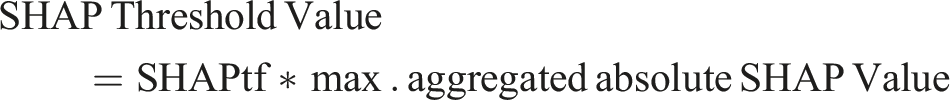
As basis for our analysis, we use several GTFs that resemble functions known from IS research and related disciplines. Using these GTFs, we know the precise form of F(x) and, therefore, how the input variables (X) generate the output (Y). Additionally, to render the GTFs more realistic, we add noise and an error term to the GTF.
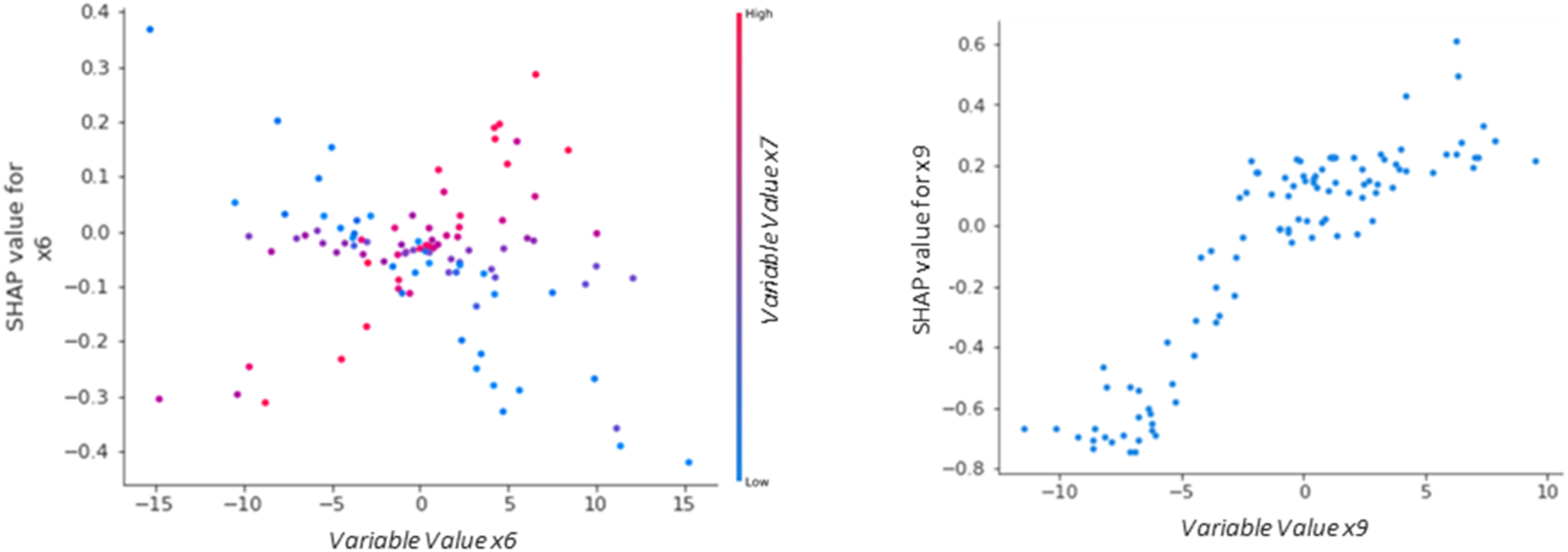
As baseline, we use
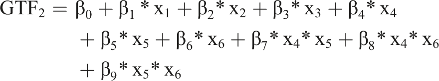


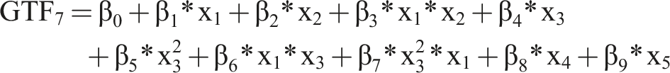

For all GTFs, we chose the values of
Since we define the problem as a binary classification problem, we assigned each instance of the dataset to a class according to whether the output of the GTF was above or below a certain threshold value. We generated 1,000 simulated datasets for the GTFs, comparable to the sample size used in other IS studies (Chin et al., 2003; Kock and Hadaya, 2018; Peng et al., 2023; Thies et al., 2018). We assumed a normal distribution for the individual variables, with a mean of 0 and a standard deviation of 1 (Shrestha et al., 2021). Additionally, we randomly varied the number of instances of the datasets between 200 and 2,000 and randomly added non-relevant variables, so that we had 10–20 variables for each dataset. On average, each dataset contained 15.7 variables, resulting in an average of non-relevant variables of 9.3 across the different GTFs. Based on these input variables, we created the ground truth labels based on our eight GTFs with two different error terms (systematic and random).
Training of ML models and calculating the SHAP values
To compare different results and to demonstrate the reliability of SHAP’s GTF representations based on different models, several ML models should be included in the analysis. To reach high performing ML models through training requires several steps (e.g., Choudhury et al., 2021). Finally, the predictive performance of an ML model can be evaluated by using different metrics and the SHAP values can be calculated based on the trained ML models.
Even for experienced data scientists, determining the best-fitting ML model a priori is hardly possible (Choudhury et al., 2021; Tidhar and Eisenhardt, 2020). Thus, we applied a range of frequently used glass-box and black-box models as is common in ML analysis (Choudhury et al., 2021). We incorporated common black-box models such as Artificial Neural Network (ANN) (Hassoun, 1995), Random Forest (RF) (Breiman, 2001), Support Vector Machine (SVM) (Cortes and Vapnik, 1995), as well as common glass-box models such as Logistic Regression (LR) (Hosmer et al., 2013), Decision Tree (DT) (Breiman et al., 1984), and K nearest neighbors (KNN) (Kotsiantis et al., 2006).
Due to the data being synthetic, there was no need to perform any further data quality checks or data cleansing. We split the dataset into a test dataset and a training dataset (Choudhury et al., 2021), using 80% of the data as training data and 20% as test data (Kim et al., 2023; Rácz et al., 2021). The ML model’s predictive performance can be evaluated with the accuracy, which is a common metric for ML models 12 (Choudhury et al., 2021). The accuracy is measured using the test data to indicate how many of the instances are classified correctly.
For the post-hoc analysis of the ML models we used SHAP due to its popularity, versatility, and ease of interpreting outputs (as elaborated above) (Gramegna and Giudici, 2021). To calculate the SHAP values, we used a sample of the entire dataset to provide a comprehensive and representative set of SHAP values 13 (e.g., Li, 2022; Meng et al., 2021; Mokhtari et al., 2019).
Analysis
We conducted the sub-analyses by (1) identifying the relevant variables, (2) identifying the relevant variables’ dependency direction (e.g., positive or negative relation between variable and SHAP values) and shape of dependency (e.g., u-shaped or linear), and (3) identifying interactions between the relevant variables.
Analysis 1: Identifying the relevant variables
The aim of this analysis is to obtain the relevant variables from the GTFs while excluding non-relevant variables. SHAP only provides an importance ranking which does not indicate whether the variables are actually relevant (Fernández-Loría et al., 2022; Molnar, 2020), that is, part of the GTF. This raises the question as to which SHAP value should be the cut-off point for a variable to be identified as relevant. To investigate this, we tested under different conditions how the chosen cut-off point of the SHAP value impacts the identification of correct variables and the number of identified variables. This aims to check whether we have identified all the relevant variables in the GTF.
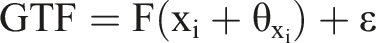
For this purpose, we need a SHAP threshold value as a boundary, which determines how many variables are considered relevant and, hence, used for theorizing. To calculate the SHAP threshold value, we use a SHAP threshold factor (SHAPtf), which is a relative factor of the highest aggregated (absolute) SHAP value of a variable. An increase in the SHAPtf results in a higher SHAP threshold value and thus a more restrictive selection of variables, and vice versa. We use the SHAPtf because the optimal relative level of the SHAP threshold value is unknown, necessitating testing various levels to identify the most appropriate threshold for variable relevance. For example, if we choose the SHAPtf as 20% and the maximum SHAP value is 10, then the SHAP threshold value is 2 (0.2*10). In contrast to a fixed threshold value or an average-based approach, the SHAP threshold value offers adaptability to the model and data. The maximum SHAP value, thus the SHAP threshold value, adjusts automatically to the specific model, dataset, and used parameters (e.g., sample size for the SHAP values). Also, the alternative use of a threshold value based on the average value has the disadvantage of being influenced by the overall distribution of SHAP values (e.g., by a high number of non-relevant variables). Therefore, a threshold based on a factor of the maximum absolute aggregated SHAP value will most likely better reflect the actual relevance of the variables in the context of the specific model, data, and other circumstances.
14
Further we defined the ratio of correctly identified variables, as the sum of all correctly detected variables (i.e., relevant variables) divided by the sum of all detected variables (relevant and non-relevant variables).
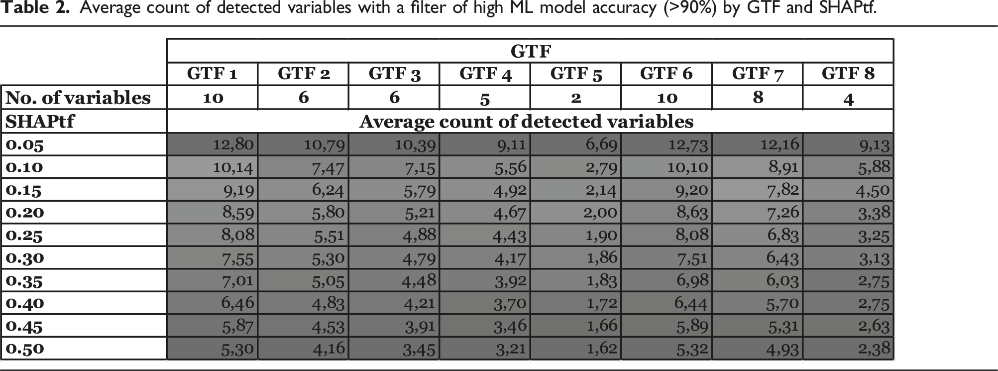
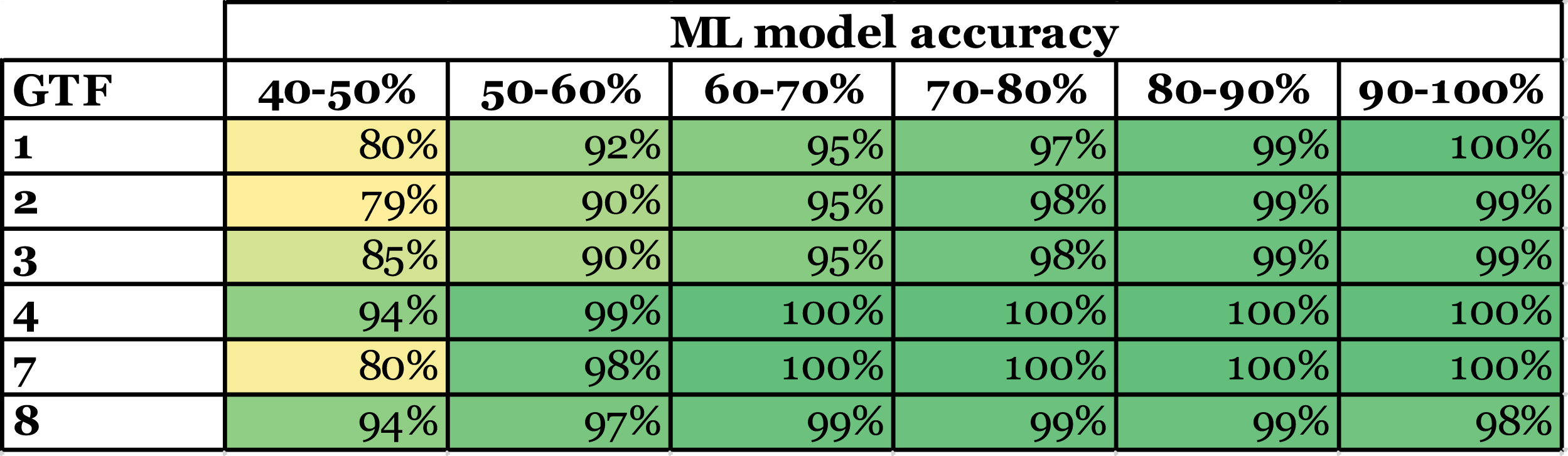
Using the SHAPtf and the ratio of correctly identified variables, we examined the reliability of SHAP’s GTF representations. We have analyzed how various simulated conditions, such as dataset size, GTF structure, the magnitude of error terms, and the ML model predictive performance, impact the ratio of correctly identified variables when setting different SHAPtf. For instance, we investigated how the ML model accuracy influences the ratio of correctly identified variables, specifically whether a higher ML model accuracy leads to a higher ratio of correctly identified variables at the same SHAPtf. Ratio of correctly identified variables sorted by SHAPtf and ML model accuracy.
15
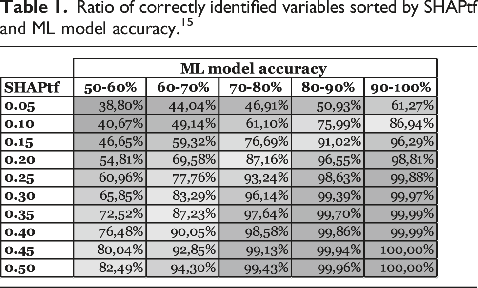
The analyzed factors impact the ratio of correctly identified variables if we set the SHAPtf equally. In particular, for large datasets (with over 1,500 instances) the ratio of correctly identified variables is 90%, while for small datasets (under 500 instances) the ratio of correctly identified variables is 79% (for a SHAPtf of 0.25). The structure of the GTF has an even bigger influence. For GTF1 the ratio of correctly identified variables, on average, is 97%, for GTF5 only 65% (again for a SHAPtf of 0.25). A smaller factor on the average ratio of correctly identified variables has the standard distribution of the noise term at roughly 7% difference for different settings. In real-world cases, we do not know the structure of the GTF and, at best, have only limited knowledge of the individual noise and error terms’ magnitude. However, these factors very likely influence the ML model’s predictive performance (e.g., in terms of accuracy) (Choudhury et al., 2021; Hastie et al., 2009) and, consequently, the ratio of correctly identified variables.
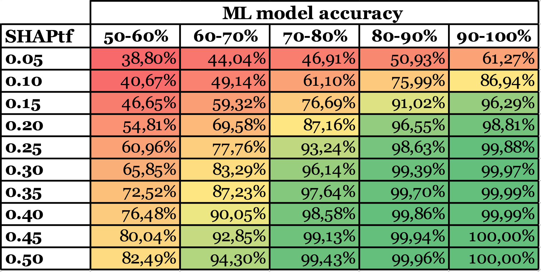
Average count of detected variables with a filter of high ML model accuracy (>90%) by GTF and SHAPtf.
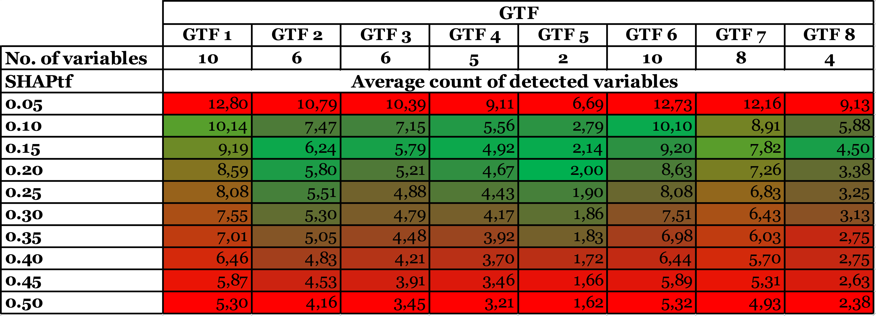
This reveals a trade-off between detecting relevant variables and reliability in the variables detected, where a SHAPtf between 0.10 and 0.15 appears to offer well-balanced results in terms of the number of identified variables (Table 2). It typically identifies most of the truly relevant variables while minimizing the exclusion of potentially relevant ones. This range provides a good compromise between inclusivity and selectivity, both crucial for reliable pattern detection in CTD. However, to ensure that the identified variables with this SHAPtf are correct with high confidence, the achieved model accuracy should be considered (see Table 1).
Figure 3 summarizes this trade-off. In the “adequate” case, we set a high SHAPtf. This leads to mainly correctly detected variables but would also filter out relevant variables of the GTF. This approach should be used if the ML model accuracy is low. It helps to identify the relevant variables (though not necessarily all) while avoiding the incorrect identification of non-relevant variables, which would be the “poor” case. The “superior” case would be to have a high ML model accuracy and a SHAPtf set low to thereby detect all relevant variables of the GTF without identifying non-relevant variables.
The trade-off between SHAPtf and ML model accuracy reflects the relationship between a model’s predictive performance and SHAP’s ability to reliably identify relevant variables. Models with higher predictive performance permit a lower SHAPtf, enabling confident identification of more variables as relevant. This relationship is pivotal in CTD, guiding researchers in assessing the level of complexity their models can reliably capture for theory development.
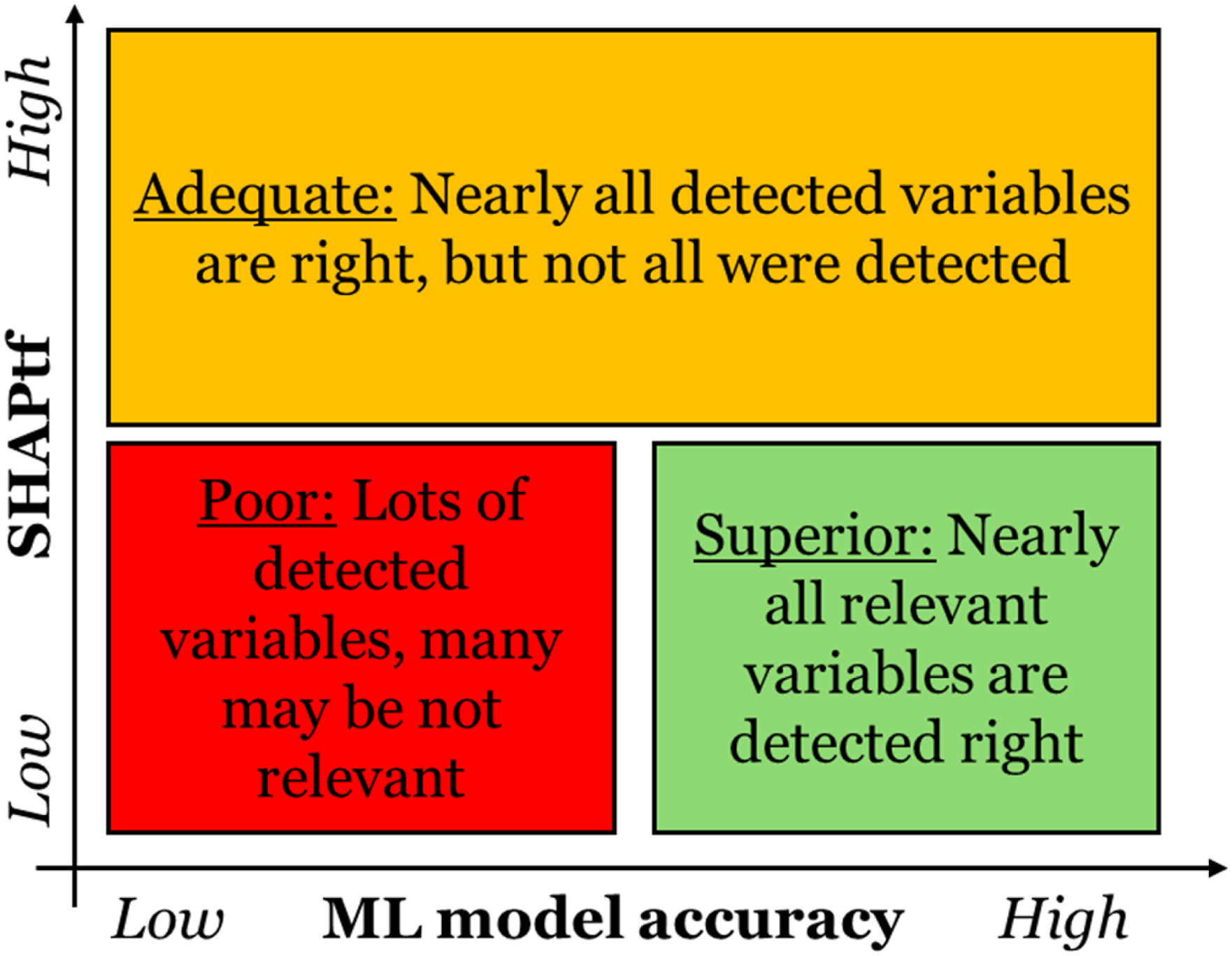
Connection between the SHAPtf and the ML model accuracy.
Analysis 2: Identifying the variables’ dependencies
Once we have identified the relevant variables, the next question is in which direction these variables affect the prediction. Since the signs in our GTFs can be both positive and negative, the direction of the effect should ideally match these signs. For this purpose, we created a correlation factor between the variable value and the respective SHAP values. With a positive beta value, we expect a positive correlation factor and vice versa.
To determine the reliable representation of the GTF in this aspect, we measure the correct dependency direction rate, which ultimately indicates the percentage of correctly detected dependencies.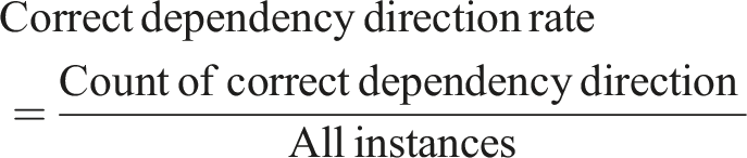
Correct dependency direction rate by GTF and ML model accuracy.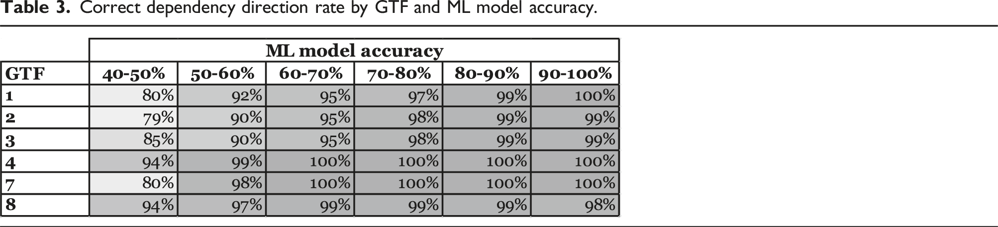
We see that an ML model accuracy of 60%–70% identifies a correct dependency direction in at least 95% of all cases, while 80%–90% ML model accuracy identifies a correct dependency direction in at least 99%. Overall, the SHAP representation of the direction of dependency appears to be very stable even with lower accuracy of the ML model and, therefore, also for different circumstances (i.e., data and GTF).
A more detailed analysis allows us to derive the shape of the dependency by plotting the SHAP values against the respective variable values. This can indicate linear and polynomial dependencies, as is illustrated in Figure 4. The variables in GTFs with polynomial terms exhibit a u-shape in contrast to the true linear curves. The direction depends on whether the beta value is positive or negative. Therefore, the dependence plot of the relevant variables should be analyzed additionally, to determine whether it is a linear or other-shaped one.
However, when a variable appears in several terms of the GTF with both positive and negative beta values, the relationship between the variable’s value and the SHAP value becomes less clear. The trend is dominated by the heights of the betas, so we can only make statements about the aggregated influence of the variable.
In the case of interaction terms in the GTF, the picture becomes increasingly diffuse, as their dependence plots exhibit no dominant trend, since the SHAP values also depend on other variables. This requires a fine-grained analysis of potential interaction effects between the variables, which we present in Analysis 3.
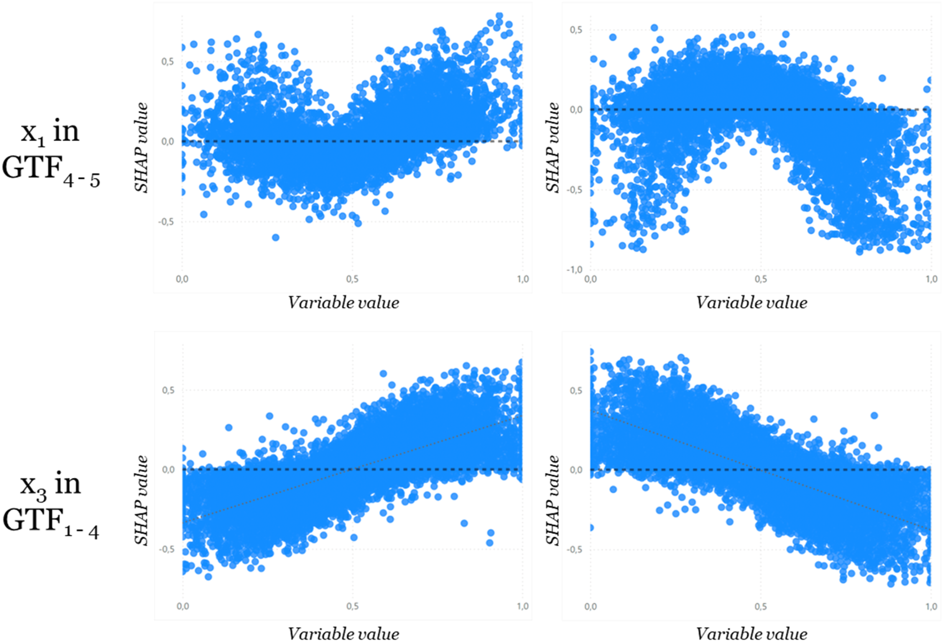
Dependency of variable x1 for GTF4–5 in comparison to x3 for GTF1–4 with ML models >60% accuracy and positive (left) and negative (right) beta.
Analysis 3: Identifying the interaction effects
Finally, we looked at the interactions by plotting the bivariate interactions among the most relevant variables. As discussed in Analysis 2, to identify more complex behavior of the relevant variables requires additional analyses. To detect interaction effects, the relevant variables can be plotted against each other. This approach should always be considered if the dependence plots of the variables are fuzzy or unclear, because this is an initial indication of more complex relationships.
We illustratively assessed the interaction of variable x4 with variable x6 in GTF2,3. Without the effect of variable x6 Interaction of variable x4 with x6. Additionally, the lower/higher value of variable x6 is indicated by the color scheme (dark blue – low; light blue – high).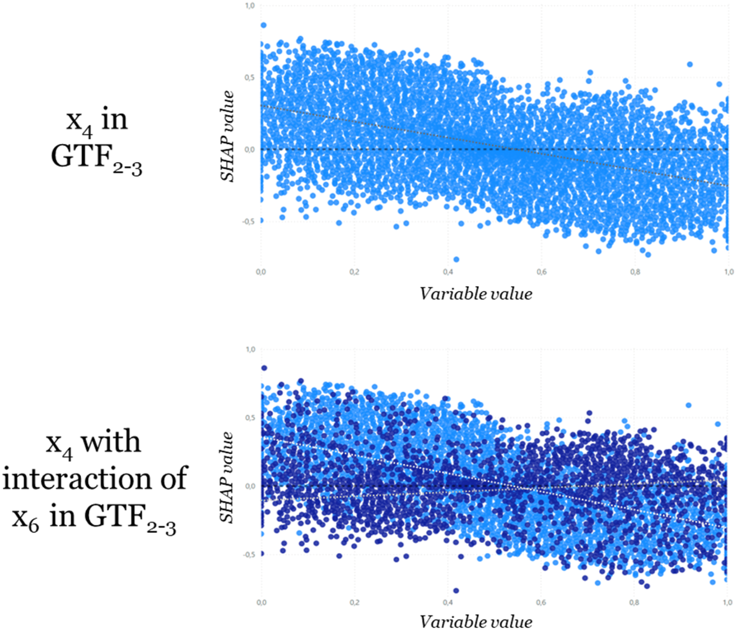
In contrast, without interaction terms (e.g., for variables in GTF1) we do not recognize a similar separation for variables, which shows that linear terms on average do not show an interaction effect.
In summary, study 1 demonstrates that the SHAPtf approach provides a flexible and reliable method for identifying relevant variables in SHAP outputs. There is a clear trade-off between ML model accuracy and the SHAPtf required for reliable variable identification. Researchers can use this trade-off to gauge the complexity of patterns they can confidently extract from the models. Also, our findings indicate reliable detection of the dependency direction of relevant variables, even at moderate levels of ML model accuracy. This approach enables the use of black-box models for pattern detection in CTD while maintaining methodological rigor.
Study 2: Using SHAP for CTD in a real-world case
In our approach using SHAP, patterns are not a substitute for theory; they show what is observed, rather than explaining why something is observed (Sutton and Staw, 1995; Zhang et al., 2022). Although data and patterns can serve to build theory, researchers are required to be explicit on how they develop theories from the data (Weick, 1995) using computational methods as building blocks (Berente et al., 2019; Lindberg, 2020; Miranda et al., 2022a). We illustrate this by showing potential steps for delineating patterns the XAI analyses disclose and provide suggestions for subsequent theorizing.
Before any theorizing, the CTD approach needs to be structured and defined regarding both content and available data. Particularly, knowing the relevant literature is helpful in identifying a research gap and developing a (preliminary) research question (Gehman et al., 2018). To build theory from data using computationally intensive methods, researchers can benefit from a range of well-established methodologies (Berente et al., 2019). Yet for CTD, the process requires gathering data of sufficient complexity to record insightful observations (Berente et al., 2019). Additionally, extant datasets on a phenomenon might already be available, even if not previously subjected to computationally intensive approaches, thus containing still undiscovered insights.
Step 1: Assess initial data on a relevant phenomenon
In our example, we were intrigued by the question of why digital service quality varies substantially across similar means of transportation, especially in airline travel. An initial literature review revealed considerable research interest in the topic in the 2000s; even so, we could not find a satisfactory explanation. We found this interesting because improving airline passengers’ service experience could be particularly relevant in this highly competitive market (Bubalo and Gaggero, 2015; Carlton et al., 2019). While a variety of papers in this stream incorporated measures of technology experience or proficiency, digital service experiences were particularly related to self-service technology (Feng et al., 2019; Lee et al., 2012; Makarem et al., 2009). With limited insight thus far, it seemed important to interrogate the phenomenon in order to illustrate our methodological application. 16 Instead of collecting primary data through observation, we identified an existing real-world “Passenger Airline Satisfaction” dataset 17 (Hayadi et al., 2021). This dataset provided a record potentially relevant to the phenomenon we are investigating. Based on 23 input variables (see Appendix C), such as satisfaction level of different services (e.g., online boarding), individual characteristics (e.g., age), or departure delay, and 123,880 instances we explain why passengers are satisfied or not (satisfied = 1; neutral or not satisfied = 0), particularly focusing on the role of digital service elements.
Step 2: Pre-select models and prepare the dataset for analysis
Prior to any methodological application, researchers should assess their data regarding data quality and adequate model selection. We assessed the quality of the airline dataset and applied data transformation when necessary, as in dealing with, for example, missing information and outliers (García et al., 2015; Kotsiantis et al., 2006). Particularly, we re-coded nominal variables into dummy variables (one-hot encoding) and aligned min–max scaling of metrical variables to correct for unnecessarily divergent variable ranges (Hancock and Khoshgoftaar, 2020; Nayak et al., 2014). Further, based on our research goal and the dataset, we chose an appropriate ML approach to conduct a classification analysis and to determine whether customers tended to show above average satisfaction. It is hardly possible to predict in advance which ML model would have the best predictive performance (Choudhury et al., 2021). Thus, we applied the same ML models as in our validation study, that is, we used ANN, RF, SVM, LR, DT, and KNN, applying the predefined hyperparameters of the ML models of the scikit-learn library (Pedregosa et al., 2011). Subsequently, we divided the dataset into training and test data, with 80% being used as training data (Rácz et al., 2021).
Step 3: Evaluate predictive performance and determine the SHAPtf
We proceeded to analyze the resulting models with particular attention to predictive performance, using accuracy 18 as metric to ensure that potentially relevant models’ quality was satisfactory for harnessing insights. In our case, all models excepting the LR showed an accuracy exceeding 92% (accuracy across models: LR 0.873; DT 0.945; KNN 0.927; SVM 0.946; MLP 0.960). 19 We then compared the models directly and selected the best performing model—RF with an accuracy of 0.962—for further analysis with SHAP. In line with our previous analysis, it could offer insight on the underlying phenomenon and allowed us to choose a lower SHAPtf for variable identification. To calculate the SHAP values, we relied on a random subsample of the dataset. This approach yielded consistent results while optimizing computational resources to a manageable level.
Step 4: Identify the relevant variables
In line with our approach outlined in the simulation study and based on the model accuracy, we selected the relevant variables based on their relative SHAP value. In particular, we employed a SHAPtf of 0.20 relative to the maximum SHAP values displayed for any variable. Building on our previous analyses, this combination of model accuracy and SHAPtf could be expected to display the variables accurately with a probability of 98.81% (see also Tables 1 and 2). Choosing a lower SHAPtf would most likely mean incorporating additional yet irrelevant variables, particularly for a SHAPtf below 0.15. Choosing a higher and more restrictive SHAPtf would lead to fewer identified relevant variables, possibly excluding relevant variables while providing only incremental additional confidence in the identified variables.
Based on the SHAP summary plot, we also derive the distinct aggregated SHAP values. Since inflight wifi service is the most important variable (with an aggregated SHAP value of 284.08), we determine the SHAP threshold value to be 56.82 (0.2 * 284.08). In Appendix D, we display all SHAP values of the variables and the selection of those variables with aggregated SHAP values above 56.82.
Applying the aforementioned SHAPtf yielded a total of 11 variables (Figure 6) that could offer insight relevant to customer satisfaction and also entailed two variables (inflight wifi service and online boarding) that explicitly corresponded to internet or online services. SHAP summary plot of RF for real-world example of passenger satisfaction.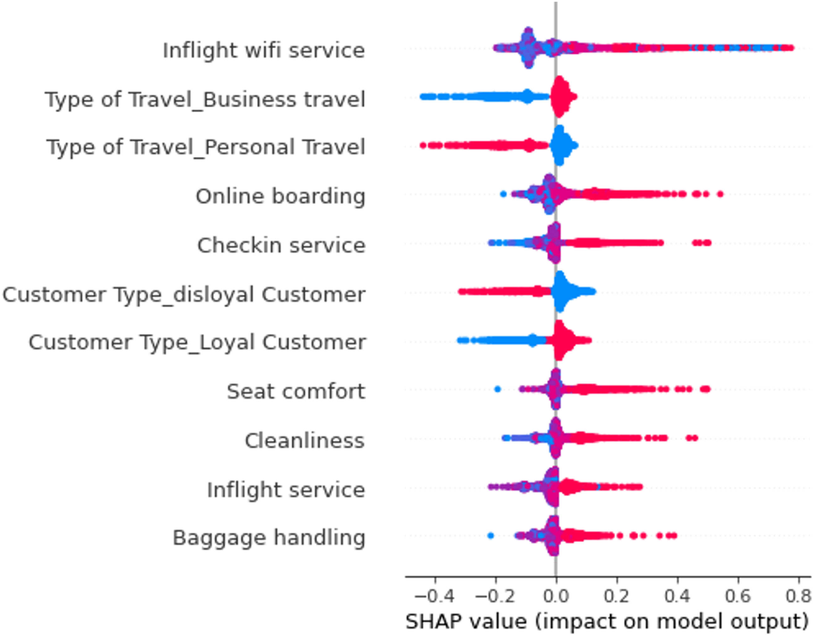
Step 5: Identify the direction and form of the variable impact
To gain further insight on how different variables impact our prediction, we turned to the SHAP dependence plots to analyze the relationship between the variables and their SHAP values (Lundberg et al., 2018). The variables’ corresponding SHAP values for the predicted satisfaction could offer indicators as to whether a given variable continuously and systematically impacts satisfaction (e.g., low variable values link to lower satisfaction, while high variable values link to higher satisfaction) or whether the impact is selective (e.g., only low variable values link to low satisfaction while high variable values show no clear link to satisfaction). The 11 variables showed the following patterns:
SHAP dependence plot for the variable inflight wifi service.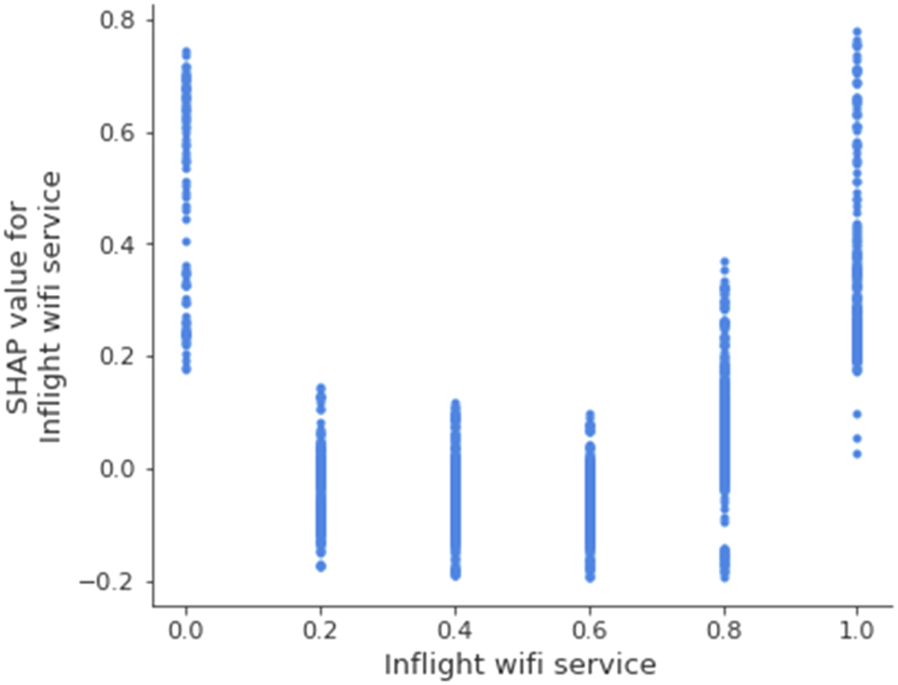
SHAP dependence plot for the variable online boarding.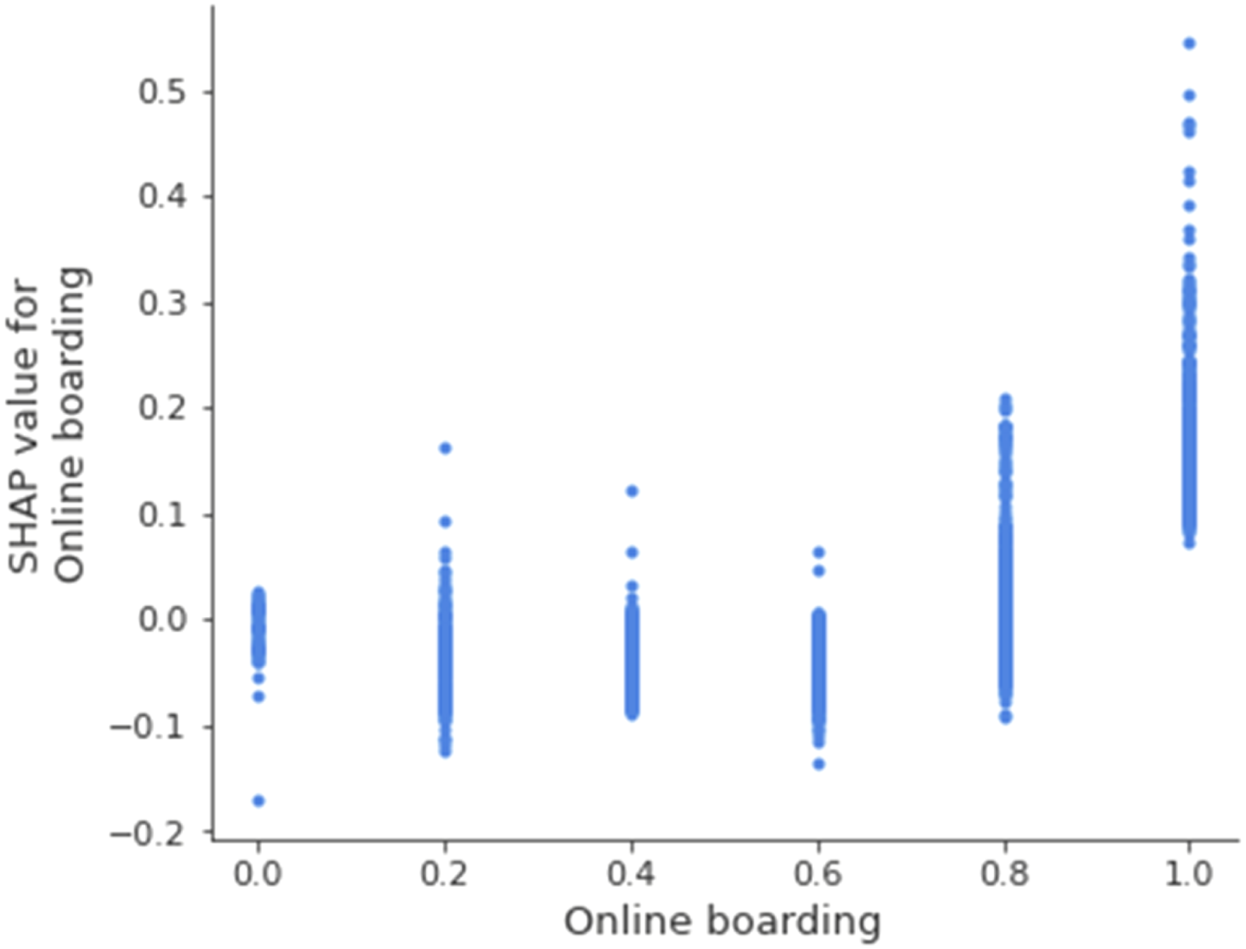
SHAP dependence plot for the variable checkin service.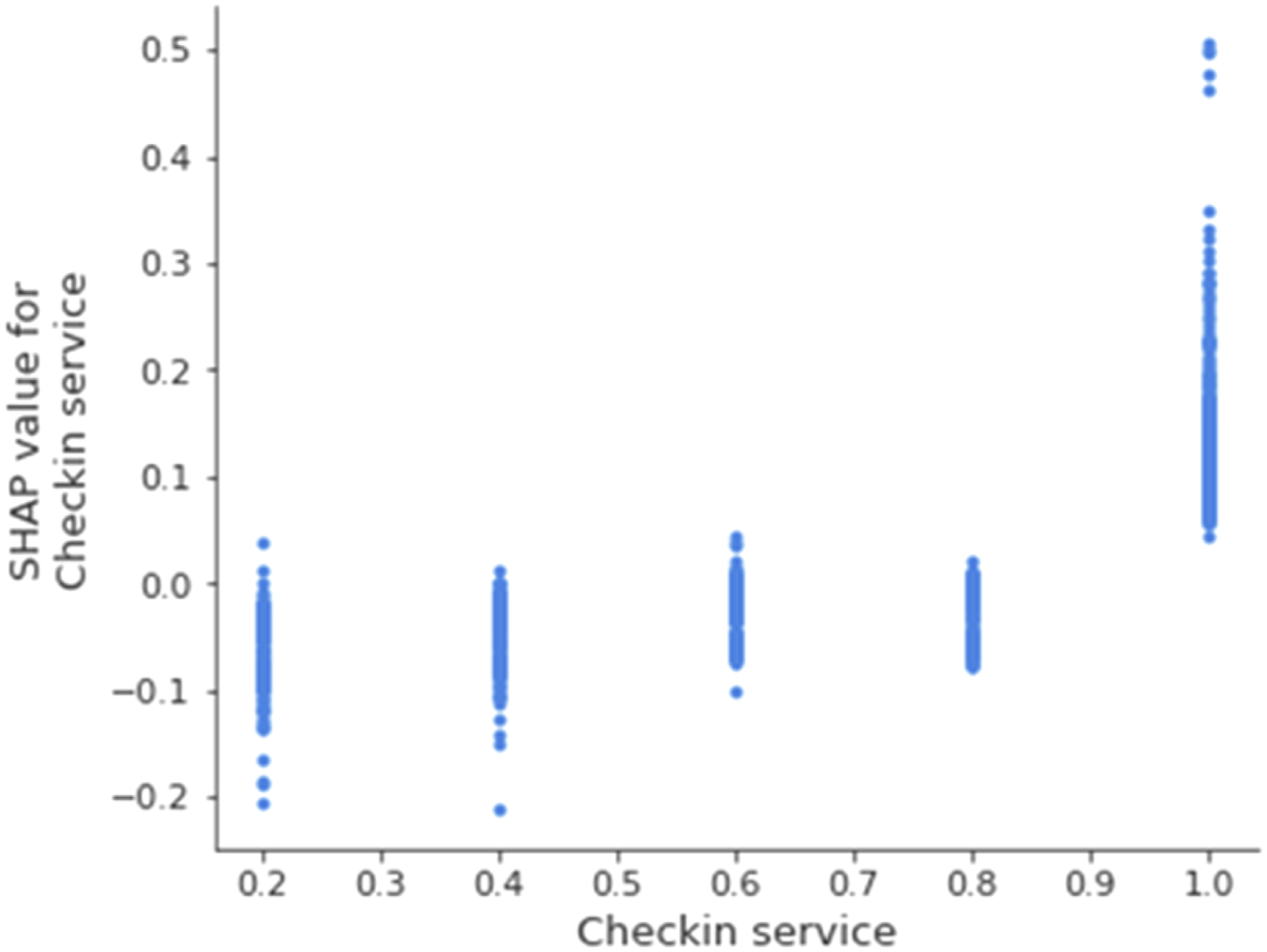
SHAP dependence plot for the variable seat comfort.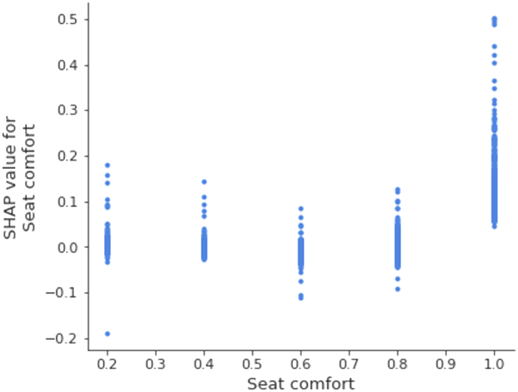
Using the dependence plots and analyzing the SHAP values we gained additional insight on the predictive pattern, as the plots reveal how distinct variable expressions link to the resulting prediction. For example, one should not assume that inflight wifi service always benefits customer satisfaction, since the pattern suggests that low wifi quality reduces the predicted satisfaction. Across continuous variables, tendentially low or average rating corresponded with slightly negative average SHAP values. From the direct variable effects, we conclude that only exceptionally positive perceptions of services impacted satisfaction positively. Consequently, explaining satisfaction is not about performing rather well across variables; rather, it is about excelling in the relevant ones—most of all in inflight wifi service.
Step 6: Identify potential variable interactions
Next, we plotted SHAP dependence plots with interactions for the relevant variables previously identified. This would deliver additional insights into potential interaction effects, particularly for the relevant variables where we observed a high variance of SHAP values in the single characteristics, indicating a possible interaction. Essentially, these plots could hint at how an interaction of variables amplifies their effects on the predicted outcome. Overall, plotting the interaction of SHAP values did not provide a very clear picture for most variables. Only the interaction of inflight wifi service and online boarding showed a peculiar relationship (Figure 11). While the absence of inflight wifi service impacted the prediction positively, this effect was reduced if customers ranked the online boarding service highly. Further, where low rated inflight wifi service was combined with high ranked online boarding service, the SHAP values slightly improved. Nevertheless, the impact on the prediction is small. Given this interaction, online boarding might have implications for the peculiar positive impact in cases where no wifi was available, but beyond that it provides hardly any additional insights. SHAP Interaction plot for the variable inflight wifi service with online boarding.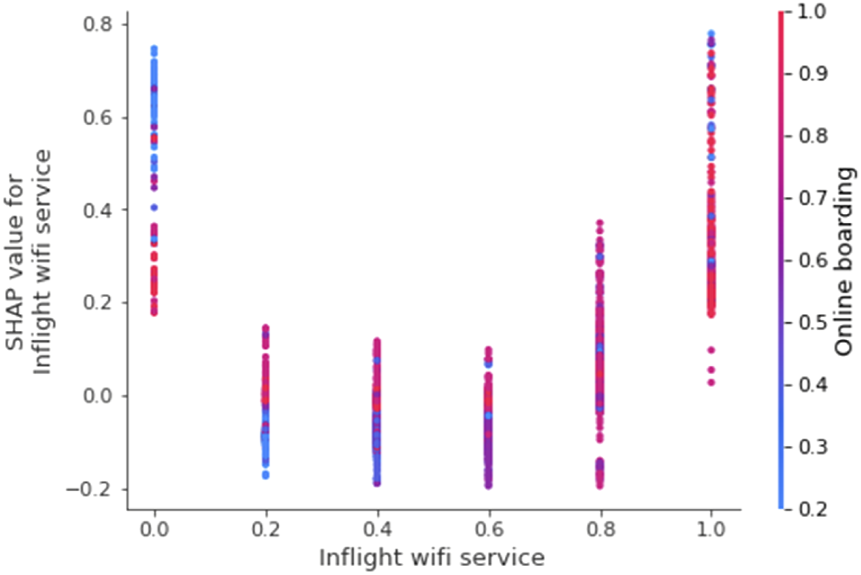
Step 7: Move beyond the patterns toward initial theorizing through abduction
In sum, the patterns disclosed in this illustrative example provided four interesting insights. First and foremost, the approach identified the most relevant variables for explaining satisfaction of airline customers. Strikingly, the digital services were highly relevant while physical services had lower impacts on the predictions. This inspired two possibly naive hypotheses stating that either customers find physical services to be of lesser importance per se, or physical services, compared to digital services, show less variance across airlines, and thus were less decisive regarding satisfaction ratings.
Second, the variable distributions highlighted the nonlinear impacts of services and particularly digital services (inflight wifi service satisfaction and online boarding satisfaction) on satisfaction. Essentially, only excellent ratings corresponded to positive average SHAP values. Thus, selectively offering exceptional service quality, particularly in digital services, had a greater positive impact on customer satisfaction than an overall above average, yet not optimal, evaluation. Satisfaction in the prediction model is a nonlinear relationship based on exceptional service experiences. Thus, service quality would be inaccurately represented if modeled as a linear regression in the given dataset.
Third, strikingly, for the variable inflight wifi service offering no service at all led to higher predictions of satisfaction than offering low or moderate inflight wifi services. This was surprising and again showed that given the prediction model, satisfaction was estimated best through selective variable values rather than aggregating linear variable relationships.
Last, the approach offered very few indicators for variable interactions, beyond the impact of the unavailability of wifi services in combination with excellent online boarding services. This interaction could be particularly interesting in further investigation of the peculiar positive impact of unavailable wifi but has limited impact on the global model for satisfaction.
Based on the SHAP insights, one could engage in initial abductive theorizing. Despite the importance of digital services, and especially of wifi services, being essentially important for satisfaction, these variables’ impact only shows when excellent services are provided. Any lower service quality does not provide a benefit and performs worse than cases in which no such service is provided. This all-or-nothing evaluation can be challenging to organizations as neither pilot-projects nor initial imperfect and small-scale projects may yield any immediate positive feedback, while they could potentially even create the opposite. Seeing no benefit from investments could in turn be interpreted as customers’ indifference regarding this kind of service, thus providing an argument against any further investment. Yet, the patterns in our data show the need to excel in providing an inflight wifi service if they are to reap benefits from customer satisfaction, since only optimal ratings were associated with positive SHAP values when wifi was available.
Building on the disclosed patterns, we engaged in abduction to benefit our theorizing. As neither data nor list of variables or diagrams are sufficient means of theory, we engaged specifically in abstracting, generalizing, and explaining (Weick, 1995) to develop a plausible description of our observations. We formulated preliminary hypotheses about our observations, such as “Airline customers will only report additional satisfaction if a service is excellent.” We then extrapolated the hypotheses to different contexts such as train travel and general public transportation to assess whether these still appeared plausible. Further, we tried to develop possible explanations for our observations, which we then challenged in extensive discussions, debating whether the explanations were sufficiently likely (Behfar and Okhuysen, 2018). We found the following example seemed plausible: From a methodological perspective, the u-shaped distribution can be missed when modeling linear effects for customer satisfaction and thus was not detected in extant research (Feng et al., 2019; Lee et al., 2012; Makarem et al., 2009). Given our approach, various models can be run to compete for an adequate representation of the data at hand and thereby essentially contrast different attempts in modeling the variables’ impacts on the predicted outcome. Thereby less intuitive distributions—such as the u-shaped impact of inflight wifi service—can emerge despite not explicitly tuning models to the underlying pattern.
From a substantive perspective, if providing high quality digital services requires substantial investment, organizations are likely to conduct feasibility and pilot studies prior to investing in large scale rollouts. However, assuming that pilot studies have substantial budget restrictions (as saving on unnecessary investments is a central underlying intention in pilot studies), the services provided will most likely not be of cutting-edge quality. At the same time, without wifi customers may turn to relaxing activities such as reading, watching an inflight movie or listening to music, instead of surfing or working, which is likely to be experienced as particularly cumbersome when the inflight wifi service is poor. Considering our data, any rudimentary service quality might not have any positive impact and thus benefit arguing against substantial investments.
Consequently, an underinvestment in wifi services could result from the poor evaluation of initial projects. Subsequently, further investment required to provide excellent wifi would be reduced. Thus, the generally poor service quality in public transportation (or the absence of a wifi service) could result from the described path dependence, rather than from customers’ lack of interest. Finally, we engaged in thought trials (Weick, 1989) challenging our explanation, asking whether we would still have expected an underinvestment if pilot studies had shown the decisive impact of inflight wifi service, and the answer is no. Would we have expected the results to persist given the progress in technology development and constant connectivity via personal devices? Here we answer yes, all the more because the personal device internet access could create a reference value for evaluating the wifi service. Through these and numerous additional challenges, we gained confidence in our preliminary explanation.
Iterating between these sensemaking procedures and the patterns, we returned to the SHAP output. Strikingly, we noted that the SHAP exploration of the prediction model widely approximated the satisfaction essentially by aggregating excellent ratings only. Based on this consistent pattern, researchers could additionally engage in theorizing the circumstances under which such patterns arise (only for complementary or even for core services) and the degree to which they are reflected in extant theoretical models. Thereby, researchers could ultimately refine existing theories along routes that would not have been discovered using linear conceptualizations. The final theoretical model can eventually form the basis for quantitative validation, using both different (and possibly more sophisticated) operationalizations of the measures and different, independent datasets.
Given the exploratory nature of our inquiry we urge careful assessment of any subsequent hypotheses. The patterns derived by SHAP only reflect the given data. Abductive theorizing and reflecting on the model’s plausibility in the light of extant literature will be decisive for effective theorizing and theoretical model development. The patterns do provide a starting point that could challenge existing theories or explanations. Building on the abductive theorizing approach, combining the patterns and insights from extant literature, hypotheses need to be formulated and tested (Shrestha et al., 2021) to ensure that emergent patterns prevail beyond a single case or dataset (Vaast et al., 2017). Any theorizing and abductively derived hypothesis need subsequently to hold up to the empirical validation in separate and explicitly sampled datasets, while using a rigorous quantitative methodology. This, however, exceeds the scope of our proposed framework for detecting patterns in black-box models.
Discussion
We started out with the question: How and under what circumstances can XAI, and particularly SHAP, be used to detect patterns for Computationally Intensive Theory Development? To answer this question, we employed an extensive simulation study to assess the capabilities of SHAP for pattern detection based on synthetic datasets modeled with varying GTFs. Subsequently, we demonstrated our approach using an exemplary application scenario.
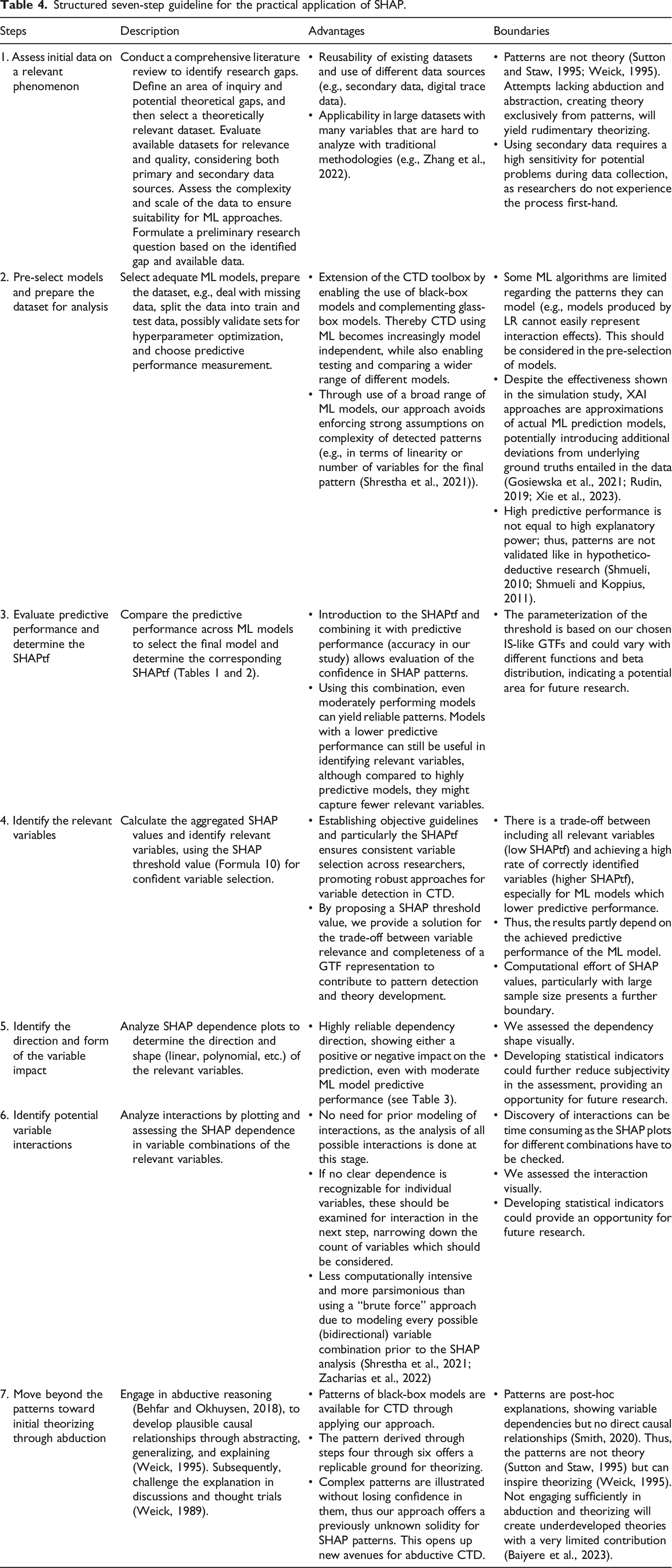
Structured seven-step guideline for the practical application of SHAP.
Contributions to literature
We offer three overarching contributions to literature: First, we extend extant guidelines for pattern detection and abductive theory development (Choudhury et al., 2021; Shrestha et al., 2021; Zhang et al., 2022) showing how SHAP and black-box models can be used effectively. Second, we guide the application of SHAP through a standardized and replicable seven-step guideline, contributing to the CTD toolkit (Berente et al., 2019; Lindberg, 2020; Miranda et al., 2022a) and next-gen theory development in IS (Burton-Jones et al., 2021; Grover and Lyytinen, 2023). Third, we contribute to the methodological discussion on XAI and SHAP in IS research, developing a metric for confident SHAP use (Fernández-Loría et al., 2022; Kim et al., 2023; Zacharias et al., 2022).
First, our study lays the foundation to enable using highly effective black-box ML models for CTD through SHAP. We provide evidence that SHAP can identify patterns accurately and with sufficient confidence. While some studies generally reject black-box ML models for CTD (Zhang et al., 2022) or are skeptical of XAI in CTD (Shrestha et al., 2021), our approach shows how SHAP can be used responsibly to harness the power of black-box models. Further, we add to the literature on ML and XAI application (Choudhury et al., 2021) by explicitly evaluating XAI for pattern detection and these patterns’ use as a basis for abductive reasoning. On the one hand, we demonstrate that SHAP, a commonly used XAI approach, produces highly reliable GTF representations and helps to capture central dimensions of patterns in data when two essential metrics are considered. On the other hand, we provide a step-by-step guide on how to combine ML and SHAP for pattern detection and CTD, detailing key considerations.
Our simulation study demonstrates that considering the predictive performance of an ML model and setting a threshold (SHAPtf) for SHAP values to determine variables’ relevance allows us to use SHAP for receiving reliable GTF representations. By taking these two factors into account, we can make warranted judgements about SHAP’s applicability in specific cases. Additionally, the trade-off between these factors offers guidance on the potential complexity of the derived patterns, indicating how many variables can be reliably considered for further analysis. By substantiating the circumstances under which SHAP can be used confidently, we support its rigorous use in CTD and show that black-box ML models can indeed add value to CTD (Shrestha et al., 2021; Zhang et al., 2022).
Our real-world example in study 2 demonstrates the practical application of our approach to CTD using SHAP. By applying this method to analyze an exemplary dataset, we show how it can uncover patterns that might be overlooked by traditional methods. Based on these insights, we have developed a seven-step guideline. This guideline provides instructions on how to use SHAP for pattern detection and how to apply these patterns to CTD (see Table 4). Following our guideline supports researchers in shedding light on different aspects of ML patterns through SHAP and identifying relevant variables and their impact, as well as potential interactions between variables. The emerging patterns can then be used as input in abductive reasoning from real-world data to theorize the constituting mechanisms and eventually formulate a theoretical explanation.
Nevertheless, using black-box ML models and SHAP together rigorously, demands that we consider some crucial points. On the one hand, an effective application requires sufficient data quality and a form that allows for ML and SHAP application. On the other hand, for an accurate application the applied methods themselves require profound knowledge and expertise in statistics, ML, and XAI. Furthermore, interpreting the resulting patterns requires expertise regarding the investigated phenomenon, as well as in theory development. Otherwise, one risks producing superficial or nonsensical theories (Baiyere et al., 2023) or might mistake mere patterns for theory (Sutton and Staw, 1995), while patterns only entail observations of empirical regularities without explaining why these regularities exist (Lindberg, 2020; Zhang et al., 2022). To use the described approach, we emphasize that authors need a diverse skillset individually or within the research team to effectively engage in CTD, as recent studies illustrate (Lindberg et al., 2022, 2024; Miranda et al., 2022b).
Yet, our approach does not transform black-box ML models into transparent glass-box-models (Gosiewska et al., 2021; Rudin, 2019; Xie et al., 2023); rather, it approximates the ML models. Thus, it is important to stress that the ML-identified patterns are still correlative in nature (Choudhury et al., 2021; Smith, 2020). Even if the underlying ML models reach high predictive performance, they can potentially still contain spurious patterns in the XAI output (Smith, 2020). SHAP does not perfectly capture the constituting patterns and adds a deviation, as any approximation would. Not knowing the GTFs in real-world data, leads to potentially unobservable deviations in patterns and XAI representations (Rudin, 2019; Rudin et al., 2022), which subsequently disconnects the abductive theorizing approach from the underlying real-world mechanisms (Zhang et al., 2022). However, we show that selecting the SHAPtf based on a model’s predictive performance can substantially increase confidence in the identified variables. By evaluating SHAP’s reliability in representing GTFs through the aforementioned trade-off, we take an initial step toward addressing the potential problem of misleading patterns. Having these boundaries in mind when using black-box ML models together with SHAP and combining these approaches with careful abductive reasoning, this combination offers a valuable extension for pattern detection in CTD.
Second, our standardized and replicable approach to using ML and SHAP as basis for abductive theorizing, contributes to the ongoing discussion on CTD (Berente et al., 2019; Lindberg, 2020; Miranda et al., 2022a) and on a larger scale to next-gen theory development in the IS field (Burton-Jones et al., 2021; Grover and Lyytinen, 2023). As SHAP outputs are comparable across ML models and can be applied to a broad range of research cases (Lundberg and Lee, 2017), they provide a reasonable basis for a standardized and replicable approach to pattern detection. Our actionable step-by-step procedure lays the basis for exploiting SHAP’s potential in this regard and introduces a standardized and transparent, yet flexible, approach that can easily be reproduced following our seven steps. When considering dataset characteristics, our approach can be used for quantitative secondary data, trace data, or self-collected data. Of course, the interpretation in the abductive step will differ substantially depending on the kind of data and the phenomenon under investigation, for example, secondary psychometric survey data versus digital traces of app-use. Again, this emphasizes that domain knowledge on an investigated phenomenon is imperative—which is, however, no different to any other theory development approach (Shmueli and Koppius, 2011). The characteristics of a dataset, such as number of instances, measurement errors, etc., influence the output quality of our approach by impacting the predictive performance of the used ML models. Yet, our combined measure of the SHAPtf and the predictive performance (accuracy in our study) accounts for these factors. The trade-off indicates how complex identified patterns can be, while still providing reliable representations of patterns entailed. In cases of lower predictive performance, we can increase the threshold to ensure that, although fewer variables are identified, they are most likely relevant and not merely artifacts of the ML model or SHAP. Limitations in data quality or scope limit our approach just as they would limit any other approach, but through our trade-off metric we account implicitly for these limitations.
Third, showing how a trade-off between the SHAPtf and a model’s predictive performance helps to produce reliable GTF representations, our study contributes methodologically to the discussion on XAI and SHAP in IS research (Fernández-Loría et al., 2022; Kim et al., 2023; Zacharias et al., 2022). Essentially, what we found is that this trade-off allows us to evaluate how confidently we can use SHAP outputs. In analyzing our simulation study, we noticed a relation between high predictive performance and a low SHAPtf, where a high predictive performance allows us to use a low SHAPtf to identify many correct variables, that is, a substantial share of the GTF in the data. For our GTFs, a SHAPtf ranging from 0.10 to 0.20 for a model accuracy (the applied predictive performance metric) of 90% to 70%, respectively, has proven to be particularly promising, ensuring that we could identify (almost) all relevant variables without including non-relevant ones in the final SHAP outputs. Our analysis also implied that even receiving models with lower accuracy, we could still secure detection of relevant variables by setting the SHAPtf higher. In that case, however, the absolute number of correctly identified variables decreased, overall decreasing the complexity of the pattern we could derive from SHAP. However, all the patterns we received reflected relevant parts of the GTF. This is a valuable contribution because there are currently no unified methodological guidelines on how to secure reliable SHAP outputs. Therefore, our approach directly aids researchers in SHAP application and provides a refinement in the ongoing methodological discourse on the value XAI, and SHAP in particular, hold for IS research (Fernández-Loría et al., 2022; Kim et al., 2023; Zacharias et al., 2022). Our study allows us to use SHAP more effectively in IS research generally and in CTD specifically, while our nuanced analysis advances the methodological debate beyond simply endorsing or outright rejecting XAI and SHAP use.
Overall, our approach offers an extension to the CTD toolbox, essentially providing what Shrestha et al. (2021) call a “meta-algorithm” and offering a versatile complement to extant guidelines on pattern detection for abductive theorizing (Choudhury et al., 2021; Shrestha et al., 2021; Zhang et al., 2022). Thereby, we enrich computational methodology for CTD (Berente et al., 2019; Lindberg, 2020; Miranda et al., 2022a) and contribute to developing research methodologies for next-gen theorizing in the age of artificial intelligence algorithms (Burton-Jones et al., 2021; Grover and Lyytinen, 2023).
Limitations and future research
Despite taking utmost care in conducting our research, it is important to recognize the generalizability limitations of our approach.
Given the infinite possibilities for GTFs in reality, there are parameters and distributions that will not resemble our GTFs at all, which therefore prevent the assessment of SHAP’s capabilities in cases beyond the complexity of our simulation analysis. We created a simulation study comprised of 96,000 explanation models across 1,000 randomly generated datasets, covering eight GTFs and two error settings, to reflect the empirical complexities encountered. Our analysis approximates known scenarios within the IS field, relying on simplified models that might not capture GTFs’ true complexity (Grisold et al., 2024). While we are confident that generating complex datasets with multiple variations of parameters (e.g., error strength, the number of instances and variables) gives a good indication of SHAP’s capabilities to detect reliable patterns, this test is nevertheless not universally valid. Future research could extend our simulation approach to GTFs that resemble phenomena investigated in other research domains and that differ substantially in representing phenomena.
Additionally, we limited our approach to a binary classification problem not investigating multiple category classifications or a continuous predicted outcome variable. However, SHAP explanations can be used for such problems as well. Therefore, another extension to our approach could be to analyze non-binary classification problems and regressions problems, which could potentially lead to adoptions of our approach. For instance, for regression there are other predictive performance metrics, such as Root Mean Squared Error (RMSE) or Mean Absolute Error (MAE) (Kamath and Liu, 2021), that need to be considered for the confidence trade-off. Further, only certain ML models can be used for regression. This means some of our models can also be used for regression (e.g., RF, ANN, SVM, DT), while others need to be replaced (e.g., linear regression instead of logistic regression). The outputs of the SHAP plots are very similar, except that they do not show the contribution to the prediction of a specific class, but rather the relation to the specific output value. However, precisely evaluating and suggesting adoptions that needed to use SHAP for regression cannot be conclusively assessed on the basis of our study. This could be investigated further, for instance, using a comparable Monte-Carlo simulation approach as we did.
In the current approach, we assessed the form of the dependency between the variables and a predicted outcome as well as interactions only according to a visual assessment. Importantly, we chose the variables investigated visually based on a reliable and objective criterion as illustrated in the simulation study. However, this opens opportunities for further refinement in future research to use or derive quantitative criteria for the reliability of dependency and interaction. Also, examining the direct detection of interactions without investigating a large number of SHAP plots would further enrich our approach. SHAP offers some additional functions, such as the Interaction Index (Lundberg et al., 2018; Zacharias et al., 2022), that could be evaluated similarly to our approach using a simulation study.
Further, concept drifts—fundamental changes in phenomena, and thus in the data over time (Webb et al., 2016)—pose a substantial challenge to all approaches using ML for pattern detection. Concept drifts can significantly impact the predictions of ML models since patterns might not persist outside the initial dataset (Liu et al., 2024; Lu et al., 2019; Widmer and Kubat, 1996), thus leading to inaccurate predictions and to potentially unreliable and eventually useless XAI explanations. Concept drifts occur, for example, when different individuals enter an existing market or if natural disasters fundamentally change contextual factors (Liu et al., 2024). Consequently, concept drifts can impair theory development and particularly validation of XAI patterns. Therefore, researchers applying our approach need to consider potential concept drifts in their data, such as temporal or seasonal patterns, emergent changes to sample composition, or exogenous shocks. While concept drifts do not hinder our approach per se, they amplify the challenge for testing any ML pattern inspired theory.
Lastly, using black-box models and XAI limits troubleshooting. Although we have shown that SHAP can offer reliable representations of GTFs, the black-box ML models themselves remain opaque (Rudin, 2019). Consequently, in cases of ambiguous SHAP output, it is not clear whether this is grounded in the data, the ML algorithm or the resulting model, or whether it is due to SHAP. The drawback of using importance weights to indicate how a variable indicates decisions as well high computation time in comparison to other XAI approaches like counterfactual explanations (Fernández-Loría et al., 2022), is a further possible weak spot. Like Fernández-Loría et al. (2022), we see that complex interaction settings in combination with contrary beta signs in the GTF can limit the use of SHAP. Additionally, ML is generally challenged due to the risk of rising spurious patterns (Smith, 2020). Spurious patterns can emerge due to various factors, including issues in data collection, statistical anomalies (Bokelmann and Lessmann, 2019), overfitting in ML models (Choudhury et al., 2021), and sampling bias. Non-representative samples, in particular, can result in misleading patterns that offer little toward improved understanding of a phenomenon (Hastie et al., 2009).
Our approach inspires theory; it does not build it from XAI. However, the methodological challenges will potentially increase the challenge of validating these theories. We see an opportunity in re-testing patterns across datasets and contrasting instances of empirical validation from black-box and glass-box models to gain further insight toward advancing not only theory but also methodological development. To continually improve the validity of the insights we gain through ML and XAI for CTD, we need further research on such systematic sources of erroneous insight in patterns.
Conclusion
We set out to answer how XAI can be used to detect patterns for CTD, focusing on SHAP as a specific XAI approach. In a simulation study, we addressed the question under what circumstances SHAP can be used confidently to provide reliable results. Showing the trade-off between the predictive performance of the underlying ML model and the SHAPtf, SHAP offered reliable representations of patterns in data for IS-like GTFs. By revealing the combinations in which this trade-off promises reliable SHAP results, we contribute to a confident and rigorous use of SHAP for CTD. Further, we provide a seven-step guideline based on an illustrative application of SHAP in pattern detection as input to abductive theorizing. These two-fold insights contribute to using SHAP and, therefore, also highly effective black-box ML models for pattern detection in CTD, which ultimately contributes to the discussions on CTD, XAI in IS research, and next-gen theorizing in IS.
Footnotes
Acknowledgments
We would like to acknowledge that, as non-native speakers, we utilized AI assistance to check for and correct any grammar issues in our manuscript. Additionally, we took recommendations from AI on how to address the identified grammar and language issues.
Declaration of conflicting interests
The author(s) declared no potential conflicts of interest with respect to the research, authorship, and/or publication of this article.
Funding
The author(s) received no financial support for the research, authorship, and/or publication of this article.
Notes
Appendix
Author biographies