Discuss practical importance of results based on interval estimates and p -value functions,not only on point estimates and null p -values

Abstract

It has long been argued that we need to consider much more than an observed point estimate and a p-value to understand statistical results. One of the most persistent misconceptions about p-values is that they are necessarily calculated assuming a null hypothesis of no effect is true. Instead, p-values can and should be calculated for multiple hypothesized values for the effect size. For example, a p-value function allows us to visualize results continuously by examining how the p-value varies as we move across possible effect sizes. For more focused discussions, a 95% confidence interval shows the subset of possible effect sizes that have p-values larger than 0.05 as calculated from the same data and the same background statistical assumptions. In this sense a confidence interval can be taken as showing the effect sizes that are most compatible with the data, given the assumptions, and thus may be better termed a compatibility interval. The question that should then be asked is whether any or all of the effect sizes within the interval are substantial enough to be of practical importance.

Sen et al. (2022) advise looking at the practical importance of an effect estimate, keeping in mind its uncertainty, rather than only describing results as ‘statistically significant’ or ‘non-significant’. We applaud this and many of their other recommendations, for example that single p-values should be given with sensible precision and not be degraded to stars, letters, or binary inequalities (‘p < 0.05’) and that we should avoid using the phrase ‘statistically significant’ entirely. All of this is consistent with over 70 years of calls by many statistical writers to emphasize interval estimates over statistical tests (e.g. Altman et al., 2000; Cox, 1958; Cumming, 2012; McShane et al., 2019; Rothman, 1978; Rozeboom, 1960; Wasserstein and Lazar 2016; Yates, 1951; Yates and Healy, 1964). It is thus alarming that most papers screened by Sen et al. (2022) did not report interval estimates. Nonetheless, while we agree in broad terms with Sen et al. (2022), we think they do not go far enough regarding the following issues.

A single p-value for the null hypothesis of no effect is not enough

Sen et al. (2022) advise that both practical importance of an observed effect as well as its ‘statistical significance’ should be considered, where ‘significance’ seems to mean that the p-value is low. In their paragraph headed ‘Recommendations’, Sen et al. (2022) further advise using p-values to test the default null hypothesis of no effect. We think this approach is far from sufficient for analysis and reporting. We view the practice of testing only the null hypothesis of no effect as a manifestation of a cognitive and procedural bias called ‘nullism’, in which excessive focus is made on a ‘no-effect’ hypothesis at the expense of analysing reasonable alternatives as well. It has been argued that nullism is a pervasive source of distorted scientific reporting (Greenland, 2017), and we see it as a problem remaining in the Sen et al. (2022) article.

For example, their first recommendation includes a statement that ‘p-values are needed to help assess the extent to which chance might explain the results’, and they close their recommendations saying that ‘p-values are often helpful for ascertaining whether the reported effects of a treatment or explanatory variable can be attributed to sampling error’. To the extent that these recommendations are taken as referring only to p-values for the null hypothesis of no effect, they are misleading. One reason is that this no-effect p-value is calculated assuming that there is no effect and no uncontrolled sources of variation; we thus assume that any observed association (non-null effect estimate) is fully explained by chance alone (sampling error), and the same p-value cannot be used to ‘assess the extent to which chance might explain the results’. We fear the quoted recommendations invite readers to misinterpret the null p-value as the probability of the null hypothesis, which is a pure logical error and can be very misleading in practice (see misinterpretation no. 2 discussed in Greenland et al., 2016).

The need to shift interpretation towards compatibility

A large p-value for the null hypothesis of no effect only says that ‘pure chance’ is among the many hypotheses that are most compatible with the data, given the other statistical assumptions used to compute the p-value. Compatibility is an old concept in statistics (Bayarri and Berger, 2000; Box, 1980; Rothman, 1978), which has also been called consonance (Folks, 1981) and consistency (Cox, 1977) between the data and a hypothesis or model. In that literature, an observed p-value is a measure of compatibility (or consonance or consistency) between the observed data and a tested hypothesis, given a set of statistical assumptions (such as linearity and normality) which we will call the background model. To validly ‘assess the extent to which chance might explain the results’, it is necessary to present p-values for alternative hypotheses, along with the p-value for the null hypothesis that ‘the effect under study is absent and any observed association is from chance alone’. In other words, we need to use the same data to calculate p-values for multiple hypotheses, not just for the hypothesis of no effect, and to present those p-values side by side.

Researchers using confidence intervals already have the means for doing so. This is because a 95% confidence interval shows all hypotheses (possible values for the true effect size) that would get p > 0.05 and would thus not be ‘rejected’ at the 0.05 level when tested using the data and background model (Amrhein et al., 2019a, 2019b; Cox and Hinkley, 1974, Ch: 7; Greenland et al., 2016). The 95% interval thus shows the effect sizes most compatible with our data, given the background model. The interval shows that if a null hypothesis of no effect has p > 0.05 and is thus included in the interval, this inclusion only means that it is one of the many hypotheses (effect sizes) that are reasonably compatible with our data when using a 0.05 cutoff for ‘reasonable’, given the statistical assumptions.

Unless the point estimate has a value exactly corresponding to no effect, the hypothesis of no effect (and thus that any observed association is pure random error) is not the hypothesis that is most compatible with our data. Any other hypothesis with a larger p-value would be more compatible with the same data given the same background model. We can see this by plotting the p-values of all hypotheses in a compatibility graph or p-value function (also known as a confidence distribution or consonance curve; Berner and Amrhein, 2022; Birnbaum, 1961; Cox, 1958; Infanger and Schmidt-Trucksäss, 2019; Poole, 1987; Rafi and Greenland, 2020; Rothman et al., 2008, Ch: 10).

Figure 1 gives an example taken from Rafi and Greenland (2020) in which the effect measure is a hazard ratio (HR, the x-axis) in a proportional-hazards model; the p-values for different HR values are plotted on the y-axis. The graph visualizes possible values for the true effect size that are most compatible with the study data, given the background model. The 95% CI (compatibility interval, equals the classical ‘confidence’ interval) includes the null hypothesis of no effect (a hazard ratio of 1), which is just barely contained in the interval; the interval also covers hazard ratios of high practical importance (up to almost a 160% increase in hazard). The compatibility graph shows that most of those hypothesized values are more compatible with the data than the no-effect hypothesis because the p-values for those hypotheses are larger. The HR value most compatible with the data is the maximum likelihood (point) estimate of HR = 1.61.

Figure 1.

Compatibility graph or p-value function for hypotheses about how much a treatment of pregnant women with serotonergic antidepressants increases the hazard rate of autism-spectrum disorder in their children. The data are from Brown et al. (2017) and the plot is taken from Rafi and Greenland (2020); for more information on the plot, see the main text and Rafi and Greenland (2020).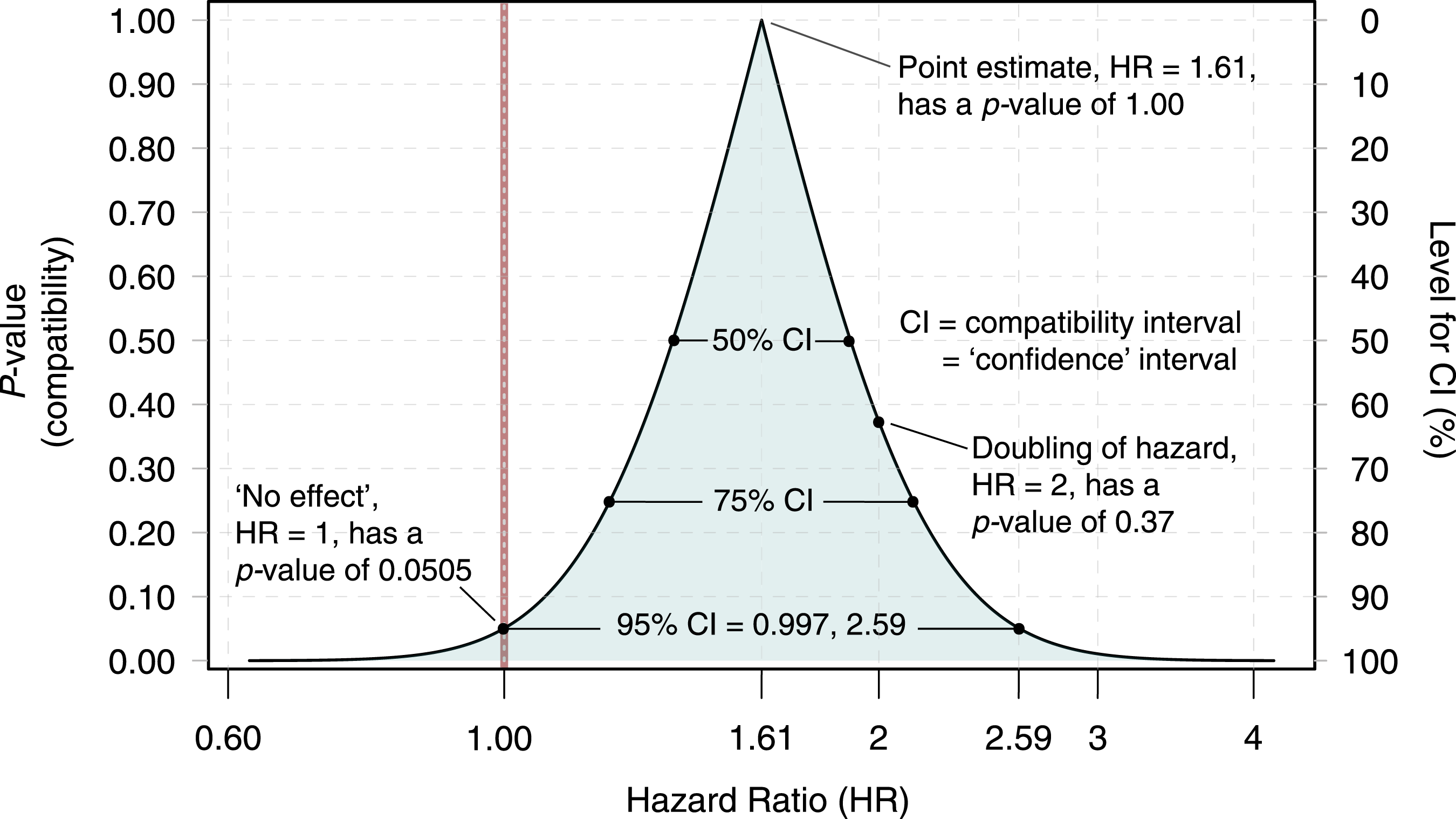

Even if space constraints allow only presentation of intervals, it helps to sketch a compatibility graph in our minds to interpret the interval more correctly (Poole, 1987). We therefore recommend interpreting and referring to confidence intervals as compatibility intervals, showing the effect sizes that have the least information against them (see below) and are thus most compatible with the data and the background model used to compute the interval.

A major advantage of using confidence intervals as compatibility intervals is that it directs our attention to the concrete hypotheses (effect size values) included in the interval, rather than encouraging blurry statements like ‘uncertainty is high’ or ‘low’ (Greenland, 2019b). A focus on the spread of the values contained in the interval helps avoiding falsely declaring ‘no difference’ or ‘no effect’, because the hypothesis of no effect can (and should) be discussed as but one of the many reasonable possibilities inside the interval.

As a further important benefit, describing the interval helps to avoid putting too much emphasis on the point estimate (the observed association). Although the data are most compatible with the effect size given by the point estimate, the interval will usually show that, under the same background model, the data are also reasonably compatible with many other effect sizes.

Another way to see why we should mistrust point estimates is to imagine a compatibility curve as horizontally stacked confidence intervals (Figure 1; Cox, 1958; Birnbaum, 1961; Poole, 1987; Rafi and Greenland, 2020). The peak of the curve showing the observed effect estimate is thus the shortest (0%) confidence interval and is just one point; in other words, point estimates are estimates about which we should have zero confidence (Senn, 2021), even though they have maximum compatibility with the data, given the background model.

Just like a ‘confidence’ interval, a Bayesian posterior-probability (‘credible’) interval can be treated as a compatibility interval, showing effect sizes most compatible with the data under the background model and prior distribution used to compute the interval (Greenland, 2019a). If the data, model, or prior do not inspire ‘confidence’ or ‘credibility’, the interval should not either (McElreath, 2020, Ch: 3). In contrast, ‘compatibility’ does not depend on how correct or incorrect the model assumptions are; it is just a mathematical statement about a relation between the data and the model, however questionable the data or model may be.

S-values to moderate overconfidence

To better appreciate our reasons for switching from ‘significance’ and ‘confidence’ to compatibility, and sense how much or how little evidence a p-value supplies against a hypothesis or model, we advise taking the negative base-2 logarithm of the observed p-value, −log₂(p); this is known as the binary Shannon information, surprisal or s-value (Cole et al., 2021; Greenland, 2019a; Rafi and Greenland, 2020). The s-value is a measure of the information against the model supplied by the test, expressed in units of bits (binary digits), and can be better understood by mapping it to a simple coin-tossing experiment: The s-value is the information against the hypothesis of fairness of the tosses versus loading for heads provided by obtaining s heads in a row (where we round s to the nearest whole number). A 95% compatibility interval is then the range in which the s-value is less than −log₂(0.05) = 4.3. This means that, given the background model, the values in a 95% interval have only about 4 bits or less information against them. These 4 bits equal the information against fairness of coin tosses provided by obtaining four heads in a row, which may be sensed as only modest evidence against fairness and no reason to be confident the coin is either fair or biased for heads (Cole et al., 2021; Greenland, 2019a; Rafi and Greenland, 2020).

Conclusions

We strongly recommend putting the emphasis on explicitly discussing the lower and upper limits of interval estimates showing values that are reasonably compatible with the data, given that all the statistical assumptions in the background model are correct. Even better is to show the p-values for multiple values for the effect size, as in Figure 1 (Infanger and Schmidt-Trucksäss, 2019; Poole, 1987; Rafi and Greenland, 2020; Rothman et al., 2008, Ch: 10). We have provided examples of such descriptions and presentations in Amrhein et al. (2019a, 2019b), Berner and Amrhein (2022), Cole et al. (2021), and Rafi and Greenland (2020). Note however that, just as with p-values and point estimates, the limits of an interval are contingent on the correctness of all background assumptions used to compute the interval; when those assumptions are questionable, the interval may seriously understate the uncertainty warranted about the effect (Greenland, 2005). And even if all assumptions are correct, an interval will bounce around from sample to sample due to random variation (Cumming, 2014; Amrhein et al., 2019a, 2019b). We should therefore not take an observed interval as showing some general truth.

In summary, we agree with Sen et al. (2022) that we should discuss whether the effect estimates represent effect sizes substantial enough to be of practical importance. In doing so, we need to consider much more than the observed point estimate; at the very least we must examine and discuss the effect sizes represented by the limits of our interval estimate. Even better is to visualize how the p-value varies as we move across a table or graph of possible effect sizes.