The effect of machining parameters on surface integrity and fatigue performance of 42CrMo4 + QT high-strength steel

Abstract

This study investigates how machining parameters affect surface integrity and fatigue performance in 42CrMo4 + QT steel. Nine turning setups were tested to evaluate surface roughness, residual stresses, and fatigue strength. Fatigue testing under fully reversed loading (R = –1) at ∼150 Hz revealed that the best fatigue performance occurred in the setup with a cutting speed of 100 m/min, feed rate of 0.1 mm/min, tool nose radius of 0.4 mm, 0.3 mm total finishing depth (over three cuts), and coolant applied. Cutting speed showed the clearest benefit, while other parameters had less predictable effects. Surface roughness did not consistently correlate with fatigue life. Overall, selected machining parameters strongly influence fatigue behavior, though roughness and residual stresses alone do not fully explain the performance trends observed.

Keywords

fatigue strength 42CrMo4 roughness effect residual stress high strength steel

Introduction

High-strength steels are essential in modern engineering, particularly for components subjected to dynamic loading, wear, and high-stress environments. Among these materials, 42CrMo4 + QT (quenched and tempered) steel is notable for its balanced properties, making it suitable for strength-demanding applications. This steel is widely used in sectors such as automotive, aerospace, and heavy machinery, where components like gears, crankshafts, and axles require excellent fatigue resistance alongside toughness and wear resistance.^3,4

Fatigue is a key phenomenon to be studied as it is the biggest factor of failure in loaded structures.^5,6 The fatigue performance of metallic material is highly sensitive to the interplay of material properties, surface conditions, residual stresses, and machining parameters.⁷ Additionally, hard turning processes of 42CrMo4, especially with ceramic or CBN tools and without lubrication, have gained popularity for economic and ecological reasons, though they introduce challenges in controlling surface integrity and roughness.^8–10

Given its critical applications and the complex factors influencing its fatigue performance, 42CrMo4 + QT steel remains a subject of ongoing research and industrial interest. 42CrMo4 is a low-alloy steel¹¹ containing chromium and molybdenum, elements known for their ability to enhance hardenability, high-temperature strength, and corrosion resistance.¹² The steel is normally supplied in the quenched and tempered condition, which involves austenitizing, quenching, and subsequent tempering to refine the microstructure. This process results in a tempered martensitic-bainitic structure that offers a combination of high tensile strength, yield strength, and ductility. These thermal treatments strongly influence mechanical performance, as also demonstrated in heat treatment studies on 42CrMo4 by Chaouch et al.¹³ The material's nominal composition (in wt%) typically includes 0.38–0.45% carbon, 0.90–1.20% chromium, and 0.15–0.30% molybdenum, with minor additions of silicon and manganese. These alloying elements significantly improve its mechanical properties, making it suitable for applications involving cyclic and impact loads. This steel is also used in high wear and load-bearing conditions such as fretting conditions for instance.^14,15 42CrMo4 has low weldability due to its high crack sensitivity^16–18

One of the key parameters influencing high-cycle fatigue is the surface finish of the specimen.¹⁹ In hard turning of 42CrMo4 steel, various machining factors such as feed rate, cutting speed, depth of cut, and tool nose radius directly influence surface roughness and consequently fatigue strength.^8,20

Chen et al.¹⁹ have analyzed the influence of turning speed and feed rate on aluminium alloy 2024 with particular focus on high cycle fatigue. A smoother surface generally enhances fatigue strength by reducing stress concentrations. This effect is demonstrated by Hamad et al.,²¹ who investigated a comparable martensitic-bainitic steel with similar mechanical properties, showing a direct correlation between improved surface quality and increased fatigue strength. Salamanca et al.²² developed a predictive model linking surface roughness and longitudinal residual stress to key machining parameters such as feed rate, depth of cut, and tool nose radius. Their research confirms that surface quality is strongly influenced by the machining setup. It is worth noting that they use the same material from the same batch as it is used in this paper.

Moreover, Özdemir et al.²³ applied the Taguchi method and ANOVA to identify optimal parameters for hard turning of 42CrMo4 steel. Their results showed that surface roughness was most influenced by feed rate, followed by tool tip radius and cutting speed, with the optimal Ra achieved at low feed (0.05 mm/rev), high speed (300 m/min), and shallow cut (0.1 mm).²⁰ Bouacha et al.²⁴ and Suresh et al.²⁵ also showed that RSM could effectively model the influence of machining parameters on surface integrity and cutting forces.

Similarly, Kribes et al.²⁶ used Response Surface Methodology (RSM) to develop predictive models for roughness values in hardened steel turning. Their analysis confirmed that feed rate was the dominant factor, contributing more than 57% to Ra variability and over 61% to Rt variability.^8,27 Though these last mentioned papers focus only on roughness response to the machining parameters, these findings reinforce also the critical role of machining parameters in fatigue-relevant surface characteristics.

The research presented here extends the initial findings^28–30 from the large-scale FABEST project.³¹ While the early phases focused primarily on the size effect,²⁸ subsequent investigations²² revealed the complexity of the issue, uncovering several additional factors influencing the results. Notably, during cyclic loading, dynamic effects led to an unexpected temperature rise,^29,30 producing surface temperatures that are uncommon for steel³² and aluminium alloys.³³ However, similar thermal behaviour has been observed in pure copper materials.³⁴

One of the major challenges in manufacturing metallic parts is turning with good/excellent surface quality, which has a significant effect on the fatigue strength of industrial components. Selecting incorrect or unsuitable values of machining parameters leads to vibration instability in the cutting tool and, as a result, excessive roughness is created on the product's surface.^9,35To achieve this goal, the authors of³⁶ attempted to investigate the simultaneous effects of tool overhang and cutting depth on the static and dynamic deflection of the cutting tool in vitro. After that, the surface roughness was measured in different workpieces. Also, to study the high-cycle fatigue behaviour of products with different surface roughness, four-point bending fatigue test was performed and stress-life diagram (S–N) was obtained. In addition, Basquin coefficients were extracted in terms of surface roughness. Eventually, the mathematical relationship between Basquin coefficients and surface roughness was presented by employing multiple linear regression (MLR) technique. This work was also done to obtain the relationship between machining parameters, including cutting depth and tool overhang, and surface roughness, and finally mathematical relation of life estimation was presented via the studied parameters. Next, S–N diagram of CK45 carbon steel considering surface roughness of 2.07 microns was predicted using the proposed model and different orders (first-, second-, and third-order regression). Comparison of the predicted data with the test results indicated that the mathematical model presented in this research³⁶ is well able to evaluate the fatigue life of carbon steels with different roughness levels.

To reduce this roughness and enhance fatigue life, efforts have been made to optimize cutting conditions. Studies such as those by Ahmed et al.³⁷ and Singh & Rao⁸ show that modeling surface roughness as a function of machining parameters can enable fatigue life prediction based on surface condition. The experimental efficiency of Taguchi's L18 array in machining analysis has also been validated in related studies.^20,38

Three primary effects emerged:

Surface Roughness: Uneven cross-sections of the specimens led to variations in the cutting speed, limited by the capabilities of the available lathe. This, in turn, introduced roughness effects.

Surface Residual Stresses (RS): The combination of sensitive turning conditions and the bulk material's microstructure led to variations in the values and homogeneity of the surface residual stress state.

Specimen Position and Material Hardness: The position of the active part of the specimen within the semi-finished bar influenced the local hardness of the material in the active cross-section, which in turn affected its fatigue response.²⁸

The first two issues were directly related to the machining process used to produce the specimens. These factors likely would not have occurred if the recommended surface preparation procedures outlined in fatigue testing standards^39,40 —such as grinding and longitudinal polishing to remove residual stresses–had been followed. However, it is important to note that these procedures are typically recommendations rather than strict requirements. In this study, the mandatory aspects of the standards were adhered to, but the recommendations were deliberately not applied in order to replicate surface conditions typical of industrial practice. This decision aligned with the objectives of the FABEST project, which emphasized cost-effective manufacturing. The initial target was to achieve an arithmetic mean surface roughness (R_a) of 0.8 μm, but it was in next phases a bit relaxed to reach at maximum 1.2 μm.

It was found, as reported in,²⁸ that specimens with smaller cross-sections could not be produced using turning alone due to low cutting speeds, necessitating subsequent grinding. To maintain cost-effectiveness and closely align with common industrial practices, it was decided to use specimens with an 8 mm active diameter to see the response of specimen properties to various turning conditions. At this diameter, the lathe operating at 4000 rpm could achieve a cutting speed of 100 m/min, which was deemed acceptable for surface quality, as suggested by Zielinski et al.⁴¹

A central issue in the study was the level of residual stresses. The impact of residual stresses during fatigue loading is complex and depends on several factors, particularly the mechanisms of fatigue crack initiation and damage. Residual stresses affect the mean stress value of the cyclic load regime, which is a critical consideration.⁴²

It is important to note that the residual stress state is not merely a macroscopic phenomenon, but a complex superposition of macro, micro, and sub-microscopic stresses. Capek et al.⁴³ highlighted the correlation between macro- and micro-stresses and high-cycle fatigue life. Specifically, tensile macroscopic residual stresses were found to reduce fatigue life. Furthermore, significant changes in microstresses after many cycles were attributed to alterations in dislocation arrangements and grain structures, which are the precursor to fatigue crack initiation.

This study investigated different turning operation setups, with the goal of minimizing or eliminating the need for a subsequent grinding phase. The findings demonstrate how the fatigue life of this steel, commonly used in strength-demanding applications, respond to various machining conditions.

Experimental setup

Material, design of specimens

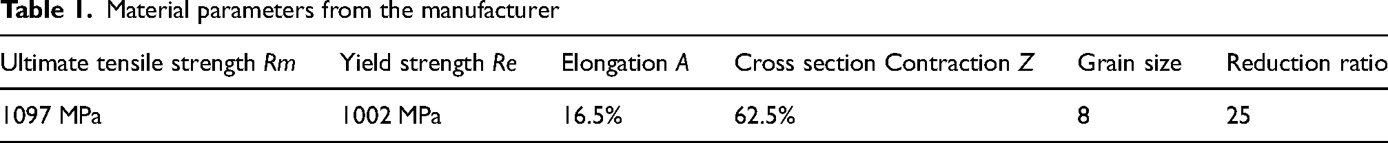
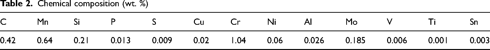
All specimens were produced from a single batch of medium-carbon 42CrMo4 + QT high-strength steel, which was purchased in a quantity of 1.4 tons. The material came in the form of hot-rolled, quenched, and tempered bars, measuring 5–6 meters in length with a nominal diameter of 35 mm. All bars were from the same heat, T46157. The bar manufacturer, TŘINECKÉ ŽELEZÁRNY, a.s., provided the heat data sheet (shown in Table 1), as well as the chemical composition detailed in Table 2. The composition adheres to the ISO 683–17 standard.⁴⁴ The hydrogen content is 1.3 ppm, and nitrogen content is 90 ppm, both of which are well below critical levels. Therefore, hydrogen embrittlement, a phenomenon typically associated with martensitic steels, is not expected to have any adverse impact.

Table 1.

Material parameters from the manufacturer

Ultimate tensile strength Rm	Yield strength Re	Elongation A	Cross section Contraction Z	Grain size	Reduction ratio
1097 MPa	1002 MPa	16.5%	62.5%	8	25

Table 2.

Chemical composition (wt. %)

C	Mn	Si	P	S	Cu	Cr	Ni	Al	Mo	V	Ti	Sn
0.42	0.64	0.21	0.013	0.009	0.02	1.04	0.06	0.026	0.185	0.006	0.001	0.003

The material has limited capacity for plastic deformation, as indicated by the similar yield strength and tensile strength values in Table 1.

The microstructure of 42CrMo4 + QT was analyzed by light optical microscope (LOM) Carl Zeiss Neophot32 equipped with a CCD camera and analytical software Nis Elements AR. For detailed observation, the JEOL JSM-7600F scanning electron microscope (SEM) was used. The metallographic samples were prepared by following steps: wet grinding with SiC paper up to grit P4000, prepolishing with a 3 µm diamond suspension and final polishing with colloidal SiO₂. To reveal the microstructure, the samples were etched with 2% Nital reagent (0.2 ml HNO₃ + 98 ml ethanol). Prior austenitic grains (∼20–25 µm) can be observed together with tempered lath martensite with lowered acicularity, lower fraction of homogeneous bainite, minimum residual austenite and MnS based inclusions (see Figure 1 - left). Detailed analysis (see Figure 1 - right) showed a uniform distribution of fine globular and partially elongated Fe₃C carbides across the martensitic/bainitic blocks and along the martensitic laths. The microstructure of the steel bar is homogeneous along the section.

Figure 1.

Microstructure of 42CrMo4 + QT: (left) LOM micrograph, (right) SEM micrograph

The first attempt to analyze the fatigue response of the sample by the hourglass design was made on the sample A03 (see for example,^28,29 based on the manufacturer's recommendation for the used fatigue testing machine (see Figure 2 - left). To comply with ASTM standards,⁴⁵ the dimensions of all subsequent specimens were slightly modified Figure 2 - right. Both designs feature hourglass design to prevent dangerous undercuts between the fillet and cylindrical central axes, and a thread head with an M16 × 1 thread required to transfer load from the fatigue testing machine.

Figure 2.

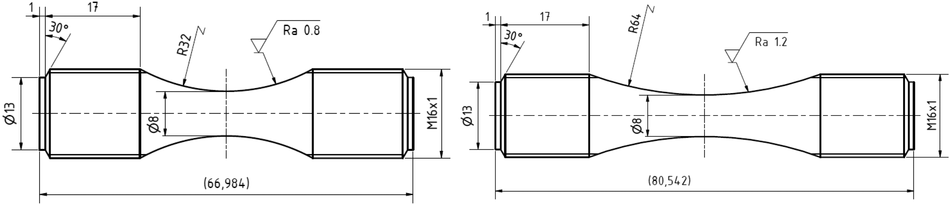
Drawings of the specimen geometries: (left) A03 series; (right) A25 – A37 series. (all measurements indicated in this figure are in millimeters)

Production of specimens (machining parameters)

The specimens discussed in this paper were produced in three distinct phases, all manufactured at VŠB – Technical University of Ostrava:

Phase 0 (Series A03):

This initial phase served as a baseline, where the machining parameters were selected primarily based on standard economic practices. The manufacturer initially assumed that turning alone could achieve the desired surface finish (Ra = 0.8 µm). However, the resulting surface quality fell short of expectations, requiring manual grinding to meet the roughness target and making A03 the only series not finished by turning alone. This deviation was avoided in all subsequent phases to preserve the influence of turning parameters on fatigue behaviour. Phase 0 highlighted the sensitivity of fatigue performance to surface condition and confirmed the need for a more controlled and systematic parameter selection in subsequent phases.

Phase 1 (Series A25–A29):

Informed by the limitations observed in Phase 0, this phase explored a range of machining conditions by varying key parameters such as cutting speed, feed rate, and finishing cut depth. The goal was to understand their individual and combined effects on surface roughness, residual stresses, and ultimately fatigue performance. Grinding was not permitted, allowing the isolated influence of turning to be studied. The finishing depth in this phase was fixed at 0.3 mm (cumulative of the last three cuts). From this moment on, the target roughness in the production was more relaxed to achieve at maximum Ra = 1.2 μm.

Phase 2 (Series A35–A37):

Based on both the experimental results from Phase 1 and published literature e.g.,^22,41 the third phase introduced targeted refinements to enhance surface integrity. The feed rate was reduced to 0.05 mm/rev and the cutting speed was maximized at 100 m/min–two changes known to improve surface finish and reduce tensile residual stresses. In addition, the total finishing cut depth was increased to 0.5 mm, aimed at removing deeper material layers potentially affected by roughing-induced stresses. These changes were implemented with the intention of improving fatigue performance through optimized surface preparation.

All specimens were manufactured on a DMG Mori NLX 2500MC/700 machine. In every case, rough cuts were made using the Decocut 1040 process fluid, with a cutting depth of 0.5 mm. The tooling included the C4-PDJNR-27055-15HP insert holder and Sandvik Coromant inserts: DNMG 15 06 08-MM 1125 (with a nose radius of 0.8 mm) and DNMG 15 06 04-SM 1125 (with a nose radius of 0.4 mm). The specific machining setups for each phase are outlined in Table 3. Notably, in Phase 1, the cutting speed varied between 62.8 m/min and 100.5 m/min at the smallest diameter of the specimens (the critical zone for fatigue), along with variations in feed rate and final cut depth. For all specimens in Phase 1, the last three cuts were combined to a total cut height of 0.3 mm. It needs to be mentioned that the spindle speed is kept constant and the indicated cutting speed in Table 3 is reached at the D = 8 mm, elsewhere the cutting speed is higher.

Table 3.

Different turning parameters used for machining the fatigue samples for series A03, A25-A29 and A35-A37. All series were turned without additional grinding or polishing except A03 where manual grinding was performed

Parameter		Series
Parameter		A03	A25	A26	A27	A28	A29	A35	A36	A37
Cutting speed at D = 8 mm	v_c [m/min]	100.5	75	75.4	100	62.8	75.4	100	100	100
Spindle speed	[1/min]	4000	2984	3000	3979	2500	3000	3979	3979	3979
Feed rate	F [mm/min]	0.1	0.05	0.05	0.1	0.1	0.1	0.05	0.05	0.05
Cooling fluid (last cuts)		x	x		x			x	x	x
Cutter nose radius	R [mm]	0.4	0.4	0.4	0.4	0.4	0.4	0.8	0.4	0.4
Last cut height	h₁ [mm]	0.1	0.05	0.1	0.1	0.05	0.1	0.1	0.05	0.1
Second-last cut height	h₂ [mm]	0.5	0.1	0.1	0.1	0.1	0.1	0.2	0.15	0.2
Third-last cut height	h₃ [mm]	0.5	0.15	0.1	0.1	0.15	0.1	0.2	0.3	0.2

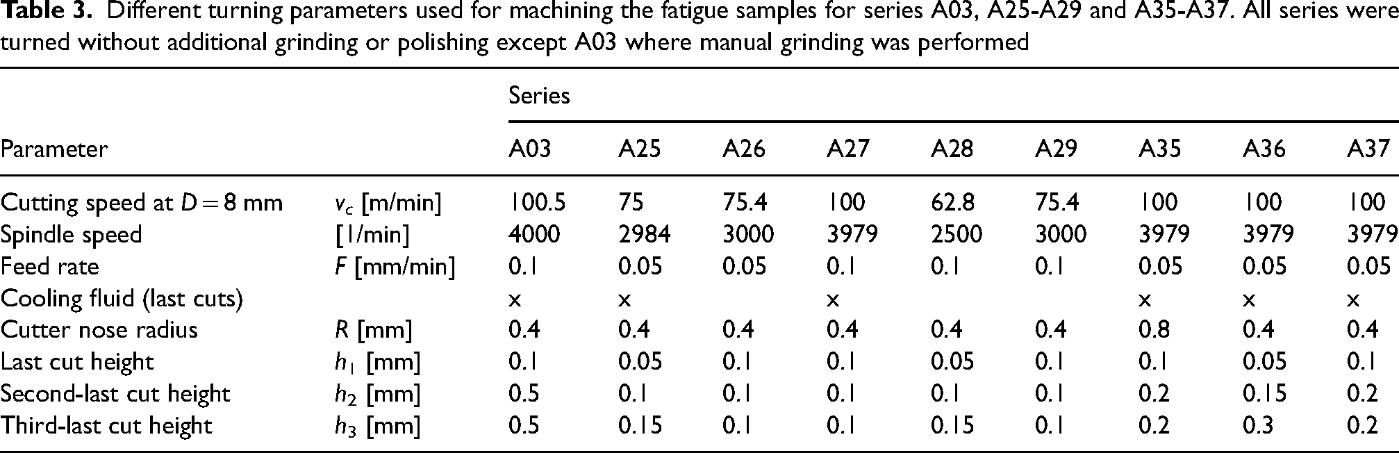
Based on the findings of Zielinski et al.⁴¹ and the fatigue performance observed in Phase 1, the cutting speed for Phase 2 was set to the maximum value of 100 m/min. It is worth mentioning that this is practically typical maximum cutting speed for a specimen of the minimum diameter of 8 mm, because many lathes cannot exceed 4000 rpm. If other authors refer to higher cutting speeds, they likely focused on manufacturing specimens of significantly bigger diameters. The key differences in Phase 2 were the cutter nose radius (set to 0.8 mm for A35) and the configuration of the final three cut heights. These adjustments were designed to achieve a combined total height of 0.5 mm for the last three cuts. This approach aimed to remove a deeper layer of material, which was presumed to be significantly influenced by residual stresses introduced during the earlier roughing phase. Moreover, the machining parameters selected for Phase 2—specifically the reduced feed rate of 0.05 mm/rev and the high cutting speed–were based on both the outcomes of Phase 1 and previous literature e.g.,^22,41 which indicate that lower feed rates and higher cutting speeds generally improve surface finish and reduce tensile residual stresses. These refinements were therefore not arbitrary but reflect a deliberate strategy to enhance fatigue performance through improved surface conditions.

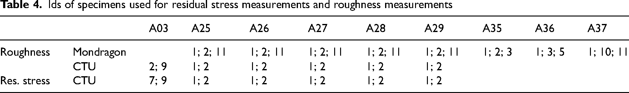
As regards the specimens from each series chosen for the subsequently described measurements, the list of their IDs is provided in Table 4.

Table 4.

Ids of specimens used for residual stress measurements and roughness measurements

		A03	A25	A26	A27	A28	A29	A35	A36	A37
Roughness	Mondragon		1; 2; 11	1; 2; 11	1; 2; 11	1; 2; 11	1; 2; 11	1; 2; 3	1; 3; 5	1; 10; 11
Roughness	CTU	2; 9	1; 2	1; 2	1; 2	1; 2	1; 2
Res. stress	CTU	7; 9	1; 2	1; 2	1; 2	1; 2	1; 2

State of residual stress

Macroscopic residual stress measurements were performed on each series, with the number of measurements per series specified in Table 4. For each configuration, residual stresses were measured on at least two specimens, and in most cases, three specimens were analyzed to ensure reproducibility. The measurements were conducted using X-ray diffraction at the Czech Technical University in Prague. During the analysis, the specimen was slowly rotated, and the reported values represent an average taken along the full circumference at the measurement location.

To ensure consistency, residual stresses were measured at the location of the smallest diameter–referred to as the hot spot–where stress amplitudes during fatigue testing are highest and cracks are most likely to initiate. This location corresponds to the same region where surface roughness measurements were performed, facilitating direct correlation between surface integrity and fatigue performance.

For the A03 experiments, residual stress measurements were conducted only after constant-amplitude, load-controlled fatigue tests, where lifetimes exceeded 1 million cycles in both cases. Despite the extended number of cycles, the measurements intentionally avoided the hot-spot region (where cracking occurred), as this area could experience a significant alteration due to cyclic loading. Instead, measurements for A03 were taken 8 mm away from the minimum diameter, a location with substantially lower local stresses during loading. In all other cases, measurements were conducted at the minimum diameter, where the critical stress is reached.

Lattice deformations of the diffraction lines Kα1 of the planes {211} of the ferrite phase were analyzed using the X´Pert Pro MPD diffractometer with chromium radiation. The diffraction angles 2θ^hkl were determined by using the Pearson VII function and the Rachinger method. Standard X-ray elastic constants ½s₂ = 5.76 TPa^–1, s₁ = –1.25 TPa^–1, and the sin²ψ method were used to calculate the state of residual stress. The irradiated volume was defined by the geometry of the experiment, the rotation of the specimens, the effective penetration depth of the X-ray radiation (approx. 5 µm), and the pinhole size (0.25 × 0.3 mm²).

Roughness measurements

Surface roughness measurements were performed independently at CTU in Prague and Mondragon University, using different equipment and methodologies:

M1 measurement type: At CTU, a Mahr MarSurf LD 120 mechanical profilometer was used to measure roughness along a single longitudinal path located at the smallest-diameter section of the specimen–the fatigue-critical hot-spot. The total measurement length was defined based on five Rsm wavelengths to provide high-resolution data from this region. At CTU, the reported roughness is based on a single measured length of five wavelengths taken from the central section of the specimen.

M2 measurement type: Phase 0 and Phase 1 series (A03-A29) were measured at Mondragon University using a Mitutoyo Surftest SJ-210 device with the measurement length analyzed at six positions: three at the central hot-spot region, spaced 90° apart around the circumference, and three closer to the specimen heads. The addition of measurements out of the center zone responded to a specific issue observed in the central zone of the specimens: a step-like surface defect resulting from machining. These out-of-center points were selected within the region subjected to steady-state cutting and do not correspond to areas with significant variations in cutting speed, as they remain relatively close to the central zone in terms of geometry and cutting conditions.

M3 measurement type: To increase consistency of measurements at Mondragon University and their comparability with the CTU method, only the measurements in the central minimum cross-section were kept. The original trio of measurements at angle 0, 90 and 180 degrees was replenished by measurements at three more angular positions at 45, 240 and 300 degrees.

Fatigue tests

Fatigue tests were conducted using the Amsler HFP422 resonator, which operates near the resonance frequency of the machine-specimen system. For the specific specimen design used consistently throughout the testing campaign, the load frequency remained. In this setup, the operating frequency was approximately in the range of 152–154 Hz.

All tests were performed under fully reversed push-pull loading. Each test was concluded either by the obvious rupture of the specimen or upon exceeding one of the pre-established criteria:

Frequency drops by 5 Hz (Phase 0), 22 Hz (Phase 1 and 2).

The load amplitude changes by ±0.2 kN (Phase 0), ± 0.5 kN (Phase 1 and 2).

Mean load changes by ±0.5 kN (all series).

2·10⁷ cycles are reached. These specimens are classified as run-outs.

Main focus in this paper was focused on the area of High Cycle Fatigue (HCF) with transition to the fatigue limit (σ_FL) domain.

In Phase 0, fatigue tests were stopped when a frequency drop of 5 Hz was detected, while in Phases 1 and 2, the threshold was adjusted to 22 Hz to better reflect the higher operating frequency (∼150 Hz) and ensure consistent detection of crack propagation onset. This change does not affect the comparability of S–N data, as the frequency drop occurs very rapidly near failure, and differences in cycle count at this stage are negligible in the high-cycle fatigue regime.

Results

Roughness values

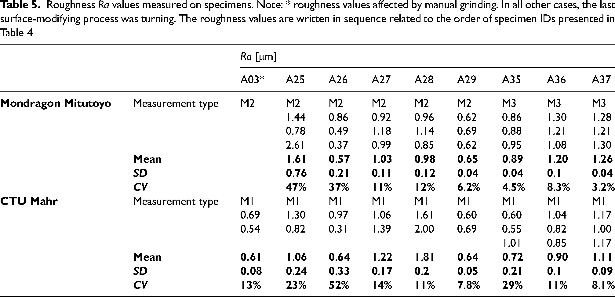
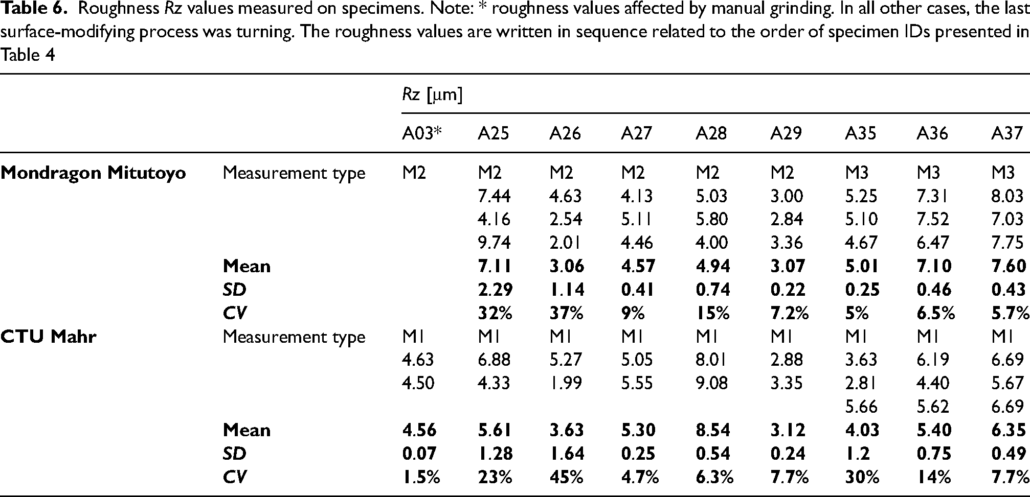
The roughness values achieved are shown in Table 5 and Figure 3 for the Ra parameter and in Table 6 for the Rz parameter. The reported values are shown for two or three specimens per series, and measurements by both mentioned machines.

Figure 3.

Bar plot of roughness Ra and Rz (mean value with indicated standard deviation) values measured on specimens comparing measurements at Mondragon and CTU in Prague without A03 (mean Ra = 0.61 and Rz = 4.56) which has not been measured at both facilities

Table 5.

Roughness Ra values measured on specimens. Note: * roughness values affected by manual grinding. In all other cases, the last surface-modifying process was turning. The roughness values are written in sequence related to the order of specimen IDs presented in Table 4

		Ra [μm]
		A03*	A25	A26	A27	A28	A29	A35	A36	A37
Mondragon Mitutoyo	Measurement type	M2	M2	M2	M2	M2	M2	M3	M3	M3
			1.44	0.86	0.92	0.96	0.62	0.86	1.30	1.28
			0.78	0.49	1.18	1.14	0.69	0.88	1.21	1.21
			2.61	0.37	0.99	0.85	0.62	0.95	1.08	1.30
	Mean		1.61	0.57	1.03	0.98	0.65	0.89	1.20	1.26
	SD		0.76	0.21	0.11	0.12	0.04	0.04	0.1	0.04
	CV		47%	37%	11%	12%	6.2%	4.5%	8.3%	3.2%
CTU Mahr	Measurement type	M1	M1	M1	M1	M1	M1	M1	M1	M1
		0.69	1.30	0.97	1.06	1.61	0.60	0.60	1.04	1.17
		0.54	0.82	0.31	1.39	2.00	0.69	0.55	0.82	1.00
								1.01	0.85	1.17
	Mean	0.61	1.06	0.64	1.22	1.81	0.64	0.72	0.90	1.11
	SD	0.08	0.24	0.33	0.17	0.2	0.05	0.21	0.1	0.09
	CV	13%	23%	52%	14%	11%	7.8%	29%	11%	8.1%

Table 6.

Roughness Rz values measured on specimens. Note: * roughness values affected by manual grinding. In all other cases, the last surface-modifying process was turning. The roughness values are written in sequence related to the order of specimen IDs presented in Table 4

		Rz [μm]
		A03*	A25	A26	A27	A28	A29	A35	A36	A37
Mondragon Mitutoyo	Measurement type	M2	M2	M2	M2	M2	M2	M3	M3	M3
			7.44	4.63	4.13	5.03	3.00	5.25	7.31	8.03
			4.16	2.54	5.11	5.80	2.84	5.10	7.52	7.03
			9.74	2.01	4.46	4.00	3.36	4.67	6.47	7.75
	Mean		7.11	3.06	4.57	4.94	3.07	5.01	7.10	7.60
	SD		2.29	1.14	0.41	0.74	0.22	0.25	0.46	0.43
	CV		32%	37%	9%	15%	7.2%	5%	6.5%	5.7%
CTU Mahr	Measurement type	M1	M1	M1	M1	M1	M1	M1	M1	M1
		4.63	6.88	5.27	5.05	8.01	2.88	3.63	6.19	6.69
		4.50	4.33	1.99	5.55	9.08	3.35	2.81	4.40	5.67
								5.66	5.62	6.69
	Mean	4.56	5.61	3.63	5.30	8.54	3.12	4.03	5.40	6.35
	SD	0.07	1.28	1.64	0.25	0.54	0.24	1.2	0.75	0.49
	CV	1.5%	23%	45%	4.7%	6.3%	7.7%	30%	14%	7.7%

The A03 series is not evaluated in Figure 3 regarding the effect of the turning setup on the final surface roughness quality, as its production involved a final manual grinding phase. The roughness measurements for the A25 and A26 setups exhibit significant scatter in both Ra and Rz values, indicating a lack of consistency in the manufacturing process. Despite this variability, the A26 setup achieved some of the lowest roughness values observed within the scope of the tests, highlighting its potential for improved surface quality under optimized conditions.

The difference in roughness values measured at Mondragon and CTU for the A28 specimens is notable: the magnitude of the values differs significantly, although the relative difference between specimens 1 and 2 remains similar. This discrepancy may stem from differences in signal processing methodologies. For A28 specimens, additional measurements conducted at CTU out of the central position revealed significantly lower roughness values compared to the measurements in the center. When such values are included in the averaging process, they can lead to lower overall roughness values, as observed in Mondragon's results. For other Phase 1 specimens, such pronounced differences based on the longitudinal position of the measured length were not observed.

Among all configurations, scenarios A26 and A29 exhibit the most favorable surface roughness values, depending on the measurement source. While A29 shows the lowest and most consistent roughness values in the CTU dataset, A26 achieves the lowest average Ra values across both CTU and Mondragon measurements, aligning more closely with the target Ra of 0.8 μm. This outcome is consistent with expectations, as A26 was machined with a lower feed rate (0.05 mm/rev vs. 0.1 mm/rev in A29), a parameter known to reduce both surface roughness and tensile residual stresses. In contrast, the Phase 2 setups (A35–A37) meet only the more relaxed roughness target related to modified specimen type with higher requested allowable roughness Ra = 1.2 μm, with only A35 approaching acceptable levels.

Residual stresses

The residual stress values summarized in Table 7 and Figure 4 are derived from post-processing individual measurements, capturing the minimum and maximum residual stresses in each direction across multiple specimens (n in Table 7) of each evaluated series. Specifically, the first value in the X ± Y format represents the mean of the minimum and maximum stresses obtained from all measured specimens. This is not an average stress value itself but rather a midpoint of the extreme values. The Y-value denotes half of the range (span) between the minimum and maximum residual stresses for the given configuration.

Figure 4.

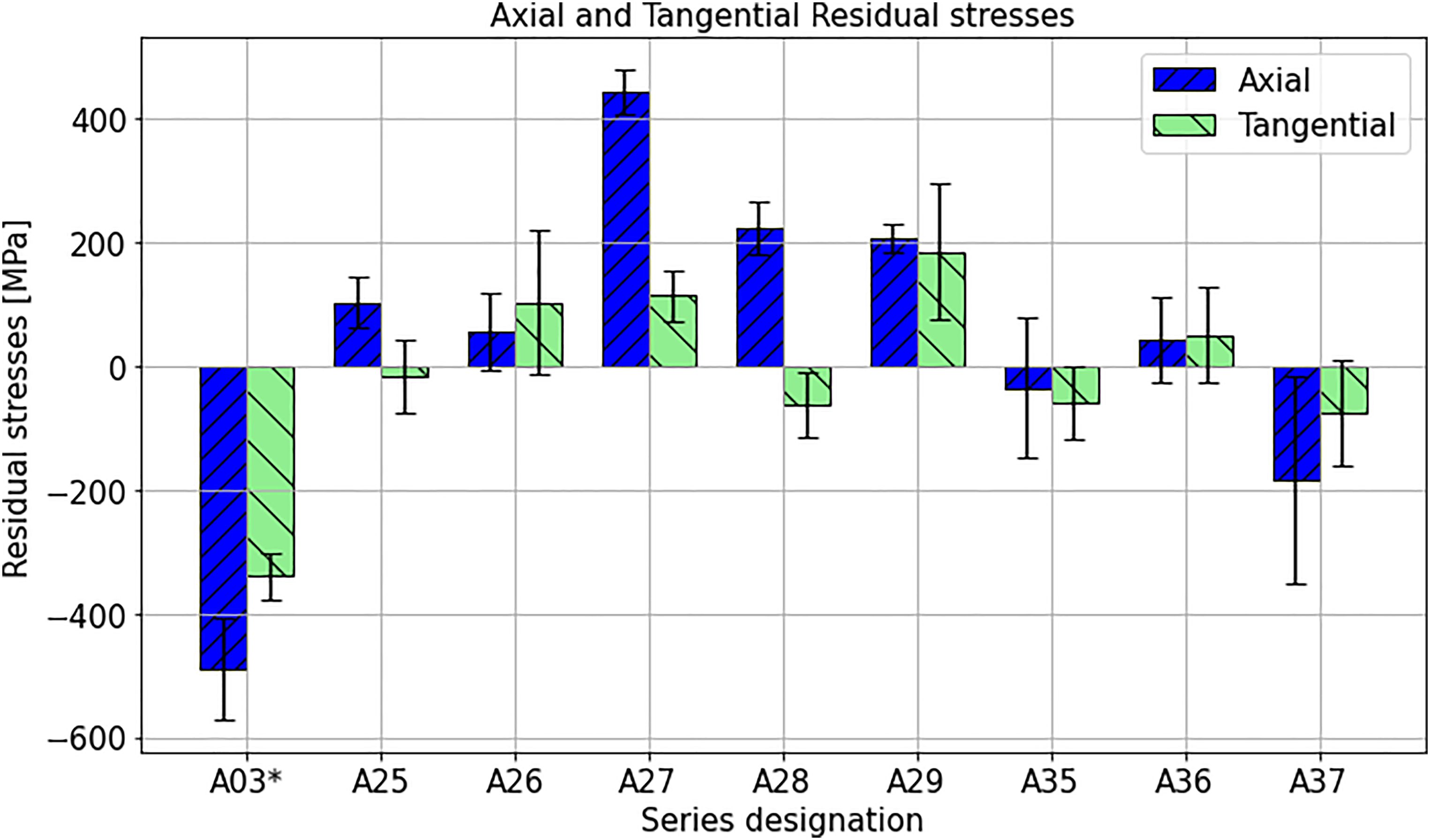
Bar plot of statistically processed results of macroscopic residual stresses. Note: * In the case of A03 experiments, the values were obtained after the fatigue tests were finalized. They relate to the location 8 mm away from the minimum diameter, which should be minimally affected by the preceding loading

Table 7.

Statistically processed results of macroscopic residual stresses, explained in the text. Note: * In the case of A03 experiments, the values were obtained after the fatigue tests were finalized. They relate to the location 8 mm away from the minimum diameter, which should be minimally affected by the preceding loading

Series	Residual stresses in MPa
Series	Axial	Tangential
A03*	−490 ± 81	−340 ± 39
A25	102 ± 42	−17 ± 60
A26	55 ± 61	102 ± 116
A27	442 ± 35	113 ± 40
A28	222 ± 42	−62 ± 53
A29	207 ± 23	184 ± 109
A35	−36 ± 114	−60 ± 59
A36	43 ± 69	49 ± 77
A37	−184 ± 168	−76 ± 85

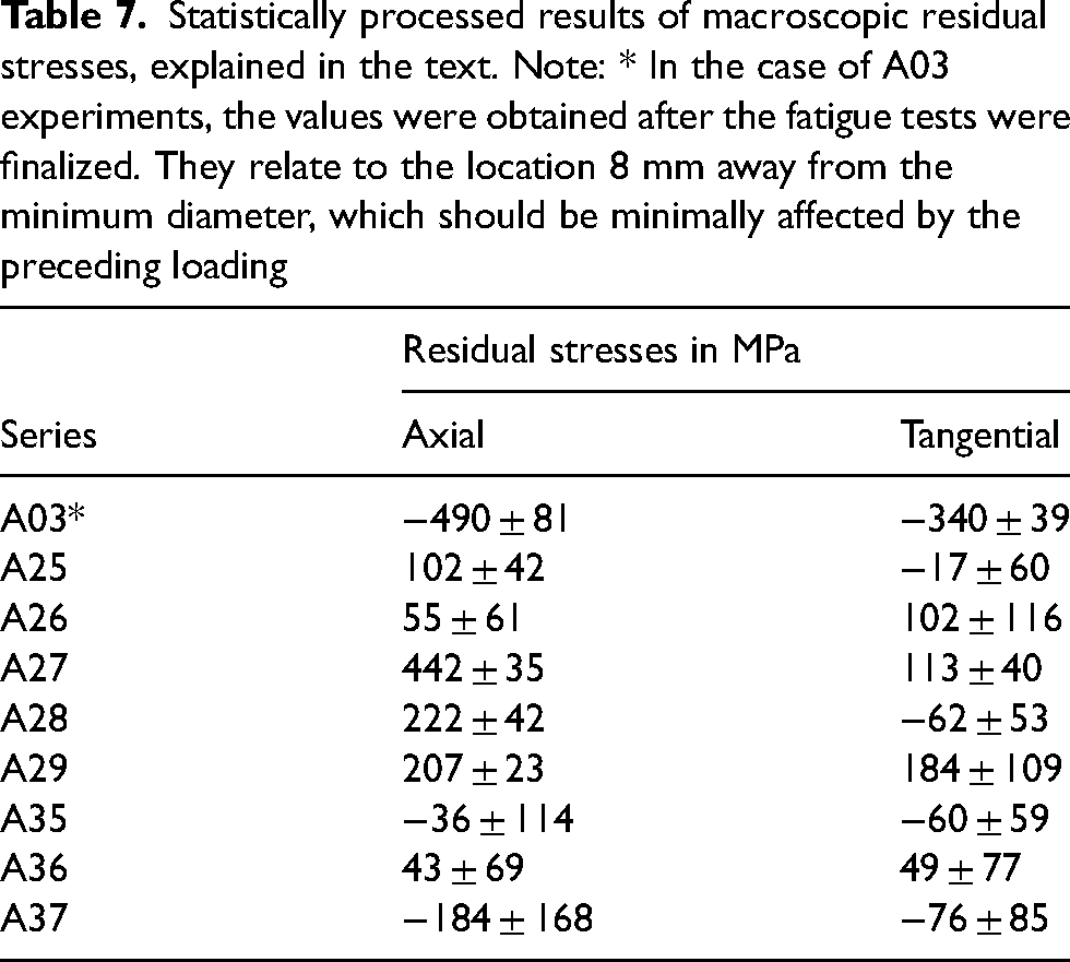
The results in Table 7 and Figure 4 represent overall residual stress levels. A wide variation in residual stress values across all series is observed, ranging from −490 MPa (compression, A03 setup) to 442 MPa (tension, A27 setup) in the axial direction. Among these configurations, A26, A35, and A36 exhibit residual stress values closest to zero. A clear directional dependency is evident, with higher tensile stresses typically present in the axial direction and lower stresses in the tangential direction. The exception is the A29 setup, which displays a nearly equibiaxial stress state despite pronounced stress magnitudes.

In terms of axial residual stresses, the A03 configuration stands out as particularly favorable due to its high compressive stress levels. However, while moderate compressive stresses are known to delay crack initiation and enhance fatigue life, excessively high compressive stresses can become counterproductive by promoting local plasticity, stress relaxation, or early crack growth. Similarly, the A37 series exhibits significant compressive axial stresses, but the variability is large, with measured values ranging from approximately zero to −350 MPa. This series demonstrates the largest scatter of residual stresses among all configurations, indicating inconsistent quality of the manufactured product. The A35 configuration also shows considerable scatter, though centered around nearly zero residual stress values, further reflecting variability in process stability.

Surface artefact

Interestingly, a consistent and repeatable groove was observed in the middle of the specimen's surface, regardless of the machining parameters (see Figure 5). This groove deviates from the regular surface profile by approximately 10 μm, measured between the highest peak and the lowest point, and extends over a length of 400–500 μm. Given that the machining conditions were deliberately varied across the series without affecting the occurrence of the groove, errors in the turning parameters can be ruled out.

Figure 5.

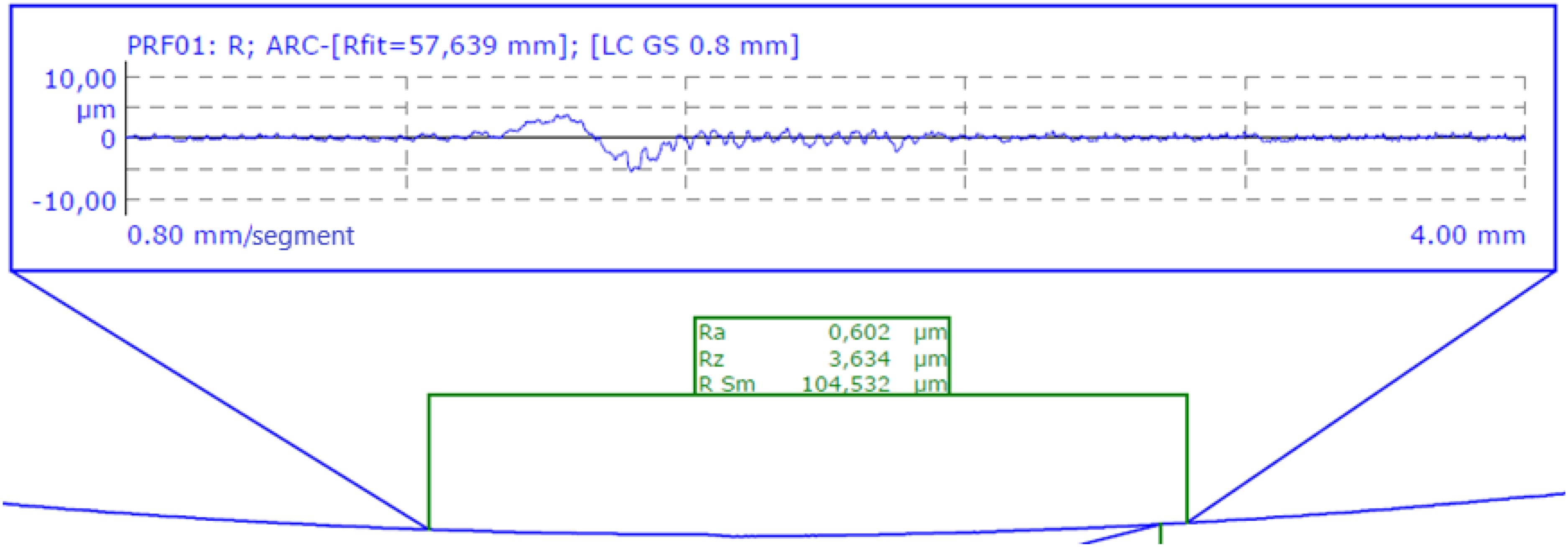
Roughness profile of the A35 specimen, revealing a small groove with a ∼10 μm deviation located at the midpoint of the specimen. This region corresponds to the area of the smallest diameter, which is subjected to the highest stress amplitude during fatigue testing

The most plausible explanation lies in the machining process itself. As the cutting tool transitions between the two specimen heads while shaping the radius, it undergoes a trajectory change–from moving inward to the specimen axis to shifting outward. It is likely that a slight clearance in the lathe mechanism contributes to this irregularity, introducing a subtle deviation at a specific point in the process.

The groove is uniformly present in all roughness measurement paths analyzed in M1 measurement type. Because it is a single artefact in the longitudinal direction, its peak value affects rather the Rz value which focuses on maximum and minimum height of the profile than it affects Ra value, in which its effect diminished. Based on the roughness of the surface nearby, the importance of this single artefact is highlighted or diminished for individual series.

When the implications of this artefact were analyzed after the tests, a question was placed if it does not affect also the residual stress distribution. If the theory of the machine clearance was true, the loads induced by the tool should diminish at some longitudinal position along the tool path. It was decided to analyze this effect by several residual stress measurements along the specimen longitudinal axis. For this experiment however, another material and semi-product was used, because the specimens described in this paper have already been broken. The analyzed specimen of the type used for Phases 1 and 2 was fabricated from the high-strength steel 36NiCrMo6 +QT.

The axial residual stress profiles in Figure 6 refer to several locations in the longitudinal direction and show that the impact of the turning artefact on residual stress distribution can be significant. It must be admitted that the steep stress gradient around the central location obscure the exact value of residual stress, if only one value along the specimen length was obtained in all previous cases. The peak decrease in residual stress value can be in tens of percents from the nominal value. It can be only guessed to which extent such change projects into the final fatigue life. It is obvious that more care must be dedicated into exact localization of the residual stress measurements in further experiments.

Figure 6.

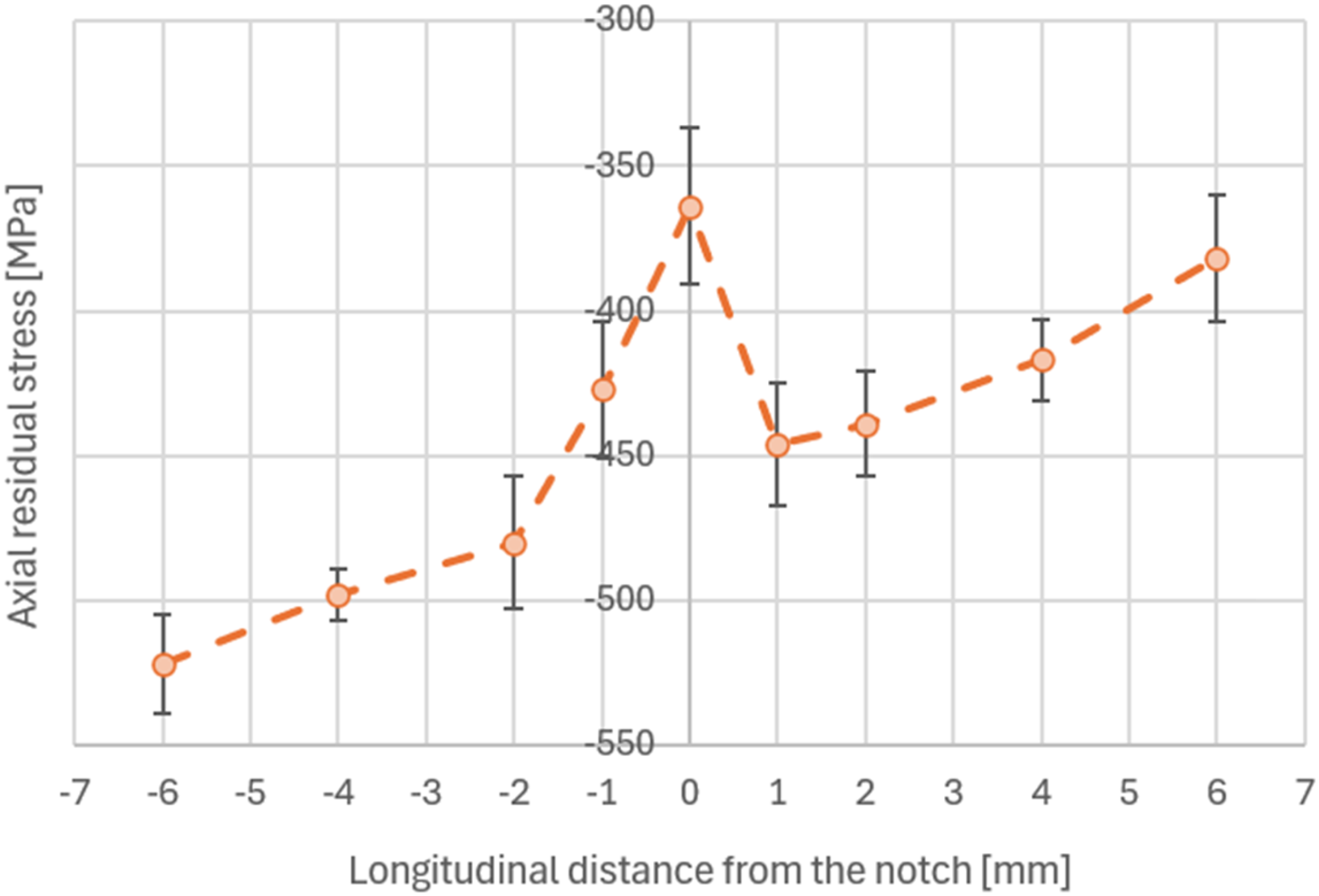
Axial residual stress values measured along the specimen longitudinal axis

Fatigue strengths

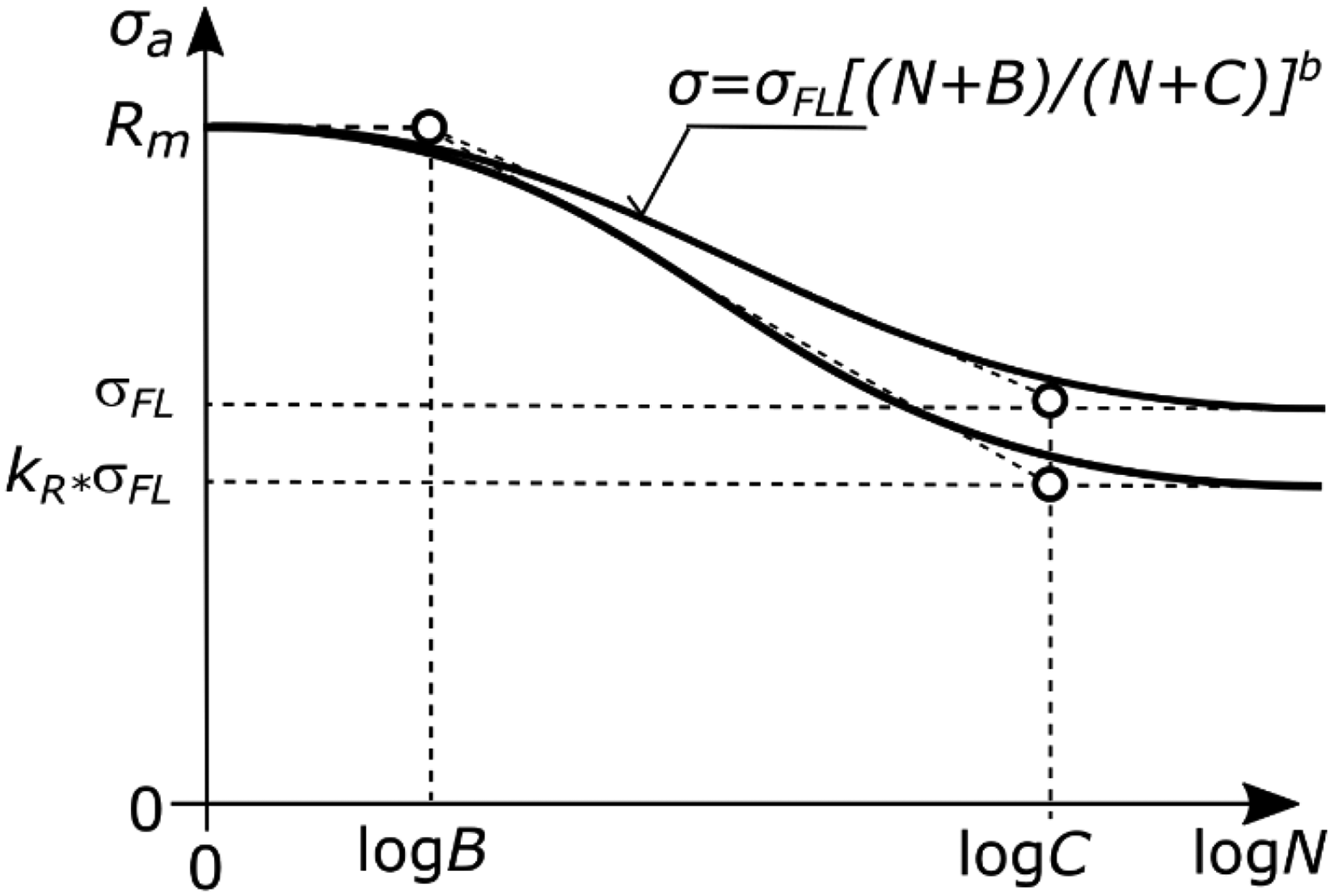
The fatigue response is illustrated in the two graphs presented in Figure 7 and Figure 8. The series corresponding to the machining setups Axx are represented as fatigue curves FABxx (as that indicates the connection to the FABER project). In addition to the data points for each configuration, the fatigue curves were derived using regression based on the Kohout-Věchet equation^46,47: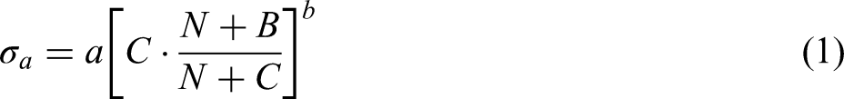

σ_{a} = a {[C \cdot \frac{N + B}{N + C}]}^{b}

(1)

Figure 7.

S-N curves of specimens from series A03 to A29. Ra refers to the roughness parameter and RS refers to residual stresses where a and t concern axial and tangential directions, respectively

Figure 8.

S-N curves of specimens from the best performing series from Phases 0, 1 and Phase 2. Ra refers to the roughness parameter and RS refers to residual stresses where a and t concern axial and tangential directions, respectively

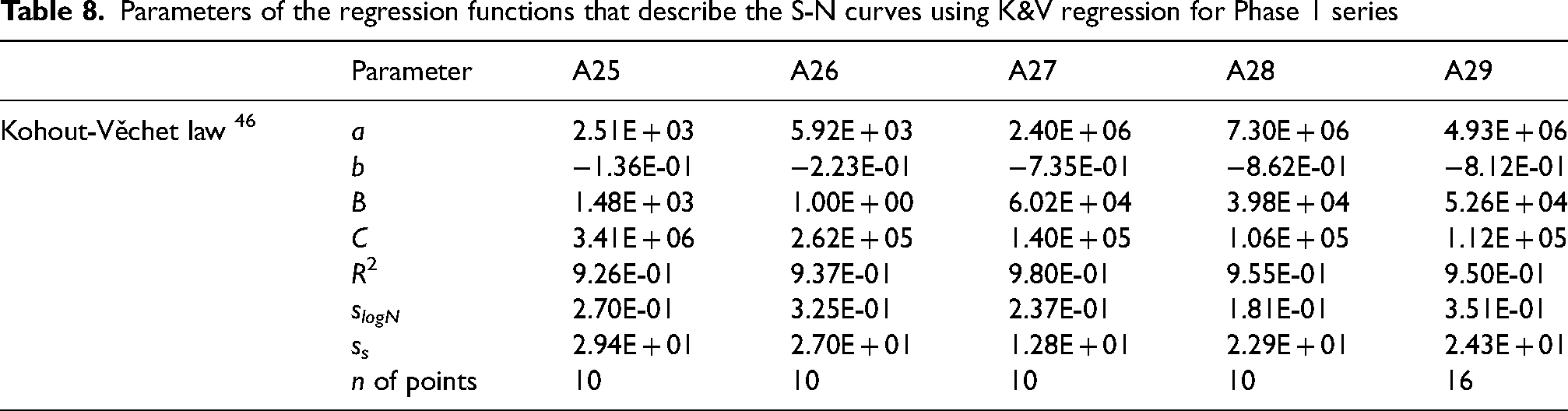
In this model, σ_a is the applied stress amplitude and N is the number of cycles to failure. The parameters a and b are material constants, where a represents a fatigue strength coefficient (scaling factor – for large N, the fatigue strength asymptotically approaches the fatigue limit at a·C^b) and b defines the slope of the S–N curve on a log-log scale. The constants B and C are nbers of cycles at the transition between quasi-static region and the inclined part and the inclined part and the fatigue limit region, respectively, ensuring a smooth and continuous curve across the full range of fatigue lives. This formula is effective in capturing fatigue behaviour as it transitions from the typical power-law region in the finite-life domain to the region approaching the conventional fatigue limit. Parameters of K&V regressions are in Table 8 (Phase 1) and Table 9 (Phases 0 and 2).

Table 8.

Parameters of the regression functions that describe the S-N curves using K&V regression for Phase 1 series

	Parameter	A25	A26	A27	A28	A29
Kohout-Věchet law ⁴⁶	a	2.51E + 03	5.92E + 03	2.40E + 06	7.30E + 06	4.93E + 06
	b	−1.36E-01	−2.23E-01	−7.35E-01	−8.62E-01	−8.12E-01
	B	1.48E + 03	1.00E + 00	6.02E + 04	3.98E + 04	5.26E + 04
	C	3.41E + 06	2.62E + 05	1.40E + 05	1.06E + 05	1.12E + 05
	R ²	9.26E-01	9.37E-01	9.80E-01	9.55E-01	9.50E-01
	s_logN	2.70E-01	3.25E-01	2.37E-01	1.81E-01	3.51E-01
	s_s	2.94E + 01	2.70E + 01	1.28E + 01	2.29E + 01	2.43E + 01
	n of points	10	10	10	10	16

Table 9.

Parameters of the regression functions that describe the S-N curves using K&V regression for Phase 0 and Phase 2 series

	Parameter	A03	A35	A36	A37
Kohout-Věchet law ⁴⁶	a	2.22E + 04	1.39E + 03	2.00E + 06	2.89E + 08
	b	−3.14E-01	−7.21E-02	−6.79E-01	−1.09E + 00
	B	7.30E + 04	5.96E + 04	1.36E + 05	1.46E + 05
	C	2.00E + 05	1.04E + 14	2.43E + 05	2.48E + 05
	R ²	9.84E-01	9.73E-01	8.60E-01	9.53E-01
	s_logN	2.44E-01	2.20E-01	6.24E-01	2.20E-01
	s_s	9.88E + 00	1.68E + 01	3.26E + 01	2.03E + 01
	n of points	10	5	7	8

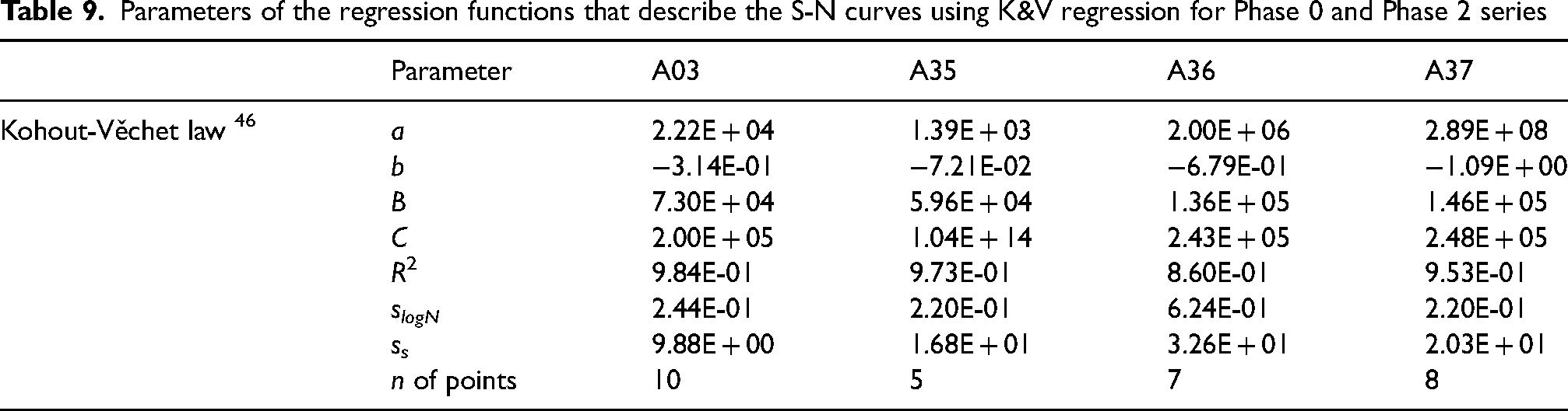
Figure 7 refers to the results from Phase 0 (A03 series, which were manually ground to achieve the desired roughness) and Phase 1 (series A25–A29). Without the available residual stress measurements (see Table 7 and Figure 4), which reveal the extreme compressive residual stresses of the A03 configuration, the superior performance of the A03 series would be challenging to interpret as the A03 series demonstrates the best fatigue performance among these series.

When evaluating the performance of specimens in Phase 1, the fatigue curves associated with A27, A29, and A25 exhibit superior performance compared to A26 and A28. The poorest results are observed for the A28 setup, likely due to its use of the lowest cutting speed across all combinations. The second lowest fatigue performance is seen with the A26 setup. Although A26 and A28 share the same cut area (0.05 mm x 0.1 mm) with transposed sides, A26 employs a higher cutting speed. This may account for its lower roughness values and reduced residual stresses, resulting in an improved fatigue response compared to A28. It can be hypothesized that achieving an optimal cutting speed is crucial for proper chip formation while minimizing unnecessary plastic deformation and the associated residual stresses, thereby enhancing fatigue performance.

The slightly poorer performance of A25 beyond 1 million cycles is primarily influenced by a single outlier data point. This outlier notably affects the position of the fatigue curve near its vicinity, as it lies close to the boundary of the interpolated region. The A25 fatigue curve also displays a significantly higher scatter of data points compared to the other curves, with the exception of A26. This increased scatter is likely linked to the variability in roughness values observed for A25, as detailed in Table 5 and Table 6 with visualization of Ra roughness.

Considering the high residual tensile stresses induced by the A27 setup, it is surprising that it achieves the best fatigue performance among the Phase 1 experiments. The A29 setup follows closely behind, despite its superior roughness values and lower residual stresses compared to A27. The position of the A29 fatigue curve is notably influenced by the greater scatter of its data points, which exhibit twice the standard deviation in stresses compared to the A27 curve. Although the residual stress and roughness measurements for the A29 setup indicate high homogeneity, this curve is based on 16 data points, in contrast to the 10 data points used for the other series. This might mean the specimens analyzed for roughness and residual stresses may not fully represent the variability in the A29 setup.

An intriguing observation from the experiments in Phases 0 and 1, as illustrated in Figure 7, is that above a stress amplitude of 600 MPa, the influence of residual stresses appears to diminish to the point where the fatigue curves converge. This occurs despite the yield strength of this batch of QT steel being 1003 MPa. In this high-stress region, the regression curves are typically influenced by only one or two data points, making it difficult to assess any residual surface stress and roughness effects based on these observations.

The results of Phase 1 suggested that surface roughness values and residual stress measurements taken directly on the surface may not fully explain the observed fatigue performance. A key undocumented factor could be the residual stress profile beneath the surface. It was hypothesized that overly shallow final cuts might have partially removed the residual stress profile near the surface, inadvertently exposing regions of high tensile stresses that would otherwise remain deeper within the material. To address this, Phase 2 designs were modified to remove 0.5 mm of material with the last three finishing cuts, compared to the 0.3 mm removed in Phase 1 specimens. Additionally, based on research by Zielinski et al.,⁴¹ a cutting speed of 100 m/min was chosen, corresponding to a spindle speed of 4000 rpm for the smallest specimen diameter.

The adjustments made to the turning setup were partially effective, as illustrated in Figure 8, which includes the best-performing setups: A03 from Phase 0, and A27 and A29 from Phase 1. All three new fatigue curves achieved higher lifetimes compared to the Phase 1 setups. The improvement of the fatigue performance came with its cost due to newly emerging cases of specimens with cracks initiated outside the active section, specifically at the threads used for gripping the specimen. Such cases can be treated like run-outs, because the regular section of specimen is likely to withstand more cycles than observed. These prematurely broken specimens are not included in Figure 8 in order to simplify the already visually complicated figure.

Due to this issue, curve A35 is described by only 3 valid points, which however lie in the highest position in their region. To allow also the manufacturing parameters of this curve to be analyzed, a compromise was accepted, and two more topmost lying outliers (cracks in threads) were admitted for the Kohout-Věchet regression analysis to illustrate the trend, as only three points would not allow to run the regression leading to four unknowns. The A35 curve is depicted in Figure 8 only in its interpolation region to which the used outliers do not belong. Interestingly, such issues with premature cracks in threads were not observed in the A03 setup, despite its fatigue performance being very similar to that of A35.

The sequence of curves in Phase 2 reflects the variations in roughness values (although the roughness difference between A36 and A37 is minimal). However, there is no clear explanation as to why the setup associated with A37 results in the poorest fatigue response in Phase 2, considering the analysis of residual stress values.

Discussion

Corrections to roughness and residual stresses

A correction using the Rz roughness coefficient can be employed according to FKM Guideline² to modify the fatigue limit by the k_R factor:

k_{R} = 1 - 0.22 \cdot l o g (R z) \cdot l o g (2 \cdot R_{m} / 400)

(2)

For all the subsequent calculations, the Rz roughness values delivered at the CTU via the M1 measurement type (see Table 6) were used to ensure the consistency across all measured series. The basic assumption accepted in this paper is that the tensile strength at which the K&V model has the upper asymptote is not affected by the roughness at all, and also that the characteristic lifetimes B and C close to which the K&V curve changes its trends are not affected by the roughness values, see Figure 9.

Figure 9.

Schematic description of K&V correction with focus on FL by using the roughness correction of the fatigue limit by k_R factor from the FKM guideline²

As the modification is focused on the transition to the fatigue limit (ideal σ_FL of polished specimens moves to k_R·σ_FL), the K&V model from Eq. (1) is rewritten to an alternate format using the fatigue limit value: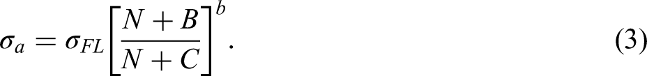

σ_{a} = σ_{F L} {[\frac{N + B}{N + C}]}^{b} .

(3)

Since B and C are not affected in Eq. (3), the modification of the curve in the fatigue limit parameter must be accompanied by modifying also the exponent parameter from b to b_k: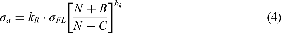

σ_{a} = k_{R} \cdot σ_{F L} {[\frac{N + B}{N + C}]}^{b_{k}}

(4)

If both formulas Eq. (3) and Eq. (4) are compared at the tensile strength (N = 0), it can be proven that: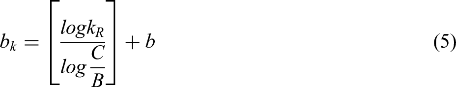

b_{k} = [\frac{l o g k_{R}}{l o g \frac{C}{B}}] + b

(5)

In the case of the application here in this study, the specimens relate to the bottom curve in Figure 9, i.e., the fatigue limit derived from K&V approximations in Figure 7 and Figure 8 equals to k_R·σ_FL, and the idealized fatigue limit must be derived from it by dividing its value by k_R coefficient. As its values vary between 0.85 and 0.92, this moves all curves at the bottom asymptote upwards, see Figure 10, while the slope coefficient b of the polished fatigue curves must be computed from the b_k coefficient related to the experimental data (Table 8, Table 9).

Figure 10.

(left) K&V regression curves of all series with parameters stated in Table 8 and Table 9, (right) corrections of K&V curves with respect to measured roughness values via Eq. (4)

Figure 10 illustrates the Kohout–Věchet S-N curves, if the modification introduced in Eqs. (2)-(5) was applied, though deployed on a limited range of experimental data. Though the Kohout-Věchet curve allows the transition of the trend to horizontal asymptotes in the quasi-static or fatigue limit domains, this change of the trend is usually driven by few outmost-lying specimens. Because the coverage by experiments in these areas is usually insufficient, these plots are not intended for evaluating the trends in those plateaus but for evaluating the change in the mutual positions of curves in their interpolated domains.

Though the final S-N curves in Figure 10 (right) relate to the same Rz of 1μm, they are still affected by differing residual stresses, which means they cannot be directly compared each to other. To see, if there is any trend in the response in fatigue life to the imposed residual stress, the relation between the obtained fatigue strength at 1 million cycles for modified and non-modified S-N curves from Figure 10 and the measured residual stresses is depicted in Figure 11. It is based on a commonly accepted assumption that the residual stresses act similarly to mean stresses of fatigue cycles. The fatigue strength at 1 million cycle is chosen instead of the comparison of σ_FL values. Derived fatigue limits are too affected by a limited number of specimens defining the fatigue curve in the fatigue limit region (as mentioned for A35).

Figure 11.

Relationship between axial (top) and tangential (bottom) residual stresses with respect to the fatigue strengths related to 1,000,000 cycles: (left) from experiment, (right) corrected to reflect roughness

Figure 11 shows that a specific trend similar to the Haigh diagram can be traced in a limited way only: both graphs show decrease of the allowable stress amplitude with increasing mean stress. The data points remain rather scattered in both graphs (before the roughness-based modification and after applying it). It is true that the scatter of the data points from linear trends decreases after the roughness modification is introduced, but the improvement is only mild. This is the obvious proof that the already mentioned suspicion of another relevant and unaccounted parameter in the study can be realistic. The mentioned micro-notch artefact and the abrupt changes in the residual stress distribution along the longitudinal direction (see Figure 6) is one of the potential reasons, because at distances of tenths of a millimeter, the detected levels of residual stresses may vary. However, based on the course of Figure 6 and the difference in residual stress values in Table 7, it can be argued that the influence of the notch is smaller than the absolute differences between the individual series.

Correlation matrix

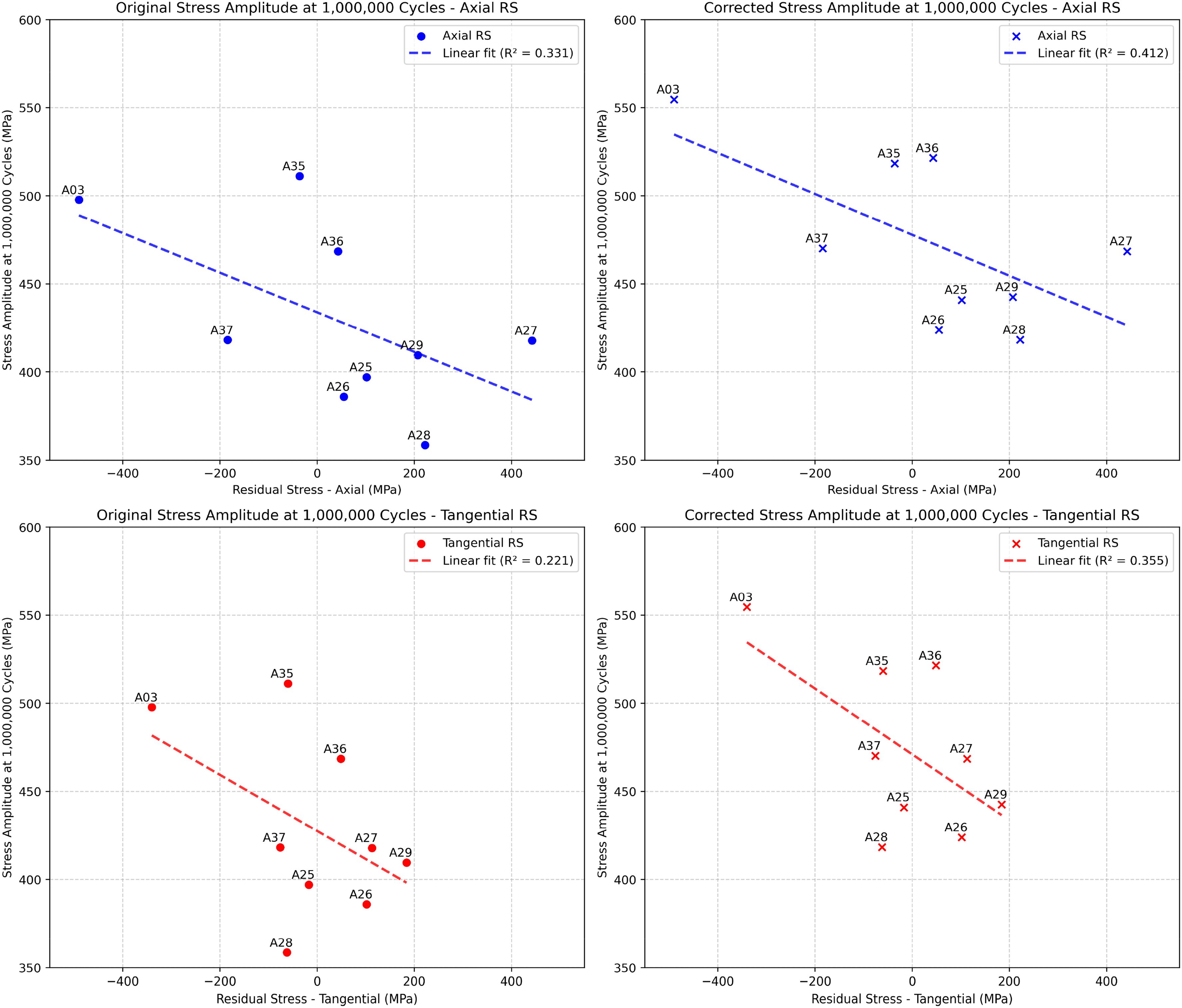
Determining the exact contribution of each parameter to a specific outcome is challenging. In the following section, a simplified correlation matrix ( Figure 12) that examines the relationship between turning parameters Table 3 (binary 1 for yes and 0 for no as regards the cooling) and key outcomes is presented. These include surface roughness (Ra, considering only the mean value measured at CTU), residual stresses (both axial and tangential), and fatigue strength at 1,000,000 cycles from regression curves, parameter of which are in Table 8 and Table 9.

Figure 12.

Correlation matrix of input parameters of turning and outcoming results with display of Person correlation coefficient^48,49 and highlighted contour

The correlation matrix Figure 12 provides insights into the relationships between machining parameters and fatigue life outcomes. Using the conventional approach for interpreting Pearson's correlation coefficient, we can analyze the strength and significance of these relationships. The evaluation was performed as suggested by Schober et al.,⁵⁰ although the correlation coefficient can be interpreted differently.⁵¹ Schober et al.⁵⁰ outlines a conventional approach to interpreting correlation coefficients, where a value between 0.00–0.10 indicates a negligible correlation, 0.10–0.39 a weak correlation, 0.40–0.69 a moderate correlation, 0.70–0.89 a strong correlation, and 0.90–1.00 a very strong correlation. The same absolute values but with the minus sign show a similar level correlation but in the opposite trend, when increase in a parameter value leads to decrease in a value of the other parameter.

Some of the key detected dependencies are also highlighted separately in Figure 13.

Figure 13.

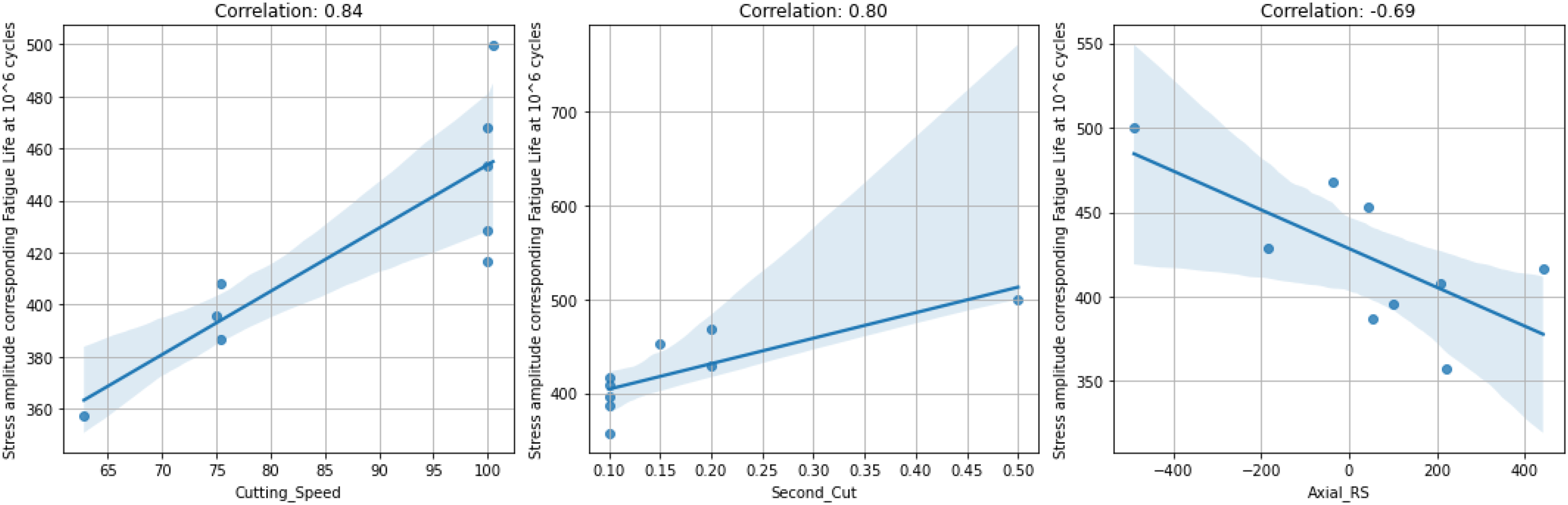
Strong correlation coefficients between cutting speed, the second-to-last cut, and residual stresses in axial direction with stress amplitude, as related to fatigue life at 1,000,000 cycles. The shaded area represents the 95% confidence interval (CI), indicating the range where the true regression line is likely to fall

Cutting speed (from 62.5 to 100 m/min): The correlation matrix shows its utmost importance in delivering specimens with a good fatigue strength. The higher cutting speed (within limits evaluated here), the better fatigue performance was obtained. On the other hand, its effect on other observed parameters (residual stresses or roughness) is rather weak (though not negligible).

Feed rate (either 0.05 or 0.1 mm): Somewhat surprisingly to our team, practically no correlation with any observed parameter was found. This outcome could be caused either by a limited range of evaluated values, and/or other inputs hiding its effect.

Last cut height (either 0.05 or 0.1 mm): A weak correlation with fatigue strength is detected, where the deeper cuts led to higher fatigue strength. A more prominent is the trend of decreasing roughness with increasing last cut height, which is observed despite low variability of the input parameter. Both trends are showing that the attempt to improve properties by decreasing the cut height is ineffective and the cut height of 0.05 mm causes rather harm, probably due to worse chip formation or possibility of occasional sliding of the tool over the specimen surface.

Second last cut height (from 0.1 mm to 0.5 mm): Only one setup was tested with the height of 0.5 mm (A03) and the rest of cases was within narrower range between 0.1 and 0.2 mm. Thanks to the higher variability of the input however, the correlation of observed parameter with the second cut height is much stronger than in any other cases here. The bigger is this height, the lower are both residual stress parameters and also the fatigue strength increases. The relation between both observed parameters is already documented in Figure 11 and complies to the expectations of the Haigh diagram.

What surprises however is the effect of the second last cut height on any of these observed parameters. The minimum applied last cut height was 0.05 mm in any case. Within FABER project, multiple attempts to observe also the residual stress profile into the depth were made (but none related to the series described here, and thus the graphs are not reported here), and in all cases the residual stresses diminished practically to zero at 40–60 microns. The last cut should remove them completely, and its effect on the roughness level after the second last cut is also obvious. This means that the detected dependency is very likely caused by the single value of 0.5 mm in A03 which led to superior fatigue strengths, while the improved Ra roughness relates to the only case of grinding the surface. The extreme broadening of the confidence interval in Figure 13 is another symptom of the uncertainty related to the only item with high second last cut in the set.

Use of cooling (yes vs no): As expected, the use of cooling decreases residual stresses to some extent and positively affects the fatigue strength. Its negligible influence on roughness is also in line with general expectations.

Ra roughness effect (0.6–1.8 μm): Decrease of roughness correlates with increase of fatigue strength. A moderate positive correlation was however found also to the axial residual stress, while the correlation to the tangential residual stress is practically zero.

Residual stresses: Both axial and tangential residual stress parameters are mutually strongly correlated. It is not surprising at all that the lower they are the higher is the fatigue strength, which is clearly documented also in Figure 11.

Some of the above-mentioned observations are far from being surprising (the effect of residual stresses, the impact of cooling on residual stresses only or increase of fatigue strength with decreased roughness). The analysis of the effect of process parameters brings along some interesting points – the very minor effect of the feed rate or the last cut height effect, which favors rather 0.1 mm than 0.05 mm. It can be only speculated, whether the possible clearance that could cause the single artefact reported in Sec. 3c, could also affect this performance, and whether a newer CNC machine would result in the same outcome.

Conclusion

This study demonstrates the significant impact of machining parameters on fatigue performance in 42CrMo4 + QT steel specimens, revealing substantial variations in fatigue strength ranging from 360 MPa to 510 MPa at 1 million cycles. The correlation analysis provides some insights into the relationships between machining parameters and fatigue life, with cutting speed showing a strong positive correlation with fatigue life across different cycle ranges. The depth of second last cut demonstrated strong positive correlations with fatigue strength at 1 million cycles, but it is explained in the paper that this is rather an outcome of an iterative search for better performing setups of machining parameters, while the systematic design of experiments process would result in other conclusions.

While surface roughness and residual stresses are important factors, their relationship with fatigue strength is more complex than previously assumed. Surface roughness shows a moderate negative correlation with fatigue strength at 1 million cycles, while axial and tangential residual stresses demonstrate moderate-to-strong negative correlations. Notably, these surface measurements alone prove insufficient as reliable predictors of overall fatigue performance, despite their common use in manufacturing inspection.

To better account for the effects of surface roughness on fatigue performance, we propose a modification of the Kohout-Věchet (K&V) model by introducing a roughness correction coefficient based on FKM-Guideline formula. This adjustment allows for a more accurate estimation of fatigue limits based on surface conditions and provides an improved predictive capability for high-cycle fatigue behaviour. The correction successfully aligns fatigue life predictions across different machining configurations, reducing data scatter and offering a refined approach to fatigue analysis.

The confrontation of the results of the roughness correction in a graph similar to Haigh diagram shows that the scatter in available data remains excessive, proposing that some non-included effect induces it. Two potential reasons are proposed:

The micro-notch of 10 microns height along approximately 0.4 mm length of the specimen in its central section is observed on all specimens, irrespective which manufacturing setup was used. It probably originates from a clearance in tool-machine connection. It does not represent only surface defect, but a study on another high-strength steel documents in Figure 6, that it causes changes in residual stress distribution along the specimen axis.

The residual stress information from XRD only on the surface need not be sufficient to relate the effect of machining parameters on the fatigue life of specimens. The residual stress profile into the depth could show more (and also to confirm the assumption that the importance of the second last cut height highlighted in the Pearson correlation matrix is not real but induced by the selection of the test cases.

These items can highlight to next researchers where to focus their attention so that they do not repeat our mistakes and improve the monitoring of parameters relevant to the final fatigue life. The practical challenge remains that these more complex characteristics are difficult to measure in typical post-production quality control settings. Consequently, conservative design approaches must currently rely on the lowest observed fatigue strength values, unable to utilize the substantial potential performance margin (nearly 50% higher) until new parameters or measurement methods are developed. This work provides valuable insights for both researchers and industrial practitioners, highlighting how specific machining parameters, particularly cutting speed and final cut depths, can affect the fatigue performance while emphasizing the need for further research into currently unexamined factors affecting fatigue life in high-strength steels.

Footnotes

Nomenclature

Acknowledgements

The financial support provided by the Czech Science Foundation within the 23-06130K project and by the Grant Agency of the Czech Technical University in Prague within the SGS23/156/OHK2/3T/12 and SGS25/168/OHK4/3T/14 projects is gratefully acknowledged. Tomáš Vrbata is acknowledged for his help with measurements of roughness in Mondragon.

ORCID iDs

Martin Matušů

Jan Papuga

Karel Trojan

Antonín Trefil

Alaitz Zabala

Vladimír Mára

Petr David

Ethical approval and informed consent statements

Ethical approval was not required for this study.

Author contribution(s)

Martin Matušů: Investigation; Methodology; Visualization; Writing – original draft; Writing – review & editing.

Jan Papuga: Conceptualization; Data curation; Formal analysis; Investigation; Methodology; Resources; Visualization; Writing – original draft; Writing – review & editing.

Karel Trojan: Investigation; Writing – review & editing.

Antonín Trefil: Formal analysis; Investigation; Resources; Writing – review & editing.

Alaitz Zabala: Investigation; Writing – review & editing.

Vladimír Mára: Investigation; Visualization; Writing – review & editing.

Petr David: Investigation; Visualization; Writing – original draft; Writing – review & editing.

Funding

The authors disclosed receipt of the following financial support for the research, authorship, and/or publication of this article: This work was supported by the České Vysoké Učení Technické v Praze, Grantová Agentura České Republiky, (grant number SGS23/156/OHK2/3T/12, 23-06130K).

Declaration of conflicting interests

The authors declared no potential conflicts of interest with respect to the research, authorship, and/or publication of this article.

Data availability

Data will be made available on request.

Declaration of generative Ai and Ai-assisted technologies in the writing process

During the preparation of this work the author(s) used OpenAI Chat GPT in order to improve clarity and readability. After using this tool/service, the author(s) reviewed and edited the content as needed and take(s) full responsibility for the content of the publication.

References

Rennert

Vormwald

Esderts

. FKM-guideline “Analytical strength Assessment” – Background and current developments. Int J Fatigue 2024; 182: 108165. https://doi.org/10.1016/j.ijfatigue.2024.108165.

Rennert

. FKM-Richtlinie – Rechnerischer Festigkeitsnachweis für Maschinenbauteile. 6th rev. ed. Frankfurt am Main: VDMA Verlag GmbH, 2012.

Malakondaiah

Srinivas

Rao

. Ultrahigh-strength low-alloy steels with enhanced fracture toughness. Prog Mater Sci 1997; 42: 209–242. https://doi.org/10.1016/S0079-6425(97)00016-9.

Tümer

Schneider-Bröskamp

Enzinger

. Fusion welding of ultra-high strength structural steels – A review. J Manuf Process 2022; 82: 203–229.

Pyttel

Schwerdt

Berger

. Very high cycle fatigue – is there a fatigue limit? Int J Fatigue 2011; 33: 49–58.

Sonsino

. Course of SN-curves especially in the high-cycle fatigue regime with regard to component design and safety. Int J Fatigue 2007; 29: 2246–2258.

Okuda

Ogawa

Ichikawa

, et al. Influence of microstructure on fatigue property of ultra high-strength steels. Frattura ed Integrità Strutturale 2019; 13(48): 125–134. https://doi.org/10.3221/IGF-ESIS.48.15 .

Singh

Rao

. A surface roughness prediction model for hard turning process. The International Journal of Advanced Manufacturing Technology 2007; 32: 1115–1124.

Ozel

Hsu

Zeren

. Effects of cutting edge geometry, workpiece hardness, feed rate and cutting speed on surface roughness and forces in finish turning of hardened AISI H13 steel. The International Journal of Advanced Manufacturing Technology 2005; 25: 262–269.

10.

Zare Chavoshi

Tajdari

. Surface roughness modelling in hard turning operation of AISI 4140 using CBN cutting tool. IntJ Mater Form 2010; 3: 233–239.

11.

Eglin steel—a low alloy high strength composition, n.d.

12.

Tian

Jiang

. Exploring new strategies for ultrahigh strength steel via tailoring the precipitates. Frontiers in Materials 2021; 8: 1–7. https://doi.org/10.3389/fmats.2021.797798 .

13.

Chaouch

Guessasma

Sadok

. Finite element simulation coupled to optimisation stochastic process to assess the effect of heat treatment on the mechanical properties of 42CrMo4 steel. Mater Des 2012; 34: 679–684.

14.

Nesládek

Marcell Enzveiler Marques

Papuga

, et al. Fretting fatigue of 42CrMo4 QT steel: Experimental and numerical assessment. Int J Fatigue 2024; 189: 108575. https://doi.org/10.1016/j.ijfatigue.2024.108575.

15.

Nesládek

Matušů

Karas

, et al. Application of self-heating method to estimate fatigue limit of 42CrMo4 + QT steel under fretting fatigue conditions. Procedia Structural Integrity 2025; 68: 527–533. https://doi.org/10.1016/j.prostr.2025.06.092.

16.

Kumar

Aggarwal

Khokhar

. Difficulty in welding & effect of pwht on low alloy steel 42CrMo4 (EN19) using smaw process. International Journal of Scientific Development and Research 2024; 9(8): 252–261.

17.

Zhang

Wang

Liu

, et al. Surface Modification of 42CrMo Steels: A Review from Wear and Corrosion Resistance. Coatings 2024; 14(3): 337. https://doi.org/10.3390/coatings14030337.

18.

Morsy

El-Kashif

. Repair welding reclamation of 42CrMo4 and C45 steels: Green Welding Technologies for Effective and Reliable Manufacturing. In: Proceedings of IIW 2017 International Conference, Shanghai, China, June, 29-30, 2017. 2017. 1. vyd. Shanghai.

19.

Chen

Liu

Wang

, et al. Effect of surface integrity on fatigue life of 2024 aluminum alloy subjected to turning. J Manuf Process 2022; 83: 650–666. https://doi.org/10.1016/j.jmapro.2022.07.070 .

20.

Asiltürk

Akkuş

. Determining the effect of cutting parameters on surface roughness in hard turning using the Taguchi method. Measurement ( Mahwah N J) 2011; 44(9): 1697–1704. https://doi.org/10.1016/j.measurement.2011.07.003.

21.

Hamada

Ali

Ghosh

, et al. Comparative Study of High-Cycle Fatigue and Failure Mechanisms in Ultrahigh-Strength CrNiMoWMnV Low-Alloy Steels. Metals (Basel) 2024; 14: 1238. https://doi.org/10.3390/met14111238.

22.

Díaz-Salamanca

Muñiz-Calvente

Ebrahimzadeh

, et al. Influence of turning parameters on residual stresses and roughness of 42CrMo4 QT. The International Journal of Advanced Manufacturing Technology 2024; 134: 2897–2919. https://doi.org/10.1007/s00170-024-14257-5 .

23.

Özdemir

Kaya

Akyildiz

. Analysis of surface roughness and cutting forces in hard turning of 42CrMo4 steel using taguchi and RSM method. Mechanics 2020; 26: 231–241.

24.

Bouacha

Yallese

Mabrouki

, et al. Statistical analysis of surface roughness and cutting forces using response surface methodology in hard turning of AISI 52100 bearing steel with CBN tool. Int J Refract Met Hard Mater 2010; 28: 349–361.

25.

Suresh

Basavarajappa

Gaitonde

, et al. Machinability investigations on hardened AISI 4340 steel using coated carbide insert. Int J Refract Met Hard Mater 2012; 33: 75–86.

26.

Nabil

Zahia

Yalles

, et al. Statistical analysis of surface roughness by design of experiments in hard turning. Mechanika 2012; 18: 605–611.

27.

Gorlenko

. Assessment of surface roughness parameters and their interdependence. Prec Eng 1981; 3: 105–108.

28.

Papuga

Mžourek

Matušů

, et al. Investigation of the size effect on 42CrMo4 QT steel in the high-cycle fatigue domain part I: Experimental campaign. Int J Fatigue 2023; 175: 107743. https://doi.org/10.1016/j.ijfatigue.2023.107743.

29.

Matušů

Papuga

Mžourek

. Fatigue strength estimation of 42CrMo4 QT from the temperature evolution during cyclic loading. Procedia Structural Integrity 2022; 42: 102–109.

30.

Matušů

Papuga

. Prediction of fatigue life of 42CrMo4 + QT steel using self-heating effect. 62nd Annual Conference on Experimental Stress Analysis n.d.; 62: 12.

31.

FABER (Fatigue Benchmark Repository). 2020. https://www.pragtic.com/faber.php#fabest (accessed 2025-01-30).

32.

Meneghetti

. Analysis of the fatigue strength of a stainless steel based on the energy dissipation. Int J Fatigue 2007; 29: 81–94.

33.

Matušů

Šimota

Papuga

, et al. S–N curves established from limiting energy in the case of specimens additively manufactured from AlSi10Mg. Fatigue & Fracture of Engineering Materials & Structures n.d.; 47(12): 4771–4790. https://doi.org/10.1111/ffe.14442.

34.

Wang

Crupi

Jiang

, et al. Energy-based approach for fatigue life prediction of pure copper. Int J Fatigue 2017; 104: 243–250.

35.

Chen

. Cutting forces and surface finish when machining medium hardness steel using CBN tools. Int J Mach Tools Manuf 2000; 40: 455–466.

36.

Allenov

Borisovna

Ghorbani

, et al. Simultaneous effects of cutting depth and tool overhang on the vibration behavior of cutting tool and high-cycle fatigue behavior of product: experimental research on the turning machine. The International Journal of Advanced Manufacturing Technology 2022; 122: 2361–2378.

37.

Hadi

Ahmed

. Assessment of surface roughness model for turning process. In: Wang

Kovacs

Wozny

Fang

(eds) Knowledge enterprise: intelligent strategies in product design, manufacturing, and management. Boston, MA: Springer US, 2006, pp.152–158. https://doi.org/10.1007/0-387-34403-9_19 .

38.

Özdemir

. Optimization with taguchi method of influences on surface roughness of cutting parameters in CNC turning processing. Mechanics 2019; 25: 397–405.

39.

E466 − 21 Standard Practice for Conducting Force Controlled Constant Amplitude Axial Fatigue Tests of Metallic Materials n.d.

40.

ISO 1099:2017 Metallic materials — Fatigue testing — Axial force-controlled method 2017.

41.

Zielinski

Vovk

Riemer

, et al. An Investigation on Internal Material Loads and Modifications in Precision Turning of Steel 42CrMo4. Micromachines (Basel) 2021; 12: 526. https://doi.org/10.3390/mi12050526.

42.

Čapek

Kec

Trojan

, et al. Fatigue Properties and Residual Stresses of Laser-Welded Heat-Resistant Pressure Vessel Steel. Verification on Vessel Model. Metals 2022; 12(9): 1517. https://doi.org/10.3390/met12091517.

43.

Čapek

Trojan

Kec

, et al. Residual Stresses and the Microstructure of Modeled Laser-Hardened Railway Axle Seats under Fatigue. Metals (Basel) 2024; 14(3): 290. https://doi.org/10.3390/met14030290.

44.

ČSN EN ISO 683-17 Heat-treatable steels, alloy steels and free-cutting steels – Part 17: Ball and roller bearing steels 2024.

45.

Marques

Mžourek

Papuga

, et al. A probabilistic stress-life model supported by weakest link principle and highly-stressed volume/surface area concepts. Int J Fatigue 2024; 178: 108006. https://doi.org/10.1016/j.ijfatigue.2023.108006.

46.

Kohout

Věchet

. A new function for fatigue curves characterization and its multiple merits. Int J Fatigue 2001; 23: 175–183.

47.

Marques

Papuga

Růžička

, et al. A probabilistic fatigue model based on nonlinear Kohout-Věchet function: Application to 42CrMo4 QT steel. J Phys: Conf Ser 2024; 2692: 012032. https://doi.org/10.1088/1742-6596/2692/1/012032.

48.

Asuero

Sayago

González

. The correlation coefficient: an overview. Crit Rev Anal Chem 2007; 36: 41–59.

49.

Kirch

. Pearson’s correlation coefficient. In: Kirch

(eds) Encyclopedia of public health. Dordrecht: Springer Netherlands, 2008, pp.1090–1091. https://doi.org/10.1007/978-1-4020-5614-7_2569 .

50.

Schober

Boer

Schwarte

. Correlation coefficients: appropriate use and interpretation. Anesth Analg 2018; 126: 1763–1768.

51.

Akoglu

. User's guide to correlation coefficients. Turkish Journal of Emergency Medicine 2018; 18: 91–93.