Sage Journals: Discover world-class research

Abstract

Microstructural defects are commonly found in additively manufactured materials and can have significant effects on the material's bulk properties. This warrants defect detection and classification during microstructural evaluation, which is often laborious, costly, and can yield sub-optimal results if done manually. Previous attempts to facilitate automated classification in additively manufactured nickel-alloys have used supervised machine learning methods, such as kth-nearest neighbour classification and decision trees. This study proposes and evaluates the use of convolutional neural networks for microstructural defect classification in selective laser melted Inconel 713C samples. It outlines the process used to create, augment and expand the dataset, as well as hyperparameter selection for the neural network architecture to yield optimal classification performance.

Keywords

additive manufacturing nickel alloys microstructural defects machine learning deep learning

Introduction

Additive manufacturing (AM) is a class of manufacturing processes, that enables the creation of components, layer-by-layer using a high-energy heat source, from three-dimensional models. The characteristics of AM lead to various advantages when compared to traditional manufacturing processes. For instance, AM enables the production of intricately complex parts with enhanced design flexibility, optimises structural topology to improve mechanical properties, consolidates multiple components into single units to reduce weight and cost, and supports on-demand production, collectively enhancing efficiency, cost-effectiveness, and environmental sustainability.^1–3 While these advantages are significant, further exploration is needed to deepen our understanding of the “process-microstructure-property” relationship in AM, which would enhance the design and optimisation of materials and manufacturing processes.⁴ Components produced using AM methods are typically prone to the presence of microstructural defects, such as lack of fusion defects, gas porosities, solidification cracking and keyhole collapses, which pose risks in structural applications, especially when under cyclic loading conditions.^5,6 For these reasons, studying the “process-microstructure-property” relationship is vital to advancing the performance of engineering components. An essential part of the investigation of this relationship is correctly detecting and classifying microstructural defects from microstructural images. However, when performed manually, the detection and classification of microstructural defects can often be laborious, costly and yield suboptimal results, suggesting the need for an alternative strategy to detection and classification.⁷

Machine Learning (ML) is a branch of Artificial Intelligence that offers a solution to data analysis in the field of materials science. It focuses on pattern identification and cognitive acquisition concepts, which optimise performance criteria based on example data or past experiences.^8,9 In the field of AM, supervised and unsupervised machine learning methods have been used for a variety of microstructural detection and classification applications. For instance, unsupervised learning has been used to classify gas pores, keyhole pores resulting from excessive energy input, and lack of fusion pores caused by insufficient energy input.¹⁰ Unsupervised machine learning has been employed to identify and classify anomalies in a laser powder bed additive manufacturing process using a moderately-sized training database of image patches.¹¹ K-means clustering, a supervised ML model, and support vector machines, a unsupervised ML model, have been used to detect porosities in thin-walled aluminium alloy structures with an average classification accuracy of 99%.¹²

Deep Learning, another subset of ML algorithms, has been pivotal in advancing the state-of-the-art across various domains, including speech and visual object detection and classification.^13,14 Deep Learning algorithms are better at learning complicated patterns from more complex datasets, leading to their increased use in materials science applications. For instance, it has been used to distinguish between metallic morphologies with dendrites and those without.¹⁵ It has also been used for lath-bainite segmentation in complex-phase steel, achieving an accuracy of 90% which rivals the accuracy of expert segmentations.¹⁶ Deep learning has also found use in the design of new materials and to link microstructural characteristics to the material's bulk properties.^17,18 For an overview on the previous use of deep learning approaches in microstructural characterisation, the reader is directed to these resources for more information.^16,19 In particular for AM, Deep Learning has been used to enhance process monitoring and quality identification by automatically analysing image data of manufactured parts with Convolutional Neural Networks (CNNs).²⁰ Graph autoencoders with graph convolutional networks have been used to analyse and design micro lattice architectures by mapping structures to mechanical properties and reconstructing designs based on desired properties.²¹ Finally, PyroNet, a CNN-based model, and IRNet, a Long-term Recurrent Convolutional Network-based model, have been used for in-situ porosity detection in laser-based AM, fusing predictions from both networks for improved accuracy.²² For more information on the applications of deep learning in additive manufacturing, the reader is directed to the following articles.^23,24

This paper builds on the work of Aziz et al. who used k-th Nearest Neighbours (kNN) and decision tree algorithms to classify defects found in a variety of nickel-alloys with 89.8% and 90–92% accuracy respectively.²⁵ In this study, CNNs are used to automatically classify the different types of defects that are present in Inconel 713C alloy. It will outline the process to sourcing binary images of individual defects from micrographs of the alloy samples, the preprocessing that the dataset underwent, as well as the methodologies used for CNN optimisation including hyperparameter tuning and data augmentation. It will then evaluate the efficacy of neural networks as a method to classifying defects, comparing the network's performance to that of the supervised machine learning methods used by Aziz. et al.²⁵

Methodology

Dataset creation and preparation

A range of micrographs of the Inconel 713C alloy samples were produced using selective laser melting during a research program at the University of Sheffield, with varying settings for power, beam velocity and hatch spacing.²⁶ The micrographs, an example of which is shown in Figure 1, were then imported into MATLAB and converted into a binary image, clearly showing the microstructural defects. The scale, shown on the bottom, along with defects that intersected the border of the micrograph were removed, to ensure the quality of the dataset. In addition, defects that were too small (below 10 pixels in area), were excluded as low-resolution images made manual classification challenging. After filtering unwanted data, individual binary images of the defects in the micrographs were created, as illustrated in Figure 1. The images were categorised into specific classes: ‘crack’, ‘pore’, ‘lack of fusion’, and ‘pore with crack’ defects. This process was applied to the 18 micrographs, yielding a dataset of 4800 binary images of microstructural defects. In this dataset, there were 1807 ‘crack’ defects, 900 ‘lack of fusion’ defects, 1830 ‘pore’ defects, and 263 ‘pore with crack’ defects.

Figure 1.

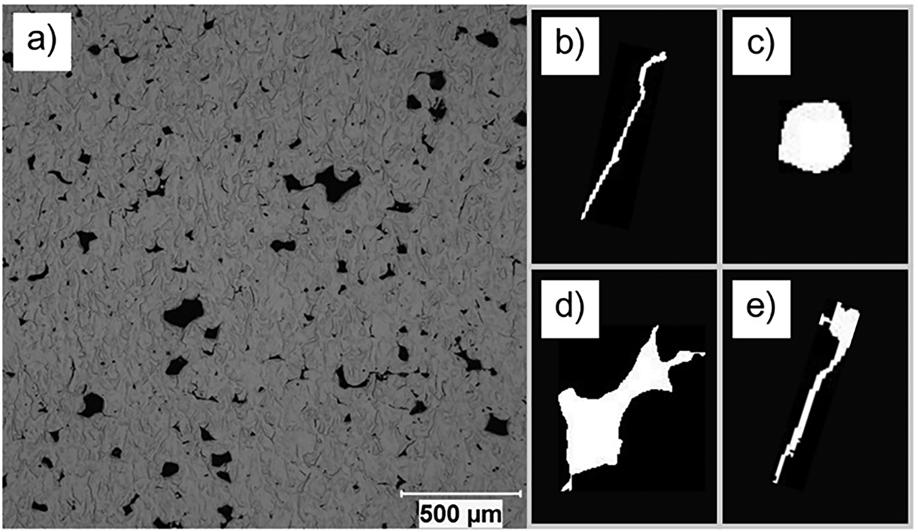
Example micrograph used to create the dataset, with example binary images of each defect type that were found in the micrographs. This includes (b) ‘crack’, (c) ‘pore’, (d) ‘lack of fusion, and (e) ‘pore with crack’ defects.

Data augmentation

The defect dataset images were standardised to a size of 200 × 200 pixels. It should be noted that resizing images can lead to some loss or distortion of the original information, as shrinking an image may lead to loss of detail, and enlarging an image may lead to pixelation.²⁷ This may affect the accuracy of subsequent image analysis or ML models that rely on high-quality data. Data augmentation was also applied to the dataset. Deep learning models typically demand extensive datasets to gather sufficient information and patterns for effective training and performance. Data augmentation can support with mitigating overfitting to training data, which would result in the model's poor generalisation performance on unseen samples.^28,29 In this work, augmentation involved a random reflection on the X and Y axis of the image, a random rotation of the image from 20 to −20 degrees around its centre, and a random scaling of 0.9 to 1.1. Following augmentation, the dataset was compiled into a training dataset (70%) and a validation dataset (30%).

Baseline model

To begin, a baseline neural network was created as a foundational model for optimisation. It used a filter size of 5 × 5 which was kept consistent for all subsequent model training. The baseline model consisted of 4 blocks and 10 filters per block. Each block is of a standard architecture, containing a two-dimensional (2d) convolution layer, batch normalisation layer, rectified linear unit (ReLU) layer and a max pooling layer as shown in Figure 2. 2d convolution layers apply convolution operations, where kernels (filters) slide over the input image to extract features such as edges, textures or patterns.³⁰ Batch normalisation layers stabilise and accelerates training by normalising activations from the previous layer in the network.³¹ ReLU layers are an activation function that introduce non-linearity into the model, enabling the CNN to learn more complex patterns from the input data,³² while max pooling layers downsample spatial dimensions to reduce computational cost and emphasise the most significant features.³³ By varying the number of blocks and ‘stacking’ them on top of each other, we achieve a network with different architectures, modifying its ability to learn the patterns from the training data and improving overall performance. For a more detailed description of Deep Learning and CNNs, the reader is directed to this textbook for more information.³⁴

Figure 2.

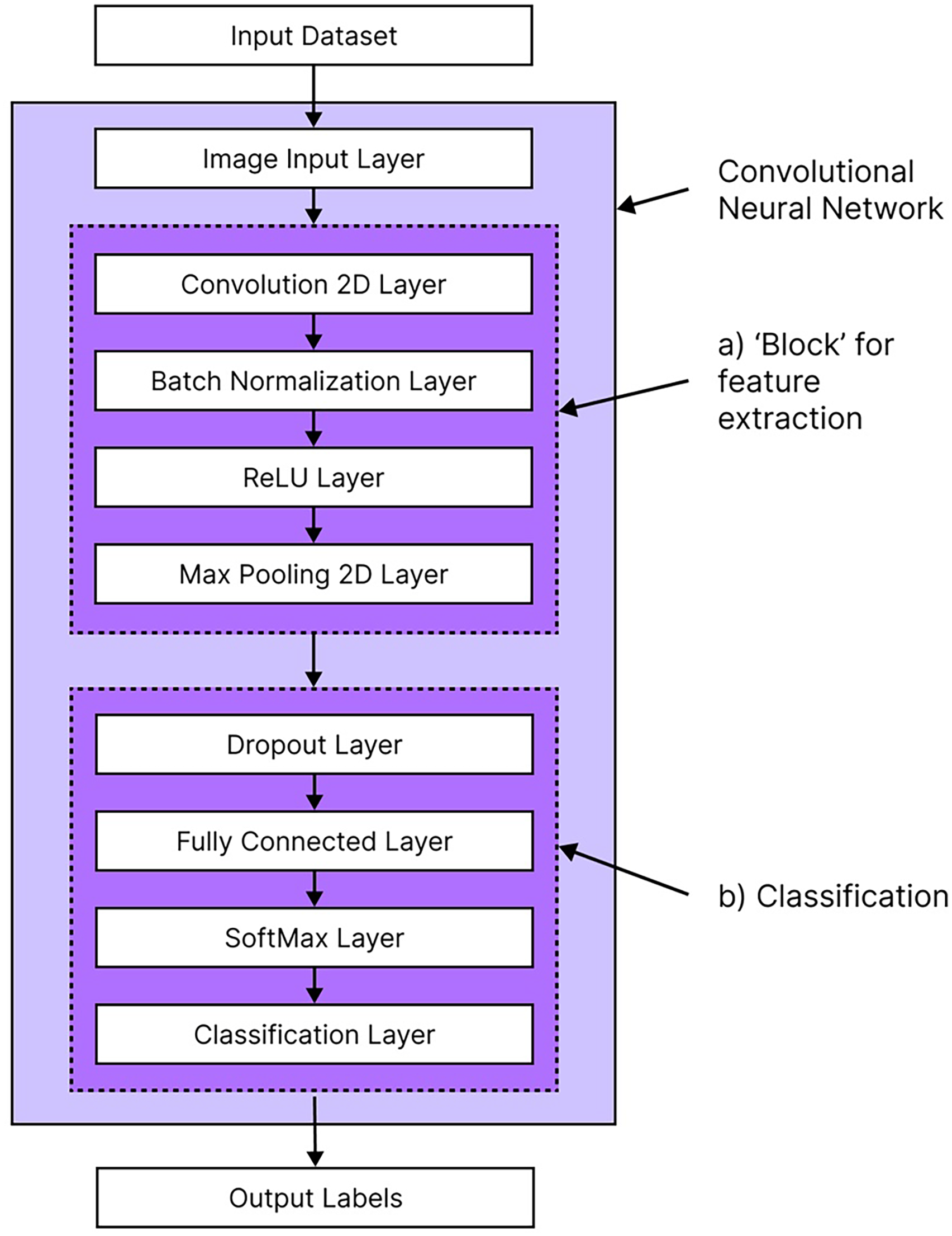
General structure of a convolutional neural network (CNN) highlighting (a) the feature extraction ‘blocks’ and (b) the classification layers for processing input datasets into output labels.

Hyperparameter tuning and optimisation

An important feature of designing and optimising neural networks is hyperparameter tuning.

In ML models, there are two types of parameters to consider: model parameters, which are initialised internally in the model and vary as the machine learning algorithm learns (such as weights of neurons in a neural network), and hyperparameters, which are freely selectable external parameters that do not vary while the model is learning.^35,36 In the context of neural networks, hyperparameters are settings that can be changed to influence the learning process (such as training time, learn rate, or batch size) and the architecture of the neural network (such as number and type of hidden layers and number of neurons).^37,38

Hyperparameter optimisation algorithms are useful because they enhance neural network performance by tailoring its architecture to the specific dataset and application, standardise comparisons between models, and reduce human effort required to explore possible combinations of hyperparameters.³⁶ In this work, two methods of hyperparameter optimisation were performed: (i) Grid-search and (ii) Bayesian optimisation.

Grid-search is a basic hyperparameter tuning method where a model is built using each combination of hyperparameters, trained, and then evaluated based on its performance.³⁹ In this grid-search, the number of blocks and filters in the CNN were explored, to evaluate which combination of these two CNN characteristics yields the optimal performance for microstructural defect classification. A disadvantage to grid search is that as the range of values being explored increases, the computational efficiency of the algorithm drastically decreases. To combat this, each model trained during grid search used 25% of the training dataset, improving computational efficiency of the algorithm. The optimal CNN architecture that yielded the optimal results in grid search was then trained with the full training dataset, to evaluate its performance on the full dataset and standardise training. During grid-search, CNN architectures with 2–7 blocks and 5–25 filters (with increments of 5) were explored.

Bayesian optimisation is a more advanced approach to hyperparameter optimisation. The algorithm builds a response surface model using the mean and uncertainty predictions to guide the selection of subsequent data collection.⁴⁰ It's ability to ‘learn’ from previous iterations makes it a more efficient approach to hyperparameter selection and Neural Architecture Search when compared to grid search.⁴¹ Due to this improvement compared to grid search, the scope of hyperparameters explored during optimisation was widened. This included varying the number of blocks, number of filters, initial learn rate, mini batch size, learn rate drop factor, and learn rate drop period.

Results and discussion

Original dataset

Confusion matrices describing the performance of the baseline model and models produced using optimisation methods are shown in Figure 3. Confusion matrices display the counts of actual versus predicted classifications provided by the model, with each cell in the matrix representing the frequency of predictions for each class, including both correct and incorrect predictions. Confusion matrices allow for the evaluation of overall model accuracy and assists with identifying the model's weaknesses when classifying certain types of defects. Table 1 presents the performance of each model in accurately classifying defects within the validation dataset along with its total accuracy. The network produced by gridsearch optimisation contained 7 blocks and 10 filters, whereas Bayesian optimisation yielded a model with 8 blocks and 26 filters. There was a steady increase in model classification performance as different optimisation methods were used to vary the hyperparameters of the model, with the Bayesian optimised model yielding the highest overall classification performance. This suggests that CNNs with more complex architectures yield better results, as they are better able to capture distinctive features between different types of microstructural defects, which has been found in prior research.^42,43

Figure 3.

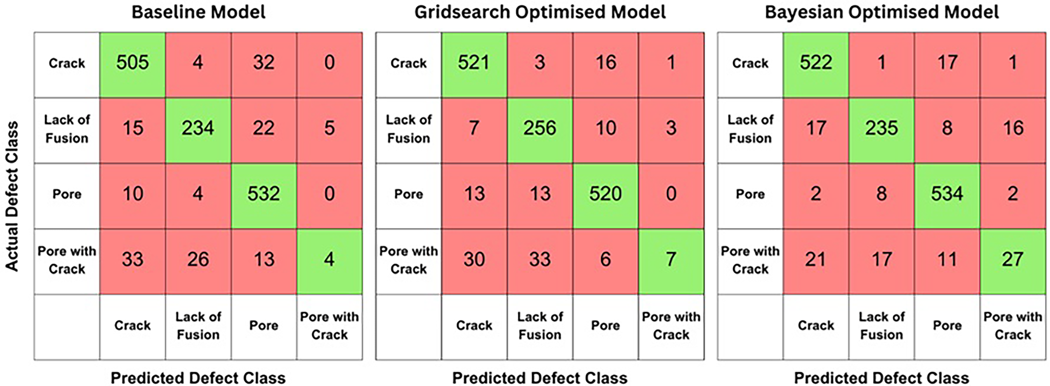
Confusion matrices showing the performance of the baseline, grid-search optimised, and Bayesian optimised models for classifying ‘crack’, ‘pore’, ‘lack of fusion’ and ‘pore with crack’ defects in the original dataset. The validation dataset consists of 1439 instances.

Table 1.

Summary of accuracy for baseline, grid-search optimised, and Bayesian optimised models in correctly classifying defects in the original dataset. The validation dataset consists of 1439 instances.

Defect Type	Baseline Model	Grid-search Optimised Model	Bayesian Optimised Model
Crack	93.3%	96.3%	96.5%
Lack of Fusion	84.8%	92.8%	85.1%
Pore	97.4%	95.2%	97.8%
Pore with Crack	5.3%	9.2%	35.5%
Total	88.6%	90.6%	91.6%

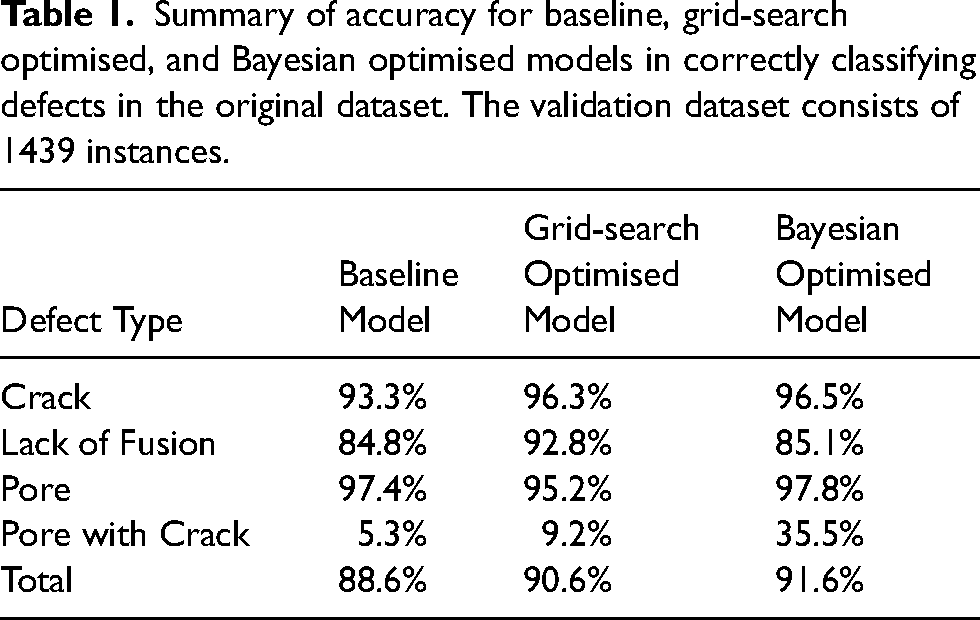
Similar to supervised ML models produced by Aziz et al.,²⁵ the CNNs faced consistent challenges in accurately classifying ‘pore with crack’ defects. These defects combine the characteristics of ‘pore’ and ‘crack’ defects, which already exist as separate classes in the dataset. The CNNs struggle due to overlapping features between these classes, making it difficult to distinguish and classify them effectively. ‘Pore with crack’ defects may overlap with ‘pore’ or ‘crack’ defects due to shared visual features such as round void shapes from pores and linear, sharp features from cracks. Moreover, this disparity could also stem from the imbalance in the dataset, where there were only 263 instances of ‘pore with crack’ defects out of a total of 4800 defects. This imbalance may suggest that the model is overfitting to the more prevalent defect types.^44,45

Despite it's poor performance in correctly classifying ‘pore with crack’ defects, the models showed strong capability at distinguishing between ‘lack of fusion’, ‘pore’ and ‘crack’ defects. The final model produced by Bayesian optimisation showed a overall performance of 91.6%, which is similar to that of models produced by Aziz et al.²⁵ It should be noted when compared to kNN classification and decision trees, the training and optimisation of CNNs for classification is significantly more time-consuming and computationally intensive. Moreover, the performance of the optimal models do vary each time the model is trained as shown in Figure 4. The variability observed in our model's performance across different training sessions shows the influence of factors such as initial weight settings,⁴⁶ data shuffling,⁴⁷ and hyperparameter choices.⁴⁸ The randomness in training neural networks highlights the importance of training models multiple times and reporting average performance metrics to ensure reliable and robust model performance, which is discussed further in Model evaluation and comparison. The overall accuracy of models produced by Bayesian optimisation is similar to that of deep learning models used for a variety of other applications in materials science, such as models that classify dendritic and non-dendritic microstructures and models that segment lath-bainite in complex-phase steel, which are both roughly 90% accurate.^15,16

Figure 4.

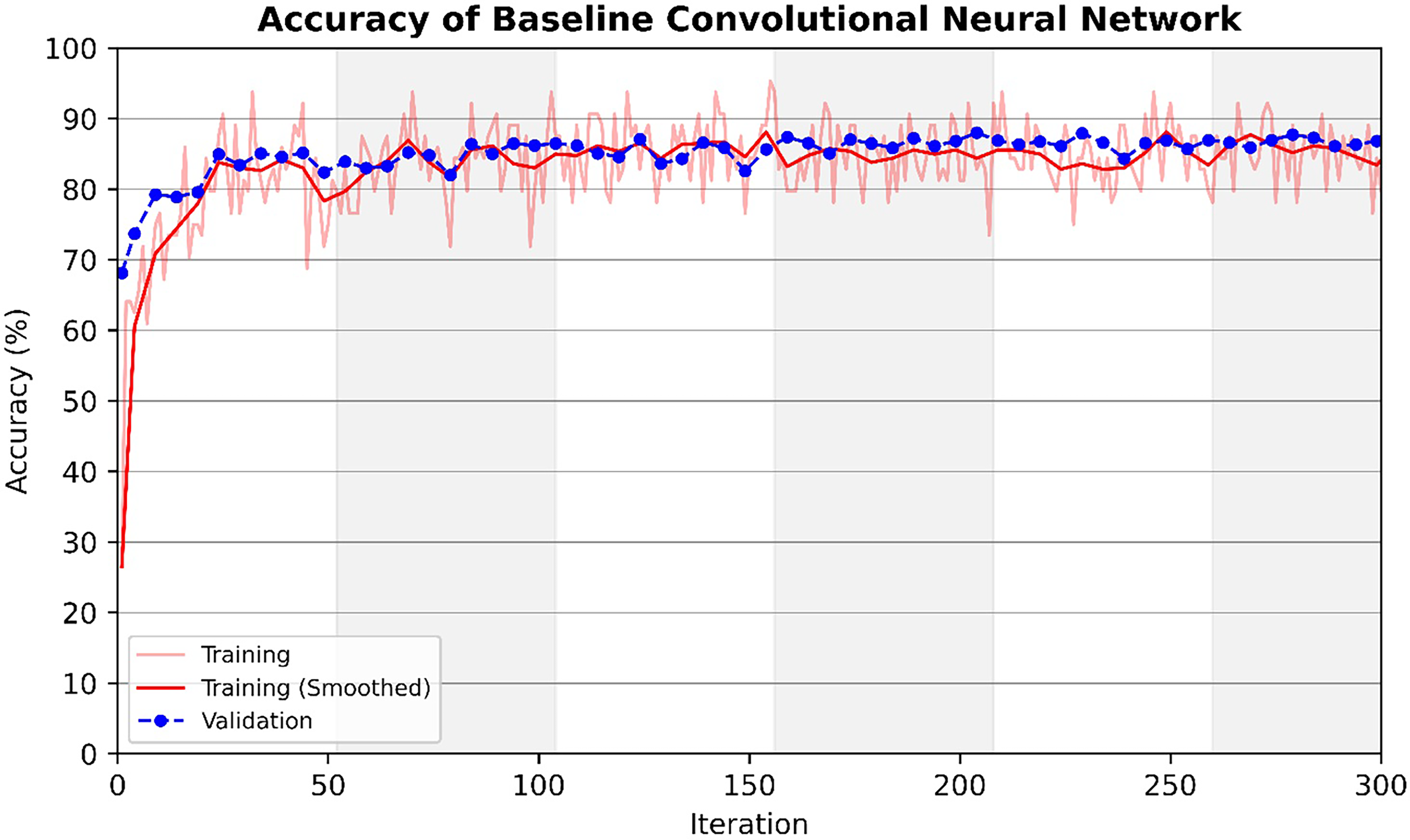
Variation in training accuracy and validation accuracy with number of training iterations for the baseline model (4 blocks and 10 filters) trained on the original dataset.

Synthetic dataset

To address the sub-optimal performance in classifying ‘pore with crack’ defects, the original dataset was expanded using data augmentation techniques to create a dataset containing ‘synthetic’ data. Data augmentation is a valuable tool in deep learning, enabling the expansion of datasets for improved training and validation.^49,50 In this study, the augmentation process included randomly reflecting the images along the X and Y axes, rotating the images between 20 and −20 degrees around their centre, and scaling the images randomly between 0.9 and 1.1. During augmentation, the ‘pore with crack’ defect class was expanded to 1052 instances – 4 times larger than the original size. After augmentation, the data was divided into a training set (70%) and a validation set (30%). The ‘crack’, ‘pore’ and ‘lack of fusion’ classes were not expanded as they were well classified in previous models. The baseline model was trained with 4 blocks and 10 filters. Grid-search optimisation identified the optimal network configuration with 8 blocks and 20 filters, while Bayesian optimisation yielded a CNN with 9 blocks and 28 filters. The confusion matrices for the models’ performance are provided in Figure 5, and their accuracies are shown in Table 2.

Figure 5.

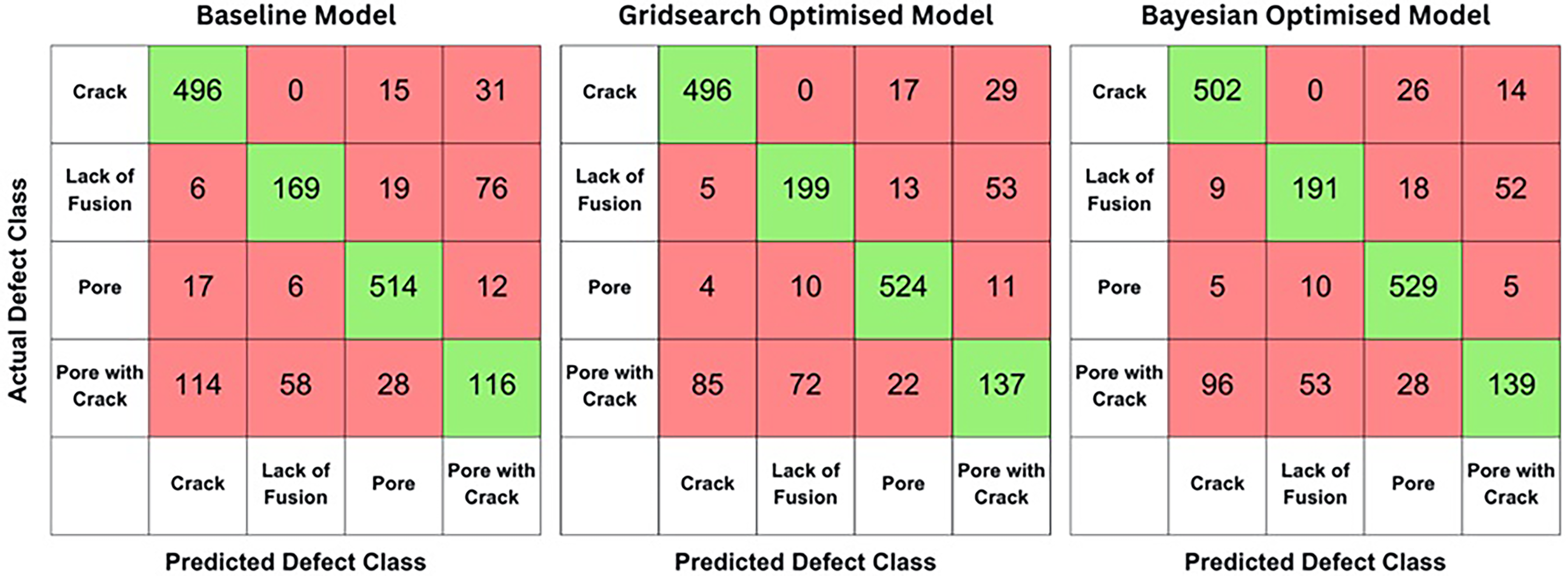
Confusion matrices showing the performance of the baseline, grid-search optimised, and Bayesian optimised models for classifying ‘crack’, ‘pore’, ‘lack of fusion’ and ‘pore with crack’ defects in the synthetic dataset. The validation dataset consists of 1677 instances.

Table 2.

Summary of accuracy for baseline, grid-search optimised, and Bayesian optimised models in correctly classifying defects in the synthetic dataset. The validation dataset consists of 1677 instances.

Defect Type	Baseline Model	Grid-search Optimised Model	Bayesian Optimised Model
Crack	91.5%	91.5%	92.6%
Lack of Fusion	62.6%	73.7%	70.7%
Pore	93.6%	95.4%	96.4%
Pore with Crack	36.7%	43.4%	44.0%
Total	72.2%	80.9%	81.2%

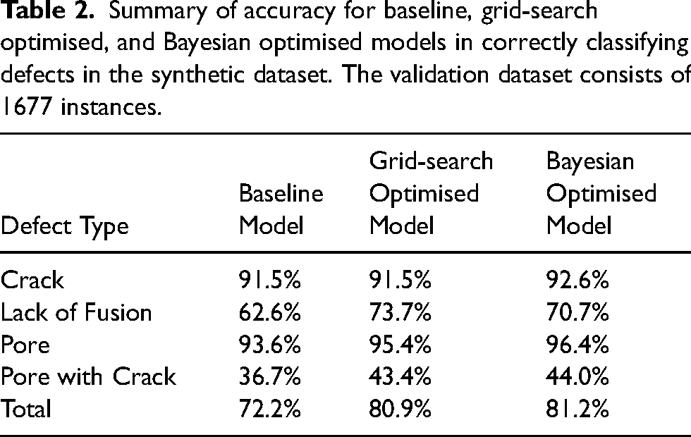
Models trained on the synthetic dataset showed a 10% improvement in ‘pore with crack’ classification for Bayesian optimised models. However, the overall accuracy decreased by roughly 10%, and ‘lack of fusion’ classification accuracy dropped by approximately 15%. This occurs because training on an imbalanced dataset often leads to model bias towards majority classes, resulting in poor generalisation on minority classes.^44,45 By balancing the dataset through augmentation, this bias is reduced, leading to a more evenly distributed classification performance across all classes.

Model evaluation and comparison

It should be noted that other forms of performance metrics, such as sensitivity, precision and recall are also available for model performance evaluation.²⁵ A key consideration is that the synthetic dataset exhibits a different class distribution to the original dataset, with more ‘pore with crack’ defects. For this reason, performance measurement tools must consider both the size of the dataset and the distribution of class labels. By doing so, the models trained on the original dataset and synthetic dataset can by compared, while reflecting these differences. This ensures that the comparisons accurately reflect the models’ abilities to generalise and perform well across varied data distributions and sizes. The Matthews Correlation Coefficient (MCC) is an example of such a performance metric, that was initially used to compare chemical structures,⁵¹ and was then proposed as a standard performance metric for binary and multi-class machine learning applications.^52,53 The MCC has been found to be a reliable metric for evaluating model performance, particularly when comparing different datasets, because it accounts for all four categories of the confusion matrix: true positives, true negatives, false positives, and false negatives.^54–56 Unlike simple accuracy, which only measures the proportion of correctly classified instances, MCC provides a more nuanced assessment by considering the full range of classification outcomes. This makes it especially useful in both binary and multi-class classification problems and when dealing with imbalanced datasets.⁵⁷ The MCC ranges from −1 to +1. An MCC of +1 indicates perfect prediction, 0 suggests no correlation and predictions are no better than random chance, and −1 reflects complete disagreement with entirely incorrect predictions. Table 3 shows the MCC scores for the various models trained.

Table 3.

Matthews correlation coefficient (MCC) scores for ‘crack,’ ‘lack of fusion,’ ‘pore,’ and ‘pore with crack’ defects using baseline, grid-search optimised, and Bayesian optimised models on original and synthetic datasets.

	Original Dataset			Synthetic Dataset
Defect Type	Baseline Model	Grid-search Optimised Model	Bayesian Optimised Model	Baseline Model	Grid-search Optimised Model	Bayesian Optimised Model
Crack	0.862	0.898	0.914	0.767	0.815	0.806
Lack of Fusion	0.828	0.853	0.847	0.618	0.668	0.679
Pore	0.885	0.915	0.930	0.871	0.898	0.880
Pore with Crack	0.139	0.229	0.434	0.315	0.415	0.458

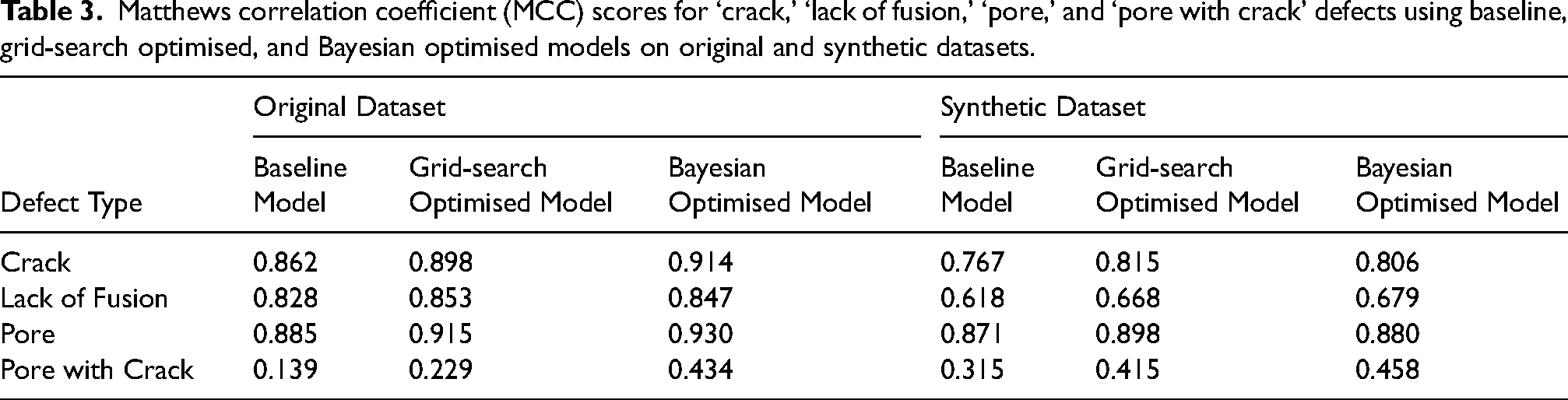
The scores indicate that the models proficiently classify ‘crack’, ‘pore’, and ‘lack of fusion’ defects, whereas ‘pore with crack’ defects are generally less accurately classified. Notably, models optimised using Bayesian optimisation achieved the highest MCC scores overall. While there is a slight improvement in the MCC score for ‘pore with crack’ defects between models trained on the original and synthetic datasets, there is a significant decrease in MCC for the ‘crack’, ‘pore’, and ‘lack of fusion’ defects. This behaviour reflects the trade-off involved in balancing a dataset, as more balanced datasets lead to models that distribute their ability to correctly classify different defects more evenly.

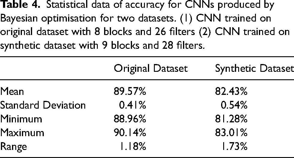
Training neural networks is inherently random due to factors such as shuffled epochs, randomly initialised weights, and biases. Additionally, it is important to note that CNNs require significantly more computational power to train compared to supervised machine learning methods like kNN classification or decision tress. To ensure model robustness, CNNs with architectures optimised through Bayesian optimisation were trained 10 times each with overall accuracy being recorded. Each time a model was trained, the training and validation datasets were randomised completely. Statistical data summarising the average performance are presented in Table 4, showing that the models are robust and perform consistently in terms of accuracy.

Table 4.

Statistical data of accuracy for CNNs produced by Bayesian optimisation for two datasets. (1) CNN trained on original dataset with 8 blocks and 26 filters (2) CNN trained on synthetic dataset with 9 blocks and 28 filters.

	Original Dataset	Synthetic Dataset
Mean	89.57%	82.43%
Standard Deviation	0.41%	0.54%
Minimum	88.96%	81.28%
Maximum	90.14%	83.01%
Range	1.18%	1.73%

Conclusions

This paper has proposed and explored the use of CNNs in the classification of microstructural defects found in additively manufactured nickel-based superalloys. The various CNNs produced have shown good capabilities in classifying the variety of microstructural defects found in additively manufactured nickel-alloys. Classification performance increases as the CNN's architecture becomes more complex, with increased number of layers and filters in the model. CNNs trained on the original dataset and produced by Bayesian optimisation have shown the best performance (approximately 92% accuracy) which is comparable to the accuracy of supervised ML models produced by Aziz et al.,²⁵ and deep learning models produced for other tasks in materials science.^15,16 Despite its success, CNNs have consistently shown poor performance in correctly classifying ‘pore with crack’ defects, due to the lack of data for this defect class and the overlapping features it shares with the ‘pore’ and ‘crack’ classes. To improve the model's classification ability with ‘pore with crack’ defects, data augmentation techniques were used to increase the size of the dataset, creating more ‘pore with crack’ defects for models to train on. While these models, which used synthetic data, showed better performance with ‘pore with crack’ classification, it's classification ability for the ‘crack’, ‘pore’ and ‘lack of fusion’ defects suffered. Supervised ML models produced by Aziz et al.²⁵ also show difficulty with correctly classifying these ‘pore with crack’ defects, suggesting alternative strategies are needed to accurately predict these defects using automated means. To enhance the accuracy of the CNNs developed in this work, expanding the dataset of microstructural defects is recommended, providing the deep learning algorithm with a more diverse and expansive training base. Transfer learning presents another approach to CNN design, which involves repurposing a pretrained CNN for defect classification. This technique can drastically reduce the number of images and computational power needed for training, without much performance drop.¹⁹ Finally, alternative network architectures like Fully Convolutional Networks (FCNs) can directly process images of varying dimensions, which could eliminate resizing errors during preprocessing and improve model robustness and reliability.⁵⁸

Footnotes

Data availability

Supplementary data related to this study are publicly available in a GitHub repository at

Declaration of conflicting interests

The authors declared no potential conflicts of interest with respect to the research, authorship, and/or publication of this article.

Funding

The authors received no financial support for the research, authorship, and/or publication of this article.

References

Mumith

Thomas

Shah

, et al. Additive manufacturing current concepts, future trends. Bone Joint J 2018; 100B: 455–460.

Brischetto

Maggiore

Ferro

. Special issue on “additive manufacturing technologies and applications”. Technologies 2017; 5: 58.

Zhu

Zhou

Wang

, et al. A review of topology optimization for additive manufacturing: status and challenges. Chinese J Aeronaut 2021; 34: 91–110.

Khanzadeh

Chowdhury

Tschopp

, et al. In-situ monitoring of melt pool images for porosity prediction in directed energy deposition processes. IISE Trans 2018; 51: 437–455.

Gorelik

. Additive manufacturing in the context of structural integrity. Int J Fatigue 2017; 94: 168–177.

Brennan

Keist

Palmer

. Defects in metal additive manufacturing processes. J Mater Eng Perform 2021; 30: 4808–4818.

Lorena

Guachi

Stefania

, et al. Automatic microstructural classification with convolutional neural network. In: Botto-Tobar

Barba-Maggi

González-Huerta

Villacrés-Cevallos

Gómez

Uvidia-Fassler

(eds) Information and communication technologies of Ecuador (TICEC). Cham: Springer International Publishing, 2018, pp.170–181.

Lantz

. Machine learning with R. 1st ed. Birmingham: Packt Publishing Limited, 2013.

Alpaydin

. Introduction to machine learning. 3rd ed. Cambridge: MIT Press, 2014.

10.

Snell

Tammas-Williams

Chechik

, et al. Methods for rapid pore classification in metal additive manufacturing. JOM 2020; 72: 101–109.

11.

Scime

Beuth

. Anomaly detection and classification in a laser powder bed additive manufacturing process using a trained computer vision algorithm. Addit Manuf 2018; 19: 114–126.

12.

Nalajam

Ramesh

. Microstructural porosity segmentation using machine learning techniques in wire-based direct energy deposition of AA6061. Micron 2021; 151: 103161.

13.

Ketkar

. Deep learning with python: A hands-on introduction. Berkeley: Apress L.P., 2017.

14.

LeCun

Bengio

Hinton

. Deep learning. Nature 2015; 521: 436–444.

15.

Chowdhury

Kautz

Yener

, et al. Image driven machine learning methods for microstructure recognition. Comput Mater Sci 2016; 123: 176–187.

16.

Durmaz

Müller

Lei

, et al. A deep learning approach for complex microstructure inference. Nat Commun 2021; 12: 6272.

17.

Tan

Zhang

. A deep learning-based method for the design of microstructural materials. Struct Multidisc Optim 2020; 61: 1417–1438.

18.

Beniwal

Dadhich

Alankar

. Deep learning based predictive modeling for structure-property linkages. Materialia 2019; 8: 100435.

19.

Holm

Cohn

Gao

, et al. Overview: computer vision and machine learning for microstructural characterization and analysis. Metall Mater Trans A 2020; 51: 5985–5999.

20.

Jia

Yang

, et al. Quality analysis in metal additive manufacturing with deep learning. J Intell Manuf 2020; 31: 2003–2017.

21.

Després

Cyr

Setoodeh

, et al. Deep learning and design for additive manufacturing: a framework for microlattice architecture. JOM 2020; 72: 2408–2418.

22.

Tian

Guo

Melder

, et al. Deep learning-based data fusion method for in situ porosity detection in Laser-based additive manufacturing. J Manuf Sci Eng 2020; 143: 041011.

23.

Wang

Tan

Tor

, et al. Machine learning in additive manufacturing: state-of-the-art and perspectives. Addit Manuf 2020; 36: 101538.

24.

Qin

, et al. A review of the multi-dimensional application of machine learning to improve the integrated intelligence of laser powder bed fusion. J Mater Process Technol 2023; 318: 118032.

25.

Aziz

Bradshaw

Lim

, et al. Classification of defects in additively manufactured nickel alloys using supervised machine learning. Mater Sci Technol 2023; 39: 2464–2468.

26.

Liu

Selective laser melting of nickel superalloys for aerospace applications: defect analysis and material property optimisation . PhD Thesis, The University of Sheffield, UK, 2021.

27.

Wang

Yuan

. High quality image resizing. Neurocomputing 2014; 131: 348–356.

28.

Srivastava

Hinton

Krizhevsky

, et al. Dropout: a simple way to prevent neural networks from overfitting. J Mach Learn Res 2014; 15: 1929–1958.

29.

Siestma

Dow

RJF

. Creating artificial neural networks that generalize. Neural Netw 1991; 4: 67–79.

30.

LeCun

Boser

Denker

, et al. Handwritten digit recognition with a back-propagation network. In: Touretzky

(ed) Advances in neural information processing systems, Denver, USA. San Mateo: Morgan Kaufmann, 1989, pp.396–404.

31.

Ioffe

Szegedy

. Batch normalization: accelerating deep network training by reducing internal covariate shift. In: Proceedings of the 32nd international conference on machine learning (ICML), Lille, France, 6–11 July 2015. PMLR, pp.448–456.

32.

Nair

Hinton

. Rectified linear units improve restricted Boltzmann machines. In: Proceedings of the 27th international conference on machine learning (ICML), Haifa, Israel, 21–24 June 2010. Omnipress, pp.807–814.

33.

Liu

. Max-pooling convolutional neural networks for vision-based hand gesture recognition. In: Proceedings of the IEEE international conference on neural networks and signal processing, Nanjing, China, 7–11 June 2004. IEEE, pp.597–691.

34.

Bengio

Goodfellow

Courville

. Deep learning. 1st ed. Cambridge, MA: MIT Press, 2017.

35.

Yang

Shami

. On hyperparameter optimization of machine learning algorithms: theory and practice. Neurocomputing 2020; 415: 295–316.

36.

Feurer

Hutter

. Hyperparameter optimization. In: Hutter

Kotthoff

Vanschoren

(eds) Automated machine learning: methods, systems, challenges. Cham: Springer International Publishing, 2019, pp.3–33.

37.

Bartz-Beielstein

Zaefferer

Mersmann

Tuning: methodology. In: Bartz

Bartz-Beielstein

Zaefferer

, et al. (eds) Hyperparameter tuning for machine and deep learning with R: a practical guide. 1st ed. Singapore: Springer, 2023, p.11.

38.

Diaz

Fokoue-Nkoutche

Nannicini

, et al. An effective algorithm for hyperparameter optimization of neural networks. IBM J Res Dev 2017; 61: 1–11.

39.

Antal-Vaida

. Basic hyperparameters tuning methods for classification algorithms. Inform Econ 2021; 25: 64–74.

40.

Ungredda

Branke

. Bayesian Optimisation for constrained problem. ACM Trans Model Comput Simul 2024; 34: 1–26.

41.

Kandasamy

Neiswanger

Schneider

, et al. Neural architecture search with Bayesian optimisation and optimal transport. In: Proceedings of the 32nd international conference on neural information processing systems, Montréal, Canada, 3–8 December 2018. New York: Curran Associates Inc, pp.2020–2029.

42.

Wen

Huang

Guo

. The application of convolutional neural networks (CNNs) to recognize defects in 3D-printed parts. Materials 2021; 14: 2575.

43.

Zhang

Ren

, et al. Deep residual learning for image recognition. In: Proceedings of the IEEE conference on computer vision and pattern recognition (CVPR), Las Vegas, USA, 27–30 June 2016. IEEE, pp.770–778.

44.

Buda

Maki

Mazurowski

. A systematic study of the class imbalance problem in convolutional neural networks. Neural Newt 2018; 106: 249–259.

45.

Garcia

. Learning from imbalanced data. IEEE Trans Knowl Data Eng 2009; 21: 1263–1284.

46.

Skorski

Temperoni

Theobald

. Revisiting weight initialization of deep neural networks. In: Proceedings of the 13th Asian conference on machine learning, Bangkok, Thailand, 17–19 November 2021. Cambridge: PMLR, pp.1192–1207.

47.

Nguyen

Trahay

Domke

, et al. Why globally Re-shuffle? Revisiting data shuffling in large scale deep learning. In: 2022 IEEE international parallel and distributed processing symposium, Lyon, France, 30 May–3 Jun 2022. New York: IEEE, pp.1192–1207.

48.

Taylor

Ojha

Martino

, et al. Sensitivity analysis for deep learning: ranking hyper-parameter influence. In: 2021 IEEE 33rd international conference on tools with artificial intelligence, Washington, USA, 1–3 Nov 2021. New York: IEEE, pp.512–516.

49.

Taylor

Nitschke

. Improving deep learning with generic data augmentation. In: 2018 IEEE symposium series on computational intelligence, Bangalore, India, 18–21 Nov 2018. New York: IEEE, pp.1542–1547.

50.

Shorten

Khoshgoftaar

. A survey on image data augmentation for deep learning. J Big Data 2019; 6: 60.

51.

Matthews

. Comparison of the predicted and observed secondary structure of T4 phage lysozyme. BBA 1975; 405: 442–451.

52.

Baldi

Brunak

Chauvin

, et al. Assessing the accuracy of prediction algorithms for classification: an overview. Bioinformatics 2000; 16: 412–424.

53.

Gorodkin

. Comparing two K-category assignments by a K-category correlation coefficient. Comput Biol Chem 2004; 28: 367–374.

54.

Chicco

Jurman

. The advantages of matthews correlation coefficient (MCC) over F1 score and accuracy in binary classification evaluation. BMC Genomics 2020; 21: 6.

55.

Chicco

Jurman

. The matthews correlation coefficient (MCC) should replace ROC AUC as the standard metric for assessing binary classification. BioData Min 2023; 16: 4.

56.

Chicco

Warrens

Jurman

. The matthews correlation coefficient (MCC) is more informative than Cohen’s kappa and brier score in binary classification assessment. IEEE Access 2021; 9: 78368–78381.

57.

Jurman

Riccadonna

Furlanello

. A comparison of MCC and CEN error measures in multi-class prediction. Plos One 2012; 7: 1–8.

58.

Long

Shelhamer

Darrell

. Fully convolutional networks for semantic segmentation. In: Proceedings of the IEEE conference on computer vision and pattern recognition (CVPR), Boston, USA, 7–12 June 2015. IEEE, pp.3431–3440.

Classification of microstructural defects in selective laser melted inconel 713C alloy using convolutional neural networks

Abstract

Keywords

Introduction

Methodology

Dataset creation and preparation

Data augmentation

Baseline model

Hyperparameter tuning and optimisation

Results and discussion

Original dataset

Synthetic dataset

Model evaluation and comparison

Conclusions

Footnotes

Data availability

Declaration of conflicting interests

Funding

References