Sage Journals: Discover world-class research

Abstract

Human behaviors are complex and composed of changes on multiple time scales. Recent advances in data collection technology contribute to a fast-growing number of studies with rich and intensive longitudinal data, allowing researchers to examine the underlying change processes on the time scale(s) of their choice. Processes unfolding across different time scales can be interrelated in different ways. One way is through reflecting the same underlying construct. For example, attachment styles in couples may lead to a pattern of dyadic coregulation that is reflected both in their physiological synchrony and in their daily affective coherence. Although previous research has examined romantic relationships both from a physiological and an affective perspective, the association between the two has seldom been formally evaluated. In this article, we describe a hierarchical Bayesian vector autoregressive model that enables researchers to examine whether two processes are associated by having coherent patterns. We demonstrate the specification and implementation of this model using data on two different processes between romantic partners: their second-by-second physiological synchrony and daily affect coregulation.

Keywords

dynamic models multiple time scales Bayesian analysis romantic couples intensive longitudinal data

Process-Oriented Thinking in Relationship Research

An essential focus of relationship science is the interdependence of two individuals in a social relationship. A relationship encompasses not only the current state of connectedness between individuals but also their situational feelings and behaviors towards each other, as well as the history of interdependence within this dyad. Therefore, it helps to examine relationships from a process-oriented perspective. A process-oriented thinking highlights the investigation of stability and variability in behaviors for individuals involved in a relationship, and of factors that contribute to such stability and variability (Graber et al., 2011). This is in accordance with Kelley et al.’s (2003) focus on regularities, or “patterns of interdependence” (p. 8), in interpersonal situations. In this framework, regularities include how the individuals influence each other, how information is shared, and how the actions are coordinated and temporally ordered. A process-oriented perspective can also be found in family systems theory, for example, in the concepts of nonlinear causality and homeostasis (Minuchin, 1985). The former notes that the causal chain in relationships is hardly linear (e.g., unsatisfactory performance at work for one partner leads to marital conflicts, which in turn lead to marital dissolution) but circular (e.g., unsatisfactory performance at work on day one leads to marital conflict on the same day, which in turn leads to unsatisfactory performance on day two, and the process goes on). The latter refers to a tendency to maintain established patterns of interaction within relationships.

Dynamic Modeling of Processes

Conceptualizing a relationship as a changing process versus a fixed property has implications for researchers’ analytic approach (and vice versa). Dynamic models provide useful tools to express and uncover the patterns of interdependence in processes. By broad definition, dynamic models are models of change, since they capture how the variables are related over time to themselves and possibly other external factors. The mathematical formulation of dynamic models typically predicts the focal variables (or the changes thereof) at any given time with the previous history of these variables. Doing so explicitly highlights how the modeled association between variables satisfies temporal precedence — a requirement for determining causality (Chambliss & Schutt, 2018). In this way, dynamic models can help researchers describe how individuals influence each other as well as the sequential order of any influence. We take the example of a popular model in relationship science, the actor-partner interdependence model (APIM, Kashy & Kenny, 1999). For each individual in a dyadic relationship, the APIM assesses how their previous behaviors predict their later outcome (“actor” effect), as well as the other individual’s later outcome (“partner” effect; e.g., Cook & Snyder, 2005). When the predictor and the outcome are the same variable(s) merely evaluated at different times (i.e., repeated measures), the APIM is a dynamic model, as the process signified by the outcome variable(s) is now self-propelling (e.g., Cook & Kenny, 2005). In fact, repeated-measures APIM shares ample similarities in expression with the vector autoregressive (VAR) model, a common dynamic model in the time series literature. The VAR model expresses the sequential relations among a set of variables between consecutive observations, assuming that such relations remain the same through the entire process.¹ Figure 1 provides a graphical comparison of a repeated-measures APIM and a bivariate VAR model. Given the parallel between the two model formulations, each dynamic parameter in the VAR model can be conceptualized as a corresponding actor- or partner-effect in APIM. This opens up the possibility of using estimation techniques developed in the time series literature for VAR models to fit an APIM with repeated measures, when the assumption of the VAR model is met. The VAR model and its extensions have been utilized to study dyadic processes such as for mother-infant dyads (e.g., Eason et al., 2020), couples (e.g., Ferrer & Nesselroade, 2003), and peers (e.g., Beltz & Molenaar, 2016). We base our analysis in this article in the VAR model framework and describe the model and the parameters in more detail in Empirical Illustration.

Figure 1.

A graphical display of similarities in an APIM model with repeated measures and a bivariate VAR model of lag one. If we remove the partner labels in APIM, the relations of interest in these two models are mostly identical with intensive longitudinal data.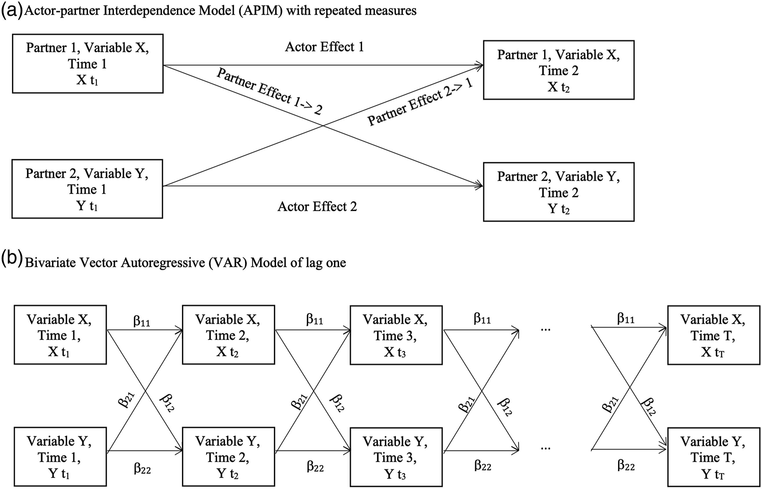

Associations of Processes Across Different Time Scales

Human behaviors are the results of change processes occurring at multiple time scales. They can range from neural processes on the scale of milliseconds to cognitive processes on the scale of seconds or minutes, and to developmental and social processes on the scale of days, months, or even years (Newell, 1990). Typically, actions that are more complex take longer to unfold, as they require more cognitive, emotional, or social resources (Bertenthal, 2007). As an example, a cognitive decision to engage in an interaction with another person takes a few seconds as well as neurons firing in different areas across the brain to perform smaller tasks such as facial recognition, emotion perception, and situational evaluation. A social interaction with this person takes minutes or hours and requires rapid decision-making based on the information being communicated. A relationship developed with this person takes weeks or months and involves many incidents of social interactions. All the examples given above can be used to study relationships, but each of these processes evolves on a different time scale from the others.

Associations of processes across different time scales have been described in theories and empirical studies in at least three ways: 1. as trait-and-state relationships through self-organization, 2. as cross-level adaptations via bidirectional influences, and 3. as patterns reflecting the same underlying construct. In this article, we illustrate a method that helps to investigate the third kind, but we would like to briefly describe and discuss the former two as they are equally interesting. For ease of clarification, we will focus on explaining the association between two processes, but these categories can be generalized to include more than two processes as well.

The first type of association across time scales is through self-organization. This is when one of the processes is a macro-level (or “trait-level”) developmental process and the other is a micro-level (or “state-level'') change process. Self-organization refers to when patterns in the macro-level process arise from seemingly disordered interactions in the micro-level process (Kelso, 1995). In this situation, the macro-level governs the micro-level process, or alternatively, the micro-level process is an expression of the macro-level process. One example of such two processes is an emotional experience in real-time (micro) and the development of personality (macro; Lewis & Ferrari, 2001). The increased likelihood of certain emotions (and decreased likelihood of others) over time describes the development of certain personality traits. The emotional experience at the micro-scale both contributes to, and is limited by, the personality at the macro-scale. This is similar to the concepts of “warp and woof of the developmental fabric'' (Nesselroade, 1991, p. 213), or intraindividual change and intraindividual variability.

The second type of association across time scales is through bidirectional influences (Gottlieb, 1991). This type of association would manifest in a (often negative) feedback loop, with one process stimulating the other, and the other dampening the original process in return. An example of such an association is that between physiological reactions and behavioral responses in emotion. The common understanding of emotional processing pathways is that sensory input from a stimulus travels down two paths: a “fast path” that is an instinctive response and a “slow path” that involves cognitive processing (LeDoux, 2003). A stimulus imposes a demand and elicits an immediate physiological response (“fast path”) such as racing heartbeats and sweating. Information on such physiological changes is then acknowledged by the “slow path” of executive functioning (and thus requires more cognitive resources). The behavioral response as an outcome of the “slow path” then regulates the previously elicited physiological responses (Torrisi et al., 2013).

The third type of association across time scales, and our focus in this article, is through latent constructs. Two processes associated in this way define (or are manifestations of) the same underlying construct. This taps into the measurement of underlying psychological constructs, as they are created as an assembly of observed patterns or profiles to help understand human behaviors. Here we use attachment as an example of the underlying construct. Adult a m m8ittachment can be conceptualized as a trait-level characteristic that stays relatively stable during the observed period of expressions (Sbarra & Hazan, 2008; Shaver & Mikulincer, 2002). Individuals with high attachment anxiety would develop a maladaptive working model of their relationships with others that hinders their ability to successfully manage distress in their everyday lives (Mikulincer & Shaver, 2019). In physiological signals, this maladaptive working model manifests in heightened stress response and hypervigilance (Feeney & Kirkpatrick, 1996; Roisman, 2007). In behaviors, it manifests in a higher occurrence of proximity seeking (Shaver & Mikulincer, 2002), and in emotion regulation, it manifests in prolonged depressive mood (Zheng et al., 2020). If we can observe more than one manifestation for the same individual, it is reasonable to expect this individual to show some consistency in patterns across different processes, based on their attachment styles.

Modeling Association Between Patterns in Different Time Scales

Advances in data collection technology contribute to a fast-growing number of studies utilizing methods such as EMA and/or noninvasive monitoring, and to the richness of data researchers can collect. Therefore, it is now possible to examine processes on different levels of analysis in the same study, and to study the relationship between processes on different time scales.

In this article, we describe a modeling approach for assessing associations across time scales with the same underlying construct (the third type) and provide an illustration based on a multilevel VAR model. Here, we operationalize “association” across time scales as the relation between each dyad’s dynamic parameters in the two time scales. Mathematically, dynamic parameters determine how a process unfolds in time, and thus, are descriptive of the patterns that relationship research concerns. By adopting a multilevel model, we assume that there is a population-average pattern on each time scale and individual dyads show deviations from the average. When the association by construct is present between time scales, the deviations would show systematic trends. Using the previous example on attachment anxiety, it would be reasonable to expect an individual who exhibits higher-than-average stress responses to also exhibit more-than-average proximity seeking when facing a stressor.

With the combination of intensive longitudinal data, multivariate dynamic models, and random effects, the derivation of sample-level likelihood to perform statistical inference on the parameters is no longer trivial. In this case, it is easier for researchers on the users' end to fit this model in the Bayesian framework. Bayesian tools allow us to include models for the two processes with correlated random effects in an integrated overall model, thus assessing all relations and associations of interest simultaneously in one step. Implementing this one-step approach has advantages over previous work using two steps (e.g., Ferrer & Helm, 2013). In two-step approaches, parameters are estimated within each individual unit of analysis (e.g., person, dyad, family), and then, the association between processes is evaluated using estimated parameters as trait-level data. Using a one-step approach, we are able to preserve the uncertainty around the individual estimates as it is factored into the overall likelihood, thus avoiding the potential error in inference due to reduced variability from treating estimates as observed data. Our goal in the article is to demonstrate the feasibility of assessing such association across time scales using easy extensions to common models and readily available analytic tools. We hope this article will serve as an example of how researchers can formally evaluate the extent of association between dynamic processes of relationship.

Empirical Illustration: Couples’ Physiological and Affective Interactions

Attachment styles can be defined as innate patterns of interactive behaviors and regulatory strategies that define the social interactions between any certain pair (Bowlby, 1982). By this definition, attachment styles of romantic partners shape the working model of the relationship and their interactions. Thus, such a working model should lead to coherent patterns in different interactive processes within the same couple.

In this article, we examined two processes: daily affect and physiological signals. Both of these are regulatory processes that, when studied within one individual, have self-regulatory properties that maintain them in a controllable range (Kuppens et al., 2010; Porges, 2007). In this article, we define self-regulation rather broadly as a goal-directed behavior of change that takes the previous history as input. In different contexts, self-regulation is evidenced by the increase, decrease, or maintenance of certain observable quantities with respect to a goal (e.g., positive vs. negative affect, Kuppens et al., 2010). When these two processes are examined in interpersonal situations, a second driving force, coregulation, comes into effect in addition to self-regulation. Coregulation within dyads refers to how either individual is up- or down-regulated by their partner, or in other words, influences between dyad members (Sbarra & Hazan, 2008).

Romantic partners' affective experiences were shown to covary in their daily lives, after the influence from shared activities was accounted for (Butner et al., 2007). When an emotional experience happens in a social situation or a relationship, it becomes an interpersonal emotion, as components of such emotional experience (e.g., behaviors, physiology) are transmitted and perceived by others (including the partner), and vice versa (Butler, 2011). How emotional signals are displayed and perceived, then, is governed by both partners' temperament and personality, as well as their romantic attachment. For example, an individual who is more emotionally attuned may identify their partner’s emotional states more accurately, and their history in this relationship would determine their behavioral responses to their partner. Hence, we expect the couple’s everyday affective patterns to reflect their established way of interaction, and in turn, the inner working model of their relationship.

At the same time, interaction and coregulation in romantic relationships have also been investigated with the interdependence of physiological signals (Sbarra & Hazan, 2008). Among the physiological signals, those from the autonomic nervous system (such as cardiac activity and respiration) reflect the body’s response to situational demands and are frequently utilized in studies of interpersonal situations. Physiological interdependence, often referred to as physiological synchrony, has been linked to various psychosocial constructs and is considered informative of social interactions (see Palumbo et al., 2017, for a systematic review of research on physiological synchrony in different populations). Therefore, we expect a couple’s physiological pattern, when they are attending to their partners, to also reflect the inner working model of their relationship.

Previous studies have explored either process on its own and suggested that the two processes might be related. Researchers have examined the dynamic interplay between partners in the daily process of relationship-specific affect, with analyses based on either a coupled damped oscillator model (Boker & Nesselroade, 2002), a linear second order differential equation model (Steele & Ferrer, 2011), or a linear first order differential equation model (Steele et al., 2014). In addition, Ferrer and Steele (2014) explored a few nonlinear variations of the first-order model, focusing on different possible forms of interactions. Most of the models explored had both a self-regulation (within-individual temporal influence) and a coregulation (between-partner temporal influence) component, thus making them plausible for the phenomenon. The same models were also applied to dyadic intensive time-series data on heart rate and respiration collected in a laboratory setting (Ferrer & Helm, 2013; Helm et al., 2012). In all these studies, the models of choice were fit to each dyad in the sample individually, and the results supported heterogeneity within the sample in model parameters. Steele et al. (2014) also investigated the association between interaction patterns (represented by individual dynamic parameter estimates) and trait-level dyadic characteristics, such as attachment and relationship satisfaction. Results showed moderate links between several facets of interaction patterns and these trait-level characteristics. In addition, Ferrer and Helm (2013) found correlations between the females' coregulation parameters from their physiological process and from their daily affective process in their two-step analysis.

Based on these premises, we are interested in examining whether dynamic patterns of interactions for the same romantic partners are consistent across different measurements and across time scales when formally assessed in a model. In this article, we considered two processes: a) the couples' second-by-second cardiac arousal during a laboratory task and b) their day-to-day relationship-specific affective experience. The two-step individual model-fitting analytic approach in Ferrer and Helm (2013) provides a crude approximation to the estimation problem of association across time scales. In the one-step analytic approach utilized in this article, both processes were modeled with the association between these processes assessed simultaneously. We also explore, in the same model, whether the association can be predicted by couples’ trait-level characteristics.

Method

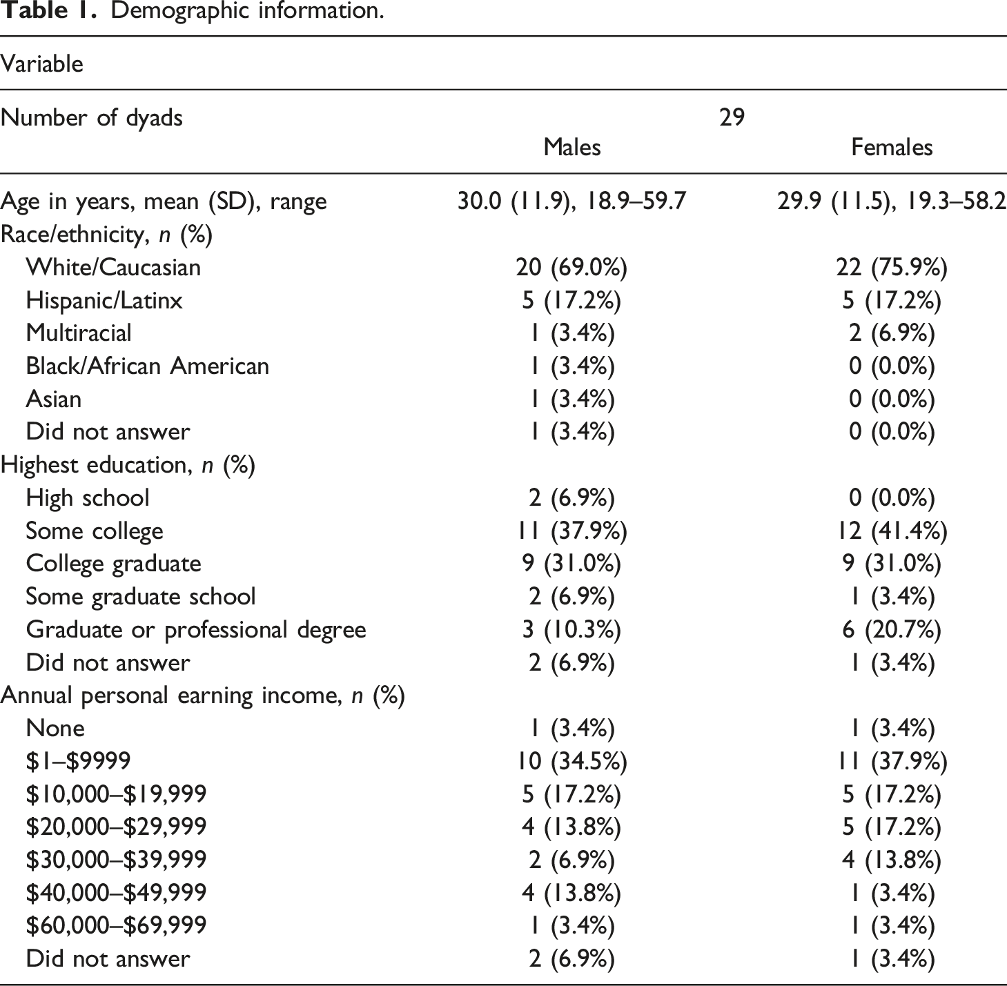
Participants

This illustration used previously published dyadic data on romantic couples from the Dynamics of Dyadic Interactions Project (DDIP, see e.g., Ferrer & Widaman, 2008). Three hundred and 36 cisgender heterosexual couples were recruited for this large project through advertisements online as well as in local newspapers. Out of these 336 dyads, 32 completed the laboratory tasks for physiological measures, and 304 participated in daily reporting of affect for up to 90 consecutive days since their enrollment in the project. In our study, we included a total of 29 dyads whose data were collected for both the laboratory and the daily diary sections of the study for both partners. Demographic information of these 29 dyads is reported in Table 1.

Table 1.

Demographic information.

Variable
Number of dyads	29
Number of dyads	Males	Females
Age in years, mean (SD), range	30.0 (11.9), 18.9–59.7	29.9 (11.5), 19.3–58.2
Race/ethnicity, n (%)
White/Caucasian	20 (69.0%)	22 (75.9%)
Hispanic/Latinx	5 (17.2%)	5 (17.2%)
Multiracial	1 (3.4%)	2 (6.9%)
Black/African American	1 (3.4%)	0 (0.0%)
Asian	1 (3.4%)	0 (0.0%)
Did not answer	1 (3.4%)	0 (0.0%)
Highest education, n (%)
High school	2 (6.9%)	0 (0.0%)
Some college	11 (37.9%)	12 (41.4%)
College graduate	9 (31.0%)	9 (31.0%)
Some graduate school	2 (6.9%)	1 (3.4%)
Graduate or professional degree	3 (10.3%)	6 (20.7%)
Did not answer	2 (6.9%)	1 (3.4%)
Annual personal earning income, n (%)
None	1 (3.4%)	1 (3.4%)
$1–$9999	10 (34.5%)	11 (37.9%)
$10,000–$19,999	5 (17.2%)	5 (17.2%)
$20,000–$29,999	4 (13.8%)	5 (17.2%)
$30,000–$39,999	2 (6.9%)	4 (13.8%)
$40,000–$49,999	4 (13.8%)	1 (3.4%)
$60,000–$69,999	1 (3.4%)	1 (3.4%)
Did not answer	2 (6.9%)	1 (3.4%)

Procedure

Laboratory Tasks

A subset of participating couples were asked to complete a series of laboratory tasks: baseline, gazing, and imitation, with their physiological signals monitored the entire time. Participants in each dyad were instructed to sit in armchairs placed three feet apart from each other and to avoid physical contact during all tasks. In the baseline task, they were asked to relax for 5 minutes, refraining from bodily movements, facial gestures, and vocal noises. In the gazing task, they were asked to maintain eye contact with their partner for 3 minutes. Finally, in the imitation task, they were asked to “mirror” their partner’s physiological responses. They were told that this final task was abstract and that direct knowledge of how to perform it was lacking.

Daily Questionnaires

Participants were asked to complete paper-pencil questionnaires daily after initial enrollment in the project for up to 90 days. Each partner in a couple completed their own set of questionnaires separately from the other. The daily questionnaires contained various items on general and relationship-specific affect, as well as hours spent with the partner and number of times communicated with the partner, and a free response space to describe any major event during the day. The average number of daily questionnaires completed by the 29 dyads in our sample was 78.6 (with a minimum of 24.0 and a maximum of 96.0).

Measures

Cardiac Arousal

In this study, we focus on the physiological synchrony patterns in cardiac activities during the imitation task. Cardiac arousal was measured using electrocardiogram (ECG) with interbeat intervals (IBIs) at 1000 samples per second for the laboratory tasks. IBI is the time elapsed between consecutive heartbeats, and a higher value of IBI indicates less cardiac arousal. The software MindWare (Mindware Technologies LTD., Westerville, OH) was used to identify heartbeats and derive IBIs. The IBI output for each participant was then reconfigured to an equidistant time series to ensure that the time indices of measurements matched between the two partners (Appendix A in Ferrer and Helm (2013) contains a detailed description of the transformation). Finally, the time series were reduced in frequency by keeping only the first of every 20 observations, so that the time indices were spaced at one second, resulting in an average of 177.8 seconds of IBIs per dyad and a standard deviation of 0.95 seconds across dyads (min. = 174, max. = 179). Within the time series for each individual, missing data occurred for an average of 1.0% for males and 1.1% for females (with a maximum of 3.3% for both). If the missing data were at the beginning or the end of a time series, then they were deleted, with the time index for the first available observation relabeled as the first time index. If they were between observed data (with a maximum of 1.7% for males and 2.8% for females, and an average of 0.1% for both), then they were interpolated using the mean of this individual.

Relationship-Specific Affect

The set of items for relationship-specific affect was developed by the DDIP team. It encompassed 18 items that aimed to describe the emotional experience related to the romantic relationship. Participants were asked to “Indicate to what extent you have felt this way about your relationship today” using a 5-point Likert-type scale, from 1 (“very slightly or not at all”) to 5 (“extremely”) with a midpoint of 3 being “moderately”. Half of the 18 items described positive experiences: “emotionally intimate”, “physically intimate”, “trust”, “committed”, “free”, “loved”, “loving”, “happy”, and “socially supported”. The other half described negative experiences: “sad”, “blue”, “trapped”, “argumentative”, “discouraged”, “doubtful”, “lonely”, “angry”, and “deceived”. Internal consistency and reliability of these measures of systematic change across days were assessed in previous studies (Ferrer & Widaman, 2008; Steele et al., 2014). We computed the average of positive and negative affect items separately. Then a ratio of positive over all affect was calculated as an integrated measure of positive and negative affect, under the theory of a balanced state of mind (Schwartz, 1997). The same missing data handling strategy as in IBIs was used for the affect scores. On average, data were missing 6.0% of the time for males and 6.2% of the time for females (with a maximum of 34.4% and 35.5% for males and females respectively). After truncating the missing data at the beginning and the end of the time series, the missingness was reduced to an average of 4.7% for males (max. = 33.3%) and 5.0% for females (max. = 23.3%).

Dyad-Level Traits

Participants completed a first-visit questionnaire that contained demographic information as well as information related to their relationship. In this study, we are concerned mainly with traits specific to their attachment and relationship quality. Scores on these traits were averaged between two partners to obtain dyad-level measurements. Attachment-related avoidance and anxiety were measured for each partner using the Experiences in Close Relationship Scales (Brennan et al., 1998). Relationship quality was measured using a previously validated questionnaire (Fletcher et al., 2000) that contained six 7-point Likert-type scale items, each corresponding to a different underlying dimension of relationship quality such as satisfaction, commitment, and intimacy. Mean composite scores were created from these six items for an overall measure of relationship quality.

Model and Analysis

The model we employed consisted of two parts, the model for second-by-second IBIs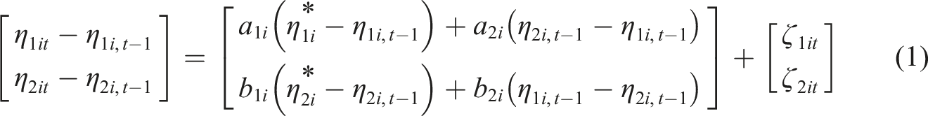

\begin{array}{c} [\begin{array}{c} η_{1 i t} - η_{1 i, t - 1} \\ η_{2 i t} - η_{2 i, t - 1} \end{array}] = [\begin{array}{c} a_{1 i} (η_{1 i}^{*} - η_{1 i, t - 1}) + a_{2 i} (η_{2 i, t - 1} - η_{1 i, t - 1}) \\ b_{1 i} (η_{2 i}^{*} - η_{2 i, t - 1}) + b_{2 i} (η_{1 i, t - 1} - η_{2 i, t - 1}) \end{array}] + [\begin{array}{c} ζ_{1 i t} \\ ζ_{2 i t} \end{array}] \end{array}

(1)

\begin{array}{c} [\begin{array}{c} ζ_{1 i t} \\ ζ_{2 i t} \end{array}] \sim N ([\begin{array}{c} 0 \\ 0 \end{array}], [\begin{array}{c} σ_{ζ 1}^{2} & σ_{ζ 12} \\ σ_{ζ 12} & σ_{ζ 2}^{2} \end{array}]), \end{array}

(2)

and the model for daily relationship-specific affect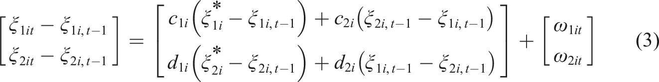

\begin{array}{c} [\begin{array}{c} ξ_{1 i t} - ξ_{1 i, t - 1} \\ ξ_{2 i t} - ξ_{2 i, t - 1} \end{array}] = [\begin{array}{c} c_{1 i} (ξ_{1 i}^{*} - ξ_{1 i, t - 1}) + c_{2 i} (ξ_{2 i, t - 1} - ξ_{1 i, t - 1}) \\ d_{1 i} (ξ_{2 i}^{*} - ξ_{2 i, t - 1}) + d_{2 i} (ξ_{1 i, t - 1} - ξ_{2 i, t - 1}) \end{array}] + [\begin{array}{c} ω_{1 i t} \\ ω_{2 i t} \end{array}] \end{array}

(3)

\begin{array}{c} [\begin{array}{c} ω_{1 i t} \\ ω_{2 i t} \end{array}] \sim N ([\begin{array}{c} 0 \\ 0 \end{array}], [\begin{array}{c} σ_{ω 1}^{2} & σ_{ω 12} \\ σ_{ω 12} & σ_{ω 2}^{2} \end{array}]) \end{array}

(4)

These two models are essentially VAR models with a lag of one (VAR(1) models) reparametrized to resemble the differential equation model by Felmlee and Greenberg (1999), which was used in prior analyses of the two processes separately (Ferrer & Helm, 2013; Steele et al., 2014)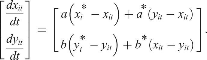

\begin{array}{c} [\begin{array}{c} \frac{d x_{i t}}{d t} \\ \frac{d y_{i t}}{d t} \end{array}] = [\begin{array}{c} a (x_{i}^{*} - x_{i t}) + a^{*} (y_{i t} - x_{i t}) \\ b (y_{i}^{*} - y_{i t}) + b^{*} (x_{i t} - y_{i t}) \end{array}] . \end{array}

In fact, through exact discrete models (see e.g., Oud & Jansen, 2000), there is a one-to-one correspondence between linear first order differential equation models and VAR(1) models. Since the time elapsed between measurements in both processes can be conceptualized as equal (second-by-second and daily), we decided to utilize a VAR(1) model instead of its continuous-time counterpart to ease the computational cost during model fitting.

As our sample consisted only of heterosexual couples, we labeled the variables and parameters associated with the male partners with a subscript 1 and those with female partners with a subscript 2. Therefore, in equation (1), $η_{1 i t}$ represents the IBIs of the male partner in dyad i at time t, and in the emotional process model, equation (3), $ξ_{i t}$ represents the relationship-specific affect, again for the male partner in dyad i at time t (vice versa, $η_{2 i t}$ and $ξ_{2 i t}$ for the female partner in dyad i). The processes in equations (1)–(4) are governed by the following three groups of parameters:

Self-Regulation Parameters

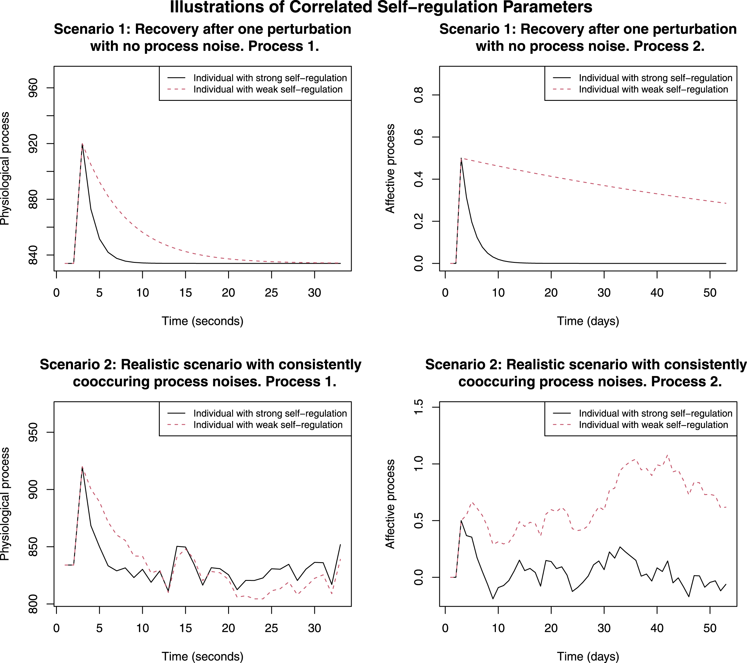
For an arbitrary dyad i, $a_{1 i}$ and $c_{1 i}$ govern how much the change in the male partner between two measurement occasions is determined by the distance between his former measurement and his setpoint $η_{1 i}^{*}$ and $ξ_{1 i}^{*}$ (here we define the setpoint as a state with longer-term stability without perturbation or influence from the other partner)², for the physiological process and the affective process respectively. In the physiological process, the setpoint was set to everyone’s average IBI during the baseline task. In the daily affective process, it was set to their mean score across all days. $b_{1 i}$ and $d_{1 i}$ govern the same change tendency in females for the psychological and emotional processes. Since these parameters characterize how individuals change with respect to themselves, in this article we refer to these parameters as self-regulation parameters. As demonstrated in Figure 2 (left panel), a higher (positive) value for the self-regulation parameter in this model indicates that the individual recovers more quickly back to their setpoint after perturbations compared to the individuals with lower values.

Figure 2.

Simulated processes of partner 1 from equations (1) and (2) with different values of self-regulation (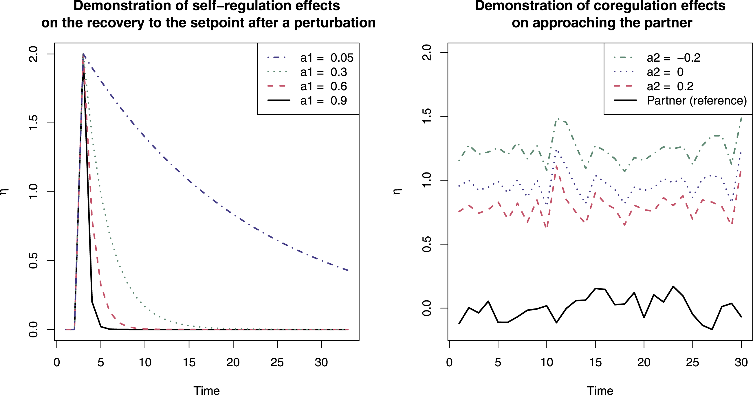 $a_{1}$ , left panel) and coregulation parameters ( $a_{2}$ , right panel). For the plot of coregulation parameters, partner 2’s trajectory is plotted as a reference (black solid line) and remains the same when generating data based on different coregulation parameter values to demonstrate its influence on the focal person’s trajectory. For the right panel, $a_{1} = 0.9$ , $b_{1}$ (the partner’s self-regulation parameter) = 0.5, $σ_{ζ 1}^{2} = σ_{ζ 2}^{2}$ (the variance of perturbation magnitudes) = 0.01. Setpoint $η_{1 i}^{*}$ is set to zero in the left panel and one in the right panel, and $η_{2 i}^{*}$ in the right panel is zero. Other parameters in equations (1) and (2) not specified above are fixed at zero.

Coregulation Parameters

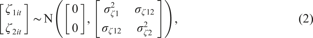
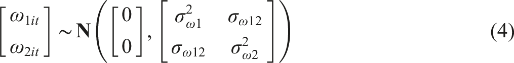
Between-partner influences are governed by the coregulation parameters, namely, $a_{2 i}$ (female to male, physiological process), $b_{2 i}$ (male to female, physiological process), $c_{2 i}$ (female to male, emotional process), $d_{2 i}$ (male to female, emotional process). These parameters determine the influences of the distance between the two partner’s previous states on the processes, or in other words, how much one partner adapts given the previous status of the other partner. The right panel Figure 2 shows two hypothetical scenarios of coregulation parameters, a positive value leads an individual closer to their partner (red dashed line), whereas a negative value repels this individual away from their partner (green dot-and-dash line) from their usual trajectory without the influence of a partner (blue dotted line).

Process Noise Parameters

The last terms of Equations (1) and (3), $ζ$ ’s and $ω$ ’s, represent the white noises in the two processes. Those are random fluctuations in the processes that are not determined by the focal process variables, or any other observed information. They are assumed to take on a multivariate normal distribution with a full covariance matrix for each process. The covariance matrix quantifies the scale of these fluctuations.

Since heterogeneity in the dynamic parameters was suggested in previous explorations, the four key regulatory parameters for either process were modeled with mixed effects. Since we were interested in exploring interaction patterns as particular to each dyad, we included other trait-level predictors in the mixed effect equations, resulting in

θ_{i} = β_{θ 0} + β_{θ 1} a n x_{i} + β_{θ 2} a v o_{i} + β_{θ 3} r e l_{i} + γ_{θ i}

(5)

θ \in {{a_{1}, a}_{2}, b_{1}, b_{2}, c_{1}, c_{2}, d_{1}, d_{2}} .

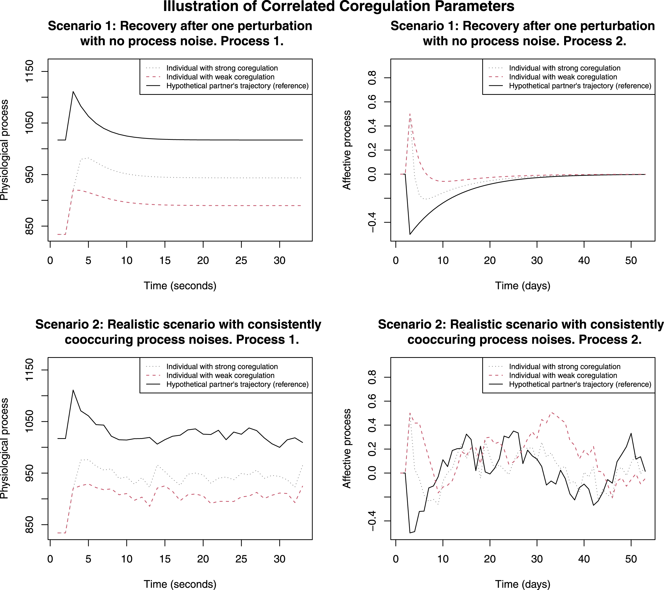
As we adopted models of identical formulation for the mixed effects, here we use $θ$ to avoid repetition of equations. In the above equation, $θ_{i}$ represents any of the mixed-effect parameters, whereas $a n x_{i}$ and $a v o_{i}$ are the attachment-related anxiety and avoidance (Brennan et al., 1998) for dyad i collected at the beginning of the study, and $r e l_{i}$ is the relationship quality for this dyad collected after the participants finished the daily self-reports part of the study.

The random effects $(γ_{θ i})$ of the dynamic parameters were assumed to follow multivariate normal distributions with mean 0. To evaluate whether there were associations between the two processes, we allowed for correlations between the corresponding parameters (e.g., $a_{1}$ and $c_{1}$ which are both self-regulatory parameters for males: $a_{1}$ for the physiological process and $c_{1}$ for the emotional process). Figures 3 and 4 provide simulated illustrations of how correlated parameters (self-regulation and coregulation, respectively) manifest across the two processes in different time scales.

[\begin{array}{c} γ_{a 1 i} \\ γ_{c 1 i} \end{array}] \sim N (0, [\begin{array}{c} σ_{γ a 1}^{2} & σ_{a 1 c 1} \\ σ_{a 1 c 1} & σ_{γ c 1}^{2} \end{array}]); [\begin{array}{c} γ_{b 1 i} \\ γ_{d 1 i} \end{array}] \sim N (0, [\begin{array}{c} σ_{γ b 1}^{2} & σ_{b 1 d 1} \\ σ_{b 1 d 1} & σ_{γ d 1}^{2} \end{array}])

(6)

[\begin{array}{c} γ_{a 2 i} \\ γ_{c 2 i} \end{array}] \sim N (0, [\begin{array}{c} σ_{γ a 2}^{2} & σ_{a 2 c 2} \\ σ_{a 2 c 2} & σ_{γ c 2}^{2} \end{array}]); [\begin{array}{c} γ_{b 2 i} \\ γ_{d 2 i} \end{array}] \sim N (0, [\begin{array}{c} σ_{γ b 2}^{2} & σ_{b 2 d 2} \\ σ_{b 2 d 2} & σ_{γ d 2}^{2} \end{array}])

(7)

Figure 3.

A simulated demonstration of how correlated self-regulation parameters (e.g., $a_{1}$ and $c_{1}$ , the self-regulation parameters for males in the two processes) manifest in the trajectories across different time scales. Data were generated according to Equations (1)–(4) for hypothetical individuals with parameter values resembling the values in our empirical example (except for the correlation parameter, as we did not detect a meaningful correlation). All other parameters except for $a_{1}$ and $c_{1}$ are identical for the two individuals ( $a_{2} = c_{2} = b_{2} = d_{2} = 0$ ). For $a_{1}$ and $c_{1}$ , we drew 100 samples from a multinormal distribution with mean (0.3, 0.1) and covariance matrix $[\begin{array}{c} 0.01 & 0.009 \\ 0.009 & 0.01 \end{array}]$ and selected the maximum and minimum in the sample to maximize the visual difference for demonstrative purposes. An identical time series of random process noises are added to the two individuals' trajectories in either plot in the bottom row. When the two processes are positively correlated, individuals who are stronger/weaker in self-regulation in one time scale are also stronger/weaker in the other, demonstrated by how fast the process returns to its setpoint (physio: 834, affect: 0) after perturbed.

Figure 4.

A simulated demonstration of how correlated coregulation, or in other words, synchronizing tendency, parameters (e.g., $a_{2}$ and $c_{2}$ , the female-to-male effects/coregulation parameters in the two processes) manifest in the trajectories across different time scales. Again, data were generated according to Equations (1)–(4) for hypothetical individuals. All other parameters except for $a_{2}$ and $c_{2}$ are set to resemble the values in our empirical example and are identical for the two individuals ( $a_{1} = b_{1} = 0.3, c_{1} = d_{1} = 0.1$ ). For $a_{2}$ and $c_{2}$ , we drew 100 samples from a multinormal distribution with mean (0.1, 0.1) and covariance matrix $[\begin{array}{c} 0.01 & 0.009 \\ 0.009 & 0.01 \end{array}]$ and selected the maximum and minimum in the sample to maximum the visual difference for demonstrative purposes. For illustrative purposes, the partner’s process is also held identical for the two individuals. An identical series of random system noises is added to the two individuals’ trajectories for either plot in the bottom row. When the two processes are positively correlated, individuals with stronger/weaker tendency to reduce the distance to their partner would show consistent tendency in both processes.

Equations (1) through (7) were combined into a full hierarchical model and fit using Stan (Carpenter et al., 2017) interfaced from R (R Core Team, 2018) through the package rstan (Stan Development Team, 2020). Affect data were standardized within-person before model fitting. When fitting the model, we utilized four chains for the Markov chain Monte Carlo sampling. Each chain contains 2000 iterations of warmup and 10000 iterations of sampling.³ Examination of the $\hat{R}$ statistics (Gelman et al., 1992) did not indicate any problem with convergence. However, the tail or bulk effective sample size (ESS) for a few parameters fell below the recommended number of 100 per chain (Stan Development Team, 2020; Vehtari et al., 2020). We would like to note here that a low ESS indicates low sample efficiency in the bulk or tail area of the posterior sample for Bayesian inference, thus impacting the reliability of the central tendency measures (such as mean, median, and mode) or the credible intervals. For illustration purposes, we go ahead and interpret the results, but in practice, caution should be exercised when ESS is lower than recommended.

Results

In the result examination, we concluded that an effect was credibly different from zero if the 95% credible interval for that parameter did not include zero. For variance parameters that are by nature non-negative, we took 0.001 as an arbitrarily small value. If the credible interval for a variance parameter had a lower bound greater than 0.001, then we would conclude that the variance was nonignorable. Table 2 contains a summary of results for fixed effect parameters and Table 3 for random effect parameters.

Table 2.

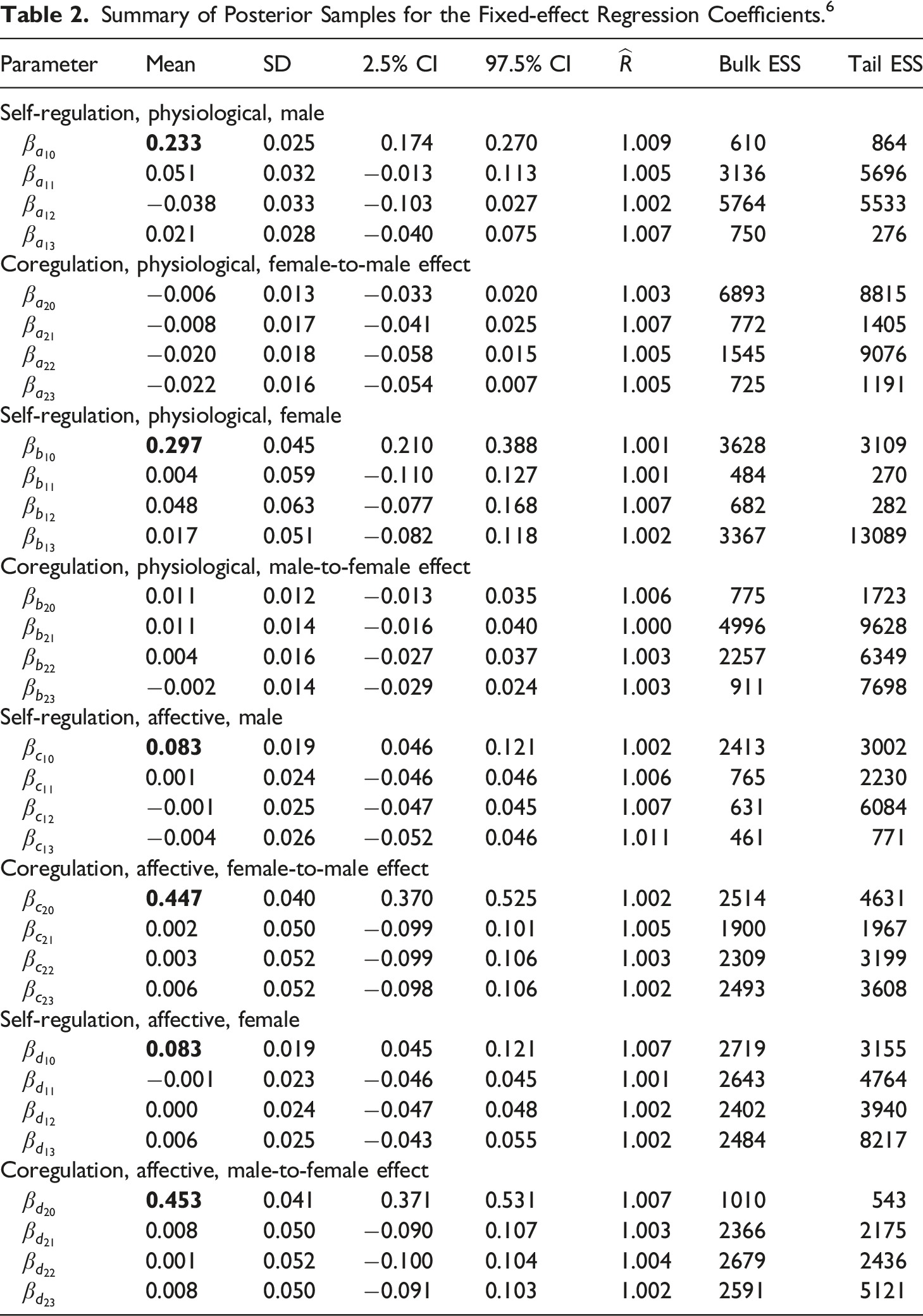
Summary of Posterior Samples for the Fixed-effect Regression Coefficients.⁶

Parameter	Mean	SD	2.5% CI	97.5% CI	$\hat{R}$	Bulk ESS	Tail ESS
Self-regulation, physiological, male
$β_{a_{10}}$	0.233	0.025	0.174	0.270	1.009	610	864
$β_{a_{11}}$	0.051	0.032	−0.013	0.113	1.005	3136	5696
$β_{a_{12}}$	−0.038	0.033	−0.103	0.027	1.002	5764	5533
$β_{a_{13}}$	0.021	0.028	−0.040	0.075	1.007	750	276
Coregulation, physiological, female-to-male effect
$β_{a_{20}}$	−0.006	0.013	−0.033	0.020	1.003	6893	8815
$β_{a_{21}}$	−0.008	0.017	−0.041	0.025	1.007	772	1405
$β_{a_{22}}$	−0.020	0.018	−0.058	0.015	1.005	1545	9076
$β_{a_{23}}$	−0.022	0.016	−0.054	0.007	1.005	725	1191
Self-regulation, physiological, female
$β_{b_{10}}$	0.297	0.045	0.210	0.388	1.001	3628	3109
$β_{b_{11}}$	0.004	0.059	−0.110	0.127	1.001	484	270
$β_{b_{12}}$	0.048	0.063	−0.077	0.168	1.007	682	282
$β_{b_{13}}$	0.017	0.051	−0.082	0.118	1.002	3367	13089
Coregulation, physiological, male-to-female effect
$β_{b_{20}}$	0.011	0.012	−0.013	0.035	1.006	775	1723
$β_{b_{21}}$	0.011	0.014	−0.016	0.040	1.000	4996	9628
$β_{b_{22}}$	0.004	0.016	−0.027	0.037	1.003	2257	6349
$β_{b_{23}}$	−0.002	0.014	−0.029	0.024	1.003	911	7698
Self-regulation, affective, male
$β_{c_{10}}$	0.083	0.019	0.046	0.121	1.002	2413	3002
$β_{c_{11}}$	0.001	0.024	−0.046	0.046	1.006	765	2230
$β_{c_{12}}$	−0.001	0.025	−0.047	0.045	1.007	631	6084
$β_{c_{13}}$	−0.004	0.026	−0.052	0.046	1.011	461	771
Coregulation, affective, female-to-male effect
$β_{c_{20}}$	0.447	0.040	0.370	0.525	1.002	2514	4631
$β_{c_{21}}$	0.002	0.050	−0.099	0.101	1.005	1900	1967
$β_{c_{22}}$	0.003	0.052	−0.099	0.106	1.003	2309	3199
$β_{c_{23}}$	0.006	0.052	−0.098	0.106	1.002	2493	3608
Self-regulation, affective, female
$β_{d_{10}}$	0.083	0.019	0.045	0.121	1.007	2719	3155
$β_{d_{11}}$	−0.001	0.023	−0.046	0.045	1.001	2643	4764
$β_{d_{12}}$	0.000	0.024	−0.047	0.048	1.002	2402	3940
$β_{d_{13}}$	0.006	0.025	−0.043	0.055	1.002	2484	8217
Coregulation, affective, male-to-female effect
$β_{d_{20}}$	0.453	0.041	0.371	0.531	1.007	1010	543
$β_{d_{21}}$	0.008	0.050	−0.090	0.107	1.003	2366	2175
$β_{d_{22}}$	0.001	0.052	−0.100	0.104	1.004	2679	2436
$β_{d_{23}}$	0.008	0.050	−0.091	0.103	1.002	2591	5121

Table 3.

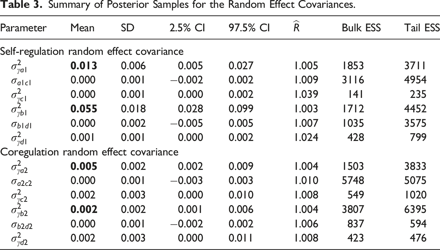
Summary of Posterior Samples for the Random Effect Covariances.

Parameter	Mean	SD	2.5% CI	97.5% CI	$\hat{R}$	Bulk ESS	Tail ESS
Self-regulation random effect covariance
$σ_{γ a 1}^{2}$	0.013	0.006	0.005	0.027	1.005	1853	3711
$σ_{a 1 c 1}$	0.000	0.001	−0.002	0.002	1.009	3116	4954
$σ_{γ c 1}^{2}$	0.000	0.001	0.000	0.002	1.039	141	235
$σ_{γ b 1}^{2}$	0.055	0.018	0.028	0.099	1.003	1712	4452
$σ_{b 1 d 1}$	0.000	0.002	−0.005	0.005	1.007	1035	3575
$σ_{γ d 1}^{2}$	0.001	0.001	0.000	0.002	1.024	428	799
Coregulation random effect covariance
$σ_{γ a 2}^{2}$	0.005	0.002	0.002	0.009	1.004	1503	3833
$σ_{a 2 c 2}$	0.000	0.001	−0.003	0.003	1.010	5748	5075
$σ_{γ c 2}^{2}$	0.002	0.003	0.000	0.010	1.008	549	1020
$σ_{γ b 2}^{2}$	0.002	0.002	0.001	0.006	1.004	3807	6395
$σ_{b 2 d 2}$	0.000	0.001	−0.002	0.002	1.006	837	594
$σ_{γ d 2}^{2}$	0.002	0.003	0.000	0.011	1.008	423	476

Group-level Average Tendency for Self-Regulation and Coregulation

First, we examined the average tendency (i.e., fixed effects) in dynamics on the two time scales. As a group, both males and females showed positive self-regulatory effects in both the physiological process on the second-by-second scale and the affective process on the daily scale (males: $β_{a_{10}} =$ 0.223 with CI = (0.174, 0.270), $β_{c_{10}}$ =0.083 with CI = (0.046, 0.121); females: $β_{b_{10}} =$ 0.299 with CI = (0.210, 0.388), $β_{d_{10}} =$ 0.083 with CI = (0.045, 0.121)). This showcased the natural continuity of physiological signals (IBIs in our example), and some day-to-day spillover of affect. However, the relation between any observation with its previous occasion was weaker (reflected by the magnitude of the self-regulation parameter) for the daily affective process than the more rapidly sampled, physiological process.

Unlike self-regulation, the overall between-partner effects were only perceptible in the daily affective process (males: $β_{c_{20}}$ =0.447 with CI = (0.370, 0.525); females: $β_{d_{20}} =$ 0.453 with CI = (0.371, 0.531)). On average, both males and females who had average dyad-level traits showed a tendency to approach their partners in their daily affect. That is, their daily relationship-specific affect was positively influenced by their partners’.

Between-Dyad Differences in Dynamics

Inspection of the regression coefficients on the individual self-regulation and coregulation parameters ( $β_{θ 1}$ ’s, $β_{θ 2}$ ’s and $β_{θ 3}$ ’s) did not support the effects of dyad-level attachment related anxiety, avoidance, or relationship quality on the process dynamics on these two time scales⁴.

Next, we examined the variation of the process dynamics across dyads. Results indicated reliable variation across dyads in all self-regulation and coregulation parameters in the physiological process ( $σ_{γ a 1}^{2}$ =0.013 with CI = (0.005, 0.027), $σ_{γ b 1}^{2}$ =0.055 with CI = (0.028, 0.099), $σ_{γ a 2}^{2}$ = 0.005 with CI = (0.002, 0.009), $σ_{γ b 2}^{2}$ =0.002 with CI = (0.001, 0.006)). This result implies meaningful differences between dyads in how the physiological signals of the dyad members self-regulated and adapted to those of their partners’, and such differences were not explained by the dyad-level trait variables we considered. However, we did not find meaningful between-dyad differences in dynamics from the daily process of affects⁵.

Associations Across Time Scales

The associations between corresponding parameters across the two processes were not apparent, as the covariance parameters $(σ_{a 1 c 1}$ , $σ_{b 1 d 1}$ , $σ_{a 2 c 2}$ , $σ_{b 2 d 2}$ ) were not different from zero. That is, there was no evidence indicating that individuals who showed higher or lower levels of self-regulation in one process would show similar or reversed tendencies in the other. This absence of association was also true for co-regulation.

For illustrative purposes, we discuss the interpretation of the covariance parameters in hypothetical terms. If a covariance parameter (say, $σ_{a 1 c 1}$ , the covariance between the male self-regulation parameters in the two processes) is positive, then individuals would show a similar tendency in the two processes. For example, those individuals in the sample who show higher-than-average self-regulation (so they recover faster than average after perturbation) in their physiological responses for the laboratory task would also show higher-than-average self-regulation in their daily affect (Figure 3). Alternatively, those individuals who are more likely to adapt to their partner in their physiological responses are also more likely to adapt in their everyday affective experiences (as in the case of a positive $σ_{a 2 c 2}$ , the covariance between the coregulation parameters representing female-to-male influence in the two processes, Figure 4). However, if a covariance parameter is negative, that means the processes are reversely associated. Individuals who are higher than average in one process would be lower than average on the same effect in the other process. Although we expected the two processes to reflect more or less the same dyadic characteristics, this latter hypothetical example remains a possible scenario.

Discussion

In this article, we utilized a Bayesian hierarchical dynamic model to assess whether dynamic parameters on one time scale were associated with their counterparts on another time scale. This model, as well as other hierarchical models on dynamics, can be used to statistically represent correlated processes on different time scales in situations where researchers believe an overarching construct or general pattern is responsible for manifesting both processes. To the best of our knowledge, this is novel in the literature. Utilizing Bayesian analytic tools also makes it relatively straightforward to extend the model to include more than two correlated processes and still fit the model in one step. We demonstrated the use of such hierarchical models with data from romantic partners collected with two types of measurements on two time scales. We represented each process with a VAR model and specified the dynamic parameters (self-regulation and coregulation) as mixed-effect parameters. The covariances between corresponding random effects, representing the association across time scales, were assessed in the model. Although we did not find support for such covariances, we discussed in theoretical terms how the parameters would be interpreted, had there been a covariance large enough.

In this article, we assumed that the physiological and affective interactions within romantic couples were similar processes with consistent patterns. Therefore, we only allowed the correlations between the corresponding dynamic parameters to be freely estimated and fixed other correlations to zero because we did not have strong reasons to do otherwise. However, this should not stop researchers from answering questions on potential associations represented by those other correlations. For example, would individuals who show stronger physiological self-regulation be more likely to influence their partners in their daily affect? This would be answered with a correlation parameter between one’s self-regulation parameter in physiological signals and their partner’s coregulation parameter (in that their partner is the receiver of influence) in daily affective states.

We chose the VAR model as an appropriate representation for the empirical data. Depending on a researcher’s theory and the phenomenon of interest, the VAR model part can be replaced by any other model deemed appropriate. The use of Bayesian hierarchical models needs not to be restricted to the VAR model we employed here, or even to dynamic models. It is also not required that the two models for the two processes be of the same form if theory suggests otherwise. For example, if theory suggests that greater self-regulation of daily emotions is associated with a faster decline of, say, neuroticism over years, then the model on the faster time scale can be an autoregressive model, and the one on the slower time scale can be a linear or exponential decay model, with the self-regulation parameter correlated with the decay rate parameter. The model-fitting method we adopted in this article is flexible in the models it can accommodate.

We would like to note that the term “coregulation” is studied in various dyadic phenomena (e.g., couples, parent-child, coworkers) without a clear and unified definition in the literature. In this article, we conceptualized coregulation as between-partner influences in the context of a VAR model, without specifying a direction for the effect. Other theoretical definitions of coregulation exist and different definitions result in different model choices. For example, Ferrer and Steele (2014) fitted five differential equation models to the daily affect data in couples, each based on a different theory and thus had a slightly different operationalization of coregulation (e.g., reference affect, predator-prey, mutualism). Another model relatively popular for dyadic emotions is the coupled damped oscillator model (e.g., Boker & Nesselroade, 2002; Butner et al., 2007). A thorough examination of the coregulation effect, however, is beyond the scope of this article.

In this article, we assumed that the imitation laboratory task captured the couples’ everyday interaction on a physiological metric. A previous study uncovered differences between tasks with this procedure, and the imitation task had the highest parameter estimates for coregulation among the three tasks (Ferrer & Helm, 2013). However, although evidence supported this task as reflective of some degree of interpersonal interaction between couples, it is unclear whether this kind of interaction reflects the normative physiological processes between partners in all couples, as the task instruction was made deliberately vague. Therefore, more investigation is needed regarding the potentially different dyadic physiological responses under laboratory stimuli and in their daily lives. Findings in the article must also be interpreted within the context of sampling limitations. Our relatively small sample was cisgender, heterosexual, and mostly white/Caucasian. In addition, no disability information was collected. Future research may examine these processes with larger and more diverse samples.

We would like to caution the readers again that, in the results of our empirical illustration, a few parameters had low ESS ( $β_{a_{13}},$ $β_{b_{11}}$ , $β_{b_{12}},$ and $σ_{γ c 1}^{2}$ ). A low ESS can sometimes be improved with more chains or more iterations per chain when fitting the model. When this does not help, one can also simplify the model by reducing some parameters or reparametrize. As the goal of our illustration was to demonstrate the use of the full model, we did not attempt to simplify and interpreted the results, but in practice, caution should be exercised with parameters that have low ESS.

In the previously published study by Ferrer and Helm (2013), the authors found a significant correlation between females' coregulation parameters in the physiological process and their daily affect. However, our analysis failed to replicate this finding. We would like to point out that although both the data in this article and those in Ferrer and Helm (2013) came from the same overarching study, the sample sizes were different as more data became available. Our sample size consisted of 29 couples, as opposed to the 15 in the previous article. Secondly, the one-step analysis in this article, compared to doing a similar analysis in two steps, benefits from the retention of uncertainty of the mixed effect coefficients, thus may result in more conservative errors/deviations and interval estimates.

In conclusion, the increasing availability of dense data together with developments in estimation procedures has made possible the formal evaluation of complex models across multiple time scales. In this article, we describe an example of a model examining the dynamics of two processes that rely on different measures and metrics, and unfold over different time scales. We hope this illustration motivates the use of more dynamic models that allow testing complex hypotheses and, ultimately, advance our understanding of social interactions.

Footnotes

Acknowledgement

We acknowledge the help and comments by the members of the Dynamics of Dyadic Interactions Project (DDIP) Lab at University of California, Davis, as well as Michael D. Hunter and the members of the Modeling of Developmental Systems (MODS) Lab at the Pennsylvania State University.

Funding

This study was supported by grants from the National Science Foundation (BCS-05-27766 and BCS-08-27021).

ORCID iD

Meng Chen

Open research statement

As part of IARR’s encouragement of open research practices, the authors have provided the following information: This research was pre-registered.

The data used in the research are available. The data can be obtained by emailing: eferrer@ucdavis.edu. The materials used in the research are available. The materials can be obtained at by emailing: mengc2013@gmail.com.

Notes

References

Beltz

A. M.

Molenaar

P. C.

(2016). Dealing with multiple solutions in structural vector autoregressive models. Multivariate behavioral research, 51(2–3), 357–373.

Bertenthal

B. I.

(2007). Dynamical systems: It's all about time. In Boker

Wenger

(Eds.), Data analytic techniques for dynamical systems (pp. 1–24). Erlbaum.

Boker

S. M.

Nesselroade

J. R.

(2002). A method for modeling the intrinsic dynamics of intraindividual variability: Recovering the parameters of simulated oscillators in multi-wave panel data. Multivariate Behavioral Research, 37(1), 127–160. https://doi.org/10.1207/S15327906MBR370106

Bowlby

(1982). Attachment and loss: Retrospect and prospect. American Journal of Orthopsychiatry, 52(4), 664–678. https://doi.org/10.1111/j.1939-0025.1982.tb01456.x

Brennan

K. A.

Clark

C. L.

Shaver

P. R.

(1998). Self-report measurement of adult attachment: An integrative overview. In Attachment theory and close relationships (pp. 46–76). The Guilford Press.

Bringmann

L. F.

M. L.

Vissers

Ceulemans

Borsboom

Vanpaemel

Tuerlinckx

Kuppens

(2016). Assessing temporal emotion dynamics using networks. Assessment, 23(4), 425–435. https://doi.org/10.1177/1073191116645909

Butler

E. A.

(2011). Temporal interpersonal emotion systems: The “TIES” that form relationships. Personality and Social Psychology Review, 15(4), 367–393. https://doi.org/10.1177/1088868311411164

Butner

Diamond

L. M.

Hicks

A. M.

(2007). Attachment style and two forms of affect coregulation between romantic partners. Personal Relationships, 14(3), 431–455. https://doi.org/10.1111/j.1475-6811.2007.00164.x

Carpenter

Gelman

Hoffman

M. D.

Lee

Goodrich

Betancourt

Riddell

Guo

(2017). Stan: A probabilistic programming language. Journal of Statistical Software, 76(1), 1–32. https://doi.org/10.18637/jss.v076.i01

10.

Chambliss

D. F.

Schutt

R. K.

(2018). Causation and experimental design. Making Sense of the Social World: Methods of Investigation, 120–149.

11.

Chen

Chow

S. M.

Hunter

M. D.

(2018). Stochastic differential equation models with time-varying parameters. In Continuous time modeling in the behavioral and related sciences (pp. 205–238). Springer.

12.

Cook

W. L.

Kenny

D. A.

(2005). The actor–partner interdependence model: A model of bidirectional effects in developmental studies. International Journal of Behavioral Development, 29(2), 101–109. https://doi.org/10.1080/01650250444000405

13.

Cook

W. L.

Snyder

D. K.

(2005). Analyzing nonindependent outcomes in couple therapy using the actor-partner interdependence model. Journal of Family Psychology, 19(1), 133–141. https://doi.org/10.1037/0893-3200.19.1.133

14.

Eason

E. G.

Carver

N. S.

Kelty-Stephen

D. G.

Fausto-Sterling

(2020). Using vector autoregression modeling to reveal bidirectional relationships in gender/sex-related interactions in mother-infant dyads. Frontiers in Psychology, 11, 1507–1507. https://doi.org/10.3389/fpsyg.2020.01507

15.

Feeney

B. C.

Kirkpatrick

L. A.

(1996). Effects of adult attachment and presence of romantic partners on physiological responses to stress. Journal of Personality and Social Psychology, 70(2), 255–270. https://doi.org/10.1037/0022-3514.70.2.255

16.

Felmlee

D. H.

Greenberg

D. F.

(1999). A dynamic systems model of dyadic interaction. Journal of Mathematical Sociology, 23(3), 155–180. https://doi.org/10.1080/0022250X.1999.9990218

17.

Ferrer

Helm

J. L.

(2013). Dynamical systems modeling of physiological coregulationin dyadic interactions. International Journal of Psychophysiology, 88(3), 296–308. https://doi.org/10.1016/j.ijpsycho.2012.10.013

18.

Ferrer

Nesselroade

J. R.

(2003). Modeling affective processes in dyadic relations via dynamic factor analysis. Emotion, 3(4), 344–360. https://doi.org/10.1037/1528-3542.3.4.344

19.

Ferrer

Steele

(2014). Differential equations for evaluating theoretical models of dyadic interactions. In Molenaar

P. C.

Lerner

Newell

K. M.

(Eds.), Handbook of developmental systems theory and methodology (pp. 345–368).

20.

Ferrer

Widaman

K. F.

(2008). Dynamic factor analysis of dyadic affective processeswith intergroup differences. In Card

N. A.

Selig

J. P.

Little

T. D.

(Eds.), Modeling dyadic and interdependent data in the developmental and behavioral sciences (pp. 107–137). Psychology Press.

21.

Fletcher

G. J.

Simpson

J. A.

Thomas

(2000). The measurement of perceived relationship quality components: A confirmatory factor analytic approach. Personality and Social Psychology Bulletin, 26(3), 340–354. https://doi.org/10.1177/0146167200265007

22.

Gelman

Rubin

D. B.

Others (1992). Inference from iterative simulation using multiple sequences. Statistical Science, 7(4), 457–472. https://doi.org/10.1214/ss/1177011136

23.

Gottlieb

(1991). Experiential canalization of behavioral development: Theory. Developmental Psychology, 27(1), 4–13. https://doi.org/10.1037/0012-1649.27.1.4

24.

Graber

E. C.

Laurenceau

J. P.

Carver

C. S.

(2011). Integrating the dynamics of personality and close relationship processes: Methodological and data analytic implications. Journal of personality, 79(6), 1403–1439.

25.

Hamaker

E. L.

Zhang

van der Maas

H. L. J.

(2009). Using threshold autoregressive models to study dyadic interactions. Psychometrika, 74(4), 727–745. https://doi.org/10.1007/s11336-009-9113-4

26.

Helm

J. L.

Sbarra

Ferrer

(2012). Assessing cross-partner associations in physiological responses via coupled oscillator models. Emotion, 12(4), 748–762. https://doi.org/10.1037/a0025036

27.

Kashy

D. A.

Kenny

D. A.

(1999). The analysis of data from dyads and groups. In Reis

H. T.

Judd

C. M.

(Eds.), Handbook of research methods in social psychology. Cambridge University Press.

28.

Kelley

H. H.

Holmes

J. G.

Kerr

N. L.

Reis

H. T.

Rusbult

C. E.

Van Lange

P. A.

(2003). An atlas of interpersonal situations. Cambridge University Press.

29.

Kelso

(1995). Dynamic patterns: The self-organization of brain and behavior. The MIT Press.

30.

Kuppens

Oravecz

Tuerlinckx

(2010). Feelings change: Accounting for individual differences in the temporal dynamics of affect. Journal of Personality and Social Psychology, 99(6), 1042–1060. https://doi.org/10.1037/a0020962

31.

LeDoux

(2003). The emotional brain, fear, and the amygdala. Cellular and Molecular Neurobiology, 23(4), 727–738. https://doi.org/10.1023/a:1025048802629

32.

Lewis

M.D.

Ferrari

(2001). Cognitive–emotional self-organization in personality development and personal identity. In Bosma

H.A.

Kunnen

E.S.

(Eds.), Identity and emotion: Development through self-organization (pp. 177-201). Cambridge University Press. https://doi.org/10.1017/CBO9780511598425.015.

33.

Mikulincer

Shaver

P. R.

(2019). Attachment orientations and emotion regulation. Current Opinion in Psychology, 25, 6–10. https://doi.org/10.1016/j.copsyc.2018.02.006

34.

Minuchin

(1985). Families and individual development: Provocations from the field offamily therapy. Child Development, 56(2), 289–302. https://doi.org/10.2307/1129720

35.

Nesselroade

J. R.

(1991). The warp and the woof of the developmentalfabric. In Visions of aesthetics, the environment & development: Thelegacy of Joachim F. Wohlwill (pp. 213–240). Lawrence Erlbaum.

36.

Newell

(1990). Unified theories of cognition. Harvard University Press.

37.

Oud

J. H. L.

Jansen

R. A. R. G.

(2000). Continuous time state space modeling. Psychometrika, 65(2), 199–215. https://doi.org/10.1007/bf02294374

38.

Palumbo

R. V.

Marraccini

M. E.

Weyandt

L. L.

Wilder-Smith

McGee

H. A.

Liu

Goodwin

M. S.

(2017). Interpersonal autonomic physiology: A systematic review of the literature. Personality and Social Psychology Review, 21(2), 99–141. https://doi.org/10.1177/1088868316628405

39.

Porges

S. W.

(2007). The polyvagal perspective. Biological Psychology, 74(2), 116–143. https://doi.org/10.1016/j.biopsycho.2006.06.009

40.

R Core Team (2018). R: A language and environment for statistical computing [computer software manual]. https://www.r-project.org/

41.

Roisman

G. I.

(2007). The psychophysiology of adult attachment relationships: Autonomic reactivity in marital and premarital interactions. Developmental Psychology, 43(1), 39–53. https://doi.org/10.1037/0012-1649.43.1.39.PMID:17201507

42.

Sbarra

D. A.

Hazan

(2008). Coregulation, dysregulation, self-regulation: An integrative analysis and empirical agenda for understanding adult attachment, separation, loss, and recovery. Personality and Social Psychology Review, 12(2), 141–167. https://doi.org/10.1177/1088868308315702

43.

Schwartz

R. M.

(1997). Consider the simple screw: Cognitive science, quality improvement, and psychotherapy. Jounral of Consulting and Clinical Psychology, 65(6), 970–983. https://doi.org/10.1037/0022-006x.65.6.970

44.

Shaver

P. R.

Mikulincer

(2002). Attachment-related psychodynamics. Attachment and Human Development, 4(2), 133–161. https://doi.org/10.1080/14616730210154171

45.

Stan Development Team (2020). RStan: the R interface to Stan (2.21.2. http://mc-stan.org/

46.

Stan Development Team (2022). Stan modeling language users guide and reference manual. Version 2.29 https://mc-stan.org

47.

Steele

J. S.

Ferrer

(2011). Latent differential equation modeling of self-regulatory and coregulatory affective processes. Multivariate Behavioral Research, 46(6), 956–984. https://doi.org/10.1080/00273171.2011.625305

48.

Steele

J. S.

Ferrer

Nesselroade

J. R.

(2014). An idiographic approach to estimating models of dyadic interactions with differential equations. Psychometrika, 79(4), 675–700. https://doi.org/10.1007/s11336-013-9366-9

49.

Torrisi

Lieberman

Bookheimer

S. Y.

Altshuler

L. L.

(2013). Advancing understanding of affect labeling with dynamic causal modeling. Neuroimage, 82, 481–488. https://doi.org/10.1016/j.neuroimage.2013.06.025

50.

Vehtari

Gelman

Simpson

Carpenter

Bürkner

P.-C.

(2020). Rank-normalization, folding, and localization: An improved for assessing convergence of MCMC. Bayesian Analysis, 16(2), 667–718. https://doi.org/10.1214/20-ba1221

51.

Zheng

Luo

Chen

(2020). Different effects of attachment anxiety and attachment avoidance on depressive symptoms: A meta-analysis. Journal of Social and Personal Relationships, 37(12), 3028–3050. https://doi.org/10.1177/0265407520946482

Assessing dynamical associations in dyadic interactions across multiple time scales via a Bayesian hierarchical vector autoregressive model

Abstract

Keywords

Process-Oriented Thinking in Relationship Research

Dynamic Modeling of Processes

Associations of Processes Across Different Time Scales

Modeling Association Between Patterns in Different Time Scales

Empirical Illustration: Couples’ Physiological and Affective Interactions

Method

Participants

Procedure

Laboratory Tasks

Daily Questionnaires

Measures

Cardiac Arousal

Relationship-Specific Affect

Dyad-Level Traits

Model and Analysis

Self-Regulation Parameters

Coregulation Parameters

Process Noise Parameters

Results

Group-level Average Tendency for Self-Regulation and Coregulation

Between-Dyad Differences in Dynamics

Associations Across Time Scales

Discussion

Footnotes

Acknowledgement

Funding

ORCID iD

Open research statement

Notes

References