
Abstract
In order to solve the hysteretic character of the piezoelectric material for application, the initial weight factors of the hysteretic units are calculated by the Preisach theory and the first-order reversal curves test data, a hysteretic Preisach model based on the improved fuzzy least square support vector machine (improved FLS-SVM) is established. In the established model, the fuzzy least square support vector machine is introduced to calculate more weight factors of the hysteretic units and the adaptive variable chaos immune algorithm is introduced to optimize the penalty factor and the kernel parameter of the FLS-SVM (the penalty factor c = 35 and the kernel parameter σ = 1.35 are obtained). Moreover, the quadratic polynomial interpolation method is used to eliminate the sawtooth phenomenon. The validity of established model reveals that fuzzy least square support vector machine method based on adaptive variable chaos immune algorithm (FLS-SVMAVCIA) is more accurate than FLS-SVM method according to application results of the real actuators (the absolute mean error of the FLS-SVMAVCIA model is less than 1 µm and its maximum error is less than 2 µm). As a result, the hysteretic phenomenon can be effectively eliminated by the hysteretic Preisach model based on the FLS-SVMAVCIA method.
Keywords
Introduction
There are many noise and vibration phenomena in the complicated mechanical and electrical systems.1–5 Noise and vibration in the complicated mechanical and electrical systems and their control still represent serious challenges to researchers, engineers, and constructors. Piezoelectric material is one type of crystalline materials, which has the ability to generate voltage between the two ends when the materials are under pressure,6,7 and the effect is called the positive piezoelectric effect. Relatively, when the piezoelectric materials are under the electric field, the materials can undergo deformations, which is to say the materials can convert the electrical energy into mechanical energy or mechanical movement, and the effect is called the inverse piezoelectric effect. The piezoelectric actuator8–10 based on the inverse piezoelectric effect is designed as the ideal driving components. The advantages of piezoelectric actuator are included as follows: high resolution of the displacement, strong driving force, high efficiency of electromechanical coupling, swift response and noiseless. 11 Therefore, the piezoelectric actuators are widely adopted in the realm of active control and vibration and noise reduction. However, the piezoelectric materials are of the inherent characteristics of hysteresis, nonlinearity, creep deformation, etc.12,13 These inherent characteristics lead to some undesirable results such as low control accuracy, non-repeatability in the engineering and the slow transient response of the materials. 14 As a result, it is difficult to employ piezoelectric actuators in industrial applications.
At present, there were some investigations on the hysteresis problem of the piezoelectric materials and researchers had proposed some of the hysteretic models such as Preisach model,15,16 multi-objective parameter optimization model, 17 Dahl model, 18 Bouc-Wen model, 19 etc. And the most widely used models are the Preisach model and its improved models. The principle of the Preisach model is based on the double integral, its integral item is the weight factor of the hysteretic unit. But the Preisach model is of its own imperfections such as the sawtooth phenomenon in the output curve of the Preisach model with insufficient computational discrete data points, the large output error, and the long computational time as the number of computational discrete data points is increased.
Therefore, some research on solving the hysteresis problem of the piezoelectric materials had been carried out. A neural network model for the identification of Preisach-type hysteresis was proposed and a hysteretic operator was introduced to transform the multi-valued mapping of hysteresis into a one-to-one mapping in Zhao and Tan. 20 A model based on the Preisach operator and analytic weight function was used to simulate the hysteretic large-signal behaviours in ferroelectric materials in Wolf et al. 21 Moreover, discrete Preisach model 22 and support vector machine (SVM)23,24 were applied to establish a hybrid model for piezoelectric actuators. In order to compensate a piezostage driven by piezoelectric stack actuators, the extended least squares support vector machines (LS-SVMs)25–29 were used to establish the domain of nonlinear modelling and control other nonlinear systems. 30 An improved hysteresis model 31 for magnetostrictive actuators was presented and the proposed four hybrid genetic algorithms (HGAs) were applied to identify parameters of the improved model.
The above research revealed that the hysteresis problem of the piezoelectric materials had been focused on the establishment of hybrid model based on fusions of Preisach model and artificial intelligence techniques such as neural network, SVM, LS-SVM and HGAs. However, the hysteresis problem of the piezoelectric materials was not resolved effectively.
Compared with other artificial intelligence techniques such as Gaussian process(GP),32,33 Bayesian regression, 34 neural networks (NNs), 35 Gaussian process mixed model (GPMM), 36 fuzzy least squares support vector machines (FLS-SVM) is of unique advantages such as requiring less modelling data, simple calculation and quick identification capacity in resolving the nonlinear and high dimension problems with small sample sets. Moreover, an adaptive variable chaos immune algorithm (AVCIA) is useful for global optimization of nonlinear and high dimension problems. Therefore, a novel idea is to use the FLS-SVM optimized by an AVCIA to effectively resolve the hysteresis problems of the piezoelectric materials, and new contributions in the paper are expressed as follows: (1) A hysteretic Preisach model based on the improved FLS-SVM was established; (2) The AVCIA was introduced to optimize the penalty factor and the kernel parameter of the FLS-SVM; (3) The hysteretic phenomenon was eliminated effectively by the hysteretic Preisach model based on the FLS-SVMAVCIA method. The research results reveal that the validity of the hysteretic Preisach model based on the improved FLS-SVM has been tested.
Identification of parameters of the Preisach hysteretic model based on the improved FLS-SVM
Theory of the generalized Preisach hysteretic model
The computational method of the generalized Preisach hysteretic model is through the double integral of the hysteretic factor, and the result of the method represents the character of the generalized Preisach hysteretic model. The mathematical relationship between the input and output can be expressed as

The principle of the hysteretic unit is shown in Figure 1.
Principle of hysteretic unit.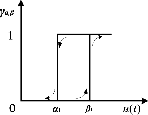
The output will not switch to 1 until the input of u(t) is greater than β1 when the input is increased. Similarly, the output will not switch to 0 until the input of u(t) is smaller than α1 when the input is decreased.
The hysteretic unit (α1, β1) presented in Figure 1 can also be expressed in the Preisach plane in which α and β are used as the coordinates and β ≥ α, and the schematic diagram is shown in Figure 2. The value ranges of α and β are between umin and umax, which are the minimum and maximum value of the input, respectively.
Hysteretic unit shown in α-β plane.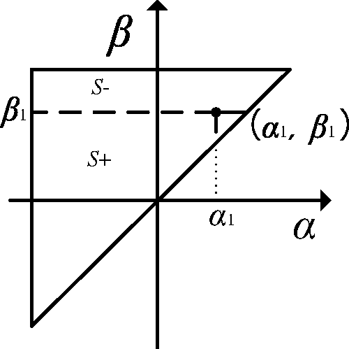
In the triangle area surrounded by α and β, the value of the weight function μ(α, β) is not equal to 0 and the value of the weight function μ(α, β) is equal to 0 at out of the triangle area. When the input voltage u(t) is increased, the horizontal axis whose value is equal to the input is moving up and the output of the hysteretic unit below the horizontal axis switches to 1. Contrastively, when the input voltage u(t) is decreased, the vertical axis whose value is equal to the input is moving to the left and the output of the hysteretic unit on the right of this vertical axis switches to 0. As shown in Figure 2, the value of the hysteretic unit in area S+ which β ≤ β1 and α ≤ α1 is equal to 1, the other area is equal to 0.
For discrete hysteretic model, the triangle area shown in Figure 2 will be divided into infinite units and each unit represents different (αi, βj). For example, if the input voltage signal is divided into n segments, then the total number of the hysteretic model is n(n + 1)/2, and the hysteretic model consists of the n(n + 1)/2 units which are connected in parallel. The distance between two hysteretic unit is 1/(n + 1). So when the n is increased gradually, the output of the discrete hysteretic model will be more precise. But with the increase of the n, the computation of the weight factor is more difficult, and this will lead to consuming more computational time. The discrete hysteretic model can be expressed as equation (2).

Thus, the output of the hysteretic model expressed as equation (2) is the weight sum of the hysteretic unit which is not equal to 0.
Improved FLS-SVM based on AVCIA
Theory of the FLS-SVM
SVM is a mechanical learning method which was developed by Vapnik 37 for solving problems of pattern recognition and regression based on the statistics theory. The FLS-SVM theory is based on the SVM, and the basic principle is depicted as follows38–40: The fuzzy theory is introduced into the SVM for constructing the corresponding objective function, and different fuzzy punishment weight coefficients are introduced into the samples so that the noise sample data can be eliminated.
The assumed sample data of the FLS-SVM model is expressed as follows

The λ(xi) represents the fuzzy rules of the characteristic parameters of sample data after fuzzification. And in the process of training the FLS-SVM, the λ(xi) represents the weight effect, which is different between the training data. There is no general guideline to follow to construct the fuzzy subjection function. According to Abad et al., 41 the method called the linear distance fuzzy subjection function construction is applied. The principle is expressed as follows: using the distance between the sample data and the class-center as the value of the subjection degree, so this is a linear function and the larger distance is, the bigger subjection degree is.
For the sample set {x1, x2, … , xn}, x0 is treated as the class-centre, r is treated as class-radius, and then


The function of subjection degree λ(xi) of the sample data can be expressed as equation (6).

The objective function of the FLS-SVM is modified after introducing the fuzzy subjection degree.


To solve the optimal problem which shows in equation (7), the Lagrangian factor ai (i = 1, 2, … , n) is introduced, and the corresponding Lagrangian function is expressed as equation (8).

In order to obtain the minimum of the objective function, making the partial derivative of the parameters w, ɛi, b, ai in equation (8) equal to 0, thus the equation (9) can be expressed as follows.
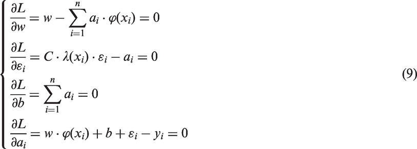
Eliminating the parameters w and ɛi, then the optimal problem is transferred into the problem of solving the linear system of equation (10).

Defining K(xi, xj) = ϕ(xi)ϕ(xj) and K(xi, xj) can be called the kernel function, thus equation (7) can be expressed as equation (11) which is the FLS-SVM model.

The commonly used kernel function is as follows: radial basis kernel function, polynomial kernel function, linear kernel function, sigmoid kernel function, etc. The widely used kernel function is the radial basis kernel function; due to that, the error of the function is smaller in application and the mathematical expression is written as equation (12).

Optimization of the radial basis kernel function by AVCIA
In order to solve the problems of the immune algorithm 42 which is easy to fall into local optimum in the whole iterative process and is of a low convergence rate in the late iterative process, an AVCIA is introduced to optimize the penalty factor C and kernel parameter σ.
Considering that the key to AVCIA is to determine the fitness function, the fitness function is selected as follow
The error function mean squared error (MSE) MSE is defined as the evaluation index of generalization performance of FLS-SVM:
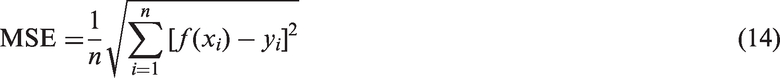
Figure 3 shows flow chart of optimizing parameters of FLS-SVM by AVCIA.
Flow chart of optimizing parameters of fuzzy least squares support vector machine by adaptive variable chaos immune algorithm.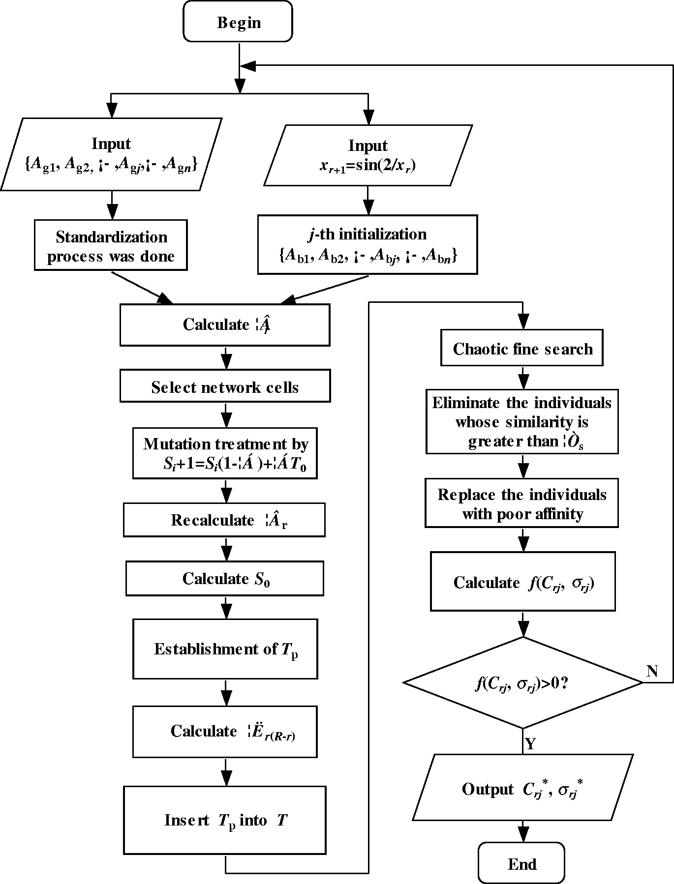
The concrete steps of AVCIA to optimize parameters of FLS-SVM are expressed as follows:


Fifteen per cent of the individuals whose fitness values are relatively large will be selected for chaotic fine search, and optimum individual is set as Y = (Y1, Y2, … , Yk), and the search interval of chaotic variables is narrowed as
43
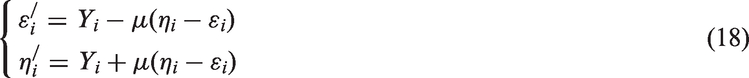
In order to ensure that the new range is not out of bound, some measurements are dealt with it as follows: if ɛi/<ɛi, ɛi/ = ɛi; if ηi/>ηi, ηi/ = ηi.
Therefore, vector Ti of Yi after reduction in the new interval [ɛ/
i
, η/
i
] can be determined using
The linear combination of Ti and Yi,
n
+1 will be expressed as a new chaotic variable and it is applied to chaotic fine search.

The adaptive control coefficient δi can be determined adaptively as follow

And then the individuals whose similarity is greater than σs in 10% of individuals with larger fitness value will be eliminated in the memory base.
Simulation verification of identification effect of FLS-SVM optimized by AVCIA
In order to verify the identification effect of AVCIA to optimize fuzzy least squares support vector machine(FLS-SVMAVCIA), three commonly used standard test (UCI) datasets are used in the experiments, and its identification effect is compared with the identification effect of the FLS-SVM and FLS-SVM optimized by particle swarm optimization algorithm (PSO) (FLS-SVMPSO).
Ripley dataset: The second Ripley dataset is adopted as the training set and the test set. The training set contains 800 samples (the number of positive class and negative class is 400, respectively), and the test set contains 1000 samples (the number of positive kind and negative kind is 500, respectively).
Monk dataset: The third Monk dataset in which noise points are added randomly is adopted, and the training set contains 800 samples (including 400 positive class and 400 negative class), the test set contains 1000 samples (including 500 positive class and 500 negative class).
Pima dataset: The total sample number of Pima dataset is 1800 (including 900 positive class and 900 negative class); 800 samples are randomly selected for training set and the remaining 1000 samples are set as test set in accordance with the dataset documents.
Optimal identification precision/%.
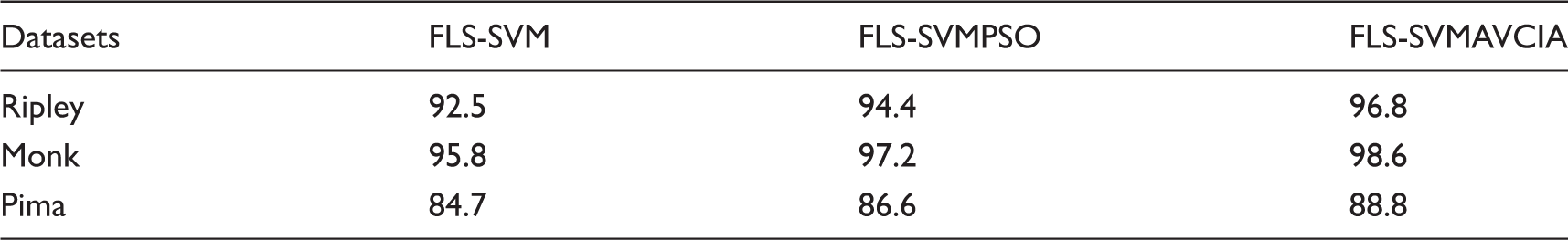
FLS-SVMPSO: fuzzy least square-support vector machine particle swarm optimization algorithm; FLS-SVM: fuzzy least square support vector machine; FLS-SVMAVCIA: fuzzy least square-support vector machine adaptive variable chaos immune algorithm.
Corresponding parameters correspond to identification precision.
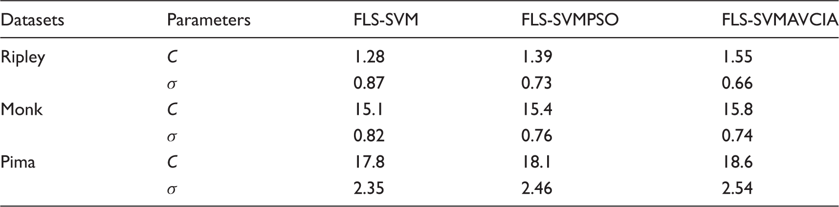
FLS-SVMPSO: fuzzy least square-support vector machine particle swarm optimization algorithm; FLS-SVM: fuzzy least square support vector machine; FLS-SVMAVCIA: fuzzy least square-support vector machine adaptive variable chaos immune algorithm.
As shown in Table 1, the FLS-SVMAVCIA proposed in this paper can effectively improve the identification precision of data in the dataset with noisy points and anomalous points.
CPU Time corresponds to identification precision datasets.
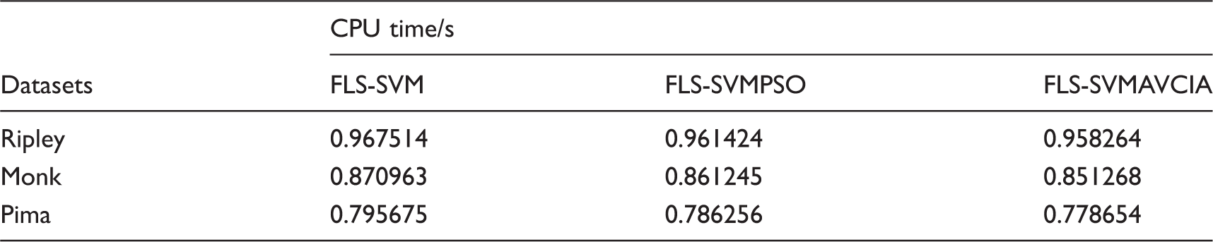
FLS-SVMPSO: fuzzy least square-support vector machine particle swarm optimization algorithm; FLS-SVM: fuzzy least square support vector machine; FLS-SVMAVCIA: fuzzy least square-support vector machine adaptive variable chaos immune algorithm.
Establishing of the Preisach hysteretic model based on the improved FLS-SVM
Establishing of the primary hysteretic piezoelectric model and its parameters optimization
The primary attributes of the piezoelectric actuator in paper are expressed as follows: the range voltage of driver is from 0 to120 V and the amplitude is 300 µm.
To establish the hysteretic piezoelectric model, the main task is to determine the weight coefficients of the hysteretic units. So the FORCs method is introduced to obtain the test data and compute the weight coefficients with these data. The input voltage is divided into six segments, so the value of n in FORCs curves.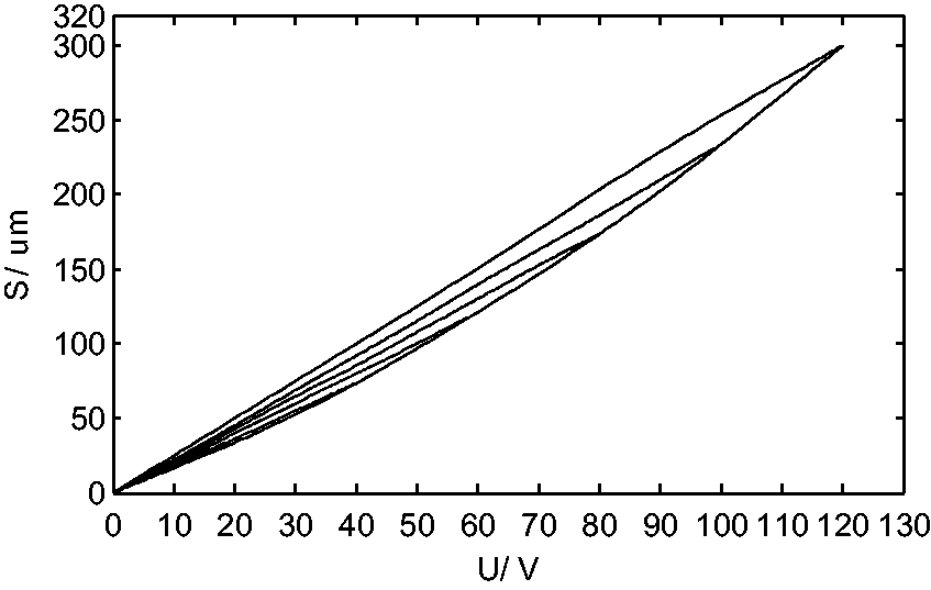
In Figure 4, the outer loop represents the voltage–displacement diagram, while input increases from 0 V to 120 V and then decreases to 0 V. The inner loop represents the voltage–displacement diagram while input increases from 0 V to 20 V, 40 V, 6 0 V, 80 V and 100 V, respectively, and then decreases to 0 V. From Figure 4, it can be concluded that the piezoelectric actuator in paper has a large hysteresis phenomenon. If the actuator is used directly, there are problems that the accuracy cannot be controlled and some large errors will appear.
In order to calculate the initial weight factors based on the test data, the simplified model is introduced. According to equation (1), the integrand is the weight factor. So a suitable weight factor value can be treated as a mean value in the integration domain that is divided into some units. Product values of mean weight factor values and the corresponding areas are treated as the total value of output and the mean weight factor value is expressed as the weight matrix elements in equation (2). Thus, equation (2) can be rewritten as

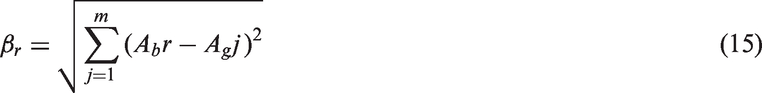
Before applying the FLS-SVMAVCIA method, assuming the coordinate of each unit’s centroid according to the element in matrix
The initial mean weight factor value is obtained based on the FORCs curves in Figure 5 and the value matrix is shown as
Curve of the fitness function.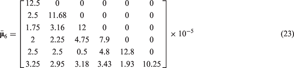
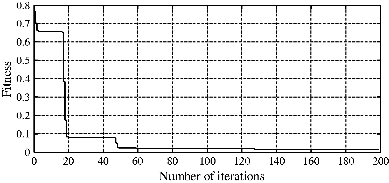
Finding the centroid of initial weight value of each unit in α-β plane, the coordinate of each centroid was calculated. Using the coordinate of each centroid as the input of the FLS-SVMAVCIA method and using the mean weight value of each unit as the output of the FLS-SVMAVCIA method, the model is trained and established. Applying the radial basis function as the kernel function, but the penalty factor c and kernel parameter σ must be optimized in the process of training due to the effect on the accuracy of the training model.
Figure 5 shows the curve of the fitness function in the process of parameters optimizing. From Figure 5, the value of fitness function is getting smaller when the iteration is increased, and finally the value of fitness function attains the required precision.
The penalty factor c and kernel parameter σ are obtained after the AVCIA optimization, c = 35, σ = 1.35. Thus, the parameters of the FLS-SVMAVCIA method are determined and the calculated model of the hysteretic model is established.
In order to solve more mean weight value, taking n = 12 which divides the α-coordinate and the β-coordinate into 12 segments, the interval is 10 V. Then centroid coordinates of each unit are calculated. The 78 calculated coordinates are used as the input of the FLS-SVMAVCIA method, then the 78 mean weight values is calculated. The result of the calculation is shown in Figure 6.
Calculated mean weight values.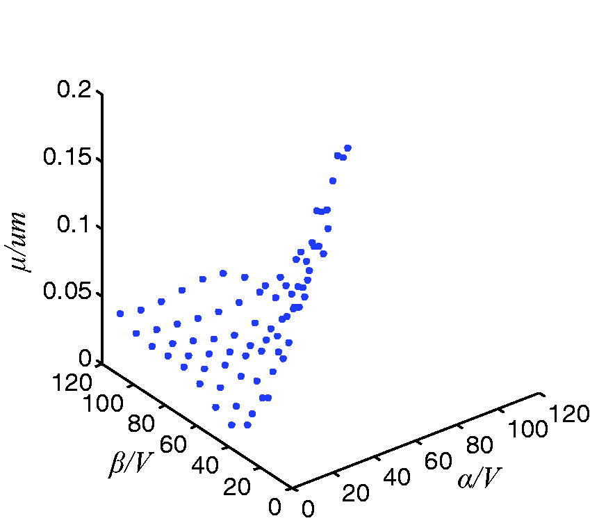
For obtaining the weight value which can be used in the discrete hysteretic model, it is important to multiply the mean weight value with the corresponding area. Thus, the initial piezoelectric hysteretic model is established.
Improvement of the initial piezoelectric hysteretic model
There is a disadvantage according to the theory of the discrete Preisach hysteretic model. The output of the discrete Preisach hysteretic model is toothed and the phenomenon is much more severe especially when the number of hysteretic units is small. In order to eliminate the inherent disadvantages of the toothed phenomenon, the interpolation method is introduced, thus the output curve of the model could be smooth and precise.
In order to compute the output of the hysteretic unit whose input is not on the specific voltage that was divided by 12 segments, the quadratic polynomial interpolation method is introduced to calculate the output of the model. Assume at one time, the input voltage is increased but the voltage value is not equal to the specific voltage, the quadratic polynomial interpolation can be expressed as

To obtain the values of the undetermined coefficients A0, A1, A2, three values of β are needed. Assuming that the input voltage u(t) is between value βq and value βq+1, then the β equals to βq-1, βq, βq+1 and the corresponding output f(βq-1), f(βq), f(βq+1) are obtained from the discrete Preisach hysteretic model, respectively; this leads to
The above equation reveals that q must be greater than or equal to 1. When the input voltage is less than β1, the quadratic polynomial interpolation method is not used to compute the output of the hysteretic unit because two values of the input voltage are just obtained. And the linear interpolation method is introduced to compute intermediate value between two values of the input voltage.
The undetermined coefficients A0, A1 and A2 are determined through equation (25) and the determined A0, A1 and A2 can be put into equation (24) to establish the polynomial interpolation model. So the output of the hysteretic model is known when the input is u(t) to equation. (24). Similarly, when the input voltage is decreased, the following interpolation equation can be obtained

The determination of B0, B1 and B2 is the same as the determination of A0, A1 and A2.
The final hysteretic piezoelectric model is obtained after combining with the polynomial interpolation. The toothed phenomenon is eliminated and the accuracy of the model is better. Figure 7 shows the comparison of the outer loops between the unimproved discrete Preisach hysteretic model and the improved one.
Comparison between unimproved and improved model. 1- the output of the hysteretic piezoelectric model which combines with the polynomial interpolation; 2- the output of the discrete Preisach hysteretic model.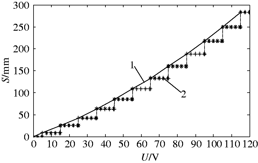
In Figure 7, the output of the hysteretic piezoelectric model combined with the polynomial interpolation is improved, and the output of the discrete Preisach hysteretic model is unimproved. The comparison of the figure suggests that the curve of the output is smoother after combining with the polynomial interpolation than that without the polynomial interpolation, so the method of the polynomial interpolation has a good effect on the discrete hysteretic piezoelectric model.
Validating of the hysteretic piezoelectric model
In order to validate the piezoelectric hysteretic model, the simulated model and the test platform are established. The MATLAB/Simulink software is used to establish the simulation model of the piezoelectric hysteretic model. The simulation model consists of two main modules, which are the discrete Preisach hysteretic model and the polynomial interpolation model. Moreover, 78 mean-weighted values are calculated after the α-coordinate and the β-coordinate are divided into 12 segments with the interval of 10 V and then 78 calculated coordinates are used as the inputs of the FLS-SVM. Therefore, the discrete Preisach hysteretic model consists of 78 Relay models which are connected with each other in parallel, the parameters of the Relay models are the values of weight factors calculated in “Establishing of the primary hysteretic piezoelectric model and its parameters optimization”. The polynomial interpolation model consists of equations in “Improvement of the initial iezoelectric hysteretic model” and the changing rate of the input. Figure 8 shows the connection of the computational model, where [A] represents the calculated median which can be transferred from the discrete hysteretic Preisach model to the polynomial interpolation model through “go to” module.
Simulink model of the piezoelectric hysteretic model.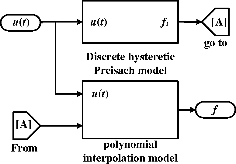
In order to meet the demands of contrast, the Preisach hysteretic model based on the FLS-SVM is established and the corresponding Simulink model is constructed, the principle and the steps of the constructing are similar to that of the FLS-SVMAVCIA. And Figure 9 shows the comparison diagram of the outer loops with different methods of FLS-SVM, FLS-SVMAVCIA and the test data.
Testing data and the simulation data. 1-The testing data; 2-the simulated data of the FLS-SVMAVCIA model; 3-the simulated data of the FLS-SVM model.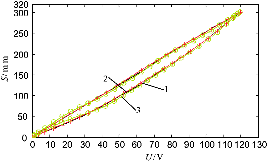
In Figure 9, it can be concluded that the error of the FLS-SVM model is large most of the time and the error of the FLS-SVMAVCIA model is smaller than that of the FLS-SVM model. Therefore, the capability of the FLS-SVMAVCIA model to fit the test data is very well.
As shown in Figure 10, the errors of the fitted curve by using of the FLS-SVMAVCIA method are very small and the maximum error of the curve is about 2.2 µm, so it is a good method to solve the hysteretic problem.
Error of the curve fitting. (a) Error of the bottom curve. (b) Error of the upper curve.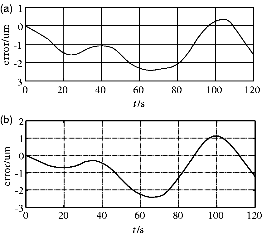
Comparison between simulated model and the test data in inner loop.
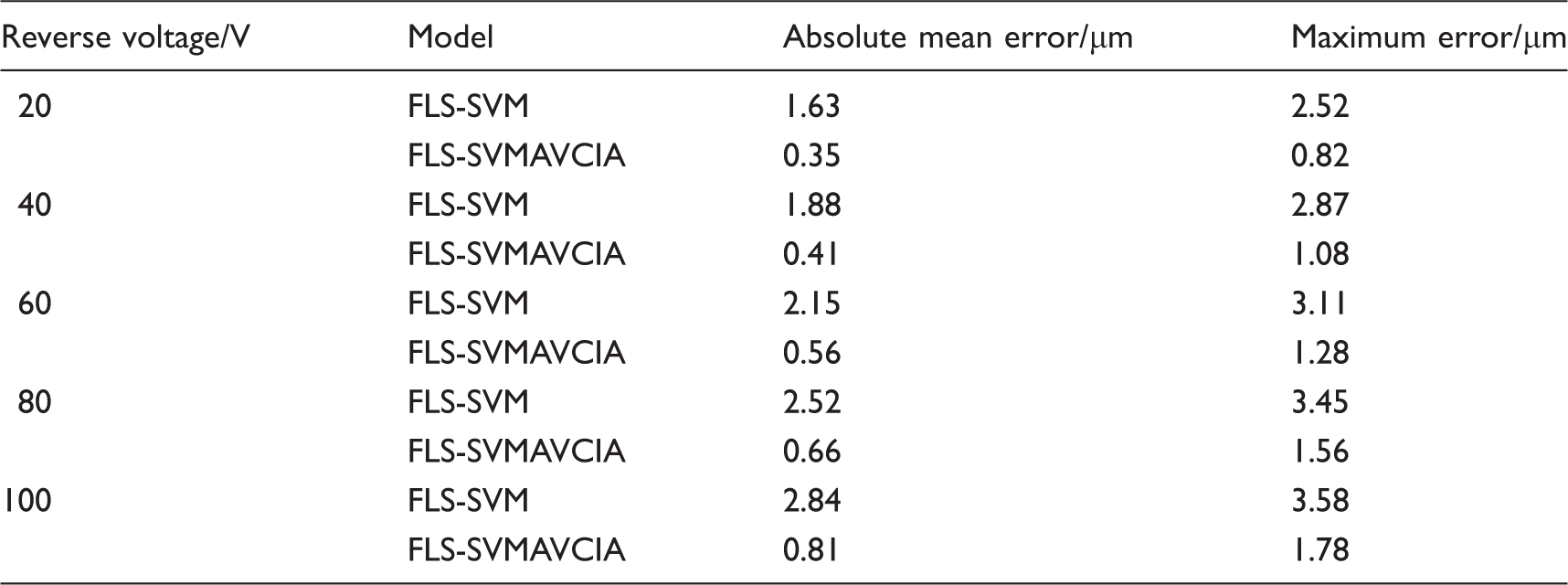
FLS-SVM: fuzzy least square support vector machine; FLS-SVMAVCIA: fuzzy least square-support vector machine adaptive variable chaos immune algorithm.
From Table 4, the absolute mean error and the maximum error of the FLS-SVM model are large, but the absolute mean error of the FLS-SVMAVCIA model is less than 1 µm and the maximum error of the FLS-SVMAVCIA model is less than 2 µm. So the hysteretic model based on the FLS-SVMAVCIA has a good fitting under the inner loop condition.
Through the comparison, the output of hysteretic model based on the FLS-SVMAVCIA has the same effect to the output of the real piezoelectric actuator, so the parameters identification of the hysteretic Preisach model based on the improved FLS-SVM in the paper is an effective method.
Conclusions
Based on the FORCs, the obtained 78 weight factors are used as the input of the FLS-SVM in the training model, the AVCIA is used to optimize the FLS-SVM, a method of FLS-SVMAVCIA is established to calculate the weight factors of the piezoelectric hysteretic model. Simulink is applied to establish the piezoelectric hysteretic model with FLS-SVMAVCIA method, the comparison results show that the hysteretic Preisach model based on the FLS-SVMAVCIA method is an effective method to eliminate the hysteretic phenomenon. The potentiality of the paper is the benefit for the development and usage of the piezoelectric actuators and the development of the precise control engineering. In further work, the frequency factor should be considered, especially at the working frequency range of the actuators.
Footnotes
Declaration of conflicting interests
The author(s) declared no potential conflicts of interest with respect to the research, authorship, and/or publication of this article.
Funding
The author(s) disclosed receipt of the following financial support for the research, authorship, and/or publication of this article: The authors would like to acknowledge Project (9140A2011QT4801) supported by weapons and equipment pre-research fund and the National Studying Abroad Foundation Project (No.201208430262) supported by the China Scholarship Council.