Lumped parameter modelling and methodology for extraction of model parameters for an electrodynamic shaker

Abstract

Shakers are widely used to simulate the vibrations for academic research, as well as for product testing. Thus, there is a significant necessity to study them in detail. Amongst the different types of shakers being used, the electrodynamic shaker is by far the most versatile. However, limited work has been done with regard to their integrated electro-mechanical modelling. In this work, we have developed a mobility-based lumped parameter model of an electrodynamic shaker and also a method to measure its various electrical and mechanical parameters using non-destructive and easy to use methods. Towards meeting the latter goal, we conducted experiments to determine the shaker table’s impedance and transfer functions, and used these data for subsequent parameter extraction. Such a model was later validated experimentally. Finally, we predicted the response of the shaker under loaded and unloaded conditions, and confirmed their validity through actual experimental data.

Introduction

Electrodynamic shakers are extensively used for product evaluation, stress screening, squeak and rattle testing, modal analysis and study of whole body vibrations. When a product is mounted on an electrodynamic shaker table, the shaker and product become closely-coupled, i.e. the response of electrodynamic shaker is influenced by the characteristics of product mounted on it and vice-versa. Thus, to accurately understand the performance of products at different frequencies, understanding of behaviour of electrodynamic shaker is very important.

Here, an electrodynamic shaker is modelled as a lumped parameter system. Using such an approach, the assembly of shaker and mounted product is converted into an analogous electrical model using the mobility analogy. Next, different parameters of this model have been extracted non-destructively using the experimental data. Finally, a comparison of shaker’s predicted response with experimental observations has been made.

Analogies used to represent mechanical systems using electrically equivalent circuits have been explained in Beranek ¹ and Rossi. ² Small and Thiele have used such equivalences to define different parameters of a loudspeaker and have shown the similarity of response curves of loudspeaker with those of electrical filters. They have also explained how different parameters of loudspeaker can be experimentally extracted. Yorke ³ has discussed some experimental techniques to measure different electrical and mechanical parameters of electrodynamic transducers and has presented some methods to identify the electrical parameters of electrodynamic transducers. Lang and Synder ⁴ have developed rudimentary electromechanical model of electrodynamic shaker and used it to predict its vibrational modes and also effects of its isolation from ground on its performance. Lang ⁵ has also presented a method to measure the mechanical parameters of small electrodynamic shakers using it as vibration sensor. Smallwood ⁶ has characterised an electrodynamic shaker as a two-port network with its input variables being voltage and current, and output variables being acceleration and force. Using such an approach, he characterised shakers as devices with 2 × 2 impedance matrix. Flora and Grundling ⁷ have shown how different mechanical parameters of electrodynamic shakers can be extracted from the ratio of shaker’s acceleration and inflowing current. The shaker model can be used for performance prediction and virtual shaker testing ⁸ using different commercial packages such Simulink, Orcad, and LMS Imagine.Lab.

This article is based on the work done by the author Puri ⁹ in her Master’s thesis.

Lumped parameter modelling of a medium sized electrodynamic shaker

Lumped parameter modelling has been successfully used for modelling a range of dynamic systems from vehicle suspensions^10–12 to buildings. ¹³ We have used a similar method to model the behaviour of a medium-sized electrodynamic shaker. Typically, such shakers have two sub-assemblies: a body and an armature assembly. Its body is made up of a top plate, centre pole, bottom plate and field coils. When DC current is supplied to the field coils, it produces radial magnetic flux which cuts across the armature coil. The armature assembly is a cylindrical coil wound on a stiff and ribbed structure. Armature assembly is suspended in the air gap between the centre pole and the top plate. This is shown in Figure 1. When varying electric signal is fed to the armature coil, the armature assembly vibrates. To prevent lateral motion of the armature assembly, flexures connecting armature assembly and body are designed to provide high lateral stiffness. When electric current flows in the armature coil, the body of the shaker experiences equal and opposite forces. To reduce dynamic forces transmitted to the ground, the body of shaker is isolated from the ground through an isolation system.

Figure 1.

Section view of medium-sized electrodynamic shaker.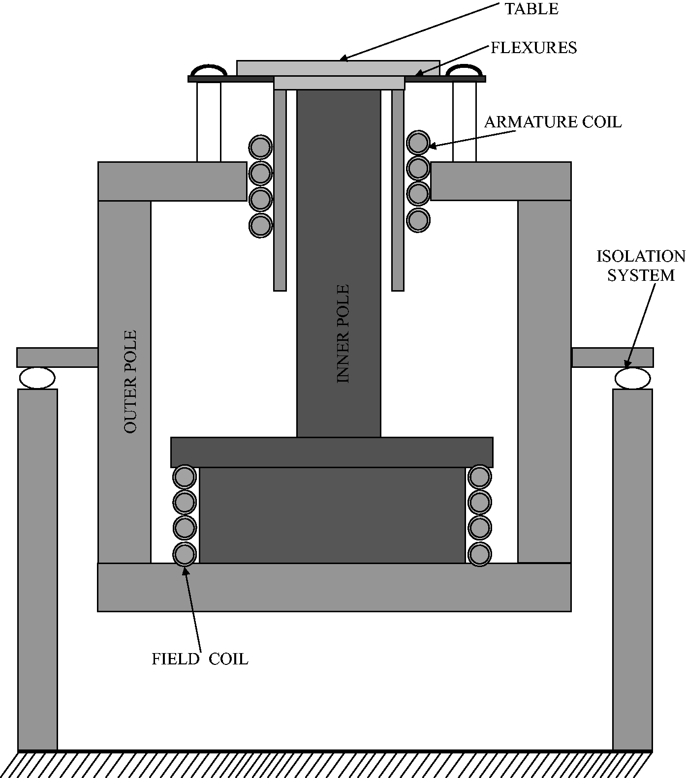

Electrodynamic shaker is an electro-mechanical system. On its electrical side, it has an armature coil with resistance, R_E, and inductance, L_E while the mechanical portion of the shaker maybe modelled as three masses, three springs and three mechanical resistors. Firstly, the shaker’s body of mass M_b, is connected to the ground through a spring of compliance C_b and a dashpot with a mechanical resistance of value R_b. The shaker’s body is also connected to the assembly of shaker table and armature coil, through a suspension spring with compliance C_ms and a mechanical resistance of value R_ms. Finally, the armature coil is adhesively connected to the shaker body. This bond has a finite stiffness, and it also provides some damping. At high frequencies, the armature coil and the shaker table no longer necessarily move as a single rigid body. Thus, in the lumped parameter model, the shaker table is coupled on its other side to an armature coil of mass M_c, via a spring of compliance C_c and a dashpot having mechanical resistance value of R_c. A schematic of such a mechanical system is shown in Figure 2.

Figure 2.

Lumped parameter model of the mechanical part of medium-sized electrodynamic shaker.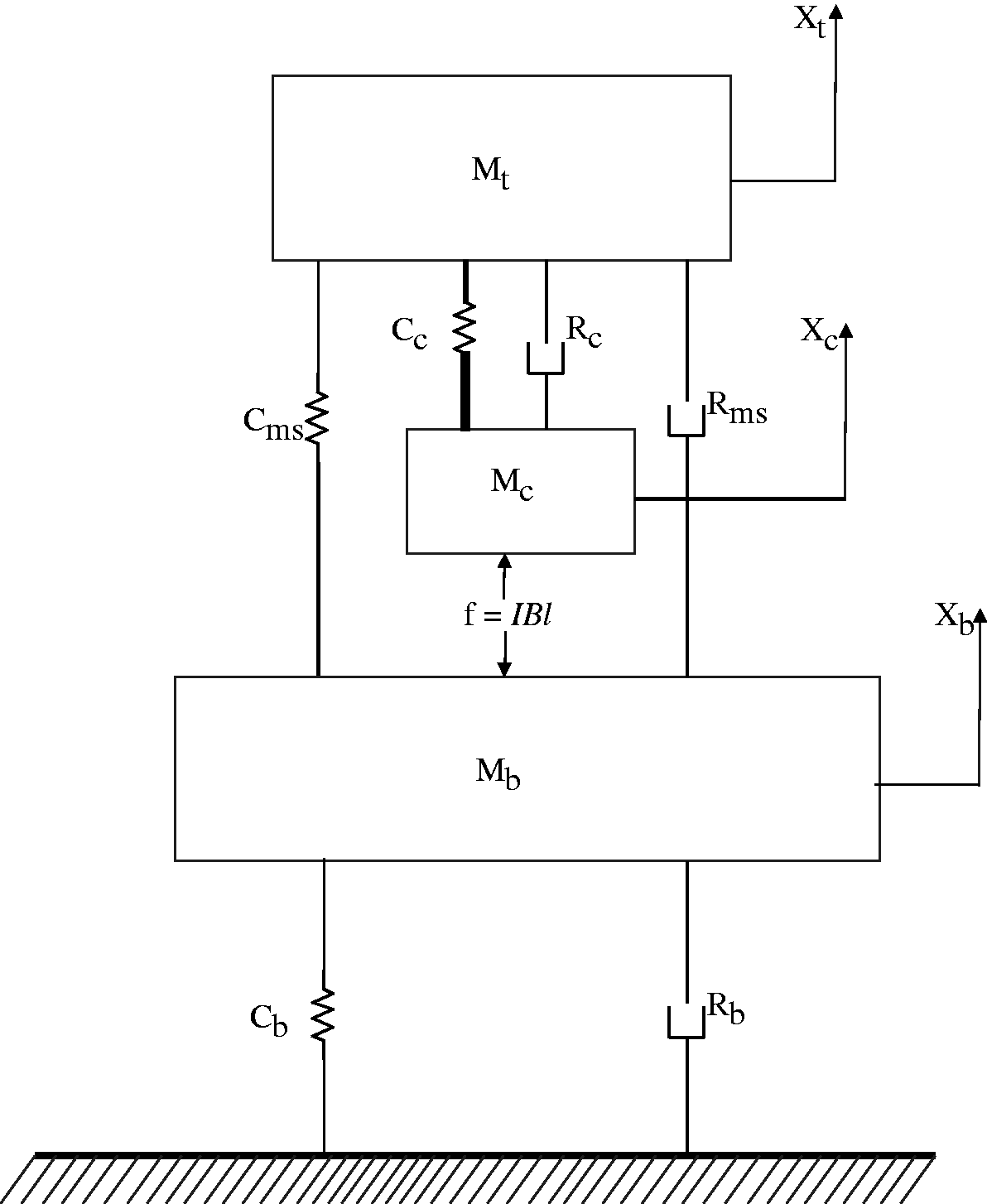

In Figure 2, three degrees of freedom are depicted. These are displacement of shaker body X_b, shaker table X_t and armature coil X_c, with respect to fixed ground. Also shown in this figure is the excitation force IBl, which acts on masses M_c and M_b simultaneously.

When the armature coil moves in a magnetic field, an electromotive force is generated which is directly proportional to the relative velocity of armature coil, $\stackrel{·}{X\text{c}}$ with respect to that of the shaker body, $\stackrel{·}{X\text{b}}$ . Thus, the value of the back e.m.f. generated due to the motion of armature coil is $\mathrm{Bl}(\stackrel{·}{X\text{c}}-\stackrel{·}{X\text{b}})$ where Bl is defined as the force factor.

Figure 3(a) and (b) depicts equivalent electrical models of electrical and mechanical parts of shaker based on mobility analogy. These two models are finally integrated into one single model as shown in Figure 3(c). In this model, we use a controlled current source, to apply equivalent reaction force IBl on the shaker’s body. In the model, we also use a voltage controlled voltage source to measure the voltage difference between the active terminals of M_c and M_b, and generate an equivalent voltage difference across the terminals of the transformer to actually simulate back emf.

Figure 3.

(a) Lumped model of electrical part of shaker. (b) Lumped model of mechanical part of shaker. (c) Overall lumped parameter model for the electrodynamic shaker.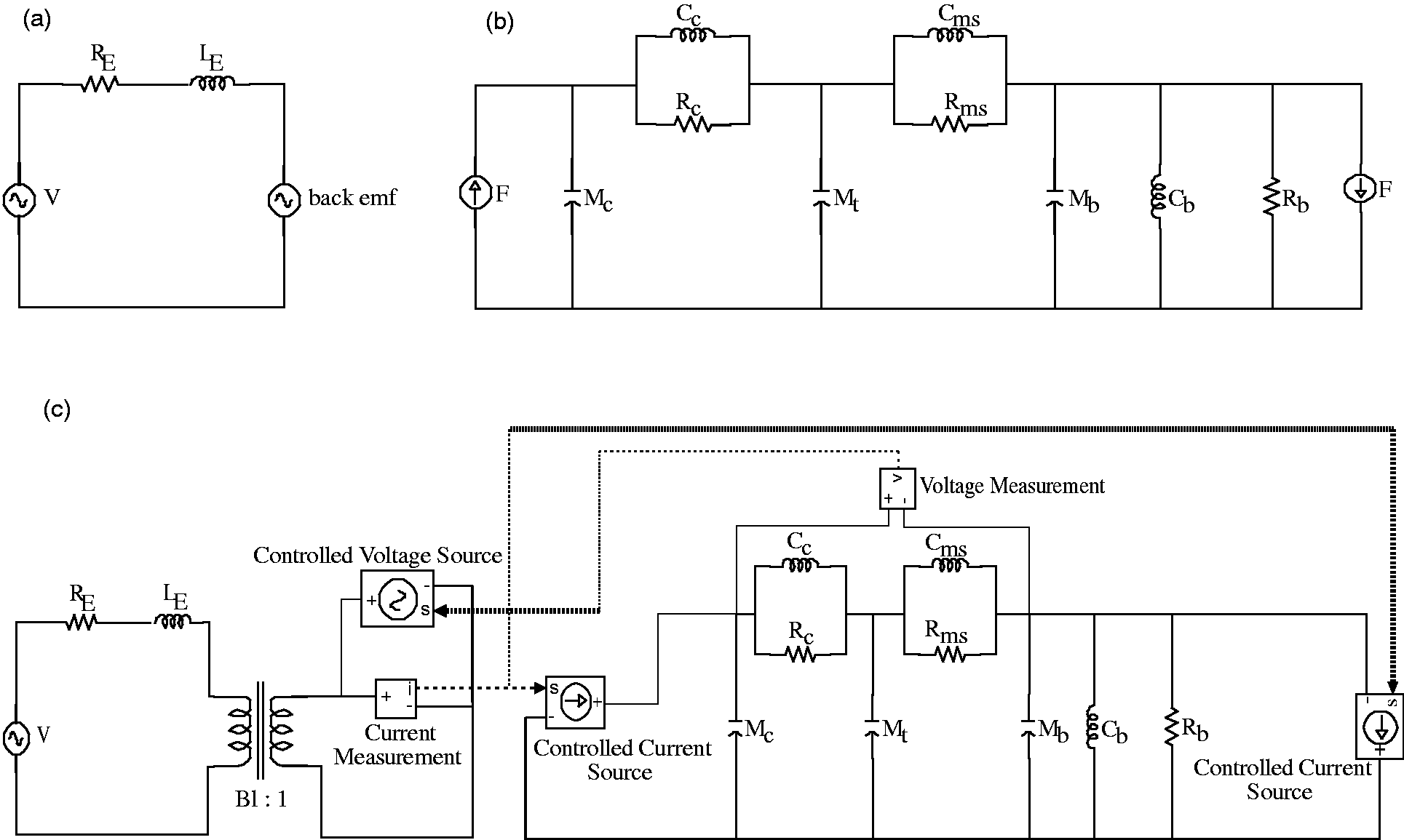

Methodology for experimental determination of different model parameters

The lumped parameter model shown in Figure 3(c) has three degrees of freedom. This is consistent with the fact that there are three principal vibration modes which dominate a shaker table’s operating characteristics. These are:

Isolation mode – The isolation mode occurs at very low frequencies. In this mode, armature assembly and the body of shaker vibrate as one single rigid body.

Suspension mode – This mode manifests at frequencies at least an order of magnitude higher than the isolation mode. In this mode, the armature assembly moves relative to the body of shaker.

Coil mode – At very high frequencies, the armature coil and the table of the shaker may move out of phase, and thus severe stresses may develop in the cylindrical structure of the shaker. Because of this, electrodynamic shakers are rarely used at frequencies exceeding coil mode resonance. This resonance associated with coil mode is also known as armature resonance.

In this work, we exploit the unique operating traits of the system in the vicinity of these modes to identify different model parameters.

Determination of mechanical parameters M_ms, C_ms, and R_ms

These parameters may be determined by analysing the response of shaker around its suspension mode resonance. In the neighbourhood of this resonance, many of the model elements as shown in Figure 3(c) have little influence on the system response, and hence may be removed from the circuit. Typically, the resonance point of armature coil exceeds suspension resonance by approximately two orders of magnitude. This is because the compliance of the armature coil, i.e. C_c, is very small compared to the suspension compliance, C_ms. Thus, in the region of suspension resonance, the impedance offered by C_c, may be ignored. Also, at frequencies significantly higher than isolation frequency, impedance offered by M_b, i.e. 1/(ωM_b) is negligible since M_b is very large. Further, armature coil inductance, i.e. L_E may be omitted because compared to R_E, the impedance offered by L_E is very small up to frequency values in the neighbourhood of suspension resonance. For instance, at 25 Hz, which is where we expect the suspension resonance of shaker under study, the impedance offered by L_E is 0.01575 Ω, while the expected value of R_E is 0.4 Ω. Thus, the simplified model of the shaker assembly as shown in Figure 4(a) may be used to find parameters M_ms, C_ms and R_ms.

Figure 4.

(a) Simplified equivalent electrical model of the shaker around suspension resonance. (b) Equivalent electrical model of the shaker above suspension resonance. (c) Equivalent electrical model of the electrodynamic shaker for ω > 10 ω_s. (d) Simplified model of the electrodynamic shaker at very high frequencies.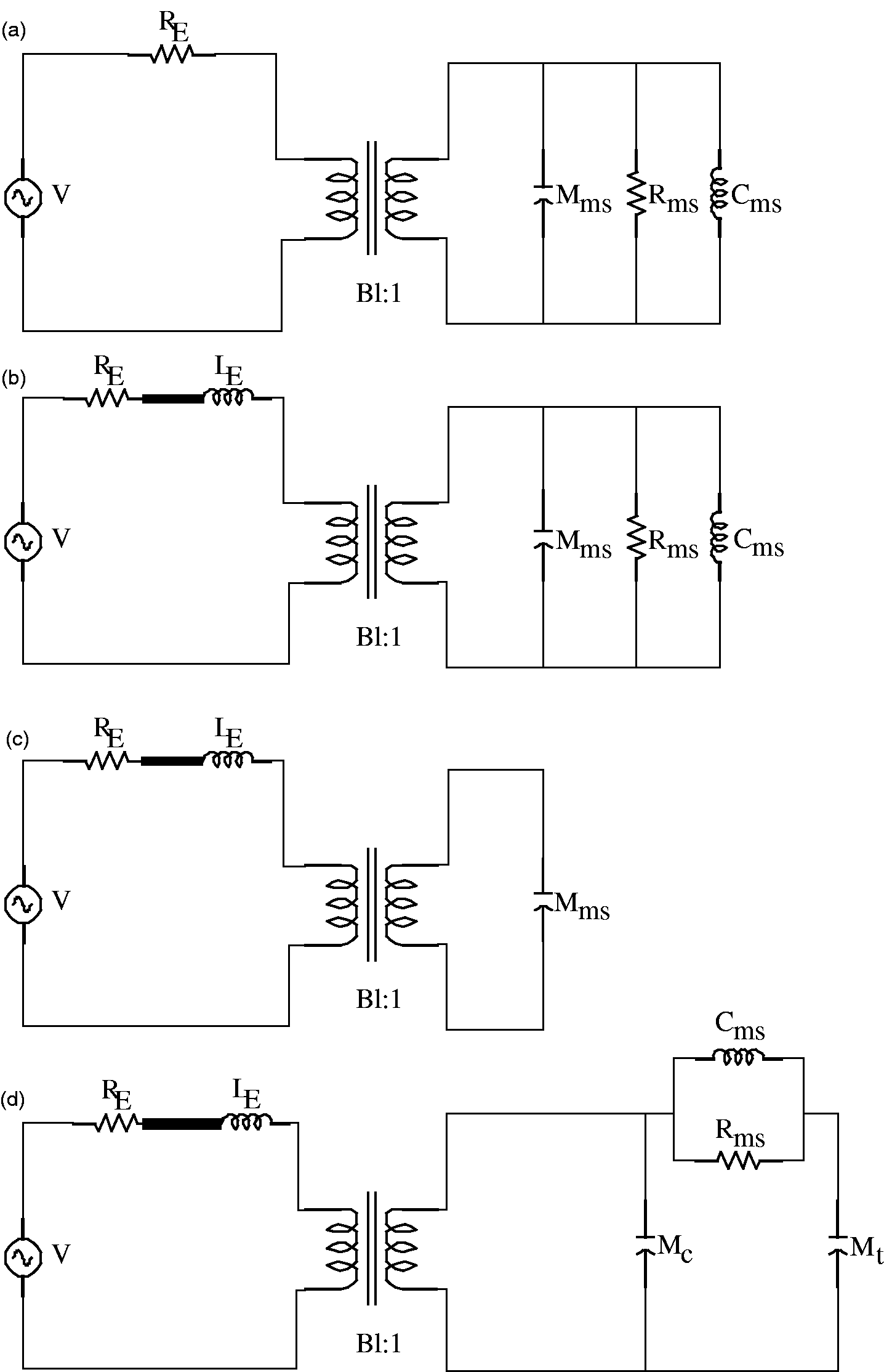

Since the simplified model as shown in Figure 4(a) has one degree of freedom, we use the added mass method to calculate the values of M_ms and C_ms. For such a model, the expression for impedance Z across terminals of the armature coil is

$$Z=R\text{E}+R\text{ms}(\mathrm{Bl})2(\frac{\text{j}\omega C\text{ms}}{\text{j}\omega C\text{ms}+(1-\omega 2M\text{ms}C\text{ms})R\text{ms}})$$

(1)

$\text{At}\omega =\frac{1}{\sqrt{M\text{ms}C\text{ms}}}$ , which is the point of suspension resonance, Z becomes purely real. Thus, the suspension resonance corresponds to the condition when imaginary impedance across terminals of armature coil is zero. This fact may be used to experimentally determine suspension resonance frequency for a bare table (ω_s1) and for a table loaded with mass ‘m’ (ω_s2). From ω_s1 and ω_s2, the mass of armature assembly and the compliance of armature suspension are calculated as follows

$$\omega \text{s}1=\frac{1}{\sqrt{M\text{ms}C\text{ms}}}\text{and}\omega \text{s}2=\frac{1}{\sqrt{(M\text{ms}+m)C\text{ms}}}$$

(2)

On solving equation (2)

$$M\text{ms}=\frac{{\omega }_{\text{s}2}^{2}m}{({\omega }_{\text{s}1}^2-{\omega }_{\text{s}2}^2)}\text{and}C\text{ms}=\frac{1}{({\omega }_{\text{s}1}^{2}M\text{ms})}$$

(3)

Also, at suspension resonant frequency, the value of impedance across terminals of armature coil is

$$Z=R\text{E}+R\text{ms}(\mathrm{Bl})2$$

(4)

Equation (4) may be used to determine the value of suspension responsiveness, R_ms, if parameters Z, R_E, and Bl are known.

Determination of electrical parameters R_E and L_E

Beyond suspension resonance, the impedance due to inductance of armature coil becomes somewhat appreciable and thus the equivalent electrical circuit for the shaker is shown in Figure 4(b). For such a system, the expression for impedance of the mechanical portion of the system, Z_mech, is

$$Z\text{mech}=\frac{\text{j}\omega R\text{ms}C\text{ms}(\mathrm{Bl})2}{R\text{ms}(1-\omega 2M\text{ms}C\text{ms})+\text{j}\omega C\text{ms}}$$

(5)

Further, the imaginary part of Z_mech can be expressed as

$$\text{Im}(Z\text{mech})=\frac{\omega R_{\text{ms}}^{2}C\text{ms}(1-\omega 2M\text{ms}C\text{ms})(\mathrm{Bl})2}{(R\text{ms}(1-\omega 2M\text{ms}C\text{ms}))2+(\omega C\text{ms})2}$$

(6)

In the RHS of the above expression, while the denominator always remains positive, the numerator is positive only when $\omega <\sqrt{\frac{1}{M\text{ms}C\text{ms}}}$ . For $\omega >\sqrt{\frac{1}{M\text{ms}C\text{ms}}}$ , the imaginary part of Z_mech is negative, thereby implying that it is capacitive in nature. Further, at electromechanical resonant frequency ω_em, this capacitive impedance offered by mass exhibits series resonance with impedance offered by inductance, L_E. The condition for such an electro-mechanical resonance is

$$\text{j}\omega \text{em}L\text{E}+\text{jIm}(Z\text{mech}|\omega \mathrm{em})=0$$

(7)

From equation (7), the value of L_E may be computed as

$$L\text{E}=\frac{-R_{\text{ms}}^{2}C\text{ms}(1-{\omega }_{\text{em}}^{2}M\text{ms}C\text{ms})(\mathrm{Bl})2}{(R\text{ms}(1-{\omega }_{\text{em}}^{2}M\text{ms}C\text{ms}))2+(\omega \mathrm{em}C\text{ms})2}$$

(8)

Further, at electromechanical resonance, the real component of Z_mech is

$$\mathrm{Re}(Z\text{mech}|\omega \mathrm{em})=\frac{R\text{ms}(\omega \text{em}C\text{ms})2(\mathrm{Bl})2}{(R\text{ms}(1-{\omega }_{\text{em}}^{2}M\text{ms}C\text{ms}))2+({\omega }_{\text{em}}^{2}C\text{ms})2}$$

(9)

Thus, the expression for overall real component of impedance across the terminals of the armature coil at electromechanical resonance is

$$\mathrm{Re}(Z|\omega \mathrm{em})=R\text{E}+\frac{R\text{ms}(\omega \text{em}C\text{ms})2(\mathrm{Bl})2}{(R\text{ms}(1-{\omega }_{\text{em}}^{2}M\text{ms}C\text{ms}))2+({\omega }_{\text{em}}^{2}C\text{ms})2}$$

(10)

Using equation (8), the expression for Re(Z) at electromechanical resonance is

$$\mathrm{Re}(Z|\omega \mathrm{em})=R\text{E}+\frac{(\omega \text{em}C\text{ms})2L\text{E}}{R\text{ms}({\omega }_{\text{em}}^{2}M\text{ms}C\text{ms}-1)}$$

(11)

Typical experimental data show that the value of the term $[\frac{(\omega \text{em}C\text{ms})2L\text{E}}{R\text{ms}({\omega }_{\text{em}}^{2}M\text{ms}C\text{ms}-1)}]$ at the point of electro-mechanical resonance is very small compared to the value of overall Re(Z). Thus

$$\mathrm{Re}(Z|\omega \mathrm{em})\cong R\text{E}$$

(12)

This relation may be used to compute R_E from experimental data.

Determination of transduction parameter Bl

At frequencies an order of magnitude higher than suspension resonance, the equivalent electrical circuit of electrodynamic shaker may be modified as shown in Figure 4(c). Such an approximation is valid since at sufficiently high frequencies, most of the ‘current’ in the mechanical portion of the circuit flows through the capacitor, M_ms. Thus, the force generated by the transducer equals the product of mass M_ms and its acceleration A. Thus

$$f=M\text{ms}A$$

(13)

If I is the current supplied by the voltage source, then the force generated due to electromagnetic transduction will be IBl. For harmonic excitation $I0\text{e}\text{j}\omega \text{t},A\text{equals}A0\text{e}\text{j}\omega \text{t}$ . Thus

$$\mathrm{Bl}=\frac{M\mathrm{ms}\times A0}{I0}$$

(14)

Equation (14) may be used to calculate the value of Bl for an electrodynamic shaker. Further, the values of Bl and R_E may be substituted in equation (4) to evaluate R_ms. Once R_ms has been obtained, equation (8) may be used for determination of L_E.

Determination of M_c, M_t, C_c and R_c

At very high frequencies, the table and the armature coil no longer move as one single body, and thus have to be treated as separate degrees of freedom. Further, the compliance element C_c and mechanical resistance R_c also plays an important role in such a situation. Thus, the equivalent electrical circuit of the electrodynamic shaker as shown in Figure 3(c) can be simplified to a system as shown in Figure 4(d). For such a model, the expression for Z, impedance across terminals of the armature coil is

$$Z=R\text{E}+\text{j}\omega L\text{E}+\{(\frac{R\text{c}(1-\omega 2M\text{t}C\text{c})+\text{j}\omega C\text{c}}{-\omega 2C\text{c}(M\text{c}+M\text{t})+\text{j}\omega R\text{c}(M\text{t}+M\text{c}-\omega 2M\text{c}M\text{t}C\text{c})})*(\mathrm{Bl})2\}$$

(15)

Also, the real part of impedance Z can be expressed as

$$\text{Re}(Z)=R\text{E}+\{(\frac{\omega 4M_{\text{t}}^{2}R\text{c}{C}_{\text{c}}^2}{(-\omega 2C\text{c}(M\text{c}+M\text{t}))2+(\omega R\text{c}(M\text{t}+M\text{c}-\omega 2M\text{c}M\text{t}C\text{c}))2})*(\mathrm{Bl})2\}$$

(16)

This real component of Z will be maximum, when

$$\frac{\text{d}(\text{Re}(Z))}{\text{d}\omega }=0\text{and}\frac{\text{d}2(\text{Re}(Z))}{\text{d}\omega 2}<0$$

(17)

From the first condition, we get the condition for extrema as

$$\omega =\sqrt{\frac{M\text{ms}}{M\text{t}M\text{c}C\text{c}}}$$

(18)

For such ω, the value of Re(Z) will be maximum when the second condition is satisfied. We note that

$$\frac{\text{d}2(\text{Re}(Z))}{\text{d}\omega 2}=\frac{2\text{k}\omega 6(\omega 6\text{A}+\omega 4\text{B}+\omega 2\text{D})(3\omega 8\text{A}+\text{D}2-\omega 6\text{AB}-12\omega 4\text{AD}-3\omega 2\text{BD})}{(\omega 6\text{A}+\omega 4\text{B}+\omega 2\text{D})4}$$

(19)

where

$$\text{k}=M_{\text{t}}^{2}R\text{c}{C}_{\text{c}}^2(\mathrm{Bl})2,\mathrm{\hspace{1em}\hspace{1em}\hspace{1em}}\text{A}=M_{\text{t}}^2{M}_{\text{c}}^2{C}_{\text{c}}^2{R}_{\text{c}}^2,\mathrm{\hspace{1em}\hspace{1em}\hspace{1em}}\text{B}=(C_{\text{c}}^2{M}_{\text{ms}}^2-2M\text{ms}M\text{t}M\text{c}C\text{c}{R}_{\text{c}}^2),\mathrm{\hspace{1em}\hspace{1em}\hspace{1em}}\text{D}=R_{\text{c}}^2{M}_{\text{ms}}^2$$

Here it is noted that

$$\omega =\sqrt{\frac{M\text{ms}}{M\text{t}M\text{c}C\text{c}}},\frac{\text{d}2(\text{Re}(\text{Z}))}{\text{d}\omega 2}=\frac{-2\text{k}\omega 6(\frac{M_{\text{ms}}^2}{M\text{c}M\text{t}})2(\frac{4M_{\text{ms}}^5{R}_{\text{c}}^{2}C\text{c}}{M\text{c}M\text{t}})}{(\omega 6\text{A}+\omega 4\text{B}+\omega 2\text{D})4}<0$$

Thus, from experimentally obtained real impedance versus frequency plot, the value of frequency ω_r1, corresponding to maximum real impedance for an unloaded shaker, may be obtained. Similarly, frequency ω_r2, corresponding to maximum real impedance after affixing a known mass of value m to the table of shaker, may be obtained. From the expressions for ω_r1 and ω_r2, the mass of table (M_t), mass of coil (M_c) and compliance of coil (C_c) maybe calculated using the following three relations

$$\omega \text{r}1=\sqrt{\frac{M\text{ms}}{M\text{t}M\text{c}C\text{c}}},\mathrm{\hspace{1em}\hspace{1em}\hspace{1em}}\omega \text{r}2=\sqrt{\frac{M\text{ms}+m}{(M\text{t}+m)M\text{c}C\text{c}}},\mathrm{\hspace{1em}\hspace{1em}\hspace{1em}}M\text{c}=M\text{ms}-M\text{t}$$

(20)

Further, the value of impedance of electrodynamic shaker at ω_r1 is

$$\text{Z}|\omega \text{r}=[\frac{R\text{c}(1-{\omega }_r^{2}M\text{t}C\text{c})+\text{j}\omega rC\text{c}}{-{\omega }_r^{2}C\text{c}(M\text{t}+M\text{c})}](\mathrm{Bl})2+j\omega L\text{E}+R\text{E}$$

From this expression for $\text{Z}|\omega \text{r}$ , we note that

$$\frac{\mathrm{Re}(\text{Z}|\omega \text{r})-R\text{E}}{(\mathrm{Bl})2}=[\frac{R\text{c}(1-{\omega }_r^{2}M\text{t}C\text{c})}{-{\omega }_r^{2}C\text{c}(M\text{t}+M\text{c})}]$$

(21)

Thus, the expression for R_c may be written as

$$\text{R}\text{c}=[\frac{({\omega }_r^{2}M\text{ms}C\text{c}X)}{({\omega }_r^{2}M\text{t}C\text{c}-1)}],\text{where}\mathrm{\hspace{1em}\hspace{1em}\hspace{1em}}X=\frac{\mathrm{Re}(\text{Z}|\omega \text{r})-RE}{(\text{Bl})2}$$

(22)

Equation (22) may be used to calculate the mechanical responsiveness R_c. In such a way, all lumped parameters which play an important role in influencing the performance of a shaker table can be determined experimentally and non-destructively.

Further, parameters M_b, C_b and R_b, all influencing the response of the system at isolation resonance may also be determined by added mass method. In this work, such a study was not conducted, as isolation resonance was out of the operating range of the system, and hence it was not advisable to conduct experiments in the vicinity of isolation resonance. However, we used manufacturer’s data for estimating these parameters and later conducted sensitivity studies to understand the variability of system performance in operating bandwidth due to changes in these parameters. It was found that the influence of these parameters on system performance is minimal especially in the operating range because M_b is extremely large compared to all other masses. These results are discussed in detail later.

Experimental setup for determination of model parameters

Figure 5 shows the schematic for experimental setup used in this study. The shaker was excited, using a sinusoidal signal at two different acceleration levels, 0.5 g and 1 g. The range of frequency of the signal was 15 to 3600 Hz. For the loaded condition, a mass of 8.3 kg was mounted on the shaker table using three M10 size bolts. Voltage across the terminals of armature coil, the current flowing in the armature coil and the acceleration of the shaker table were recorded at a sampling frequency of 12.8 kHz.

Figure 5.

Schematic of experimental setup.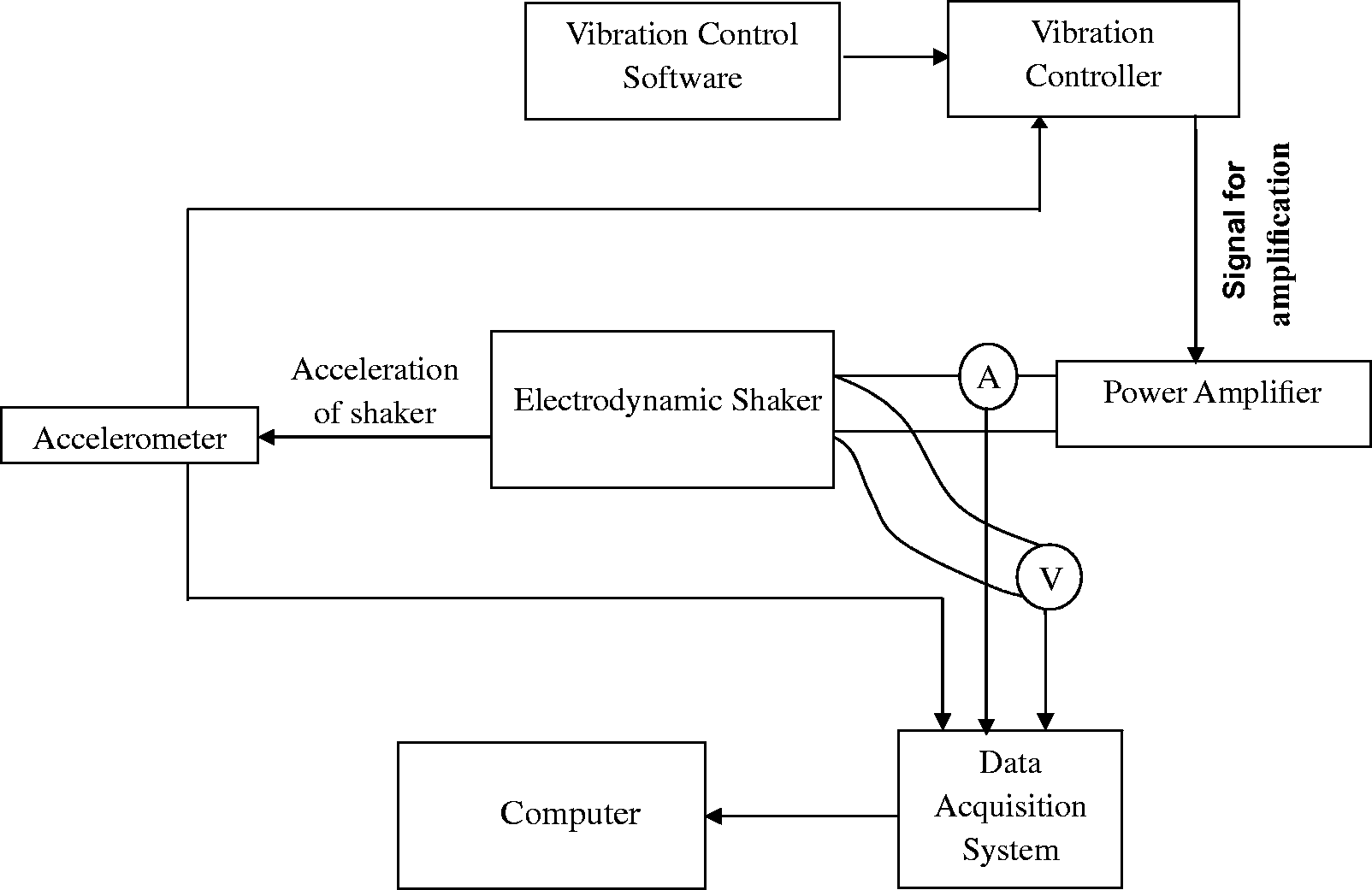

Using data from these two sets of experiments, various electro-mechanical dynamical parameters of the shaker were calculated. FFT analysis of voltage, current and acceleration signals were carried out using MATLAB and from these results, impedance versus frequency plots were obtained for unloaded and loaded conditions. We used these data to calculate the values of various model parameters as shown in Figure 3(c).

Results

Determination of model parameters

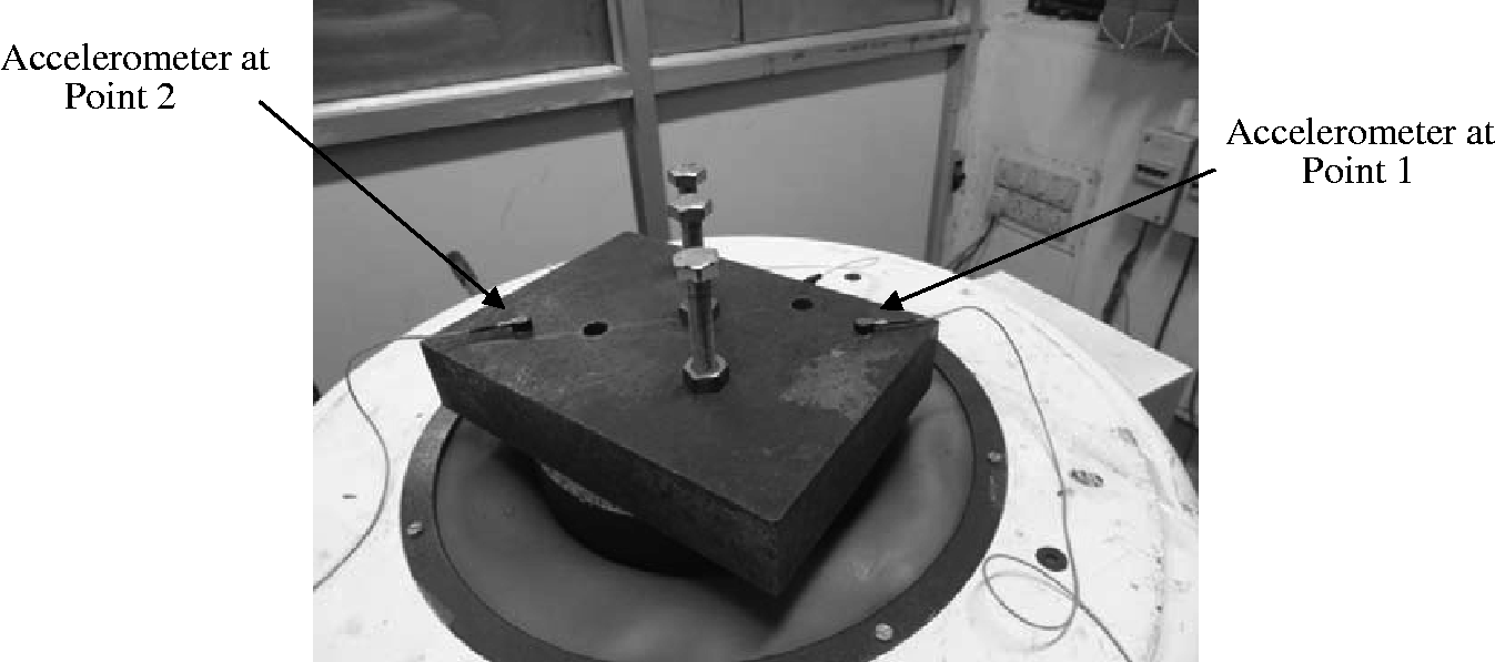
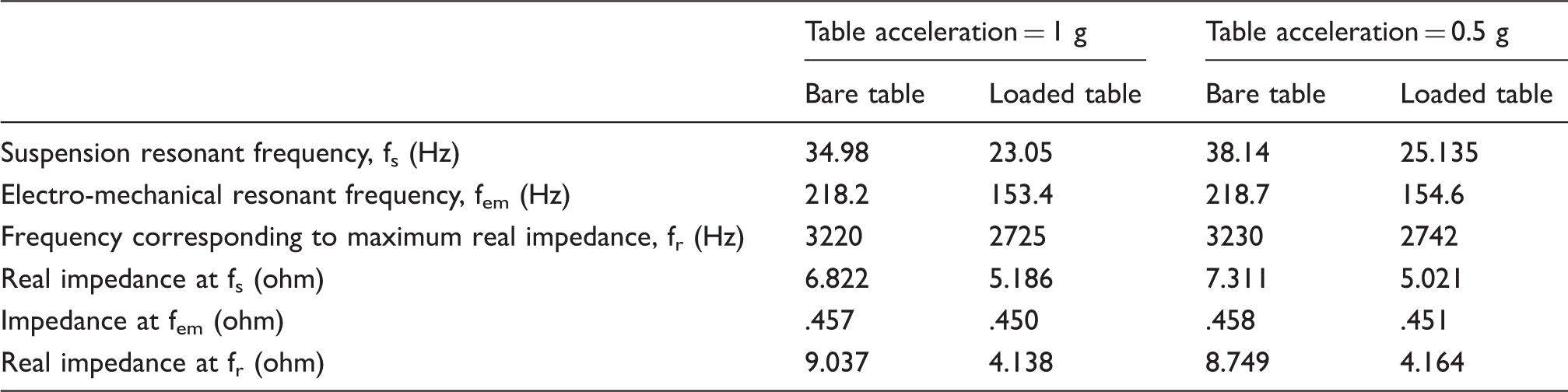
Figure 6 shows the impedance-frequency response for an unloaded and loaded shaker respectively. The first peak in Figure 6(a) corresponds to suspension resonance for an unloaded shaker excited at 1 g level. The value of this resonance is found to be 35.0 Hz. With the addition of 8.5 kg weight to the table, this frequency shifts downwards to 23.0 Hz as seen in Figure 6(b). We also note that while the absolute value of impedance peaks at suspension resonance frequency, the imaginary portion of impedance becomes zero. This is consistent with our mathematical model. We further note that imaginary part of the impedance also becomes zero at the electro-mechanical resonance. The value of electromechanical resonance for the shaker excited at 1 g level was found to be 218.2 Hz and 153.4 Hz for unloaded and loaded configurations respectively. Finally, we note that the second peak in Figure 6(a) corresponds to the armature resonance. The value of this resonance is found to be 3220 Hz for the unloaded shaker excited at 1 g level. Figure 6(b) shows that with the addition of 8.5 kg weight on the table, the frequency response curve for impedance changes in the 2000–3000 Hz region and we have three peaks instead of one in this bandwidth. Figure 8(a) gives a detailed view of these three peaks. These three peaks exist because the payload is not an ideal point mass and has its own resonance modes and its first two resonance frequencies happen to be close to the loaded shaker armature resonance frequency. To identify these frequencies of the payload, two accelerometers located at Points 1 and 2 were used. This is shown in Figure 7. Figure 8(b) and (c) are plots of acceleration, normalized with respect to voltage at Points 1 and 2, respectively.

Figure 6.

Impedance plot for the shaker at acceleration level of 1 g (a) Bare table (b) Loaded table.

Figure 7.

Accelerometer at points 1 and 2 mounted at the opposite corners of the load.

Figure 8.

(a) Detailed view of the impedance plot for the loaded condition at 1 g acceleration level. (b) Normalized acceleration responses for the Point 1 and Point 2 and the phase difference.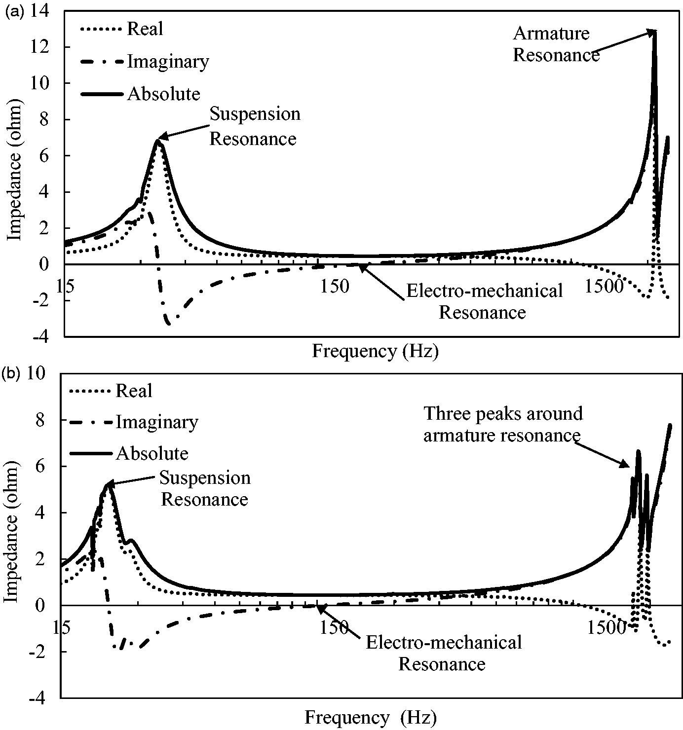

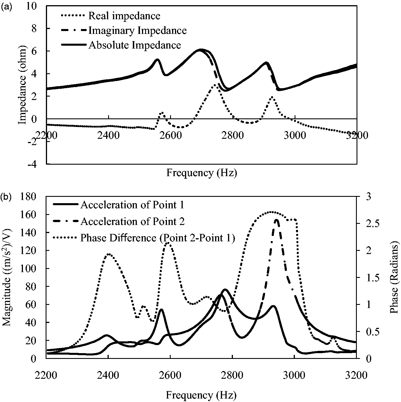
It is seen in Figure 8(a) that impedance peaks in three frequency bands. The first peak appears in the 2400–2600 Hz band, the second peak appears in the 2600–2800 Hz band and the third peak appears in the 2800–3000 Hz band.

In Figure 8(b), it can be seen that there are two frequencies for which both the accelerometers show a peak in the response, one in the range of 2600–2800 Hz and the other in 2800–3000 Hz. For the peak in the band of 2800–3000 Hz, the phase difference between the acceleration of Point 1 and Point 2 is close to 180°,i.e. the points are moving out of phase. Such a motion is akin to a seesaw motion of plate along the line passing through the centres of three bolts which hold the plate to the shaker table.

In the 2400–2600 Hz band, the value of normalized acceleration magnitude for Point 1 approaches 20 (m/s²)/V, while that for Point 2, approaches at 55 (m/s²)/V. Further, no clear peak is observed for Point 1, while the resonance of plate is evident from the peak at 2570 Hz as seen in Figure 8(b).

For the peak in the range of 2600–2800 Hz, the phase difference between acceleration of points is small and thus the acceleration of both points is somewhat in-phase, which implies the load is vibrating as a single rigid mass. Thus, a resonance frequency in this band is indicative of a shift in armature’s resonance frequency.

From such an interpretation of data, we were able to identify several important parameters of the system. Table 1 gives a summary of these special parameters corresponding to two different acceleration levels, 1 g and 0.5 g.

Table 1.

Information inferred from impedance versus frequency plots.

	Table acceleration = 1 g		Table acceleration = 0.5 g
	Bare table	Loaded table	Bare table	Loaded table
Suspension resonant frequency, fs (Hz)	34.98	23.05	38.14	25.135
Electro-mechanical resonant frequency, fem (Hz)	218.2	153.4	218.7	154.6
Frequency corresponding to maximum real impedance, fr (Hz)	3220	2725	3230	2742
Real impedance at fs (ohm)	6.822	5.186	7.311	5.021
Impedance at fem (ohm)	.457	.450	.458	.451
Real impedance at fr (ohm)	9.037	4.138	8.749	4.164

Using data in Table 1, the various model parameters were calculated for the shaker. The values of these parameters are presented in Table 2.

Table 2.

Parameters of electrodynamic shaker’s lumped model.

Symbol	Parameter	Unit	Value from 1 g data	Value from 0.5 g data
M ms	Mass of armature assembly	kg	6.52	6.52
M T	Mass of table	kg	3.84	3.87
M C	Mass of coil	kg	2.69	2.65
C ms	Suspension compliance	m/N	3.17 × 10−6	2.67 × 10−6
C C	Coil compliance	m/N	1.55 × 10−9	1.54 × 10−9
Bl	Force factor	N/A	36.53	36.54
R ms	Suspension responsiveness	(m/s)/N	4.76 × 10−3	5.13 × 10−-3
R C	Coil responsiveness	(m/s)/N	5.49 × 10−2	4.08 × 10−2
R E	Electrical resistance of coil	Ω	0.46	0.46
L E	Inductance of coil	µH	111.7	111.7

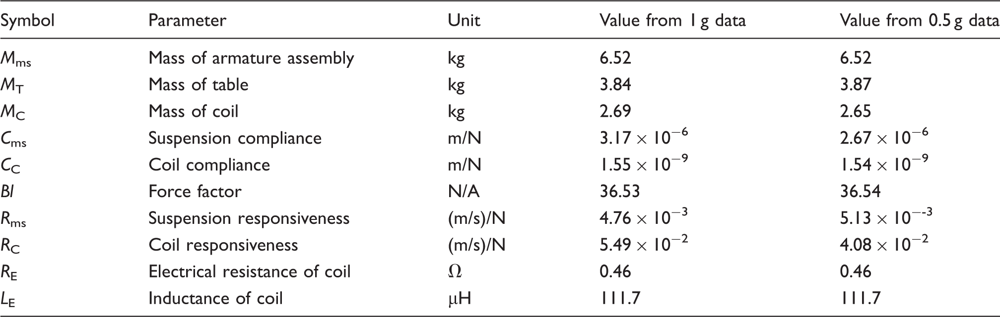
It is seen from Table 2, that the estimate of most of the model parameters based on 0.5 g and 1 g is mutually consistent. However, such a consistency is moderate for the estimates of C_ms, R_ms and R_c. This variability may be attributable to more heating at higher loads, and also due to the presence of current and displacement-dependent nonlinearities in the system.

Verification of model

Next, the parameters shown in Table 2 were used in the lumped parameter model to predict the shaker’s response as shown in Figure 3(c). Based on the data from manufacturer’s literature, the values of M_b, C_b, and R_b were estimated to be 300 kg, 1.82 × 10^-6 m/N and 0.008 (m/s)/N, respectively. To ensure that any inaccuracies in our estimates of these parameters do not materially affect the shaker’s performance, we conducted appropriate sensitivity studies. The results of these studies are reported in this work later. The model was simulated in OrCAD Capture. From simulation, various response plots were obtained and compared with experimental data to validate the accuracy of our model. In this exercise, three sets of simulations were conducted. The first set involved comparison of experimental data with predictions, when the shaker was excited at fixed acceleration levels. The second set of simulations involved conduction of sensitivity studies to evaluate the influence of M_b, C_b, and R_b on shaker response. The third set of simulations was conducted to assess the robustness of our model when the shaker was loaded with an additional mass.

Figure 9.

Transfer function for the shaker (a) 0.5 g excitation level (b) 1 g excitation level (c) 3 g excitation level.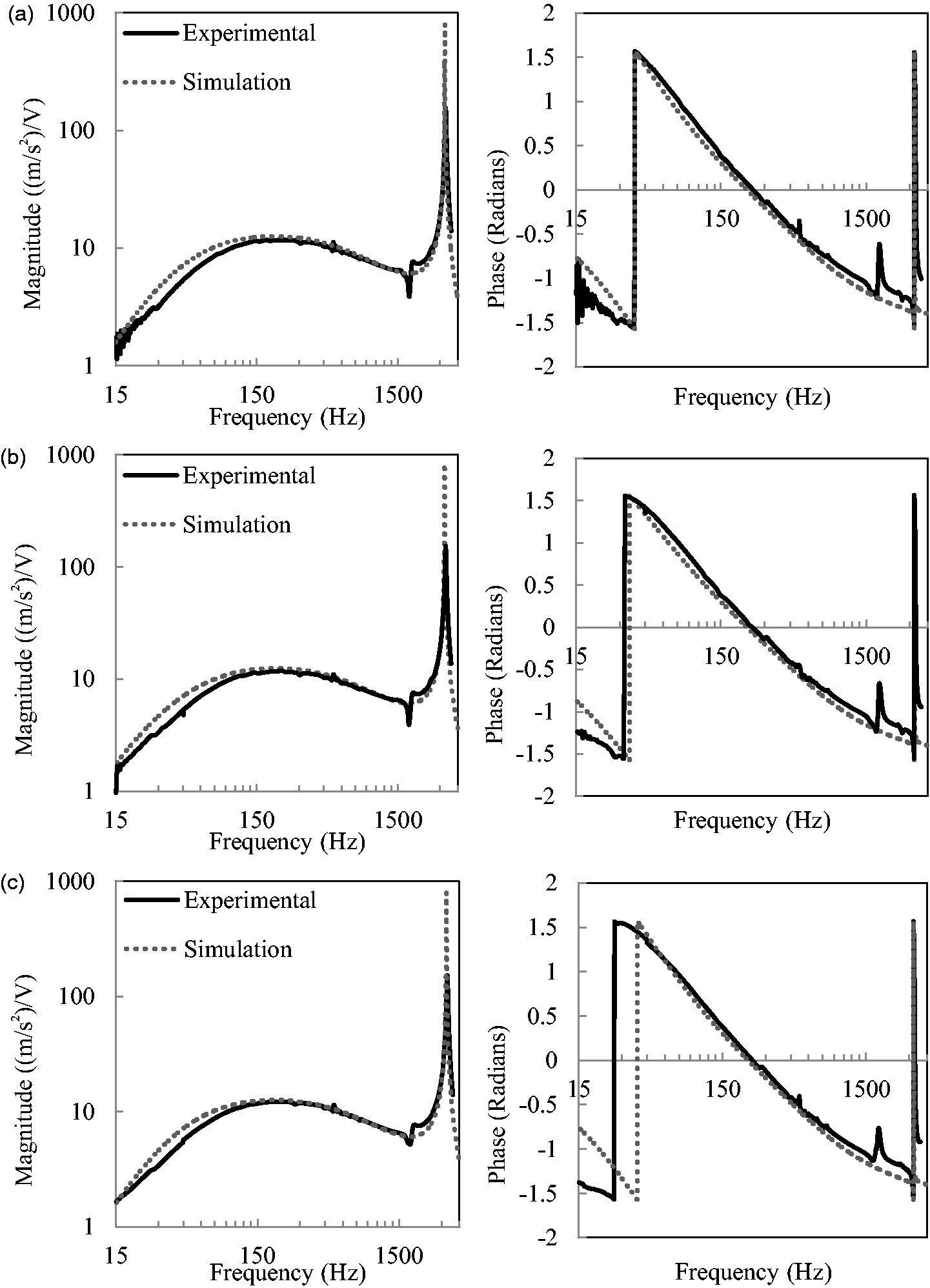

Comparison of measured and predicted acceleration response of shaker

Figure 9 shows comparisons of simulated and experimental data for shaker excited at different frequencies, at acceleration levels of 0.5 g, 1 g and 3 g. We make the following observations from the figure:

There is good agreement between simulation results and experimental data for the magnitude as well as phase plots for shaker’s transfer function.

The model also behaves well in predicting shaker response at suspension resonance particularly at 0.5 g level.

However, when the shaker is accelerated at 1 g and 3 g, there is some variation between the simulated and measured results at frequencies close to the suspension resonance. While the agreement at this resonance point is good at 0.5 g level, the predicted response gets shifted rightwards by a few Hz, vis-à-vis experimental data.

Two additional peaks are observed in the phase plot in the bandwidth of 300–3000 Hz. These peaks are possibly due to the excitation of some structural modes in the system.

Sensitivity studies to evaluate the influence of M_b, C_b, and R_b on shaker’s performance

To ensure that any inaccuracies in our estimates of M_b, C_b and R_b do not materially affect shaker’s performance in its operating bandwidth, and three sensitivity studies were conducted. In the first study, the mass of shaker body was altered significantly and the response of shaker was computed. In the second and third studies, similar simulations were conducted by varying shaker’s body isolation stiffness and its damping. In each of these three different sensitivity studies, the appropriate sensitivity parameter was assigned to three significantly different values, and the overall transfer function of the shaker was computed over a bandwidth of 1–4000 Hz. It was observed that variations in the values of the mass of body of shaker, M_b, compliance of isolation system, C_b and mechanical responsiveness of isolation system, R_b, influence shaker’s response only in the small region around isolation resonance which is out of operating range of shaker table. This justifies the use of approximate values of these parameters in equivalent electrical model of shaker which is used for simulation. Figure 10 shows the plots of transfer functions corresponding to sensitivity studies involving variations in parameters M_b, C_b and R_b, respectively.

Figure 10.

Transfer function of the shaker for different values of (a) Shaker body mass (b) Compliance of isolation system (c) Responsiveness of isolation system.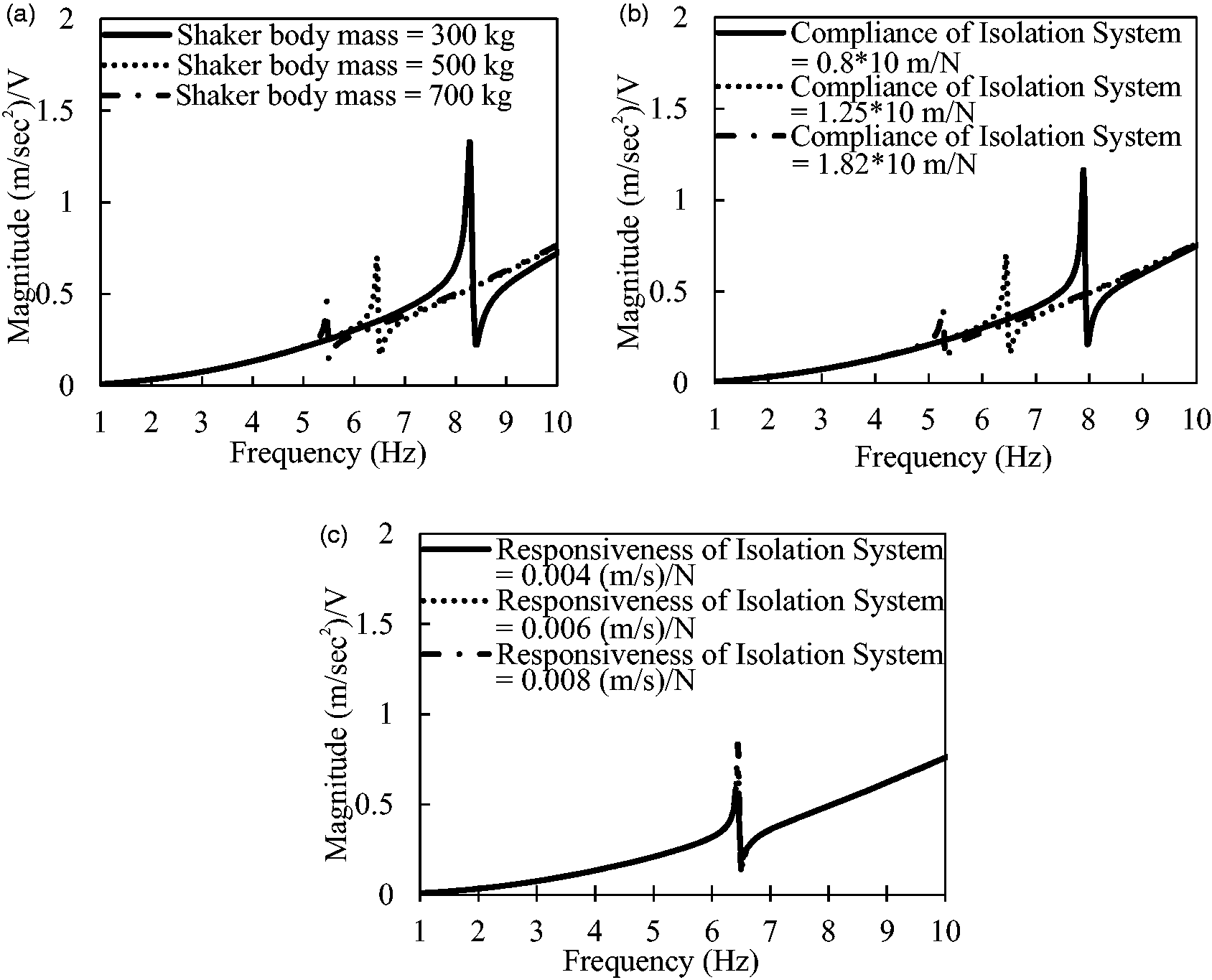

Influence of additional load on shaker’s response

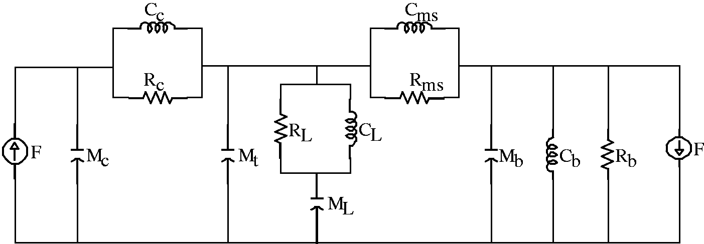
To study the influence of additional elements on the shaker’s response, an additional mass of 8.3 kg was mounted to the shaker table using four bolts as shown in Figure 11. The addition of this mass introduces three new elements, M_L, C_L and R_L in the overall system. Thus, the electrically equivalent model of the mechanical part of the shaker changes from the one shown in Figure 3(b) to the one in Figure 12.

Figure 11.

Load mounted on shaker using bolts.

Figure 12.

Equivalent mechanical circuit after addition of load.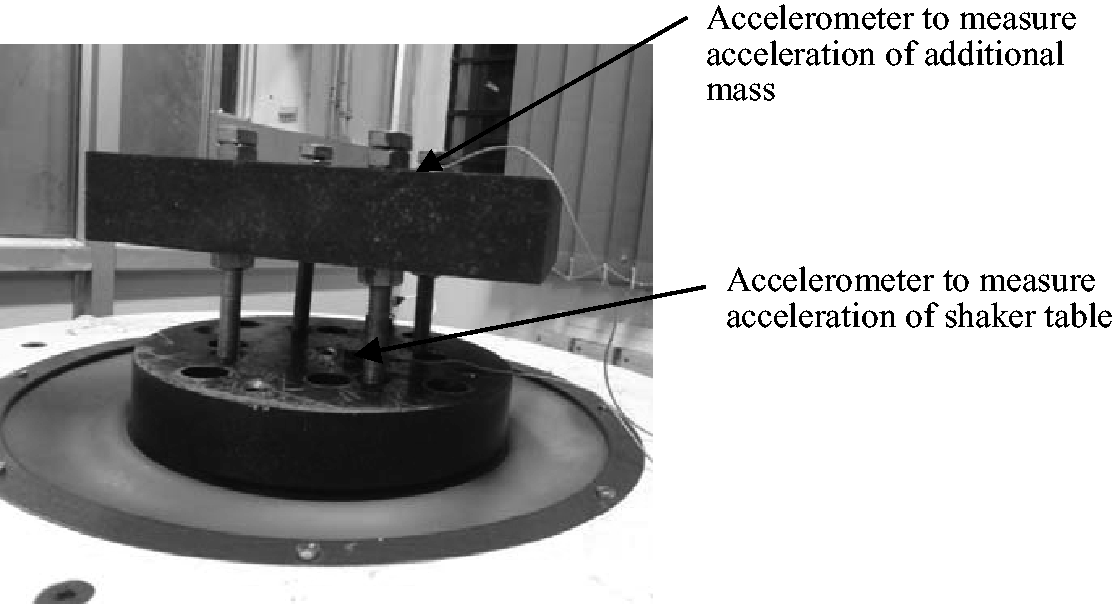

The value of C_L was computed by calculating the total compliance of four steel bolts which act as four springs in parallel. Each of these bolts had a root diameter of 8.29 mm. Further, the distance for each bolt between shaker’s head expander and upper nut was 10 cm. Using these data, the value of C_L was calculated as 2.316 × 10⁻⁹ m/N. The value of M_L is taken as 8.3 kg neglecting the mass of bolts.

To find out the value of R_L, equivalent electrical model of electrodynamic shaker was simulated for the different values of R_L and impedance versus frequency plots were obtained. The value of R_L for which impedance plot obtained from simulation matched with experimental data was chosen as value of R_L. This value was found to be .0021 (m/s)/N.

After fitting the values of M_L, C_L and R_L in equivalent electrical model of shaker, response of shaker table and response of the load was predicted and compared to experimental data. The experimental data correspond to a shaker loaded with additional weight as shown in Figure 11, and excited at 1 g.

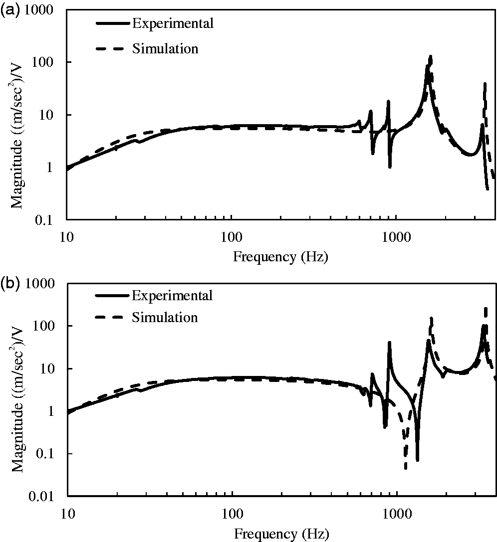
Figure 13 shows comparison of the predicted response of additional mass and shaker table with the experimentally measured response. The following observations can be made from the figure:

The predicted and measured acceleration response curves agree very well for the bandwidth of 10 to 900 Hz.

A resonance peak near 1500 Hz is observed in the predicted response of shaker table as well as that for the load from Figure 13. This is consistent with the experimental data.

Predicted response curve of table of shaker shows an anti-resonance point at 1130 Hz. This frequency is close to experimentally observed anti-resonance point at 1340 Hz as seen in Figure 13(b). The appearance of anti-resonance in the response curve of table of the shaker shows that response of table of shaker is influenced by the characteristics of load mounted on it.

Experimentally obtained plots of magnitude of acceleration normalized with respect to voltage versus frequency show four resonant peaks excluding suspension resonance and armature resonances, while predicted response has only one additional resonant peak. This difference between predicted and measured responses is possibly attributable to the presence of other modes in loaded structure, which include bending modes. Please note that these resonances are primarily due to the presence of mounting bolts and are different than those for the plate which is shown in Figure 8 and discussed in this Section. These additional degrees of freedom are not captured in our lumped parameter model and can be accounted for by having additional degrees of freedom in the model.

Figure 13.

Magnitude of normalized acceleration (a) additional mass (b) loaded table.

Conclusion

In this article, an equivalent electrical model of medium sized electrodynamic shaker has been developed. Experiments have been conducted to obtain impedance versus frequency and normalized acceleration versus frequency for bare table and also for a loaded table. Equivalent electrical model of medium sized electrodynamic shaker has been analysed. Based on the analysis of equivalent electrical model and experimentally obtained data, key linear electrical and mechanical parameters of medium sized electrodynamic shaker have been determined.

Further, these parameters for an electrodynamic shaker have been used to predict the acceleration response of the shaker. From such a simulation, impedance versus frequency and normalized acceleration versus frequency have been obtained. These plots were subsequently compared with corresponding experimental data. Their comparison shows that lumped parameter model of medium sized electrodynamic shaker is reasonably accurate. However, the deviation between experimental data and simulation results becomes noteworthy near armature resonance. Such a deviation is attributable to the errors in the estimation of electrical resistance due to the skin effects and role of air damping.

The sensitivity of shaker response to presence of additional payload has also been investigated. Here, the load was mounted on the shaker table in such a way that it resembles a spring-mass-damper system of single degree of freedom. Using modified equivalent electrical model, the response of shaker table and the response of load has been predicted. Predicted and actual responses of the shaker are reasonably similar, thereby validating the proposed equivalent electrical model of the electrodynamic shaker. It is also observed from the actual response of the shaker table as well as from its predicted response that response curve of shaker table is influenced by characteristics of the load mounted on it.

In this article, linear electrical and mechanical parameters of a medium sized electrodynamic shaker are determined. Such an approach works well for low values of excitation voltages. For high excitation voltage levels, the electrodynamic shaker behaves non-linearly. Major non-linear parameters are transduction constant, Bl, armature suspension compliance, C_ms, and inductance of armature coil, L_E. Further analysis and experiments can be done to understand the non-linear behaviour of the large electrodynamic shaker.