
Abstract
Experiences of past earthquakes demonstrate that pipeline systems have no proper performance when exposed to severe earthquakes. In this study, sensor and damper placement approaches are presented for doing reliable health monitoring and seismic retrofitting of the piping networks. Since most of the available sensor placement methods are based on modal analysis results, the authors propose a new scheme that relies on the nonlinearity which utilizes nonlinear time history analysis results, and genetic algorithm is selected to act as the methodology of optimization as well. The results demonstrate that the proposed optimal sensor configuration strategy is more accurate and efficient than the extended modal assurance criterion method. To assess the number of sensors, a sensitivity analysis is undertaken in which the number of sensors computed optimally by the proposed algorithm contains the least convergence error. In addition, the number of iterations and the time consumed in the proposed approach are considerably less than the extended modal assurance criterion method. Moreover, the efficiency of the proposed sensor placement scheme was compared with a new algorithm proposed by Sun and Büyüköztürk, named discrete artificial bee colony, where the simulation result demonstrates high accuracy of the proposed sensor configuration approach. The initial time history analysis results show the vulnerable points of the system, which destroyed due to the applied seismic waves. Hence, to enhance the seismic performance of the system, piezoelectric friction dampers are optimally placed, where it can be clearly seen that the optimal arrangement of piezoelectric friction dampers in the piping system can significantly decrease the seismic response.
Keywords
Introduction
Real-time and continuous inspection of damage to piping systems after seismic events is vital for an early emergency response, efficient preparation of rescue plans, and mitigation of the disastrous consequences. Assessment is particularly challenging for buried pipelines since they are under the soil. 1 Existing technologies on the assessment of underground piping systems are mainly based on the use of instruments that can be applied in the interior of the pipeline. These tools can involve different types of smart sensors, typically depending on the kind of the pipeline. 2
Real-time pipeline monitoring systems, with wired or wireless sensors, were extensively developed and applied in the last decade. 3 Xiaohang and Hua 4 designed an underground pipeline three-dimensional (3D) information system based on the inertia technology. Hou et al. 5 studied the leakage detection of the natural gas pipeline experimentally in which they utilized fiber Bragg grating sensors.
Different approaches for sensor placement and damage identification were proposed, including the modal kinetic energy (MKE) method, 6 the effective independence (EI) method, 7 the modal assurance criterion (MAC), 8 Artificial Neural Network (ANN), 9 wavelet transform approach, 10 and the damage location vector. 11 Yao et al. 12 engaged genetic algorithm (GA) as a substitution to the EI, and the determinant of Fisher Information Matrix (FIM) was selected as a objective function. Kammer and Tinker 13 proposed a sensor configuration method containing triaxial accelerometers based on EI to carry out modal vibration tests. Ngatchou et al. 14 presented a type of improved particle swarm optimization (PSO) algorithm named sequential-PSO to layout the sensors. Ferentinos and Tsiligiridis 15 proposed a multi-objective optimization strategy to implement in the wireless sensor networks via GA. Kang et al. 16 investigated three-sensor configuration performance indexes and proposed a virus co-evolutionary partheno-genetic algorithm. Flynn and Todd 17 proposed a novel Bayesian scheme to carry out optimal sensor placement which could be applicable on active sensing as well. Chen and Nagarajaiah 18 presented a new method according to the GA to identify the detection filter-based decentralized controller in which numerical and laboratory results demonstrated that the strategy can detect structural damage. Zhou et al. 19 introduced a cluster-in-cluster firefly algorithm for the optimum sensor deployment. Yi and coworkers 20 proposed an immune monkey algorithm through composing monkey algorithm with immune algorithm to implement optimal sensor placement in Canton Tower.
Passive energy dissipation systems such as viscoelastic dampers, tuned mass dampers and friction dampers were widely utilized to decrease the dynamic response of infrastructures subjected to seismic loads. 21 Among the dissipation systems, friction dampers with various designs were expanded and exerted for the seismic protection, as their hysteretic behaviors could be kept stable for cyclic loads and desirable slip loads are easily acquired by regulating normal forces acting perpendicularly to a friction surface, as well as their simple energy dissipation mechanism and easy manufacturing, installation, and maintenance.22–26 Piezoelectric actuators are especially interesting due to their high response velocity, low energy demand, compact size, and appropriate functionality within a broadband frequency range. 27 Because of that, several scholars have studied about piezoelectric friction dampers to enhance damping in seismic isolation systems and in combination with tuned mass dampers.28–32 Ladipo and Muthalif 33 proposed the designing procedure of an active dynamic vibration absorber system by PID control technique to adaptively tune the active dynamic vibration absorber stiffness property to mitigate the vibration of a multi-mode system at modal frequencies. Also, an active vibration control approach conducted on a simply supported thin plate, which was modeled using Lagrange’s theory was proposed by Nor et al. 34 Chen and Chen 35 evaluated the performance of the semi-active control strategy and of a fabricated piezoelectric friction damper experimentally. They conducted a series of shake table tests on a quarter-scale, three-storey building model controlled by piezoelectric friction dampers. Zhao and Li 36 studied the seismic reductions of a building structure with piezoelectric friction damper and semi-active fuzzy control approach using a series of shaking table tests and numerical analyses. Kumar et al. 37 investigated the performance of pipelines subjected to seismic waves which were equipped with semi-active variable stiffness dampers. Pardo-Varela and Llera 38 studied the development of a semi-active piezoelectric friction damper for improving the seismic performance of large-scale structures.
Herein, a new optimal sensor placement method is proposed which utilizes nonlinear time history analysis results, unlike other methods which use modal analysis results, to locate the position of sensors more precisely leading to explore the structural deficiencies before a severe seismic event. In addition, to mitigate the seismic damages imposed to the piping system, an efficient type of dampers (piezoelectric friction dampers) is engaged where those devices are installed optimally to decrease the seismic response of the system considerably. In this study, optimal placement of sensors and piezoelectric friction dampers is undertaken using dynamic analysis results in which the water pipeline network of a district is taken into account for finite element modeling. The soil–pipe interaction is modeled through nonlinear Winkler Foundation model in which the Numerical modelling section represents the soil–pipe interaction. The remainder of the paper is arranged as follows: section “Dynamic analysis” describes the dynamic analysis procedure containing modal analysis in addition to nonlinear time history analysis using seismic records of near-fault excitations. Numerical verification of finite element model by ANN section investigates the validation of finite element model by ANN in which the finite element and ANN results are compared by a statistical test. Three sensor placement strategies are presented in optimal sensor placement section, in which the authors’ proposed algorithm depends on the nonlinearity and utilizes nonlinear time history analysis results in which GA is also employed to act as the methodology of optimization. Then the force-control theory and optimal placement of piezoelectric friction dampers are presented. Eventually, conclusions are drawn in the final section.
Soil–pipe interaction
A buried pipe and its adjacent soil elements attract earth embankment loads and live loads in accordance with a fundamental principle of structural analysis in which stiffer elements attract greater proportions of shared loads than those that are more flexible. The surrounding soil is of greater stiffness than the flexible pipe and of lesser stiffness than the rigid pipe. 39
Soil properties representative of the backfill should be used to compute axial soil spring forces. Other soil spring forces should generally be based on the native soil properties. Backfill soil properties are appropriate for computing horizontal and upward vertical soil spring forces. It is possible when the extent of pipeline movement relative to the surrounding backfill soil is not influenced by the soils outside the pipe trench.
For each soil spring, an elastic-perfectly plastic force–deformation relationship was assumed and the expressions were adopted from the ALA-ASCE guideline.
40
The maximum soil spring forces and associated relative displacements which are necessary to develop these forces are computed using the following equations. The maximum axial soil force per unit length of pipe Tu transmitted to the pipe is defined as
40

The maximum lateral soil force per unit length of pipe Pu transmitted to the pipe is defined as
40

The maximum vertical bearing soil force per unit length of pipe Qd transmitted to the pipe is also defined as
40

The soil–pipe interaction was modelled via the nonlinear Winkler Foundation model in which the interactive behaviour has been represented by nonlinear discrete soil springs. The arrangement of spring elements and distribution of their stiffness around the pipe’s circumference is of significant importance. Nonlinear force–displacement characteristics of springs per unit length of the pipe are illustrated in Figure 1.
40
As shown in Figure 1, Qu indicates the maximum vertical upward soil-bearing capacity. Also, Δ
p
, Δ
t
, Δ
qd
, and Δ
qu
are the horizontal displacement to develop Pu, axial displacement to develop Tu, vertical displacement to develop Qd, and vertical displacement to develop Qu, respectively.
Force–deformation relationship of the soil springs.
40
(a) transverse horizontal spring, (b) axial spring and (c) transverse vertical spring.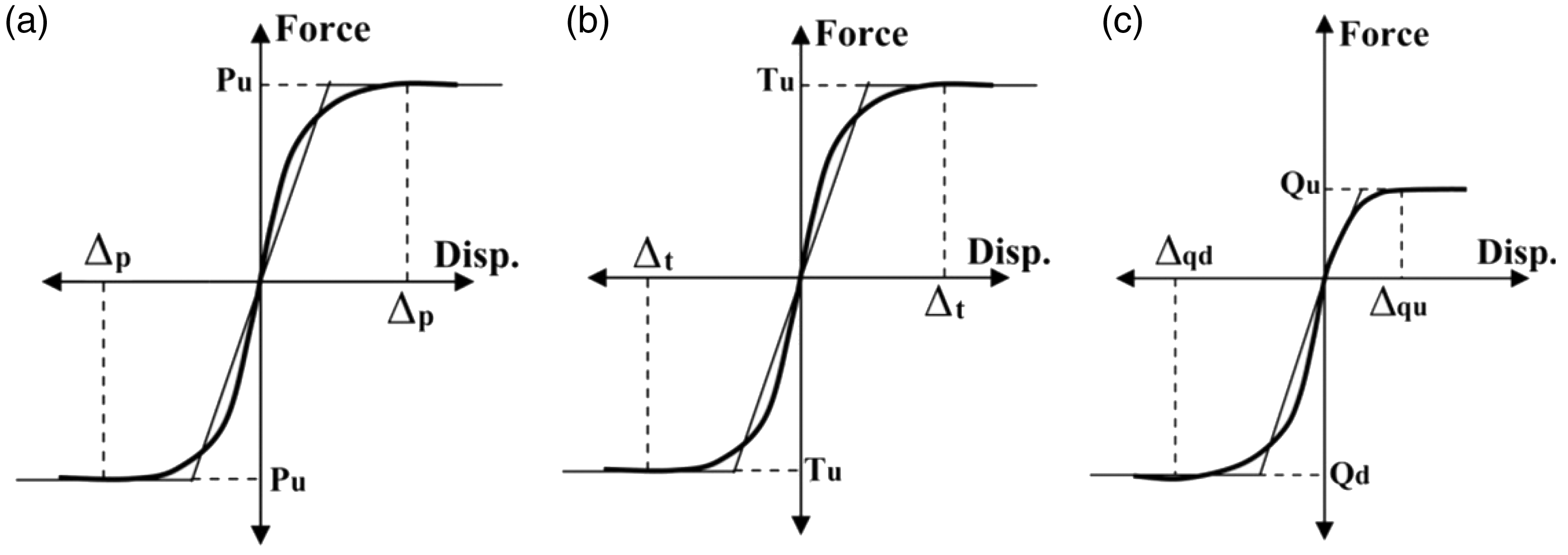
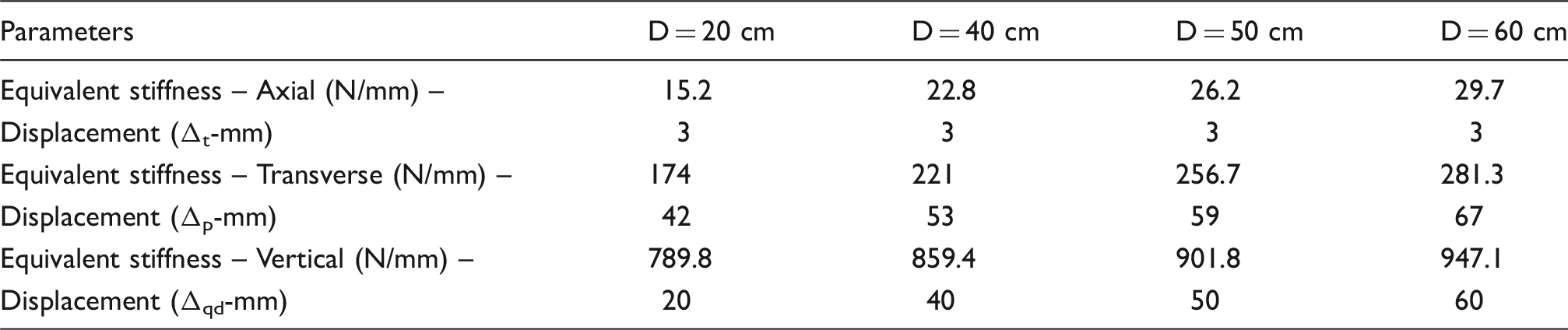
Equivalent stiffness and corresponding displacement of translational nonlinear soil springs.
Numerical modelling
A finite element program is used to model and analyse the piping system subjected to static and dynamic loads. The software provided a built-in structural analysis with shell elements to enable the mass and flexibility of structural supports as part of their piping analysis. The software calculates static and dynamic response properties of complex piping systems and structures using finite element techniques. This provides structural modeling options specified beta angles to orient beam local cross-section axes with global axes, rigid end lengths to account for the connectivity of end points to other members in the structural system, and end releases to model pinned connections.
The static capability includes the computation of piping and structural deformations, member loads, and stress caused by an arbitrary set of thermal loads, applied loads and displacements. The dynamic capabilities, on the other hand, include mode shapes and natural frequencies, response spectra, phased harmonic load analysis, time history dynamic analysis and force spectra analysis. The computational method is Argyris finite element analysis of Castigliano’s Theory of Equilibrium of Elastic Structures. Stresses are calculated in accordance with the first principles of stress analysis, the Heuber, von Mises, Hencky failure theory, and the Tresca failure theory as required by the American Society of Mechanical Engineers (ASME) piping code.
41
Figure 2 illustrates the finite element model of the water pipeline network schematically. The material properties of the pipes derived from the ASME B-31.3 code
41
are summarized in Table 2.
Finite element model of pipeline network considering soil–pipe interaction. Material properties of the studied pipeline.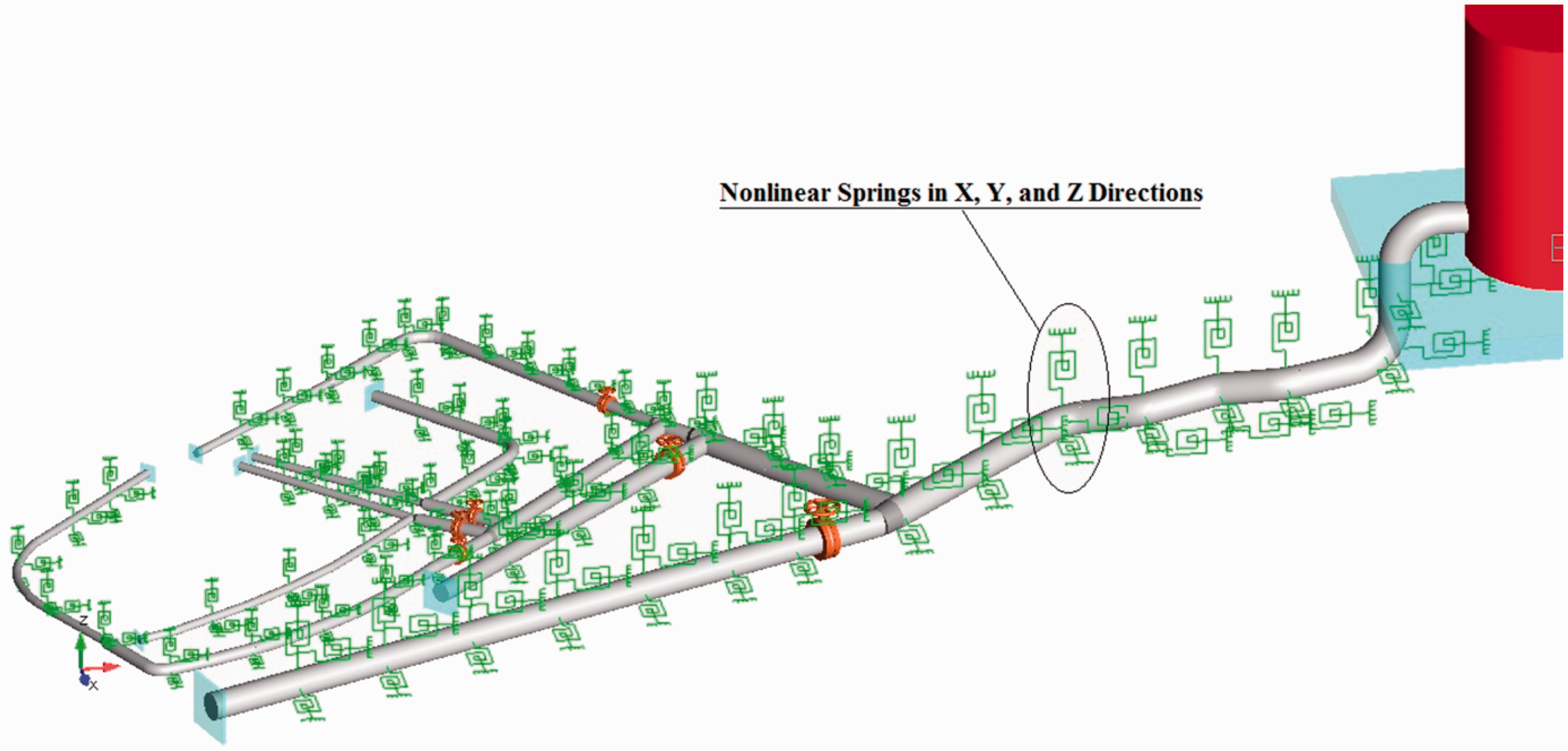

In the current study, three different types of soil conditions – dense sand (Ø = 30°), loose sand (Ø = 22.5°), and soft clay (Ø = 0°) – are taken into account as the piping system is generally buried over a long length. Two kinds of soil conditions, including sand and soft clay, are considered in this study. However, since the shear stress on the failure plane, particularly in the sand, is varied with the angle of internal friction, the sand soil condition has been divided into two types, dense and loose sand, depending on the angle of internal friction. In the present study, the dense sand is assumed to have a 30° of the angle of internal friction, while the loose sand is assumed as a 22.5° of the angle of internal friction. The rationale behind the present classification lies in the use of Mohr-Coulomb failure criterion employed as nonlinear discrete soil springs of Winkler Foundation model methodology. 40 Regarding the numerical modelling of the pipeline network, inelastic line elements have been utilized to model the pipeline. In this study, the soil surrounding the pipeline was modeled using nonlinear discrete springs in which these springs simulated the components of soil–pipe interaction in axial, transverse horizontal, and transverse vertical directions.
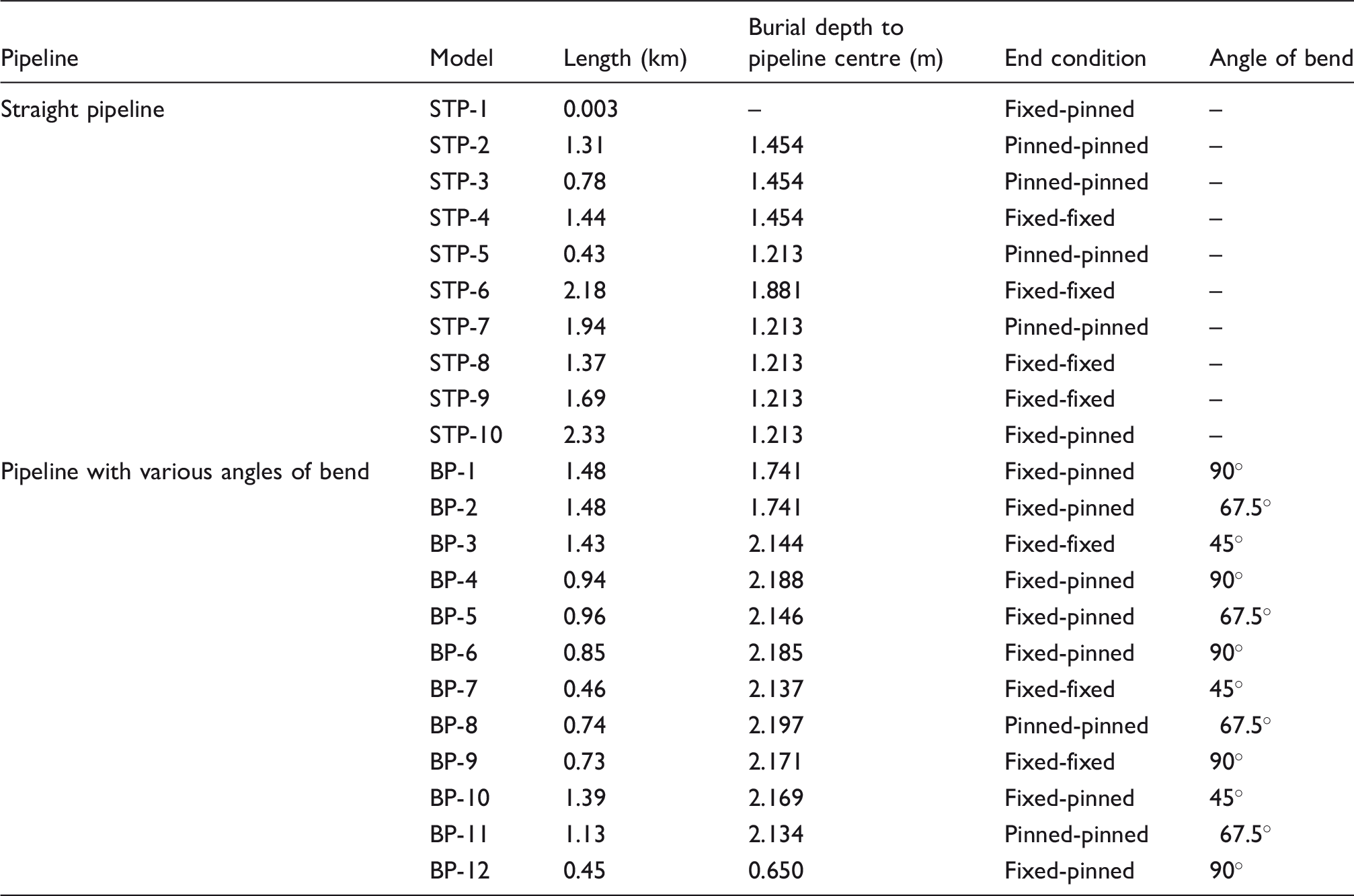
Twenty-two different pipeline segments for finite element analysis.
Dynamic analysis
Modal analysis
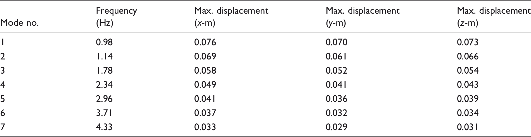
Dynamic loadings have a tendency to increase the response of the structure beyond the response obtained if the same load is applied statically. There are three mass degrees of freedom per node and the finite element software lumps the mass of the pipe, components and contents, etc. at the associated node point. This assumption yields a diagonal mass matrix with no mass coupling terms. It should be noted that rotational mass is ignored, except for points with eccentric weights in which in these points, there may be up to three additional rotational masses and thus three additional mass degrees of freedom. Figure 3 illustrates the first four mode shapes of the pipeline network. Table 4 demonstrates the first seven frequencies and maximum displacements in the presented modes in x, y, and z-directions.
The first four mode shapes of the water pipeline network. Values of frequency and maximum modal displacements of the piping network.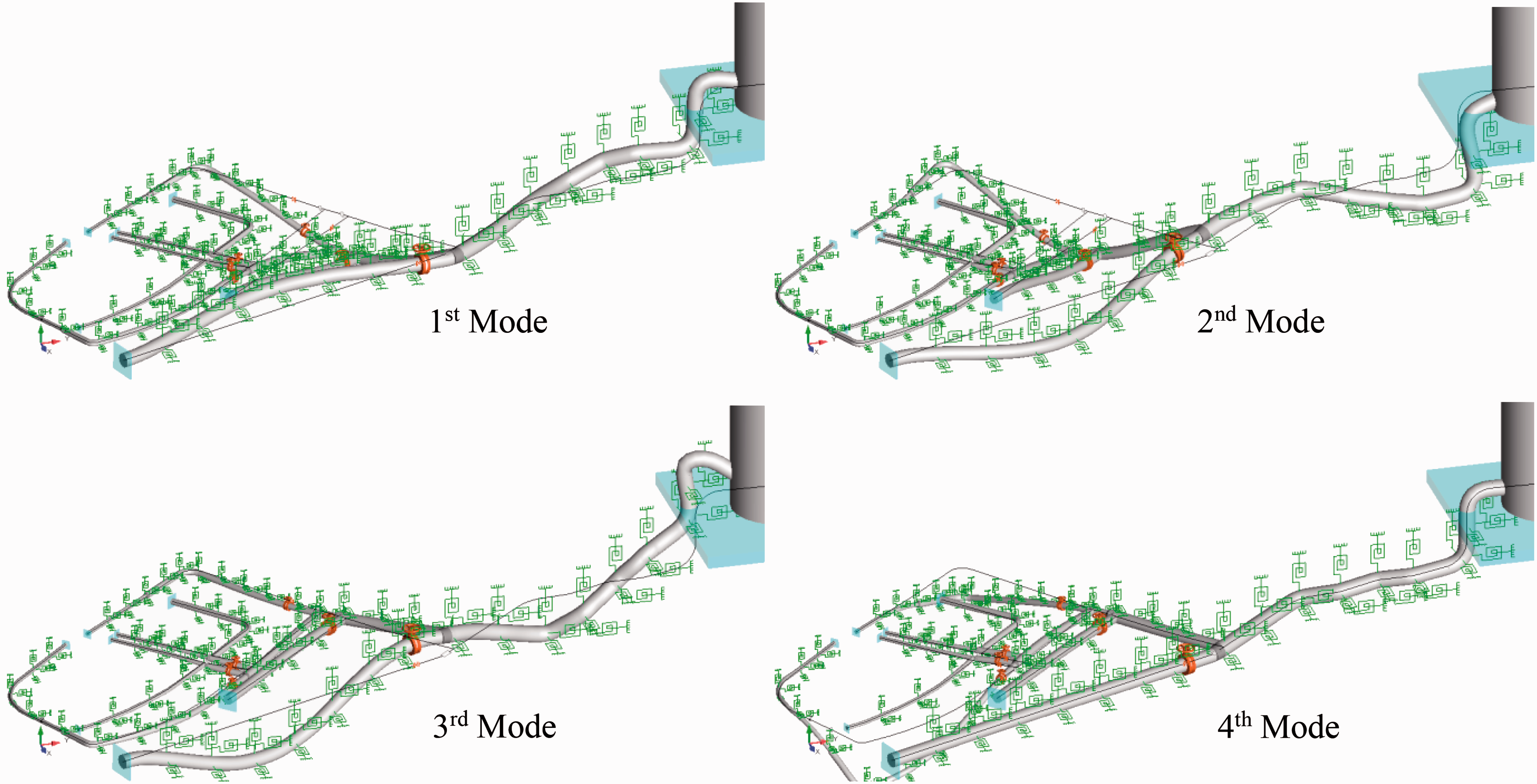
Nonlinear time history analysis
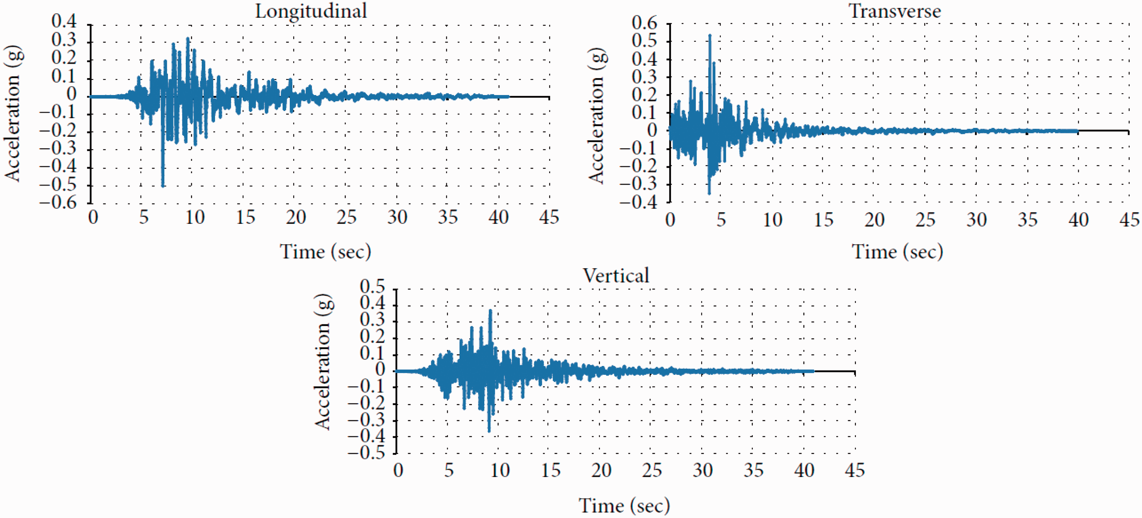
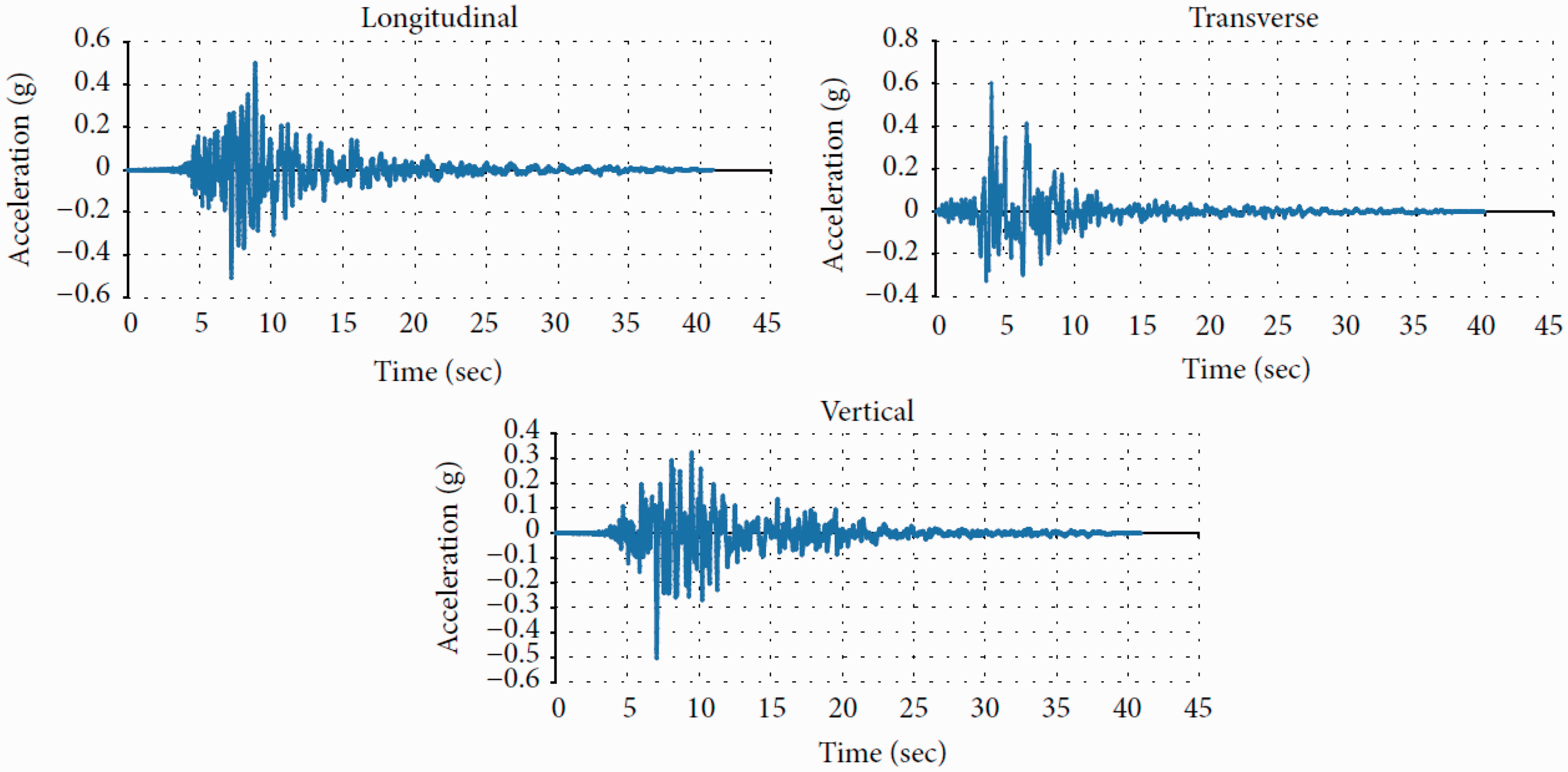
The seismic ground motions utilized in the following nonlinear time history analyses are the accelerograms recorded at CHY046 station in Taiwan during the 1999 Chi-Chi earthquake, Fukushima station in Japan during the 1995 Kobe earthquake, and Barstow station in the United States during the 1992 Landers earthquake. These seismic records were chosen from Pacific Earthquake Engineering Research (PEER) strong motion database for the purpose of dynamic analysis.
42
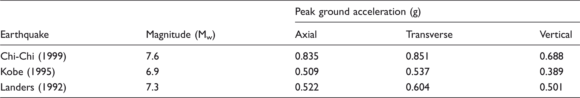
Longitudinal, vertical, and transverse components are applied in time history analyses, and acceleration time histories of the ground motion components are illustrated in Figures 4 to 6. Table 5 also presents the parameters of the selected earthquake ground motion records.
Acceleration time histories of the 1999 Chi-Chi earthquake. Acceleration time histories of the 1995 Kobe earthquake. Acceleration time histories of the 1992 Landers earthquake. Characteristics of earthquake ground motions.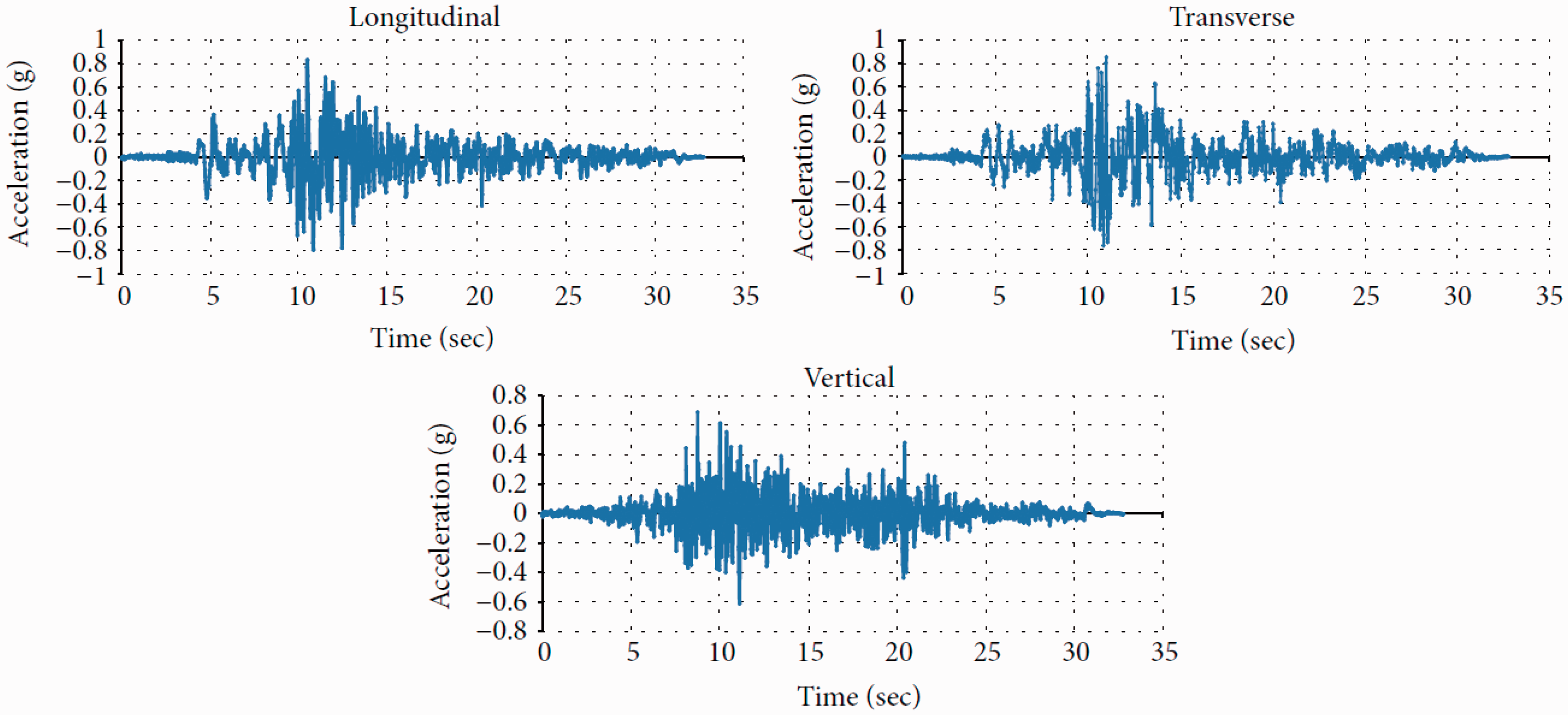
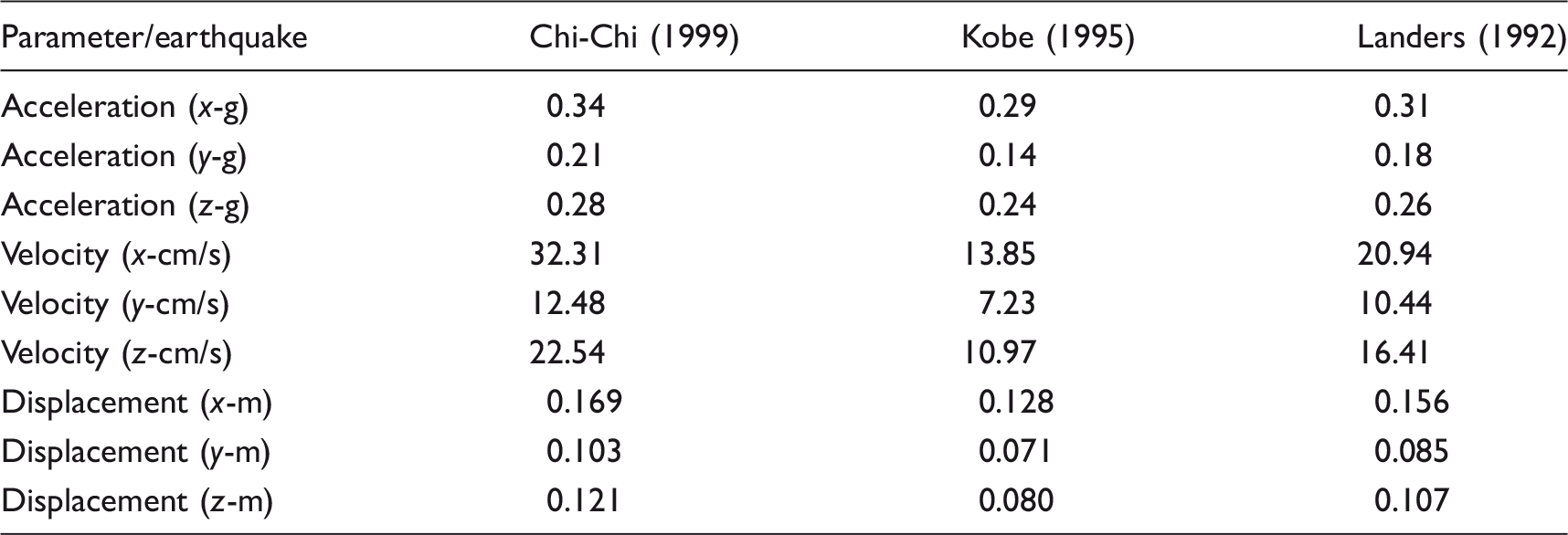
Maximum values of acceleration, velocity, and displacement time histories at node 46 in x-, y-, and z-directions.
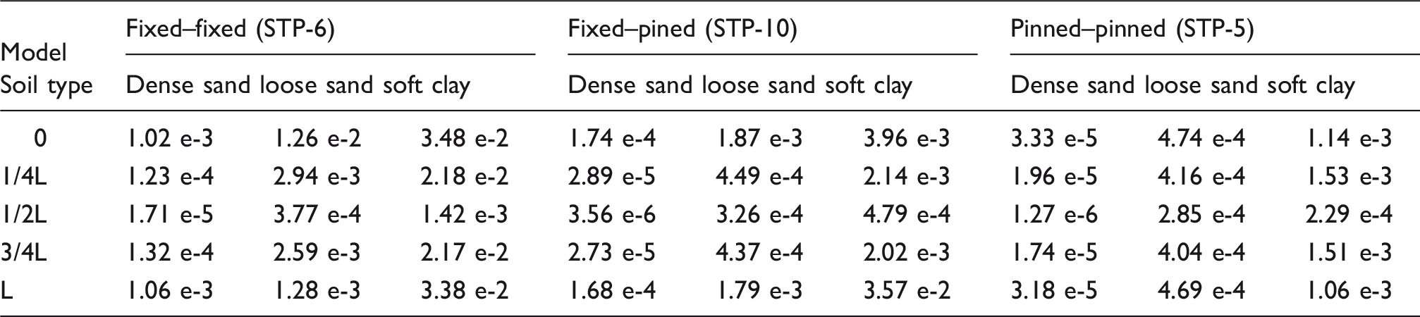
Maximum values of strain under different restraints and soil types subjected to the 1999 Chi-Chi earthquake.
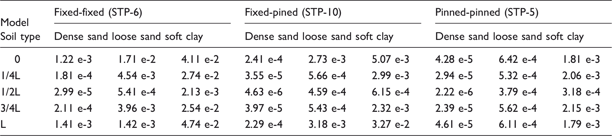
L: the pipeline length.
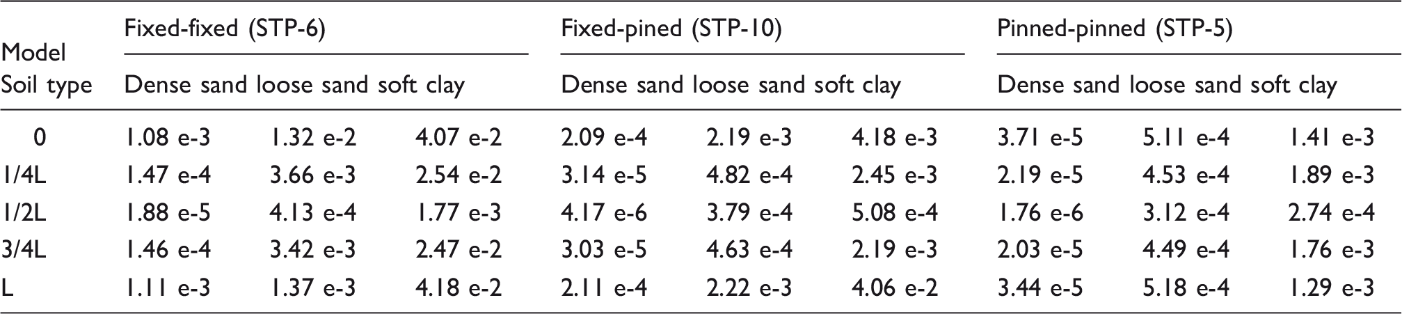
Maximum values of strain under three different restraints and soil types subjected to the 1995 Kobe earthquake.
L: the pipeline length.
Maximum values of strain under three different restraints and soil types subjected to the 1992 Landers earthquake.
L: the pipeline length.
Numerical verification of finite element model by ANN
In this study, an attempt has been done to train a neural network in order to validate the numerical results by comparing the finite element and ANN results through a statistical test. The network is used with two layers consisting of the Tansig and Purelin functions in the first and second layers, respectively. After normalization process of all data, 20% of them were considered as testing data. The remaining 80% data were divided into two groups of validation and training data, while 20% of them were validation and the others were training data.
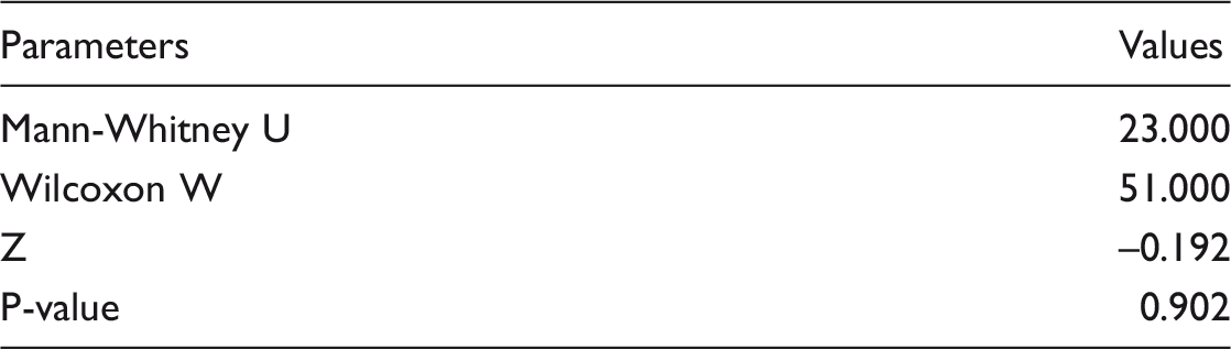
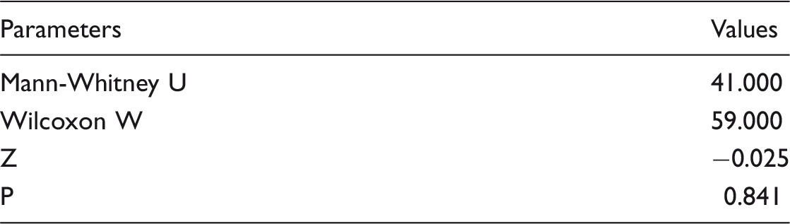
Totally, there were 1120 series of data containing 224 testing, 179 validation, and 717 training datasets. These are entire data used to develop the ANN model. Figure 7 shows the regression of the presented ANN. In addition, Mann-Whitney test was used to compare the trained and numerical data. The Mann-Whitney test is engaged to examine whether two independent samples of observations are drawn from the same distributions. As a benefit of this examination, two samples under consideration cannot essentially have the identical number of observations. The mentioned test, which also named the Wilcoxon rank sum test, is a nonparametric test comparing two unpaired groups. For the Mann-Whitney test, the null hypothesis would be a little difficult to perceive. The null hypothesis is that the distributions of both groups are identical, so that there is a 50% probability, which an observation from a value randomly chosen from one population exceeds an observation randomly chosen from the other population. The results of the Mann-Whitney test are presented in Table 10. This table is a test statistics table and shows the actual importance value of the test. The P-value is the level of marginal significance within a statistical hypothesis test, representing the probability of the occurrence of a given event. As seen, based on the obtained P-value, there is good conformity between the ANN and finite element results.
Regression of the presented ANN. The results of Mann-Whitney test for comparison between finite element and ANN results.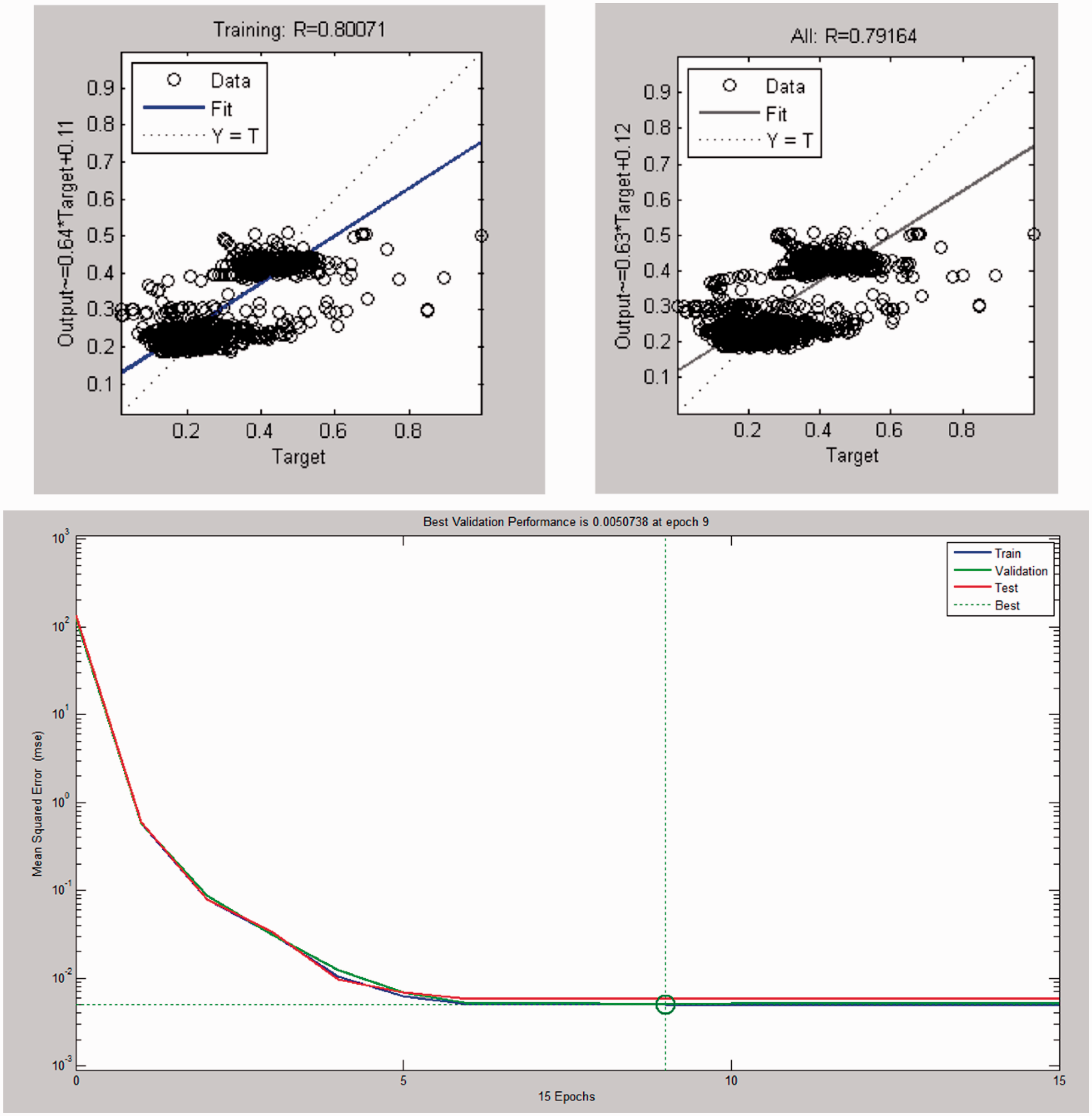
Optimal sensor placement
Sensor placement scheme based on nonlinear dynamic analysis
Numerous strategies were presented for optimal sensor placement and pipeline health monitoring which were extensively reported in the literature. Some methods were advanced through a number of methodologies and criteria, some are based on intuitive placement or heuristic approaches, yet others employ systematic optimization methods. In this section, a novel optimal sensor placement method is proposed that utilizes nonlinear time history analysis results.
The structural systems can behave nonlinearly because of the nonlinear performance of some components within the systems. For nonlinear systems, the classical frequency response function (FRF) cannot acquire a comprehensive description for the system dynamical characteristics. Hence, the modal analysis results could not be engaged as exact inputs to perform an accurate optimal sensor configuration.
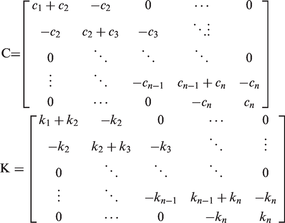
If all springs and damping have linear behavior, the system is a multi-degree-of-freedom (MDOF) linear system, and the governing motion equation can be presented as

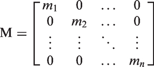
Equation (5) is the basis of the modal analysis method, which is a strong technique for indicating dynamical properties of engineering structures.
43
In the linear system, the displacements 
Supposing that 
Denote


Then, the motion of the MDOF system can be obtained by

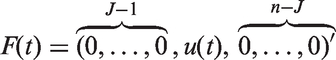
Equations (7) to (10) are the motion governing equations of nonlinear MDOF systems with multiple nonlinear components. The 
When a system is linear, its dynamic characteristics can be simply analyzed using the FRFs defined as the Fourier transform of 


In this study, Roulette Wheel Selection (RWS) approach is employed. The RWS is a mechanism to probabilistically choose individuals according to some measure of their performance. The basic operator for producing new chromosomes in the GA is that of crossover. The crossover is the operator that generates new individuals (offspring) by exchanging bits of some randomly selected individuals (parents). In GAs, mutation is randomly applied with low probability, typically in the range 0.001 and 0.01, and modifies elements in the chromosomes.
48
The size of the searching space includes the number of nodes on the finite element model excluding constrained and vibration nodes of the chosen modes. Although the piping network has a large number of degrees of freedom, just translational degrees of freedom p are taken into account for possible sensor configuration procedure as rotational degrees of freedom are normally difficult to measure. Hence, 54 translational degrees of freedom are considered for sensor installation. In the sensor placement approach, 14 accelerators are considered to be installed in the presented system. Figure 8 illustrates the flowchart of the proposed sensor placement strategy. In the flowchart, Axi, Ayi and Azi represent the maximum acceleration values of the system, which computed through nonlinear dynamic analysis, in x-, y-, and z-directions, respectively.
Flowchart of the proposed sensor placement strategy.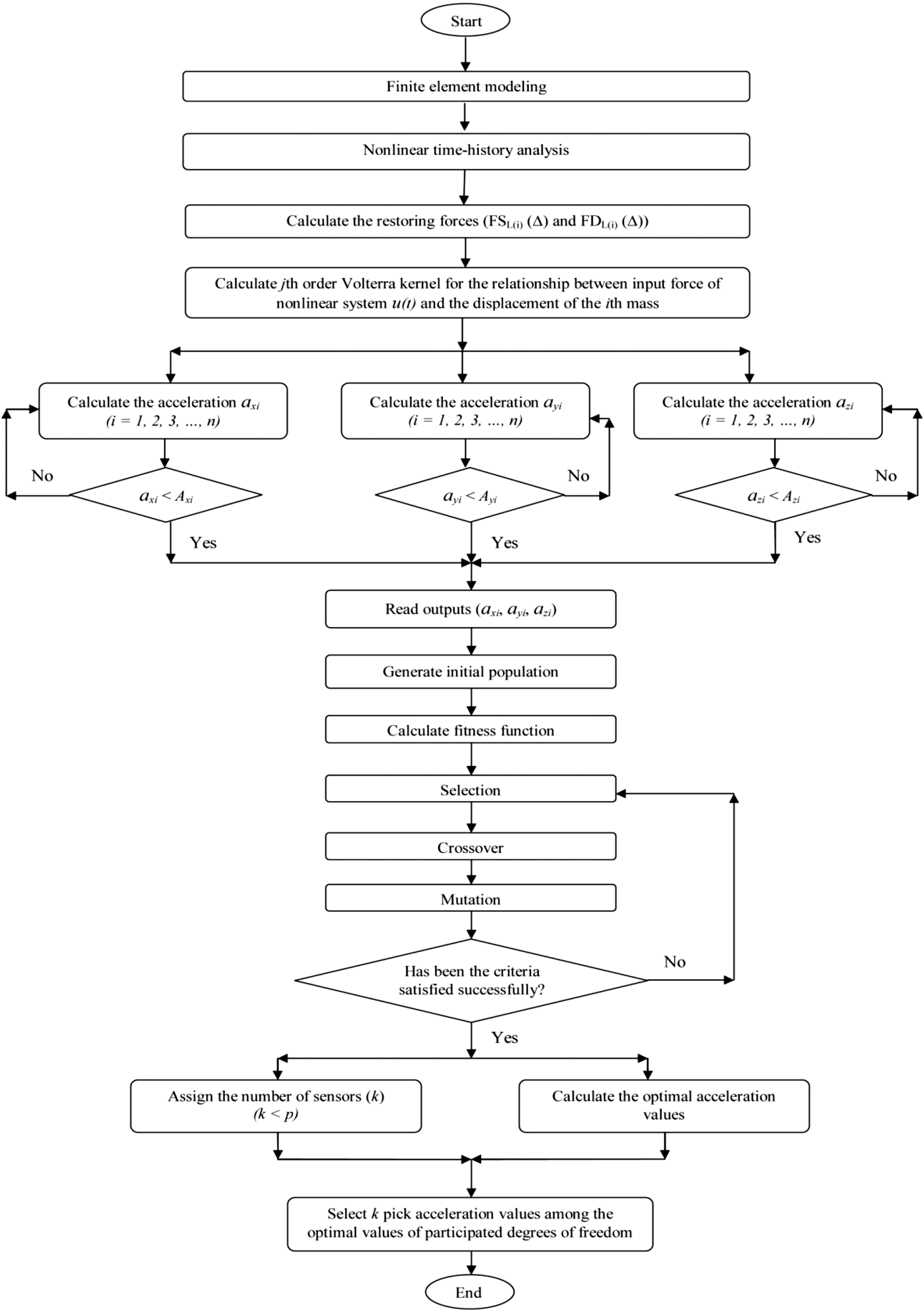
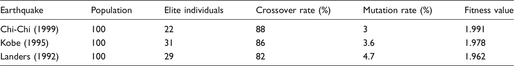
Values of GA parameters.
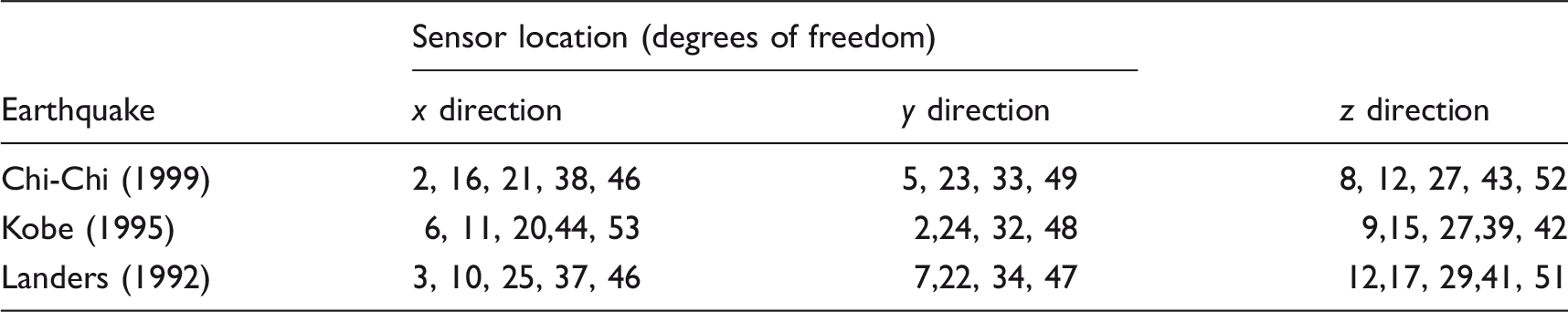
Sensor locations based on the proposed sensor configuration approach.
Sensitivity analysis
In this section, sensitivity analysis is performed with regard to the different number of sensors versus convergence error. To do this, a certain number of sensors are taken into account, e.g. 8 to 24 sensors. Then the proposed algorithm investigates the efficiency of different number of sensors to gain convergence. For each case, the convergence error is computed by the algorithm; see Figure 9 which compares the number of sensors versus convergence error in the piping system under three different earthquakes.
Comparing number of sensors versus convergence error in the piping system.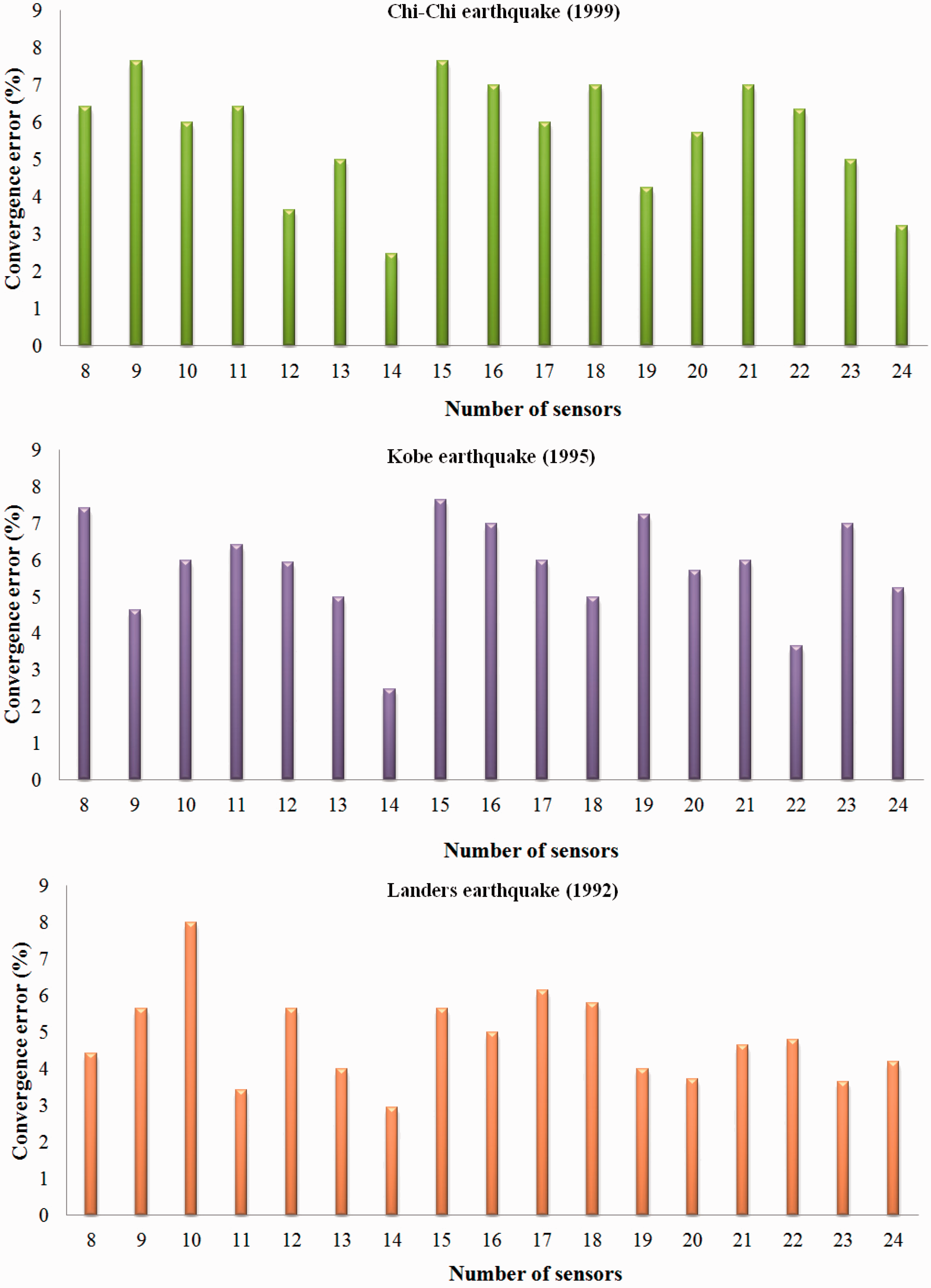
EMAC method
An extended modal assurance criterion (EMAC) approach was proposed by Li
49
to overcome the disadvantages of traditional MAC method with the introduction of a forward–backward combinational approach. The MAC can be defined as equation (15), which measures the correlation between mode shapes
8

In the first step, an intuition sensor set, U0 (including, to say, a number of sensors, S0) is selected. Then, one sensor is added to the initial set until a preset number of sensors, which is somewhat larger than the number of sensors as required, for example, 20% more than required (1.2S0), is reached. This is the same as the forward sequential MAC procedure. The extension differs from the original forward approach in the stopping criterion. The EMAC algorithm is continued to obtain a sensor set, U1, consisting a certain number of sensors (to say, S1,
Secondly, one sensor at each step is excluded from the sensor set U1 until the required number of sensors S0 is reached. This is the backward sequential MAC approach, the essential extension to the forward one. Therefore, two function curves are established. One is the curve of the maximum off-diagonal term with respect to the number of sensors increasing from S0 to S1, which is obtained in the first stage, and the other is the curve of the maximum off-diagonal term with respect to the number of sensors decreasing from S1 to S0, which is found in the second stage. Both curves are compared and the one with a smaller value at the point S0 is selected. In this manner, the maximum off-diagonal term of the MAC matrix may, in many instances, be further minimized than the traditional MAC algorithm. 49
In this paper, the first six modes of the pipeline network are selected and 19 accelerators are taken into account for optimal sensor placement. Table 13 demonstrates the values assigned to reproduction parameters and the attained fitness values for EMAC approach. As the EMAC method relies on the modal analysis results, the effects of seismic ground motions never are considered in the sensor configuration. Figure 10 illustrates the MAC matrix of EMAC method. Also, the sensor locations according to the EMAC are given in Table 14.
MAC matrix of EMAC. Values of GA parameters (EMAC method). Sensor locations for the piping network based on the EMAC method.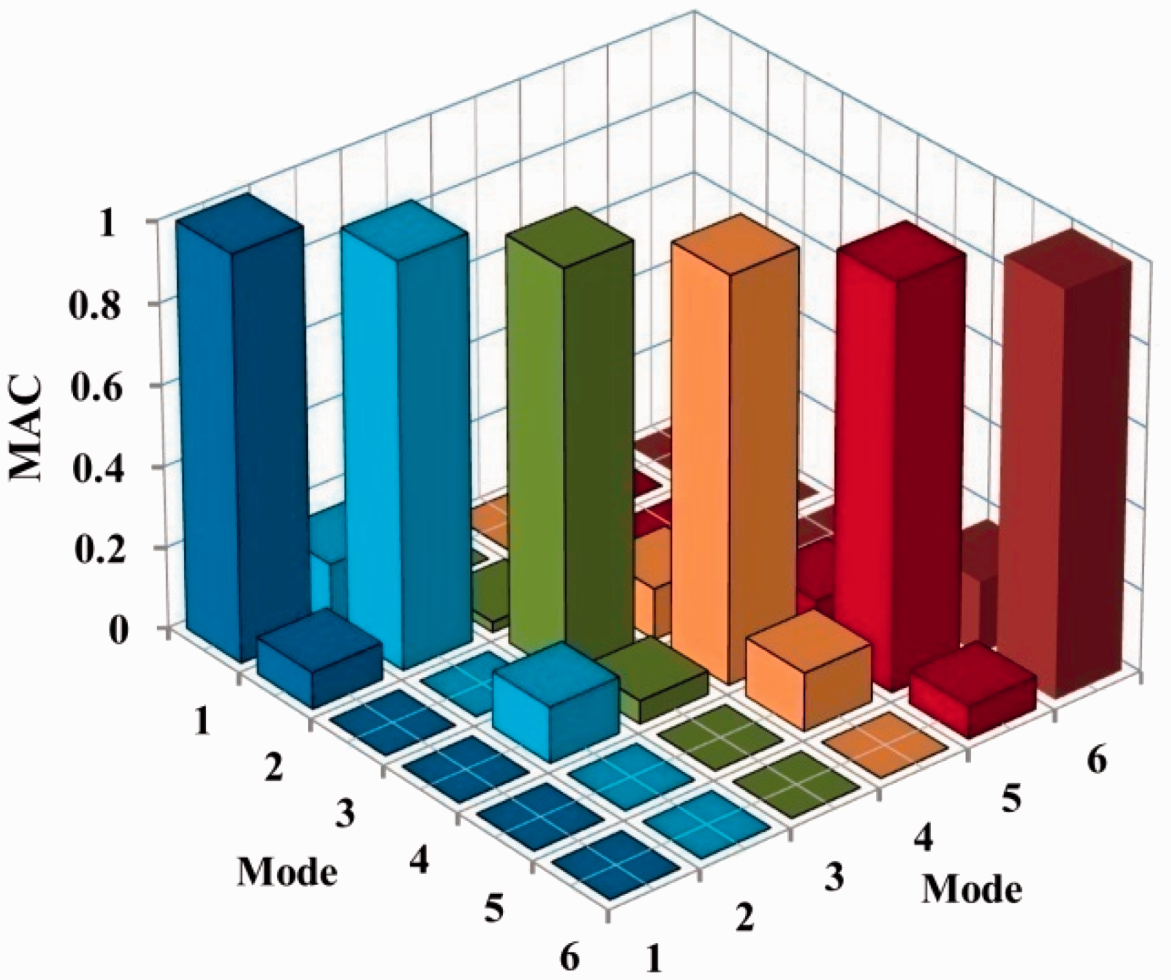


The proposed sensor placement approach vs. DABC algorithm
In this section, the efficiency of the proposed sensor placement is evaluated by comparing this scheme with a new optimal sensor placement method proposed by Sun and Büyüköztürk 50 named discrete artificial bee colony (DABC) algorithm. Sun and Büyüköztürk 50 presented a discrete optimization method to solve the optimal sensor placement problem which they assessed an MAC objective function to estimate the applicability of a sensor placement method in the basis of modal characteristics of a reduced order model. The DABC algorithm improves the continuous artificial bee colony (ABC) method, to solve a discrete type optimization problem.
The ABC algorithm was proposed by Sun et al. 51 to utilize in system identification. The algorithm works by simulating honey bees’ foraging. Three search phases have been represented, naming the Employed Phase, the Onlooker Phase and the Scout Phase. 52 To find more detailed information about the capability of ABC approach in solving inverse problems with continues variables, it is recommended to refer previous researches done by Sun et al.53–55
Sun and Büyüköztürk
50
assumed that the parameter to be optimized is no longer free to vary in a continuous space. They have investigated the effectiveness of the DABC by a numerical example including a 27-bar truss bridge where numerical analyses were done using MATLAB. The truss bridge is a simply supported structure with 27 bars and 15 nodes, while 8 sensors were considered to be installed on the truss bridge. Figure 11 shows the simply supported truss bridge. The material and geometric properties of the truss elements were presented by Sun and Büyüköztürk.
50
Sun and Büyüköztürk
50
also stated that they repeated that algorithm 50 times to solve each problem of optimal sensor placement to prevent solution uncertainty.
Schematic representation of the truss bridge.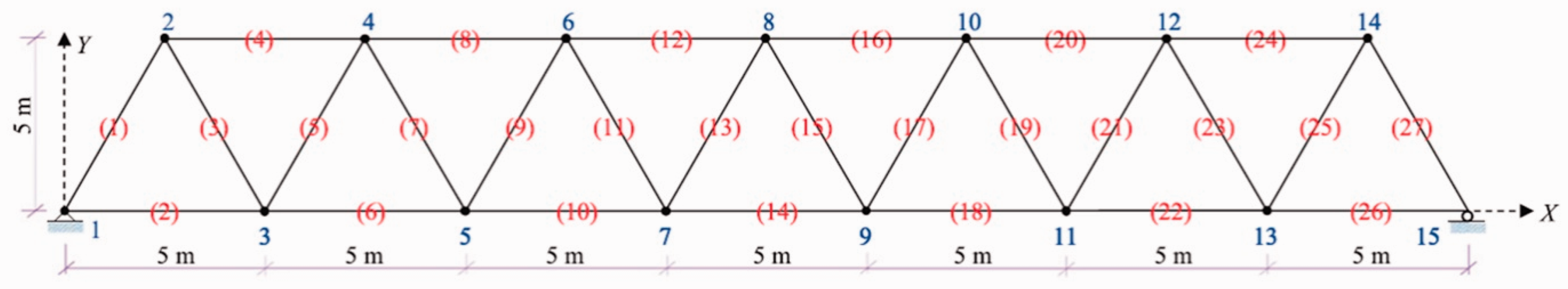
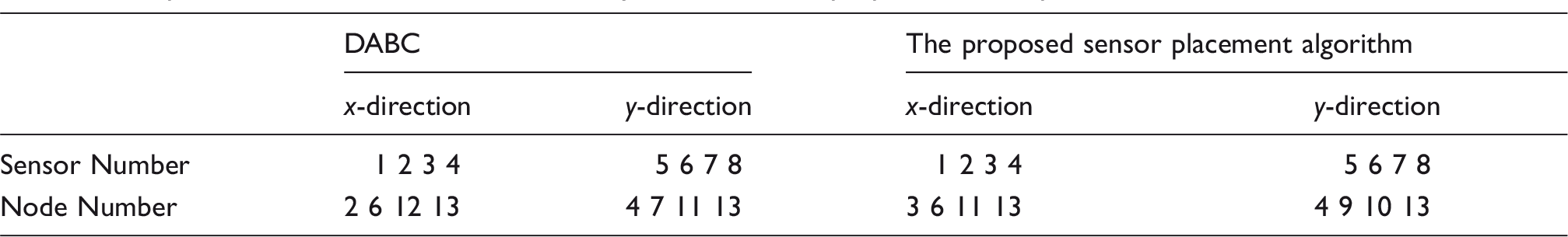
Mann-Whitney test done for comparing convergence results of DABC algorithm and the proposed sensor placement approach.
Optimal locations of sensors obtained by DABC and the proposed sensor placement method.
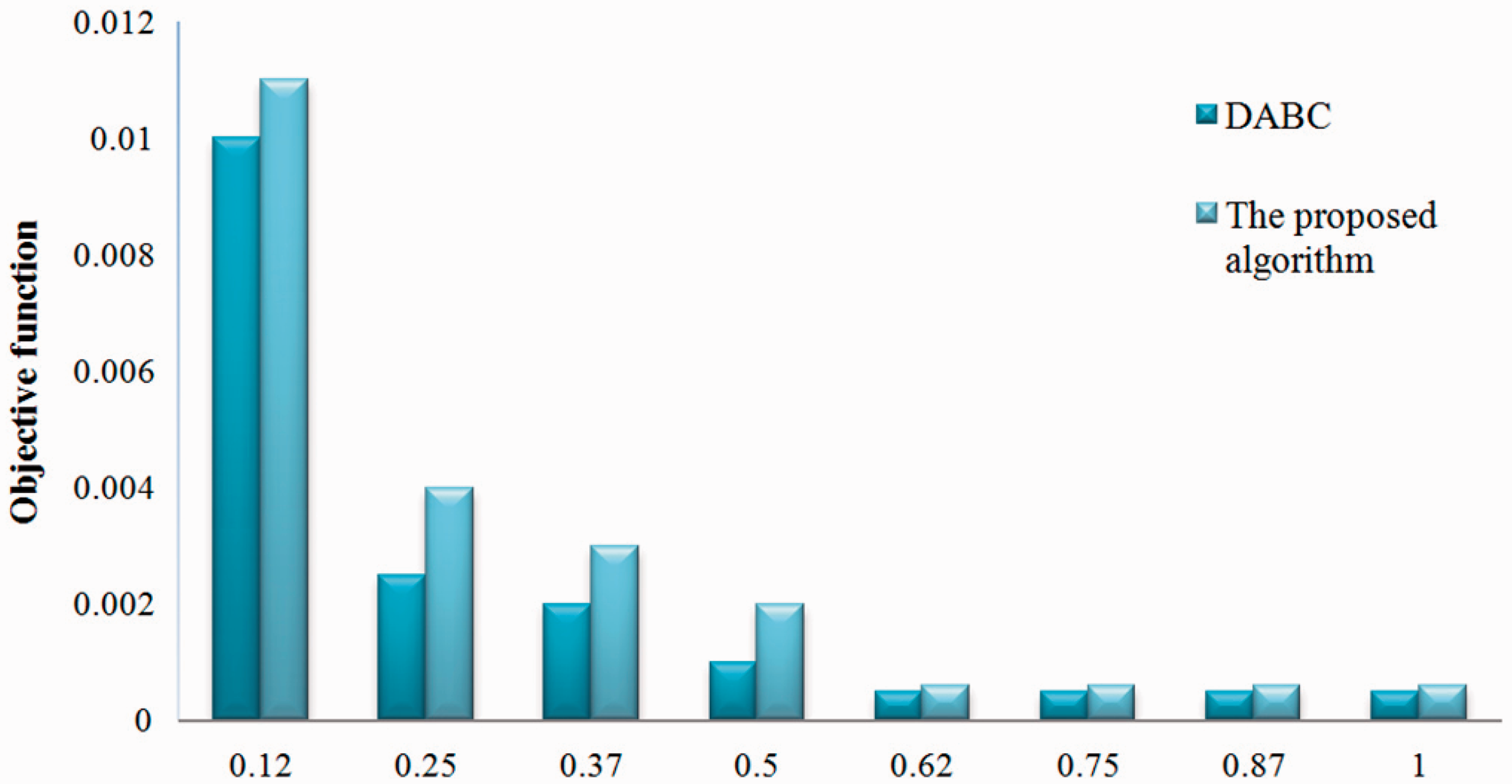
Comparison of convergence for two different optimal sensor placement methods.
Piezoelectric friction dampers
The piezoelectric friction dampers are employed to utilize in the piping system due to their high-speed actuation, low power consumption, reliability, and compactness over a wide frequency range. Because of the nonlinear characteristics of the friction damper used in this study, the establishment of an effective control strategy is a challenging effort.
The friction force of a piezoelectric friction damper is proportional to normal contact force and friction coefficient between two bodies. Normal force of a piezoelectric friction damper is controlled by a piezoelectric stack actuator, and given as
56


Fuzzy logic is typically engaged to define a complicated relationship between a set of inputs and outputs. A fuzzy controller provides the application of this relationship to control the performance of a piping system. The output is the command force of the damper and the force is transformed to voltage to drive the piezoelectric friction damper. A logical range of input variables must be taken into account for input membership functions. If that range is chosen improperly, the membership functions will rarely be applied, and this may exacerbate the performance of the control system. In this study, the maximum value of input membership function engages the maximum velocity of the piezoelectric friction damper.
The Gaussian membership function is utilized for the input variable since it can estimate the most of the other types of membership functions by substituting the parameters given in

The output level, yi, of every rule is assessed by the firing strength, ωi, of the rule. The ultimate output of the system Nfuzzy is inducted by calculating weighted average of all rule outputs, computed as

Optimal damper placement
Exhaustive search method
To ascertain the optimal influence of a given damper placement, it is necessary to indicate the optimum damping and stiffness coefficients. Furthermore, these optimum coefficients for a set of dampers are dependent on both the number of dampers utilized as well as the damper arrangement. Hence, for each damper placement approach, the presented algorithm must optimize the damping and stiffness coefficients. It could be concluded that it can be assumed that all damping coefficients are equal, leading to reduce the damping coefficient selection problem to a one-dimensional problem.24,25
Exhaustive search approach attempts to solve numerical problems in which generate and inspect all data configurations in a large state space that is ensured to include the desired solutions and investigate all possible combinations of number of dampers locations. The mentioned strategy is provided to be globally optimum, but it is an extremely time consuming procedure. In order to assess the optimum effect of damper placement, it is important to indicate the optimal damping and stiffness coefficients. In addition, the optimal damping and stiffness coefficients for a set of dampers are dependent on both the number of dampers used and the location of dampers. Therefore, the algorithm should optimize those coefficients. The optimal stiffness coefficient βopt and optimal damping coefficient Copt can be written as
when Ψ < 1
Step 1: Input seismic records. Step 2: Perform step-by-step nonlinear time history analysis. Step 3: Compute all N possible combinations and set j = 1, where Step 4: j = 1, and set configuration as jth possible case where j < N. Step 5: Calculate the maximum damping force ratio via nonlinear dynamic analysis which performed in Step 2. Step 6: Evaluate the objective function value. Step 7: Choose the most appropriate candidates with the minimum objective function values. Step 8: Set configuration of piezoelectric friction dampers as jth possible case.


Numerical example
Parameters of piezoelectric friction damper proposed by Pardo-Varela. 57
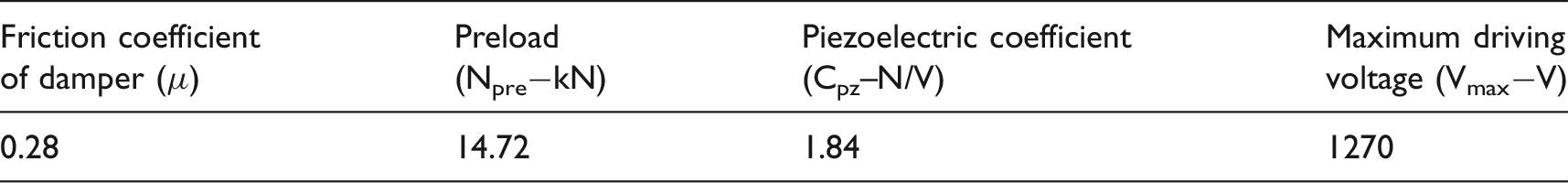
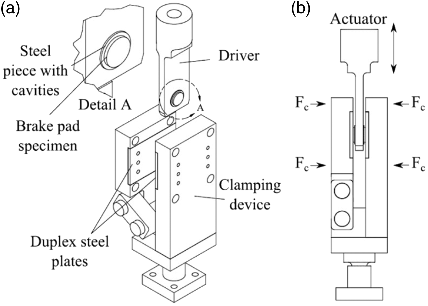
Mechanic system utilized for frictional tests. 57 (a) Parts description and (b) Mechanism closed.
Peak responses of piping system under seismic excitations.
The energy dissipation properties of a damper is often analysed via its hysteresis loop. Figure 14 illustrates the force–displacement hysteretic diagrams for the piping system at node 46 with both vertical and horizontal piezoelectric friction dampers under the seismic waves. It can be seen from the hysteresis diagrams that good amount of energy is dissipated by the piezoelectric friction dampers subjected to three different earthquakes.
Force–displacement diagram for the piping system at node 46 with both vertical and horizontal dampers.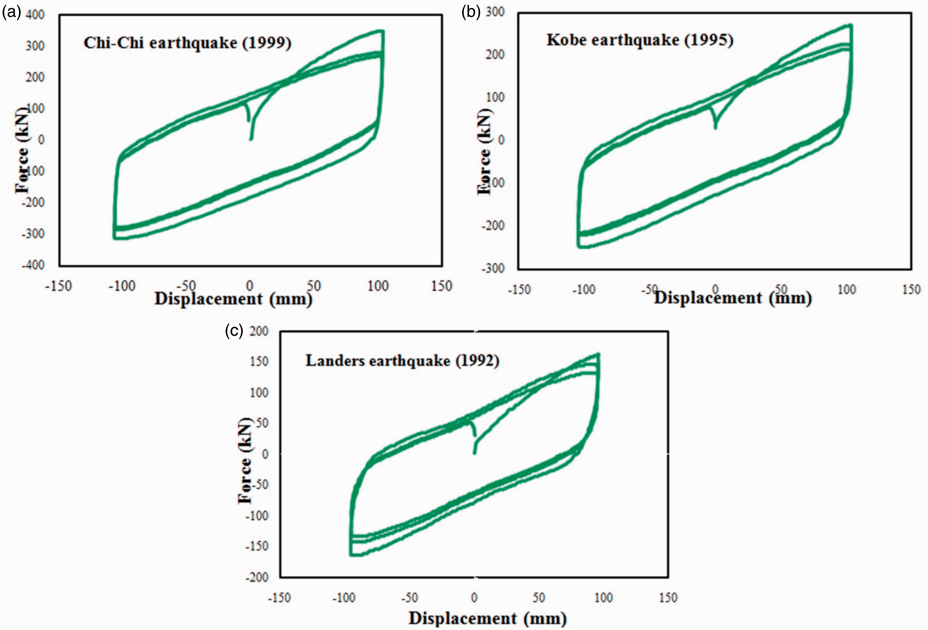
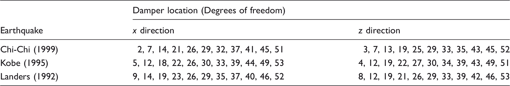
Optimal damper locations.

Deformation of piping system subjected to the 1995 Kobe earthquake.
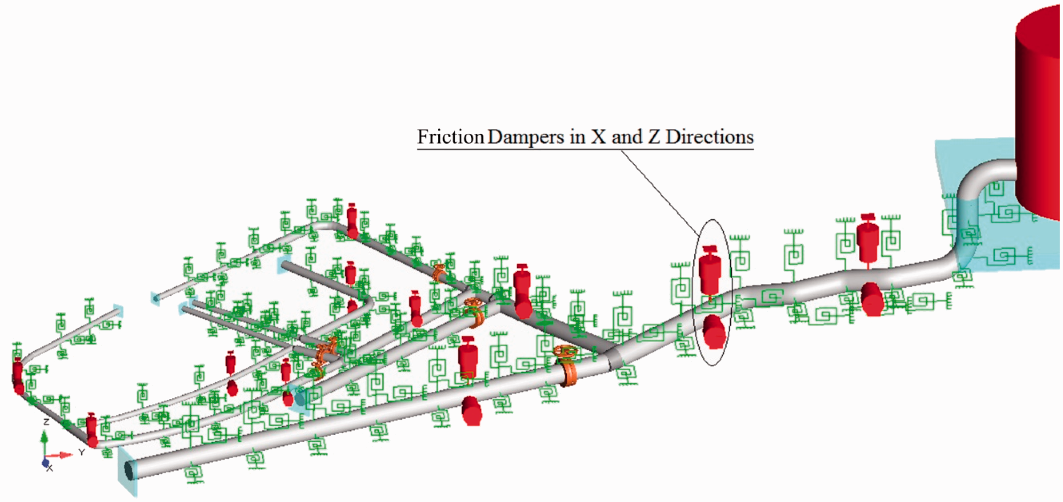
Seismic performance of the system regarding the optimum layout of piezoelectric friction dampers under the 1995 Kobe Earthquake.
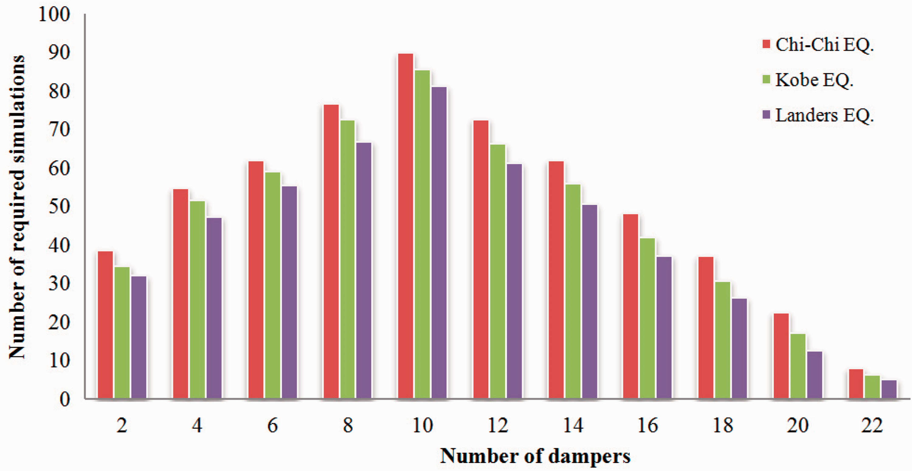
Comparing the number of required simulations and the number of dampers for exhaustive search method.
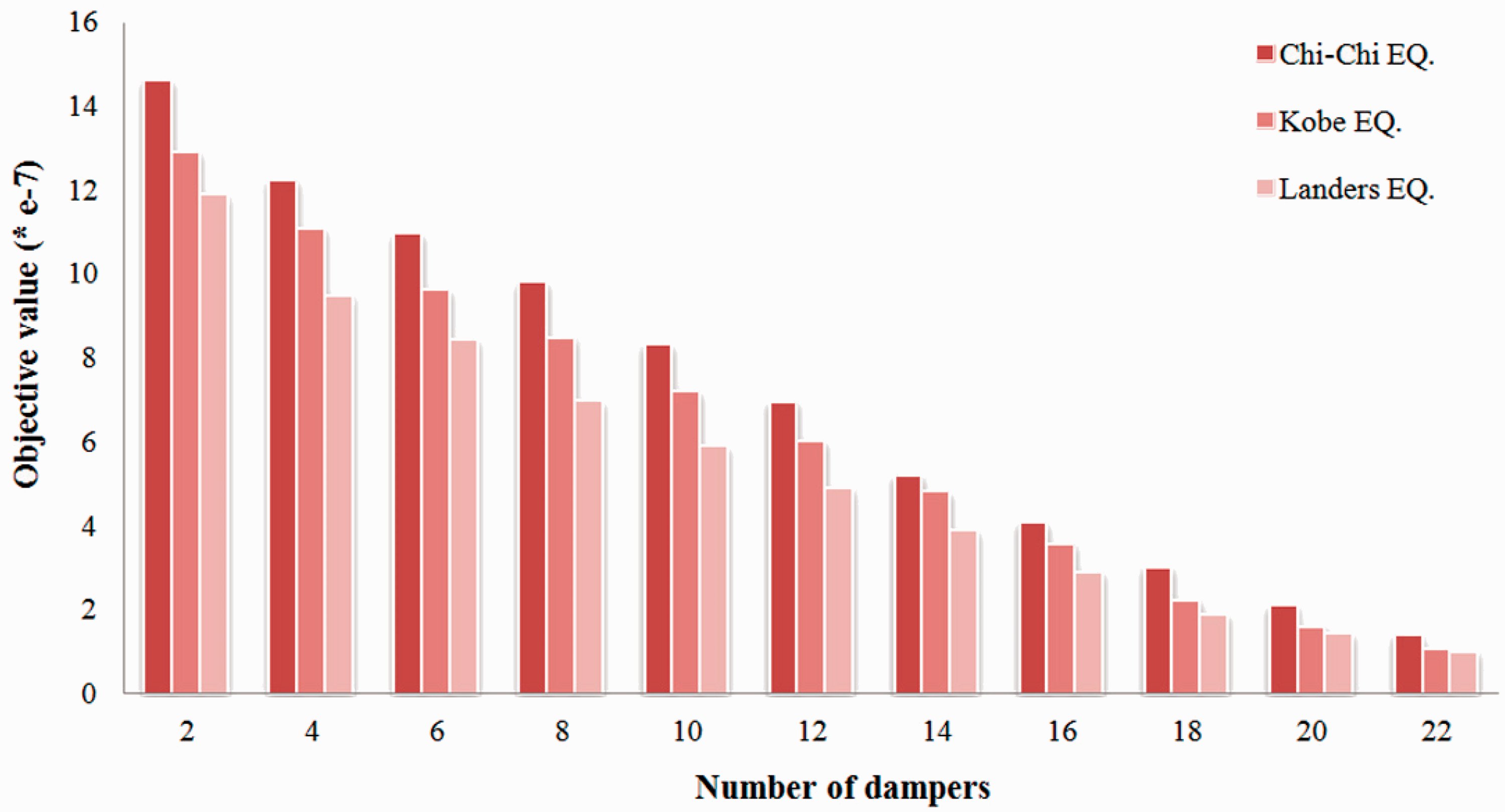
Objective value versus the number of dampers under three different earthquakes
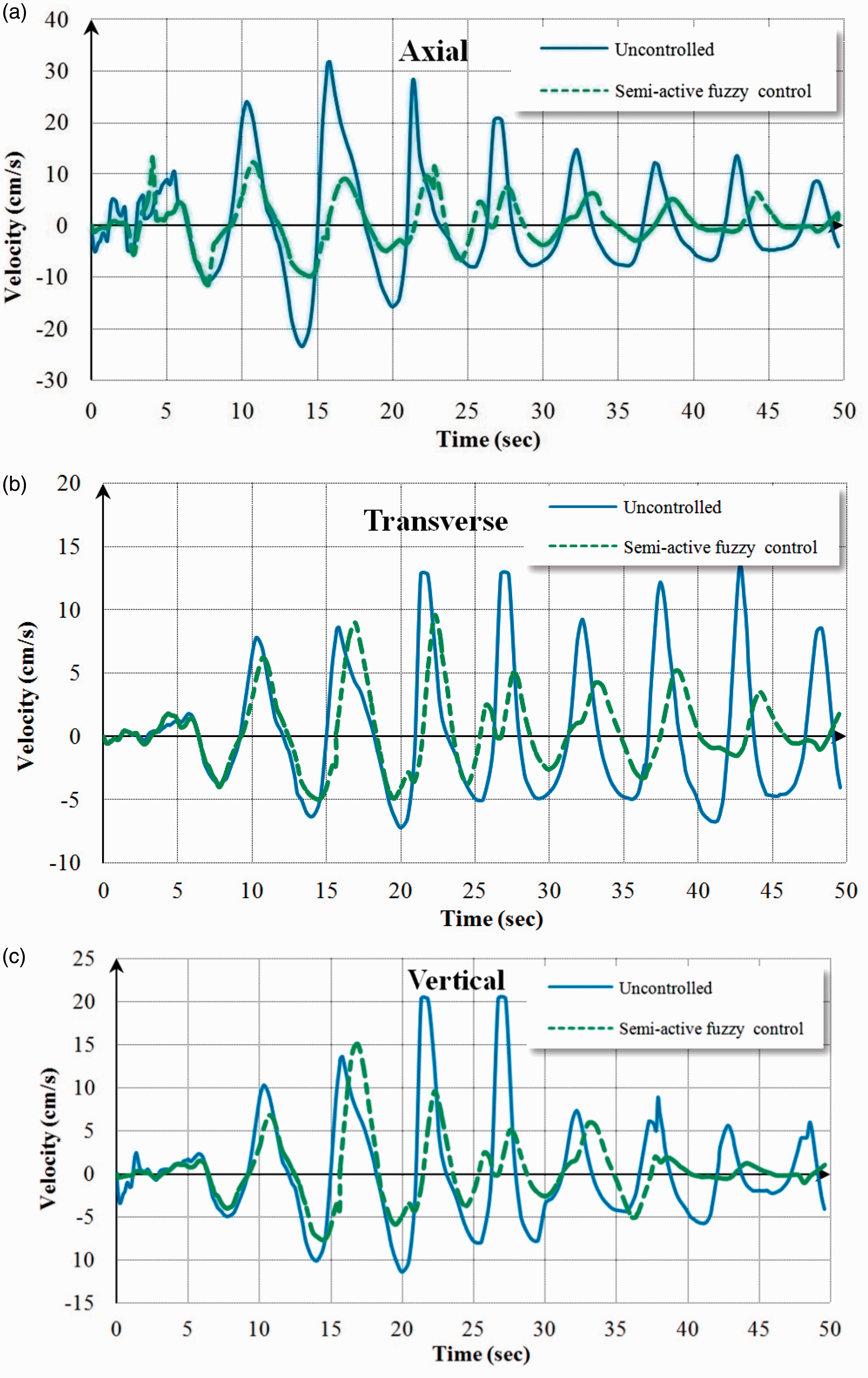
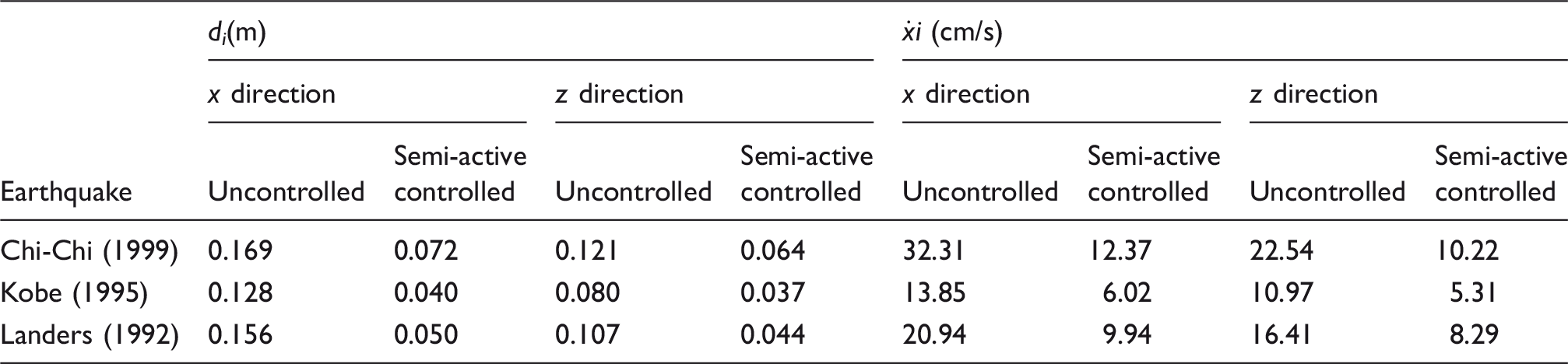
Velocity time histories at node 46 of piping network under the 1995 Kobe earthquake.
Conclusions
The primary objectives of this study include proposing novel strategies for the optimal configuration of sensors and piezoelectric friction dampers to do pipeline monitoring reliably in addition to mitigating earthquake hazards by analyzing the seismic performance of the system in the uncontrolled and controlled conditions. From numerical assessment of the piping system, the following conclusions are drawn:
Three different sensor placement approaches were investigated including the EMAC method, DABC algorithm, and a new strategy proposed by the authors. One of the most important advantages of this new strategy against EMAC and DABC is the accuracy of inputs. To do optimal sensor placement, the EMAC and DABC methods employ modal analysis results, while the new strategy utilizes nonlinear time history analysis results. In the EMAC and DABC, as the input and methodology rely on the linearity, nonlinear components could not be applied in the system, while in the new scheme which is based on Volterra series, a nonlinear MDOF system was presented and an optimal sensor placement was performed using nonlinear dynamic analysis results. In the proposed sensor placement approach, only 14 accelerators were utilized, while 19 accelerators have been employed in the EMAC. Therefore, the number of required sensors in the proposed strategy is 35.7% lesser than the EMAC method. The sensitivity analysis demonstrates that the number of sensors computed optimally by the proposed algorithm contains the least convergence error. From a computer programming point of view, the number of iterations and also the time consumed in the proposed sensor placement method is significantly lesser than the EMAC method. A damper arrangement strategy is presented based on exhaustive search method by optimizing the damping and stiffness coefficients in which the objective function values are compared and, according to the computed minimum value, the corresponding configuration can be obtained. The initial results of nonlinear time history analysis show poor performance of the piping network (see Figure 15), while the secondary time history results demonstrate that seismic energy dissipated efficiently by optimal arrangement of piezoelectric friction dampers in the vulnerable points of the system (see Figures 16 and 19).
Footnotes
Declaration of conflicting interests
The author(s) declared no potential conflicts of interest with respect to the research, authorship, and/or publication of this article.
Funding
The author(s) disclosed receipt of the following financial support for the research, authorship, and/or publication of this article: The authors are grateful for the financial support from National Science Foundation of China under Grant No. 51278219.