In Silico Prediction of Eye Irritation Using Hansen Solubility Parameters and Predicted pKa Values

Abstract

An in silico method has been developed that permits the binary differentiation between pure liquids causing serious eye damage or eye irritation, and pure liquids with no need for such classification, according to the UN GHS system. The method is based on the finding that the Hansen Solubility Parameters (HSP) of a liquid are collectively important predictors for eye irritation. Thus, by applying a two-tier approach in which in silico-predicted pKa values (firstly) and a trained model based solely on in silico-predicted HSP data (secondly) were used, we have developed, and validated, a fully in silico approach for predicting the outcome of a Draize test (in terms of UN GHS Cat. 1/Cat. 2A/Cat. 2B or UN GHS No Cat.) with high validation set performance (sensitivity = 0.846, specificity = 0.818, balanced accuracy = 0.832) using SMILES only. The method is applicable to pure non-ionic liquids with molecular weight below 500 g/mol, fewer than six hydrogen bond donors (e.g. nitrogen–hydrogen or oxygen–hydrogen bonds) and fewer than eleven hydrogen bond acceptors (e.g. nitrogen or oxygen atoms). Due to its fully in silico characteristics, this method can be applied to pure liquids that are still at the desktop design stage and not yet in production.

Introduction

The Draize test and replacement methods

The Draize test (Organisation for Economic Co-operation and Development (OECD) Test Guideline (TG) No. 405) has long been the industry, and regulatory, standard for classifying the irritation potential of chemical substances. ¹ However, due to animal welfare considerations, the Draize test has been heavily criticised for decades and replacement methods have been sought. ² Indeed, a few in vitro assays — for example, the Isolated Chicken Eye (ICE) test, the Bovine Corneal Opacity and Permeability (BCOP) test, the MatTek EpiOcular^™ assay and the SkinEthic^™ HCE ocular irritation assay — have been developed, with the latter three assays having gained OECD acceptance and inclusion in their guidelines. However, all of these methods require either animal tissue or cultured cell lines, and a substantial amount of work in the laboratory is required for each assessment.

In silico models for estimating the eye irritation potential of chemical structures have been developed over the years by using various Quantitative Structure–Activity Relationship (QSAR) and machine learning techniques.^3–8 Many of these models are based on physicochemical descriptors and have good predictive ability. However, the interpretability of the results from such models may sometimes still present a problem for the user. Hansen Solubility Parameters (HSPs) are intuitively understandable, physicochemical substance properties ⁹ that describe the energy from the forces between the molecules according to three parameters: δ_d = energy from dispersive forces; δ_p = energy from polar forces; and δ_h = energy from hydrogen bond forces. As there are three parameters, any substance (e.g. a biopolymer or a liquid) can be conveniently and specifically positioned within a 3-D diagram, when its HSPs (δ_d, δ_p and δ_h) are plotted on separate axes. This allows a pedagogic visualisation of the term ‘like dissolves like’, as substances with similar solubility properties will end up close to each other in this 3-D solubility space. Our research efforts in using HSP descriptors for eye irritation modelling started in 2017. ¹⁰ More recently, another research group has published work on the development of models for classifying compounds as eye irritants or non-irritants.^11,12 However, no external validation with an independent test set was performed in these studies, which limits the value of the models for future predictions of new compounds.

In this article, we present the development, and validation by using an external test set, of an in silico model for the prediction of eye irritation potential for pure liquids from SMILES (Simplified Molecular-Input Line-Entry System) input only. A historical Draize eye test dataset, which was divided into a training dataset and an external test set, was used. HSP descriptors and pKa values were predicted in silico, and a genetic algorithm approach was employed for optimisation of the centre of the HSP sphere, as well as for the sphere radius with negative prediction value as optimisation criteria.

Material and methods

Training dataset

The dataset set was based on historical Draize eye test (OECD TG No. 405) data from the Draize Reference Database (DRD). ¹³ Only pure liquids with no note in the column with the heading ‘Should Not Be Used’, and without the note ‘SCNM’ (meaning ‘Study Criteria Not Met’) in the UN GSH Classification column of DRD were considered for inclusion in the dataset and consisted of 113 compounds (see Table S1 in the Supplemental Material).

Dataset for external validation

External validation of the model was performed by using a dataset taken from the same Cosmetics Europe database, ¹³ applying the same selection criteria as for the training set (see above). The external validation dataset consisted of 40 compounds. In order to allow external validation in terms of classification/no classification according to the UN GHS system, all selected compounds were annotated according to the formal UN GHS Category given in the DRD source. Table S1 (Supplemental Material) contains the full dataset of the compounds used in this study, with the external validation dataset indicated accordingly.

Compound filtering

The File Check function in the HSPiP software ¹⁴ (‘Hansen Solubility Parameters in Practice’; a software allowing Hansen parameter-based calculations, containing a large database of Hansen parameters) was used to remove incorrect SMILES, charged SMILES and small molecules with only 2–3 heavy atoms. These SMILES were removed, as the solubility behaviour of charged molecules is a challenge for all standard solubility tools. In addition, SMILES listed in HSPiP’s Caution output file (which all violated at least one of the ‘Lipinski rule of five’-based criteria by having a molar weight > 500 Daltons, and/or > 5 H-bond donors, and/or > 10 H-bond acceptors) were also removed, as their HSP estimates may potentially be less accurate. Note that a violation of the Lipinski Log P criterion (i.e. Log P of the molecule > 5) does not list a SMILES into the Caution output file, since HSP predictions are considered correct also for very hydrophobic molecules.

HSP parameter predictions

The HSPiP software was used for predicting the HSP parameters for all investigated liquids. ¹⁴ The HSPiP software ¹⁴ (versions 5.0.06-5.3.08) was used for obtaining in silico-predicted HSP parameters for all investigated liquids. All of the HSP data used in this study were predicted directly from the 2-D structure (SMILES) of the liquids only, either via the Y-MB module present in the DIY section of HSPiP, or via direct download from the ‘10k’ database in HSPiP, which contains HSP values for ca 10,000 compounds, pre-predicted from SMILES by using the same algorithm as that used in the Y-MB module. The Y-MB method is a group contribution method, where the contributions have been optimised via a neural network to fit not only to canonical HSP values but also to experimental datasets with values deeply related to HSP values such as Trouton constants, densities and refractive indices. The algorithm for HSP prediction has stayed unaltered in the versions of HSPiP described above and used in this study. The accuracy of the predictions from the licensed HSPiP software is unknown, but will be reflected in the predictive performance of the model.

pKa predictions

In silico-predicted pKa values of the compounds and/or in silico-predicted pKa values for their corresponding acids, were obtained by performing a manual online search in SciFinderⁿ based on the CAS number of each compound. ¹⁵ All pKa values found were predicted by Advanced Chemistry Development (ACD/Labs) Software V11.02 (© 1994–2021 ACD/Labs). See Figure S1 in the Supplemental Material for further details of the pKa calculation.

Genetic algorithm optimisation

The genetic algorithm (GA) method ¹⁶ used in this work was downloaded from pypi ¹⁷ and wrapped in a similar manner as described in the GitHub repository rmsolgi/geneticalgorithm ¹⁸ for continuous variables — in our case, the continuous variables to be optimised by the algorithm were the coordinates for the three HSP parameters and the radius of the HSP sphere.

The training set of 108 compounds, after the pKa-filtering out of five compounds, was, for each GA optimisation restart and loop, split in a randomly stratified manner into a second training set (2/3) for building the HSP sphere, and a internal testing/calibration set (1/3) for evaluating the outcome of the optimisation. The negative predictive value with prevalence (0.26 for Cat. 1 + Cat. 2A + Cat. 2B) ¹⁹ was used as the optimisation criterion to be maximised, so that the model does not err on the side of negative predictions, i.e. false negatives. The respective median values in the training set for the three HSP parameters (δ_d, δ_p and δ_h) were used as starting values for the optimisation. The maximum allowed HSP sphere radius was increased during three different runs (loop = 0–2) according to the formula:

radiimax = (loop + 1)*5 + 5

The following GA parameters were used during the optimisation:

— ‘max_num_iteration’: 100

— ‘population_size’: 100

— ‘mutation_probability’: 0.2

— ‘elit_ratio’: 0.0

— ‘crossover_probability’: 0.5

— ‘parents_portion’: 0.3

— ‘crossover_type’: ‘uniform’

— ‘max_iteration_without_improvement’: 5

Ten complete restarts of the GA optimisation were performed for each run (loop). For each GA function evaluation, the following information was collected: the output values for the optimisation function; the three HSP parameters; the radius of the HSP sphere; as well as the number of false positives, true negatives, true positives, false negatives, sensitivity, specificity and balanced accuracy for both the training and calibration set, respectively. After the completion of the GA procedure (runs and restarts), the number of GA evaluations was filtered so that the results for specificity (SP) and negative predictive value (NPV) for the training set did not outperform the corresponding results for the calibration set by more than 0.1 — i.e. the differences between the training and calibration set results for SP and NPV, respectively, were ≤ 0.1.

In order not to err on the side of negative predictions, the HSP parameters for the model where the calibration set showed the highest sensitivity and, secondly, the highest specificity was chosen for predicting the outcome of the external test set.

Applicability domain determination

The applicability domain for the developed model was determined with the k-nearest neighbours (KNN) method. ²⁰ In the KNN approach, distances among data points are calculated by using various distance measures, such as the Euclidean distance in this case. For each training set point, its distance to its kth neighbour (in our case, k = 20) in the HSP space, i.e. the three HSP parameters, was identified. By following this procedure, we collected Euclidean distances to the 20th neighbour for each of our training set points. Finally, we calculated the 95th percentile score from these distance values, which was considered as a threshold (outlier) score. In the end, for any new query, we first calculated its Euclidean distances with our training set data points. If the distance to the 20th closest neighbour was lower than or equal to our threshold (outlier) score (see Model performance section), it was labelled as an inlier, otherwise it was considered to be an outlier. Also, it should be noted that the model in its current form is formally applicable only to the types of substances that were used to train and validate it; these substances comprise pure non-ionic liquids with:

— no more than five hydrogen bond donors (e.g. nitrogen–hydrogen or oxygen–hydrogen bonds);

— no more than ten hydrogen bond acceptors (e.g. nitrogen or oxygen atoms); and

— a molecular weight below 500 g/mol.

Solids were excluded from both the training and validation sets of the prediction model for two reasons. Firstly, their solubility cannot always be correctly predicted via HSP alone (as solubility also depends on melting point and enthalpy of fusion) and, secondly, solids may also irritate the eye mechanically if not dissolved. To avoid this complication in this first version of our eye irritation model, we decided to omit solids from the applicability domain of this model.

Results and discussion

As noted previously by the first author, ¹⁰ there is a relationship between eye irritation and the position of a liquid in the HSP space. This was also confirmed by Fujii et al. ¹¹ and by Ito et al. ¹² However, none of these three investigations applied any rigorous statistical analysis with associated validation processes to the developed models, which would be required for the use of such models in industry or for the wider benefit of society, e.g. via their inclusion in OECD guidelines with the aim of reducing the number of animal experiments performed. The outcomes from such a rigorous analysis of the model, including its external validation, are presented here.

Addition of the pKa criterion

The OECD Guidance Document No. 263, on Integrated Approaches to Testing and Assessment (IATA) for serious eye damage and eye irritation, ²¹ states that test chemicals having pH ≤ 2.0 or pH ≥ 11.5 are predicted to cause serious eye damage (UN GHS Cat. 1) as a direct result of having a pH above/below these threshold values. Therefore, they should not be evaluated in the Draize test, but instead be directly classified as UN GHS Cat. 1. ²¹ Based on this guideline — and on the fact that the position in HSP space for a given pure liquid only gives information of the liquid’s polarity/solubility properties and no information on its acidic or alkaline properties — we wanted to improve our model by adding a criterion for the direct classification as an irritant, based on the predicted pKa value for a given pure liquid (or for its corresponding acid, in the case of an alkaline compound). See Supplemental Material Figure S1 for a more detailed description of this rationale.

Training of a model for the prediction of pure liquids

In this investigation, we attempted to fit a sphere in the HSP space corresponding to the liquids in Table S1 that are denoted as the training set, excluding compounds for which the outcome was predetermined by the pKa criterion, with the expectation that positive liquids (Cat. 1, Cat. 2A, Cat. 2B) will be clustered inside the sphere and the negative liquids (No Cat.) will be found outside of it.

The sphere-fitting was performed as described above (see the Materials and methods section), based on three runs with increasing maximum allowed sphere radius as well as ten complete restarts of the GA procedure during each run. From this, a sphere was obtained, with the coordinates and radius in HSP-space as shown in Table 1.

Table 1.

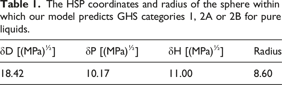
The HSP coordinates and radius of the sphere within which our model predicts GHS categories 1, 2A or 2B for pure liquids.

δD [(MPa)½]	δP [(MPa)½]	δH [(MPa)½]	Radius
18.42	10.17	11.00	8.60

Model performance

The potential models for evaluation were limited due to the unbalanced performance of the training set versus the calibration set with respect to differences in specificity (SP) and negative predictive value (NPV), respectively. This, in combination with the desired goal of the model not to err on the side of negative classifications (i.e. false negatives), resulted in the selection of a model with the highest sensitivity (SE), followed by the highest SP for the calibration set. The results from validation on the external test set are presented in Table 2 (pKa criterion-predicted liquids included, and outliers excluded).

Table 2.

A summary of the performance of the in silico HSP/pKa model for the external test set.

False positives (FP)	True negatives (TN)	True positives (TP)	False negatives (FN)	Sensitivity (SE)	Specificity (SP)	Balanced accuracy (BA)
4	18	11	2	0.846	0.818	0.832

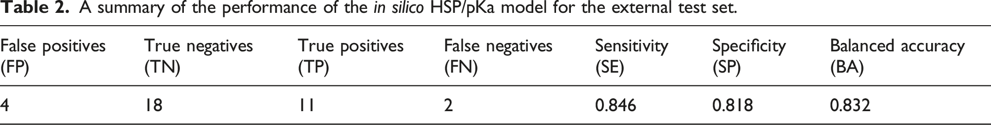
The HSP model correctly predicted 18 out of 22 negative (No Cat.) liquids, as well as 11 out of 13 positive (Cat. 1, Cat. 2A and Cat. 2B) liquids. The pKa criterion correctly identified, via their extreme pH, three out of the 13 positive liquids as irritants; no incorrect predictions were made using the pKa criterion. The applicability domain procedure identified five liquids in the external test set as outliers at a threshold (outlier) score of 1.42 derived from the training set. These outliers are not included in the results presented in Table 2. Of the five outliers, four were designated as negative (No Cat.) and one as positive (Cat. 2A). The positive outlier was correctly classified by the model, as well as three out of the four negative outliers.

Sensitivity describes the model’s potential to classify a positive chemical into the positive class, while specificity indicates the model’s potential to classify a negative chemical into the negative class. When predicting the external test set, the sensitivity and specificity of the model were 0.846 and 0.818, respectively, while the balanced accuracy (BA), which is the arithmetic mean of sensitivity and specificity, was 0.832.

To understand the model’s potential to incorrectly classify chemicals, we evaluated the false positive rate (FPR), as well as the false negative rate (FNR). The FPR is the proportion of the negative class (i.e. No Cat.) chemicals that the model has classified as positive, whilst the FNR is the proportion of the positive class (i.e. Cat. 1, Cat. 2A and Cat. 2B) chemicals that model has classified as negative. The FPR and FNR scores were 0.182 and 0.154, respectively. A positive predictive value (PPV) gives the probability that a positive result obtained by our model is correct, whereas a negative predictive value (NPV) describes the probability that a negative result is correct. The PPV and NPV scores (at prevalence 0.26, see above) were 0.620 and 0.938, respectively. The starting objective for this model building exercise, as mentioned earlier, was not to err on the negative side of predictions, i.e. the FNR should be minimised. The FNR calculated from the external validation of our model (see above) indicate that this objective has been achieved.

Conclusions

The work presented in this investigation has resulted in the development of a fully in silico-based method that permits the rapid prediction of eye irritation potential for pure liquids by using Hansen Solubility Parameters. This represents the addition of a well-calibrated and validated method to the new approach methodology (NAM)-based predictive toolbox, for use in the important area of industrial safety assessment. Furthermore, as the negative predictivity of the model is high, we therefore propose that the method could potentially be used in situations where non-eye irritants need to be identified from a set of candidate molecules — with the added benefit that the screening could be performed before the physical existence of the liquid itself, i.e. at the desktop design stage of, for example, a fragrance or pharmaceutical candidate molecule. This would clearly contribute to the emerging ‘safe by design’ aims of the EU Chemical Strategy for Sustainability (CSS). ²²

Supplemental Material

Supplemental Material - In Silico Prediction of Eye Irritation Using Hansen Solubility Parameters and Predicted pKa Values

Supplemental Material for In Silico Prediction of Eye Irritation Using Hansen Solubility Parameters and Predicted pKa Values by Martin Andersson, Ulf Norinder, Swapnil Chavan and Ian Cotgreave in Alternatives to Laboratory Animals

Supplemental Material

Supplemental Material - In Silico Prediction of Eye Irritation Using Hansen Solubility Parameters and Predicted pKa Values

Supplemental Material for In Silico Prediction of Eye Irritation Using Hansen Solubility Parameters and Predicted pKa Values by Martin Andersson, Ulf Norinder, Swapnil Chavan and Ian Cotgreave in Alternatives to Laboratory Animals