
Abstract

Traditionally, investment management consisted of (a) asset allocation (how much to invest in stocks and how much in safer assets like bonds) and (b) security selection (which stocks to buy and sell). The asset allocation decision can be implemented in a passive way: it is possible to buy an indexed fund that provides exposure to equity market without worrying about individual stock picking decisions at all. The second decision (security selection) is inherently a process of active management which involves taking a view on the prospects of individual companies. In recent decades, considerable attention has been focused on factor investing, 1
Factor investing is also sometimes referred to (particularly in marketing brochures) as smart beta, exotic beta, or alternative beta.
The increasing focus on factor investing is also driven by an explosion of academic literature on factor models, but it is important to remember that factor models are largely based on data and are only weakly grounded in theoretical considerations: they are ‘empirical asset-pricing models; that is, they try to capture the cross-section of expected returns without specifying the underlying economic model that governs asset pricing’ (Fama & French, 2012, p. 458). The empirical asset pricing models clearly reflect real world phenomena and not just the theoretical assumptions of the modeller. But the empirical foundation is also a weakness of factor models because of the grave risk of data mining. Recent literature has emphasized this worry. Cochrane (2011) complained about ‘a zoo of new factors’; Harvey, Liu and Zhu (2016) provide evidence that about half of the published factors are false discoveries, and Hou, Xue and Zhang (2015) arrive at a similar conclusion.
A conservative approach to the application of factor models is, therefore, appropriate. First, it makes sense to focus on the long established factors that have been exhaustively tested across a wide range of countries and time periods. The size, value, and momentum factors put forth by Fama and French (1992, 1993, 1996), Jegadeesh and Titman (1993), and Carhart (1997) are among the best-established factors. Not only have they been tested in a range of developed markets (Fama & French, 2012) but there is considerable evidence in favour of these factors in a range of emerging markets as well (Cakici, Fabozzi, & Tan, 2013; De Groot, Pang, & Swinkels, 2012; Eun et al., 2010). Second, it is prudent to study the performance of factor models in each country separately without assuming that what works in some countries will work in others. This article looks at the performance of the four factor model in India in the post-reform period. Due to data limitations, our study covers the period from 1 January 1994 to 31 March 2017, spanning nearly 25 years.
The definition of the size, value, and momentum factors, and the methodology for their construction in the Indian equity market are described briefly in Annexure 1; more details are available in our working paper (Agarwalla, Jacob, & Varma, 2013). The time series of the factors and the underlying portfolios are available in an online data library (Agarwalla, Jacob, & Varma, n.d.) in a manner analogous to the Fama–French data library (French, n.d.).
MAJOR EVENTS IN THE EQUITY MARKET
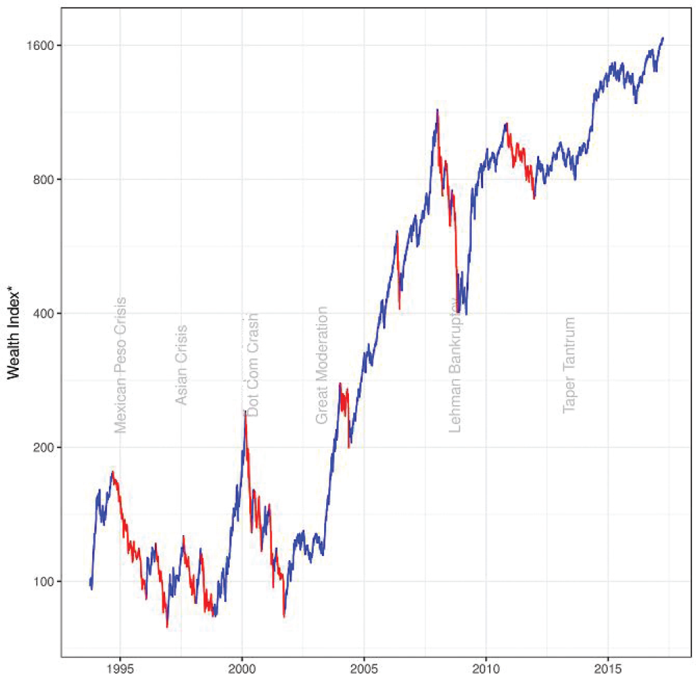
The first decade in our sample data was not a good one for the Indian equity markets, as it was hit by a succession of adverse global shocks: the Mexican peso crisis, the Asian crisis, and the dot-com crash. The subsequent period has been much better. Figure 1 shows the bull (blue) and bear (red) phases of the market. 2
The market for our purposes includes all the stocks in our liquidity-filtered sample and not just the Nifty or Sensex stocks. Moreover, the market return has been calculated after taking dividends into account. For these two reasons, the growth in the wealth index of the market differs from the growth rate of the Nifty or Sensex over the same period.
EQUITY RISK PREMIUM
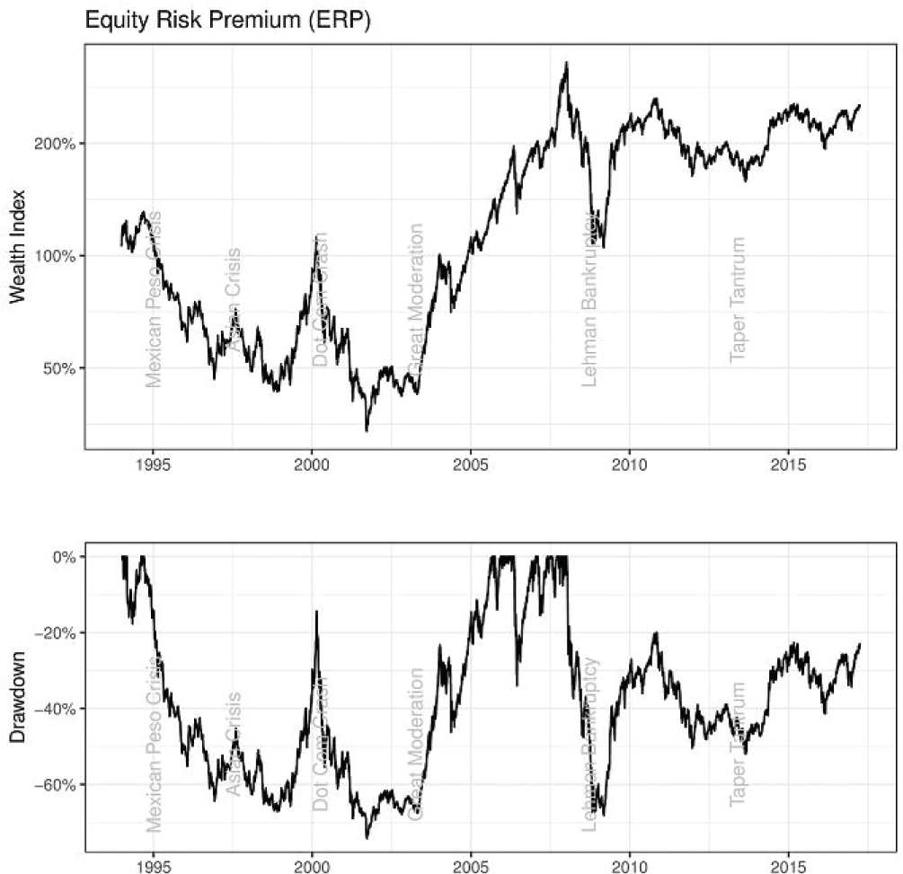
Equity Risk Premium (ERP) is defined as the excess of the return in the stock market over the risk-free rate. ERP provided an annualized return of 4.1 per cent with an annualized volatility of 22.8 per cent. The worst drawdown 3
Drawdown refers to the loss suffered when the value of a portfolio declines from its previous peak. For an investor who is unfortunate enough to have invested at the peak, the depth of the drawdown (percentage decline from the peak to the ensuing trough) is the loss (of principal and/or risk free interest) that he would sustain, if s/he exits at the worst point of time. The duration of the drawdown (time taken to reclaim the previous peak) is the period that the unfortunate investor would have to wait to get back his principal along within risk free interest, if s/he holds on to the investment.
VALUE FACTOR
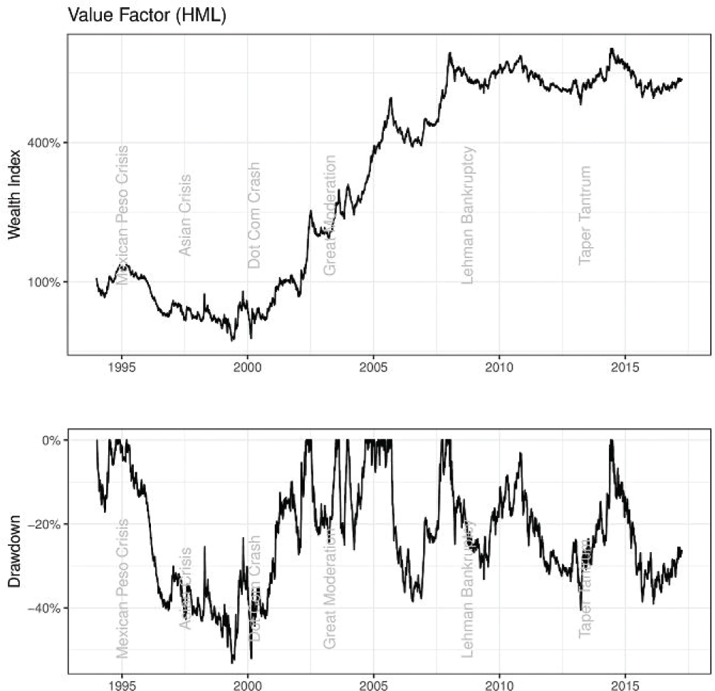
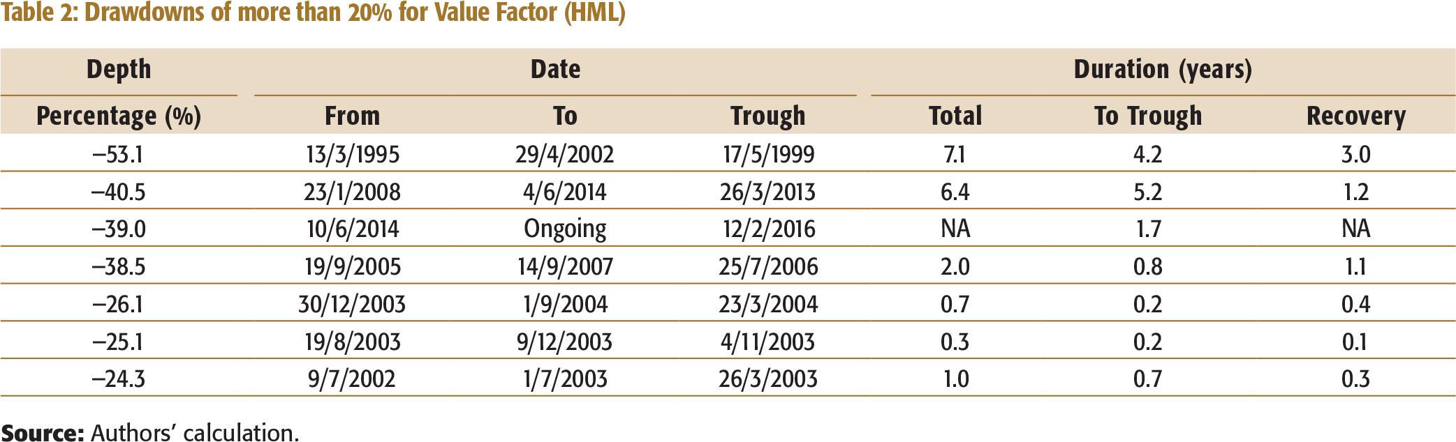
The value factor (also referred to as high minus low: HML) provided an annualized return of 9.08 per cent with an annualized volatility of 16.33 per cent. The value premium is greater than the value premium reported by Fama and French (2012) for the global markets. At the same time, it is comparable to the premium obtained for the emerging markets by (Cakici, Fabozzi, & Tan, 2013). As in the case of the ERP, the value factor also experienced its worst drawdown (53%) during the mid-1990s and early 2000s, encompassing the Mexican peso crisis, the Asian crisis and the dot-com bust (Figure 3 and Table 2). The drawdown was not as deep as that for the ERP and the duration of the drawdown (7.1 years) was also shorter than for the ERP. The second worst drawdown was after the global financial crisis, and again the depth and duration of the drawdown were milder than that for the ERP.
However, value is characterized by a large number of shallow and short drawdowns. There were 7 drawdowns of more than 20 per cent with a median duration of 2 years.
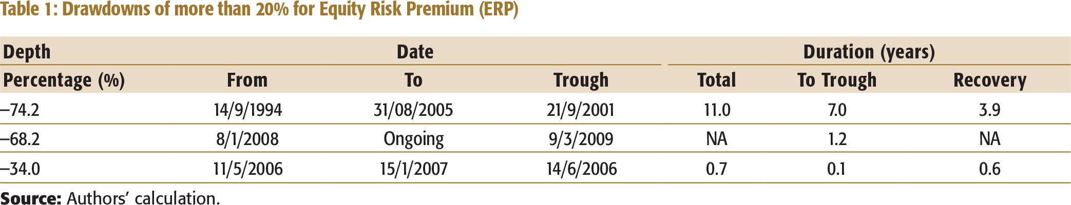
Drawdowns of more than 20% for Equity Risk Premium (ERP)
Drawdowns of more than 20% for Value Factor (HML)
Size factor
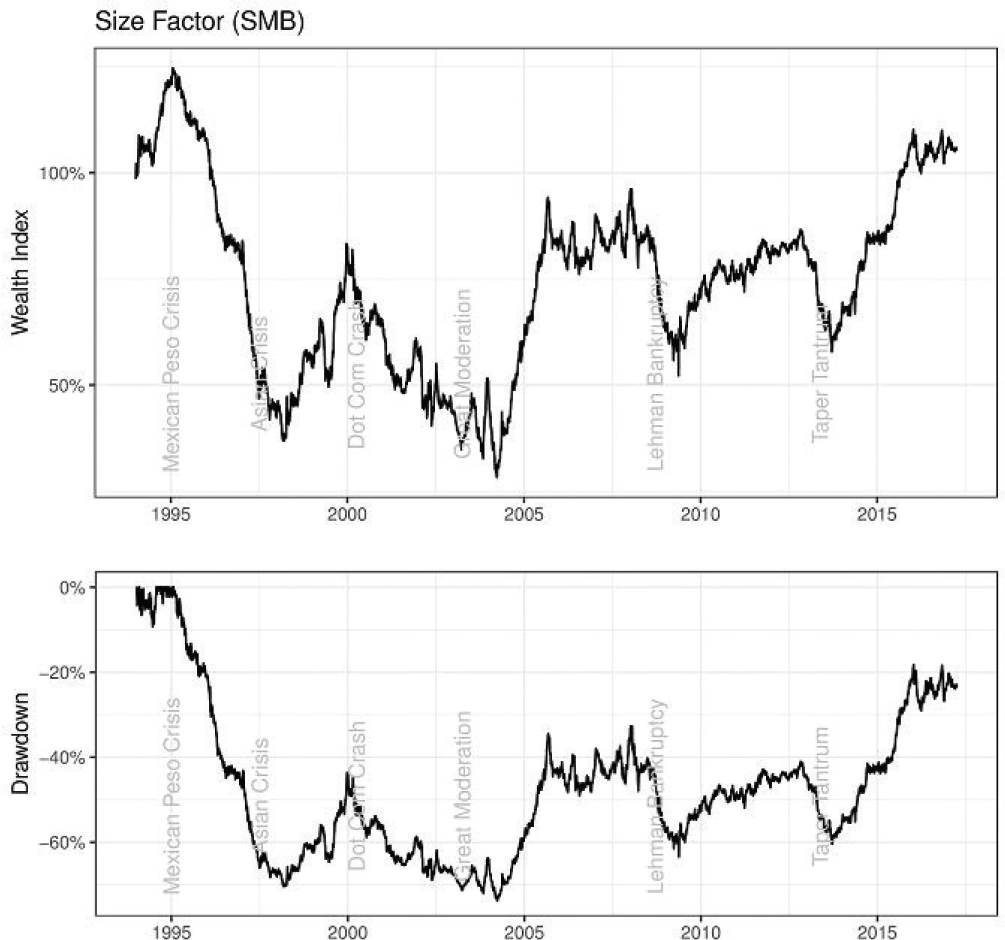
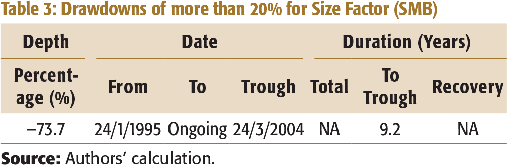
The size factor (also referred to as small minus big: SMB) provided an annualized return of 0.36 per cent with an annualized volatility of 14.51 per cent. The economically insignificant size factor returns obtained here contrasts with the significant returns reported by many other studies, including (Fama & French, 2012) for the developed markets and (De Groot, Pang, & Swinkels, 2012) for the emerging markets. The miserable performance of the size factor in India is due to a steep decline in the wealth index during the mid-1990s, from which the factor has not recovered even after two decades (Figure 4 and Table 3). From peak to trough, the drawdown was 74 per cent. The decline phase of this drawdown is similar to that of the ERP and the value factor during the same period, but unlike these factors, the size factor never recovered from the decline. It is possible that there were structural changes in the Indian market associated with the dominance of foreign portfolio investors which made this factor a poor investment strategy in the 21st century.
Drawdowns of more than 20% for Size Factor (SMB)
Momentum factor
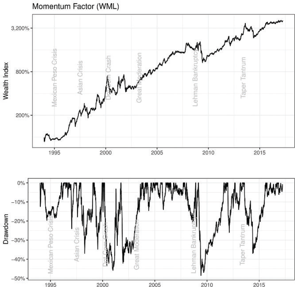
The momentum factor (also referred to as winners minus losers: WML) provided an annualized return of 17.3 per cent with an annualized volatility of 17.06 per cent. The magnitude of the momentum factor return is somewhat greater than those reported from emerging and developed markets around the world. Momentum is, by far, the best performing of all the factors.
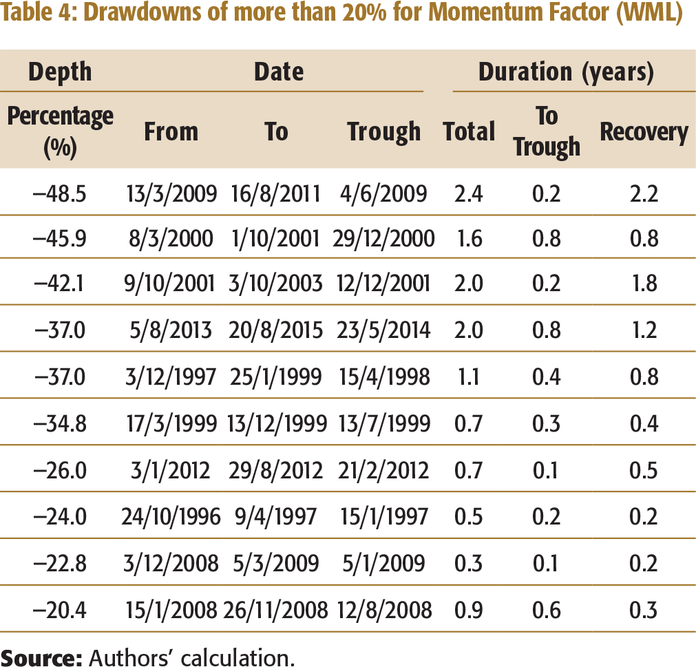
Momentum is characterized by many short and shallow drawdowns (Figure 5 and Table 4). There were 10 drawdowns of more than 20 per cent. The median duration of a drawdown was 1 year, while the maximum drawdown duration was 2.4 years. The worst drawdown (49%) occurred during the post-global financial crisis rally and lasted 2.4 years.
Globally, it is well known that momentum tends to underperform during sharp rallies that follow a market crash, and that is what we observe in India as well.
Drawdowns of more than 20% for Momentum Factor (WML)
EFFICIENT FRONTIERS
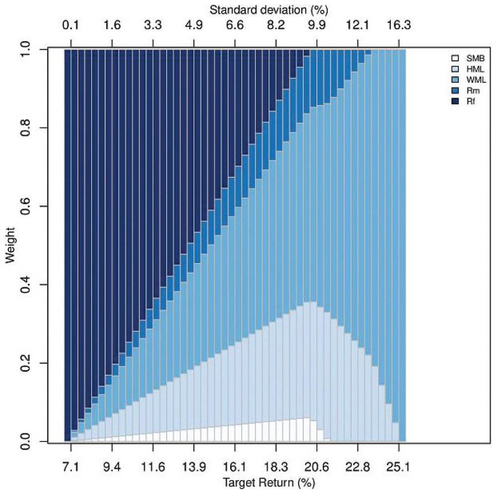
It is more meaningful to look at the optimal allocation of a portfolio considering the various risk factors, instead of looking at each factor in isolation as has been done earlier. We first look at allocating the total portfolio between the risk-free assets and the four factors (market, size, value, and momentum). Since the factors are zero investment portfolios, we cannot allocate any real money to them (they have a notional principal). We, therefore, add the risk-free asset to each of them (the notional principal is invested in the risk-free asset), thereby turning the excess returns of the factors into actual returns. Figure 6 shows that at modest and high levels of risk, the optimal portfolio is dominated by momentum and value factors (with only a small allocation to the market factor). At low levels of risk, the risk-free asset dominates with modest allocations to momentum and value. At all risk levels, the allocation to the market portfolio (without any factor tilts) is quite small.
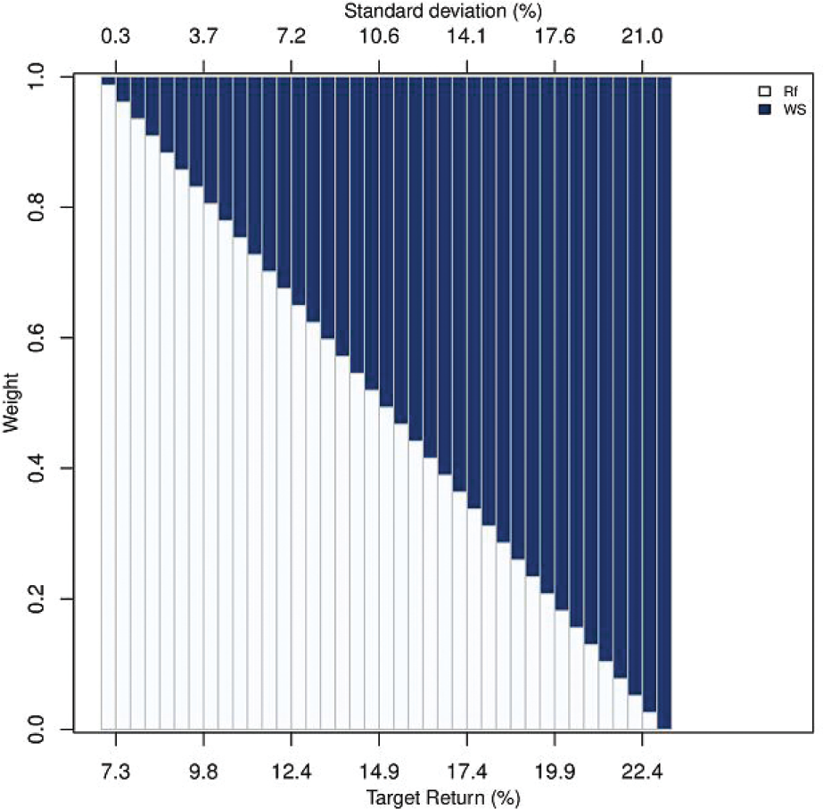
It is also interesting to look at factor investing, using only long portfolios (no short positions). Apart from the risk-free asset and the market portfolio, there are 10 sub-portfolios (6 combinations of size and value, and 4 combinations of size and momentum). In the factor computations, 5 of these sub-portfolios are held long and 5 are held short, but in this exercise, we consider all these portfolios as long positions. We compute efficient portfolios allowing allocations to any of the 10 sub-portfolios as well as to the risk-free asset and the market portfolios. Optimal portfolios (Figure 7) include only 2 of these 12 assets—the risk-free asset and a momentum portfolio (small winners). At low levels of risk, the risk-free asset dominates, while at modest and high levels of risk, the momentum portfolio dominates.
CONCLUSION
The results presented here indicate that factor investing using value and momentum is a viable investment strategy in India, but size does not perform well. This remains true, even if short positions are excluded, and only value and momentum tilts to the market portfolio are considered. Institutional investors and other large investors may be able to implement these tilts quite easily. However, it is harder for retail investors to adopt this style of investing. There may be a scope for making factor-based investing accessible to retail investors through mutual funds (or even exchange traded funds) that make these factors available at low cost.
We conclude with a brief discussion of various investment considerations and ‘caveats’ that must be taken into account while contemplating factor investing.
Market Efficiency and Behavioural Finance
We are agnostic on whether factor returns are attributable to systematic risk (as Fama and other proponents of the efficient market hypothesis would argue) or whether they are due to systematic errors (as behavioural finance might suggest). The authors are sympathetic to behavioural explanations (one of the authors teaches a course on behavioural finance), and the momentum factor in particular is hard to reconcile with market efficiency and risk-based explanations.
But for an investor, the debate on market efficiency is less important than it might appear. As is evident from the results, all of the factors experience large drawdowns which make factor investing risky for any investor with a finite investment horizon. Even if an investor is totally convinced that a factor has no systemic risk at all, investing in the factor is risk free, only over extremely long horizons. The investment consideration for investors with a finite investment horizon is, therefore, how much of drawdown risk they are willing to accept to earn a factor premium. This is awfully similar to an efficient market investor, trading-off risk premium against risk.
As Asness (2015) puts it:
I say “This strategy works.” I mean “in the cowardly statistician fashion.” It works two out of three years for a hundred years. We get small p-values, large t-statistics, if anyone likes those kind of numbers out there. We’re reasonably sure the average return is positive. It has horrible streaks within that of not working. If your car worked like this, you’d fire your mechanic, if it worked like I use that word.
Factor Investing and Indexation
Investing in a market capitalization weighted index is one important alternative to factor investing. We take the view that the market factor is just one of several factors that earn a premium. It is not even the factor with the largest premium or the least drawdown. An investor contemplating, taking market risk to earn the market premium, should give serious consideration to other factors as well.
Implementation Issues: Factor Indexes and Transaction Costs
We would like to clarify that we have not developed factor indexes as of now. Even our market factor is not an index designed for investing. Most index funds track an index of 30 stocks (Sensex) or 50 stocks (Nifty), while our market factor has a much larger number of stocks.
Our goal has been to measure the size and time-series characteristics of the factor premiums, and establish that some of these factors are potentially quite attractive to an investor. This data is valuable both to passive and active investors. For example, an active investor who focuses on fundamental analysis to pick stocks might consider imparting a value tilt to the portfolio, or might decide to use momentum to hedge the risk of the value tilt. On the other hand, a passive investor might simply choose one or more mutual funds that have a value tilt.
The actual implementation of factor-based investing would involve trading off comprehensiveness (diversification) against liquidity and transaction costs. Our results provide several reasons to believe that such an efficient implementation would deliver attractive results net of transaction costs:
The factor premiums are quite large.
We have already filtered out illiquid stocks in our analysis.
The factor that is most affected by illiquidity is the size factor (small stocks are generally illiquid), and this factor is not attractive in India anyway.
The factor that has high churn and is, therefore, more exposed to transaction costs is the momentum factor, and this factor works well even for large stocks (though it works better for small stocks).
Other than momentum, the other factors are rebalanced only annually reducing the churn.
Even long only portfolios involving momentum and value have attractive returns.
ANNEXURE 1
Methodology for Factor Construction in Indian Equity Markets
From the list of all the firms listed in Bombay Stock Exchange (BSE) covered in the CMIE Prowess database, we excluded all the firms that were traded on less than 50 days in a 12-months period, prior to the portfolio creation date in order to ensure that the portfolios used for estimation are investible. After applying this filter, the number of firms in different years is in the range of 1,500 to 3,000.
The Fama–French methodology involves a cross classification of stocks on two dimensions: size, measured by market capitalization, and value, measured by the ratio of book value per share to market price per share—B⁄M ratio. For the value breakpoints, we followed Fama and French (1993): the top 30 per cent stocks in terms of the B⁄M ratio were classified as value (V), the bottom 30 per cent as growth (G) and the remaining stocks as neutral (N). We defined big firms (B) as the top 10 per cent by market capitalization and classified the remaining firms as small firms (S). This choice reflects the highly skewed distribution of market capitalization and liquidity in the Indian stock market. Combining these two classifications gives us six portfolios: BV, BN, BG, SV, SN, SG, where for example, BV is the big value stocks. All these six portfolios are value weighted portfolios.
The size factor SMB is the simple average of three return differences: SG–BG, SN–BN and SV–BV, each of which is a difference between two portfolios that are matched in terms of value and differ only in size. Similarly, the value factor HML (high minus low) is defined as the simple average of two differences: SV–SG and BV–BG, each of which is a difference between two portfolios that are matched in terms of size and differ only in value. The HML factor is, thus, designed to capture the effect of value while being largely free of the influence of size.
To compute the momentum factor, at the end of each month t stocks are classified as winners (W) and losers (L) based on their 11-months returns from the end of month t-12 to t-1 (the top 30% were classified as W and the bottom 30% as L). The buy-and-hold returns for month t + 1 are calculated based on the earlier classification. Using the previously created size groups, four size-momentum portfolios: WS (small winners), WB (big winners), LB (big losers), and LS (small losers) were formed. The momentum factor WML (winners minus losers) was computed as the simple average of the differences in the returns of WS–LS and WB–LB. The WML factor was, thus, designed to capture the effect of momentum while being largely free of the influence of size.
Returns are inclusive of dividends. In accordance with standard practice, we have not accounted for transaction costs or bid-ask spreads in the computation of the factors and the underlying portfolios. These costs would vary depending on the trade execution strategies of different investors.
Subsequent to the publication of our working paper, the data series has been updated regularly with the help of the Centre for Monitoring Indian Economy (CMIE), which has implemented our methodology and provided us the updated data files on a regular basis.