
Abstract
Background:
In a network meta-analysis (NMA), multiple treatments can be compared simultaneously by aggregating pieces of evidence from direct as well as indirect treatment comparisons in different randomized controlled trials (RCTs). Conventional NMA are performed using a normal approximation approach and can be applied for arm-level binary outcome data as well. This study aimed to estimate the treatment effects within a Bayesian framework using a binomial likelihood for a multivariate NMA model.
Methods:
The dataset consists of 57 RCTs comparing the effect of ten pharmacological drugs and a placebo for acute bipolar mania in adults. The binary outcomes of interest were treatment response and all-cause dropouts measured three weeks from the baseline. Binomial distribution was adopted for the number of events and the probability of event occurrence modeled on the logit scale. Jeffrey’s Beta prior was considered for the heterogeneity and inconsistency of standard deviation (SD) parameters. Cholesky and spherical decomposition strategies were adopted for the between-study variance–covariance matrix. Deviance information criterion (DIC) indices were computed to determine the model fit. All results pertaining to Markov chain Monte Carlo simulations and all analyses were carried out in WinBUGS software.
Results:
The estimated common heterogeneity SDs were similar, and the DIC values did not provide any evidence for superiority between the two decomposition strategies. The correlation (95% credible interval) between the outcomes was estimated as −0.31 (−0.71, −0.02) and −0.37 (−0.73, −0.03) for the Cholesky and spherical decompositions, respectively. Gelman–Rubin convergence statistics were stable, and Monte Carlo errors for all the parameters were around 0.005. Overall, olanzapine, paliperidone, and quetiapine were both significantly more effective and acceptable than a placebo when both the study outcomes were considered simultaneously.
Conclusions:
The findings favoring olanzapine, paliperidone, and quetiapine possess an excellent concordance with the one adopted in clinical practice, and the Canadian Network for Mood and Anxiety Treatments and Royal Australian and New Zealand College of Psychiatrists guidelines recommend these as first-line drugs for treating bipolar disorder.
Randomized controlled trials (RCTs) compare new drugs with a placebo or a standard available drug but they lack the comparison against all other available interventions in the same study. Therefore, head-to-head comparisons are usually unavailable between all the competing interventions. Network meta-analysis (NMA) is recommended in such instances allowing multiple pairwise comparisons across several interventions while combining direct and indirect comparisons simultaneously. 1 Furthermore, an NMA provides summary estimates of relative treatment effects on various treatment comparisons. In addition, when there is a lack of direct evidence for treatment comparisons and undertaking a new RCT including all the competing treatments is infeasible, performing an NMA is cost-effective for clinical decision-making.
To account for the variation because of different sets of interventions or inconsistency in the model, Jackson et al. 2 adopted the arm-based analysis approach for the model introduced by White et al. 3 under the Bayesian setting. This approach can be used to determine the average treatment effects across all comparisons and designs. It also provides a valuable modeling framework by allowing sensitivity analyses to be performed using only one sensitivity parameter, the inconsistency variance. Furthermore, Jackson et al. 2 suggested that their model should only be utilized in large networks with the presence of a small unexplainable quantity of inconsistency.
Bayesian hierarchical models for NMA were initially conceptualized under consistency assumptions,4–6 extending the concept first proposed by Higgins and Whitehead. 7 Lu and Ades 8 adopted the separation strategy 9 for modeling the between-study variance–covariance matrix to specify prior distributions for correlations and standard deviations (SDs) separately. The authors used the spherical parameterization technique to generate a positive-definite correlation matrix. 10 Furthermore, NMA has been conceptualized from multivariate meta-analysis, and its methodology is still in a developing stage, although a considerable amount of advances have been made and published in recent years.11,12 Even though some attempts have been made to extend the NMA methodology to multiple outcome settings,13–18 modeling of binary outcomes has been less explored. 19
Bipolar disorder is a recurring mental illness with significant morbidity and mortality and is the 16th leading cause of years lost to disability worldwide. 20 The World Mental Health Survey Initiative reported a total lifetime prevalence estimate of 2.4% across bipolar I disorder, bipolar II disorder, and bipolar subtypes. 21 In the bipolar I category that affects about 1% of the general population, acute mania is a condition of abnormally and persistently elevated mood. 22 Patients are usually treated with mood stabilizers and atypical antipsychotics.21,22 These pharmacological interventions were shown to be individually effective than a placebo in a univariate model but a multivariate model has not been attempted. Cipriani et al. 23 evaluated the effects of 13 antimanic drugs in 68 RCTs using the Bayesian univariate model proposed by Lu and Ades.4,5 The models were supposed to quantify inconsistency using continuous outcome data but were unable to locate it in the network. Currently, the arm-based analysis approach, presented by Jackson et al., 2 can be used whenever arm-level binary outcome data are available. In addition, the model worked specifically within the Bayesian framework. Hence, the present study aimed to estimate and compare the treatment effects using univariate and multivariate Bayesian NMA models for two dichotomous outcomes of pharmacological interventions for treating acute bipolar mania (ABM) in adults.
Data
The present study used the dataset of the Cipriani et al. 23 that evaluated the effects of 13 antimanic drugs in 68 RCTs. As the current work used a multivariate model, 3 drugs—asenapine, gabapentin, and topiramate—and their corresponding 11 RCTs were excluded from the analysis, as both the study outcomes—treatment response and all-cause dropouts—were not reported for these 3 in the 11 RCTs. Therefore, the present study was restricted to 57 double-blinded RCTs comparing the effect of 10 pharmacological drugs or interventions and a placebo for treating ABM in adults. These drugs included mood stabilizers, antipsychotics, and antidepressants, which were compared against each other and with the placebo as monotherapy or add-on agents. Participants were aged 18 or older, of both sexes, and had a primary diagnosis of ABM. The ten pharmacological interventions included in the study were aripiprazole, haloperidol, quetiapine, ziprasidone, olanzapine, paliperidone, divalproex, carbamazepine, lithium, and lamotrigine. Aggregated data on the two outcome measures, namely treatment response and all-cause dropouts, were considered from all the included RCTs and defined as follows.
Treatment response: the number of patients who responded to treatment. Here, the response is defined as a ≥ 50% reduction in manic symptoms on mania rating scales.
All-cause dropouts: the number of participants who dropped out of the study for any reason before completion.
Both the study outcomes were measuredfrom baseline to week 3.
Complete details of the dataset are provided in Table 1. In total, there were 13,188 adult participants across 57 RCTs. Among them, 12 (21.1%) and 1 (1.8%) studies did not report response and the number of dropouts, respectively. Thirty-eight (66.7%) studies compared an active drug with a placebo.
Treatment Details in 57 RCTs
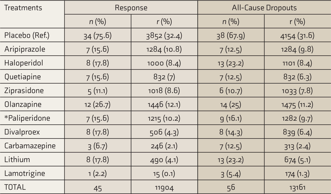
“*” paliperidone is the main active metabolite of risperidone. Data for these two drugs were combined.
n: number of trials, r: number of participants
Materials and Methods
An arm-based analysis approach 2 was adopted as data were available at the arm level for both dichotomous study outcomes. The arm-based analysis facilitates using an exact likelihood for the data rather than its normal approximation. For binary data, a binomial distribution can be adopted for the number of events and the logit scale to model the probability of event occurrence. 2 The models adopted for this study are described in the following sections.
Univariate Network Meta-Analysis Model
Let there are n RCTs comparing T treatments across all studies in an NMA. Let rtdi be the number of events for treatment t(I,j, …, T) in the ith study of design d, ntdi be the total number of patients in the tth treatment, and ptdi be the probability of event occurrence. Then, rtdi is distributed as
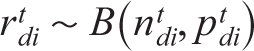
and
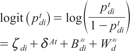
where
Assumptions of the model are as follows.
1. The study-specific arm-level parameters in the reference treatment arm are treated as fixed effects.
2. The heterogeneity variance is the same for all treatment comparisons across all studies, treated as random effects and defined as
where 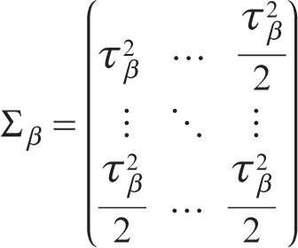
3. The inconsistency variance is the same for all treatment comparisons across all designs, treated as random effects and defined as
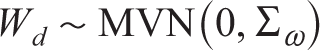
where 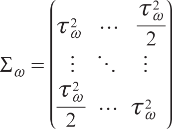
where MVN denotes the multivariate normal distribution.
This model is reduced to a consistency model (NMA-CM) when
In addition, the specification of the prior distribution plays an integral role in any Bayesian analysis. In the present study, normal (0, 100
2
) prior was used for the basic parameters
Jeffrey’s Beta Prior Distribution
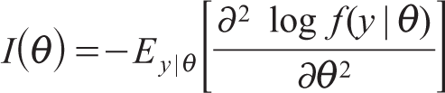
If p.d.f. of Y is 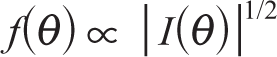
where Iθ is the expected Fisher’s information matrix and is defined as
Now, let us consider the binomial distribution with parameters n and θ, B (n, θ),
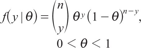
Then, Fisher information of θ is given by
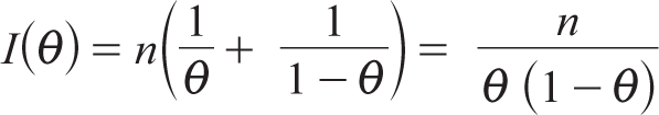
Thus, Jeffrey’s prior based on the binomial likelihood is
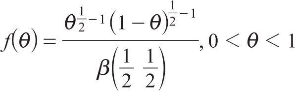
which follows the Beta distribution of the first kind, Beta (0.5, 0.5). Hence, the Beta distribution is a conjugate before the binomial likelihood, leading to a Beta posterior distribution. However, the advantage of Jeffrey’s Beta prior over uniform prior is that it is invariant under reparameterization. 25 In the present study, independent Beta (0.5, 0.5) prior distributions were used for the heterogeneity (τβ) and inconsistency (τω) SDs.
Multivariate Network Meta-Analysis Model
Estimation of the between-study variance–covariance matrix Σ β is important in a hierarchical multivariate model. As the present study intended to fit multivariate NMA-CM, Σ β plays a vital role. Different strategies to specify prior distributions for Σ β are discussed in the following sections.
Separation Strategies
The between-study variance–covariance matrix Σ
β
can be decomposed in terms of SDs and correlations,
9
allowing independent prior distributions for each of them. The decomposition of Σ
β
can be defined as
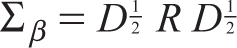
where
Separation by Cholesky Decomposition
In the Cholesky decomposition, the correlation matrix R is symmetric and positive semidefinite and can be factored as

where U is an upper-triangular matrix of order p × p. Diagonal elements of R are 1, and the off-diagonal elements must lie within the range [−1, 1]. Let the Cholesky factor 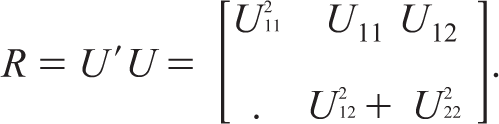
As diagonal elements of R are 1, we have U11 = 1 . The plausible intervals for other Cholesky factors can be derived and written as follows9,24:

where the uniform prior distribution is placed for U12 on this interval so that matrix R has correlations in the interval [−1, 1]. When the two study outcomes of the present study are negatively correlated, the uniform prior distribution on the Cholesky factor is taken with the interval [−1, 0].
Separation by Spherical Decomposition
A reparameterization of the Cholesky decomposition is the spherical decomposition wherein sine and cosine functions are used for 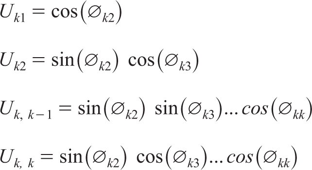
where 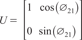
and the corresponding correlation matrix R is
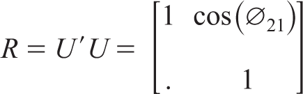
Assigning uniform prior distribution to the spherical factor
Ranking of Treatments
Under the Bayesian setting, to rank the treatments, at each iteration of the Markov chain Monte Carlo (MCMC), the largest (smallest) value of the basic parameters for the treatment response (all-cause dropouts) outcome is regarded as the most effective (acceptable). For the study outcome response (all-cause dropouts), if all basic parameters are of the positive (negative) sign, then the treatment is most effective (acceptable) than the placebo. The probability that treatments are most effective (acceptable) has been determined by the proportion of MCMC iterations in which they are the most effective (acceptable) and is treated as “probabilities of being the best treatment”. 2 The treatments can then be ranked based on their probabilities.
In the analysis, 16,00,000 MCMC iterations were included and thinning of 100 to reduce the autocorrelation in the sample. To ensure convergence, a 6,00,000 burn-in period was used, which was tested by running three chains with different starting values and using the Gelman–Rubin convergence statistic. Therefore, all estimates were based on 30,00,000 iterations, and the choice of these many iterations was to minimize the Monte Carlo (MC) error. Finally, the treatments were ranked based on their probabilities obtained through MCMC simulations. 2 All analyses were carried out in WinBUGS 1.4.3 software.
Results
Network plots were generated for both the study outcomes, i.e., treatment response [Figure 1(a)] and all-cause-dropouts [Figure 1(b)], to see the connectedness of the treatments.
Network Plots for the Outcomes. Response (a) and All-Cause Dropouts (b)
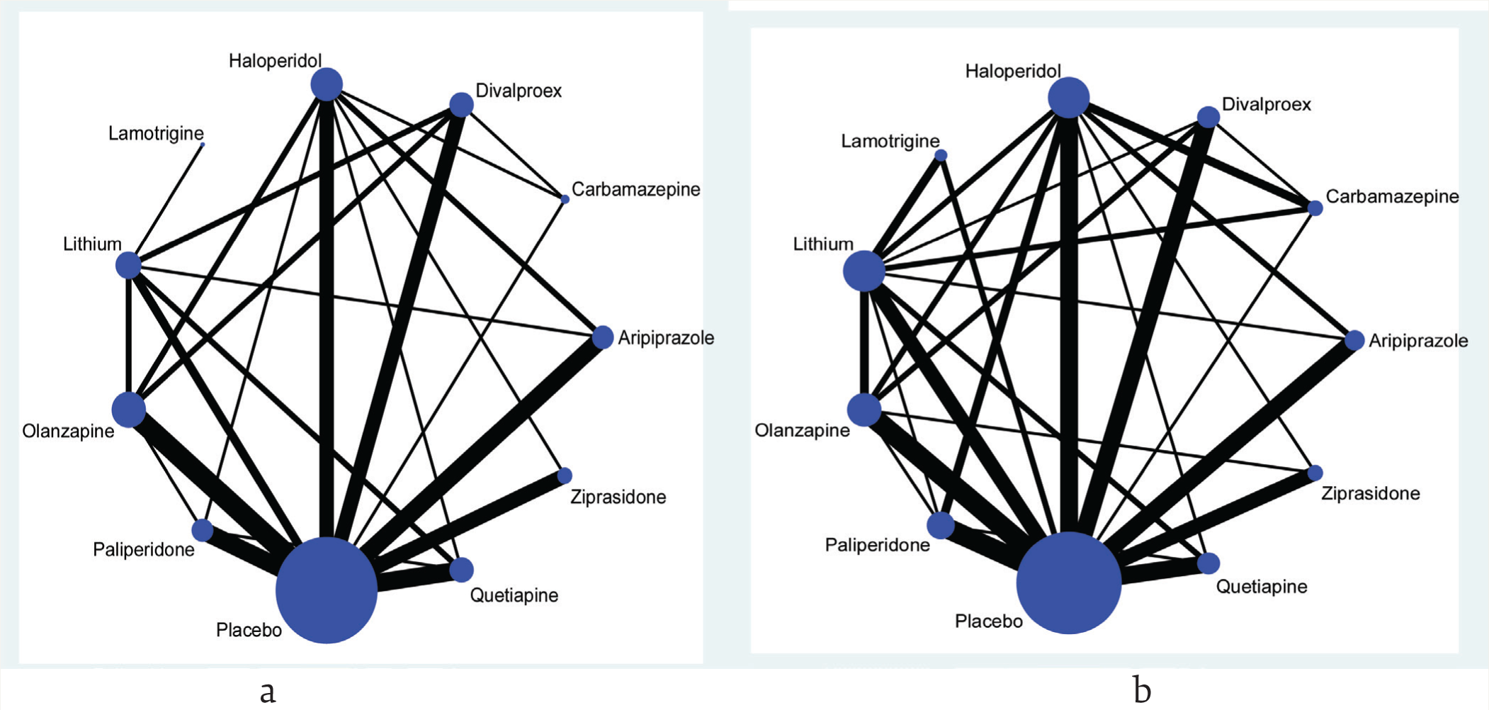
In a network plot, the node represents the treatments, and the size of the nodes reflects the total number of participants for that particular treatment across all the trials included in the analysis. The edge of the line connecting the two nodes represents a pairwise treatment comparison. Furthermore, the thickness of the edge represents the total number of trials in which the pairs of treatments have been compared. It is evident that the nodes are more well connected for all-cause dropouts than the treatment response.
Univariate Network Meta-Analysis
Response
In NMA-CM, the estimated posterior mean (95% CrI) of τβ was 0.29 (0.16, 0.43). Aripiprazole, haloperidol, quetiapine, olanzapine, paliperidone, divalproex, carbamazepine, and lithium were significantly more effective than the placebo, whereas ziprasidone and lamotrigine were not. Furthermore, carbamazepine has the highest probability (0.41) to be treated as the best, followed by paliperidone (0.19) and haloperidol (0.13). Similarly, in NMA-IM, the estimated posterior means (95% CrI) of τβ and τω were 0.28 (0.15, 0.43) and 0.07 (0.00, 0.25), respectively. The treatments that were significantly more effective than the placebo in NMA-CM were also significant in NMA-IM. However, carbamazepine remained the best (0.40) treatment in NMA-IM as well, followed by paliperidone (0.20) and haloperidol (0.13). The DIC values of both the NMA models indicated that the models were equally good (Table 2).
Univariate Bayesian Network Meta-Analysis Models for the Outcome Response
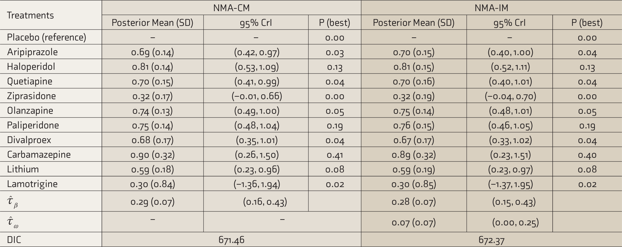
Estimates are in log scale, P (best): probability that each treatment is best, CrI: credible interval, SD: posterior standard deviation,
All-Cause Dropouts
In NMA-CM, the estimated posterior mean (95% CrI) of τβ was 0.40 (0.27, 0.54). Quetiapine, olanzapine, and paliperidone were significantly more acceptable than the placebo, whereas aripiprazole, haloperidol ziprasidone, divalproex, carbamazepine, and lithium were not. Lamotrigine was neither acceptable nor significant. Furthermore, paliperidone has the highest probability (0.28) to be considered the best, followed by olanzapine (0.26) and quetiapine (0.22). Similarly, in NMA-IM, the estimated posterior means (95% CrI) of τβ and τω were 0.39 (0.25, 0.54) and 0.09 (0.00, 0.32), respectively. The treatments that were significantly more acceptable than the placebo in NMA-CM were so in NMA-IM also. However, lamotrigine remained to be unacceptable and insignificant. Interestingly, both olanzapine (0.26) and paliperidone (0.26) have the highest probability to be treated as the best in NMA-IM, followed by quetiapine (0.23). The DIC values of both the NMA models indicated that the models were equally good (Table 3).
Univariate Bayesian Network Meta-Analysis Models for the Outcome of All-Cause Dropouts
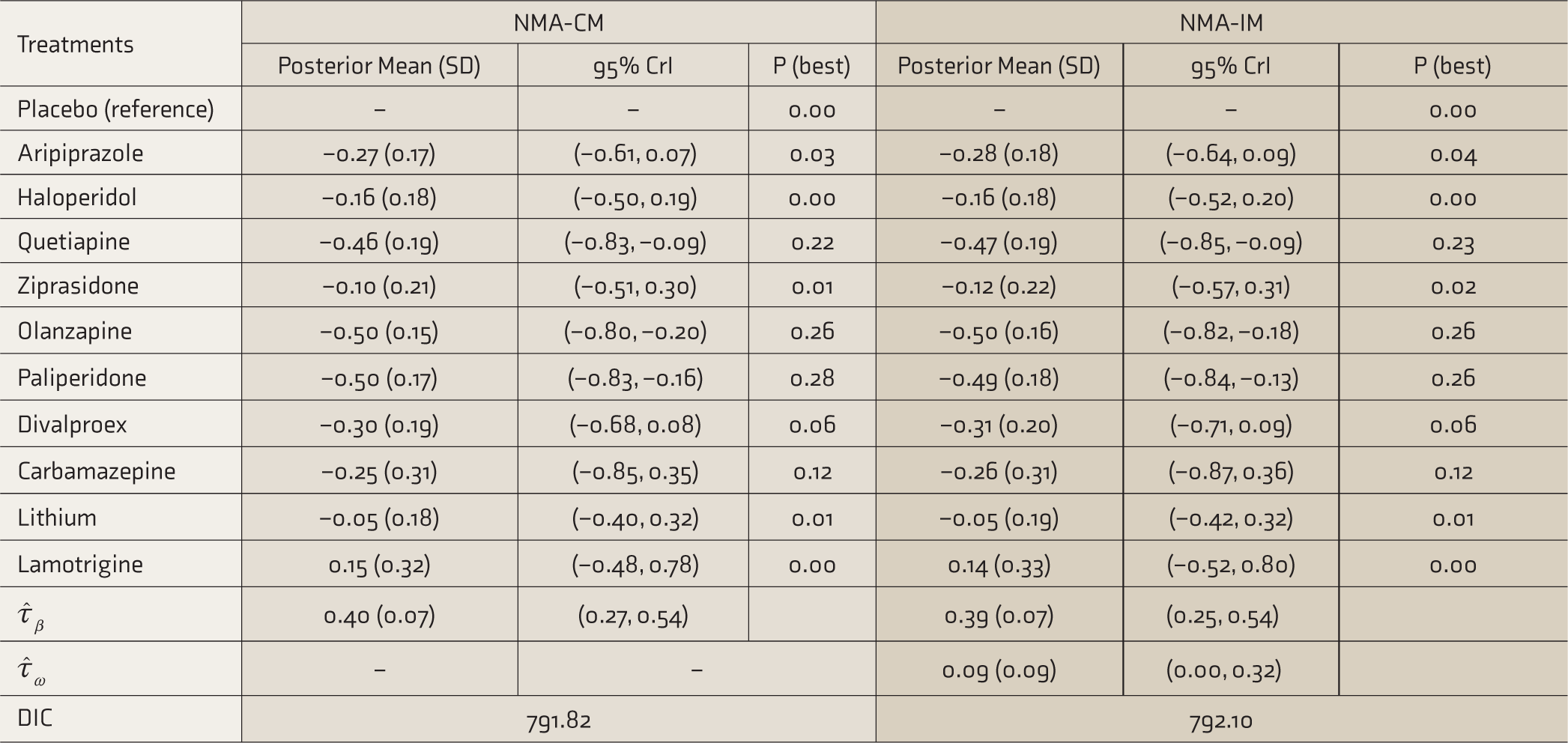
Estimates are in log scale; P (best): probability that each treatment is best, CrI: credible interval, SD: posterior standard deviation,
Multivariate Network Meta-Analysis
The between-study (heterogeneity) variance–covariance matrix Σβ was decomposed into the SD
Cholesky Decomposition
The estimated posterior means (95% CrI) of τβ for response and all-cause dropouts were 0.28 (0.14, 0.40) and 0.37 (0.26, 0.49), respectively. The correlation between the outcomes was estimated as −0.31 (−0.71, −0.02). Moreover, olanzapine, paliperidone, and quetiapine were significantly more effective and acceptable than the placebo, whereas aripiprazole, haloperidol, ziprasidone, divalproex, and carbamazepine were not. Furthermore, both lithium and lamotrigine failed to be effective and acceptable (Table 4).
Multivariate Bayesian Network Meta-Analysis Consistency Model Under Cholesky and Spherical Decompositions
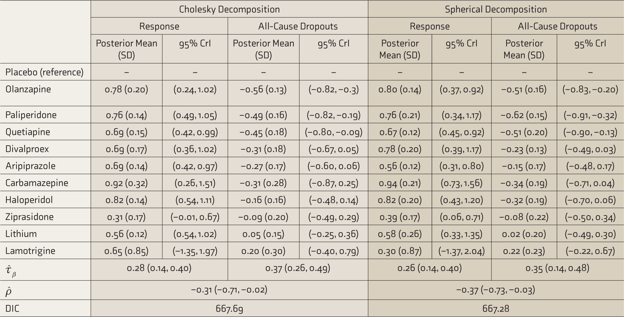
Estimates are in log scale, CrI: credible interval, SD: posterior standard deviation,
Spherical Decomposition
The estimated posterior means (95% CrI) of τβ for response and all-cause dropouts were 0.26 (0.14, 0.40) and 0.35 (0.14, 0.48), respectively. The correlation between the outcomes was estimated as −0.37 (−0.73, −0.03). Moreover, olanzapine, paliperidone, and quetiapine remained to be significantly more effective and acceptable than the placebo, whereas aripiprazole, haloperidol, ziprasidone, divalproex, and carbamazepine were not. Furthermore, both lithium and lamotrigine failed to be effective and acceptable. In addition, the DIC model fit index values for Cholesky (667.69) and spherical (667.28) decompositions were close to each other, indicating both decomposition strategies as equally good (
The Gelman–Rubin convergence statistics were stable for the prior distribution used, and all the MC errors were around 0.005. According to the trace plots, the stationary distributions were detected by the three chains as they drifted over the same region of the parameter space. However, the autocorrelation declined rapidly from lag 0 to lag 20; this suggested that each sample in the chain was slightly correlated with the preceding draws, signaling no autocorrelation and indicating no need for alarm. All these plots suggested that the samples are random and approximately independent. Kernel density plots were symmetric for the parameter estimate, implying that the chains converged to the same distribution. Overall, olanzapine, paliperidone, and quetiapine were both significantly more effective and acceptable than placebo when both the study outcomes were analyzed simultaneously.
Discussion
The present study compared 11 treatments, including 10 pharmacological drugs and a placebo, across 57 RCTs for treating ABM in adults. This study was restricted to two dichotomous outcomes, i.e., treatment response and all-cause dropouts, measured at three weeks from the baseline. Moreover, the current work is an extension of Cipriani et al.’s study 23 and the decision on the most effective pharmacological drug among the list of ten drugs in the present study was not only based on the univariate model but also supported by the results of the multivariate NMA model. Moreover, Cipriani et al. 23 used a contrast-based analysis approach, whereas we have framed the analysis under an arm-based approach. In addition, the Bayesian analysis in the present study allowed binomial likelihood in the model and also added the benefit of accounting uncertainty in the variance components while interpreting average treatment effects, which was not taken into account by Cipriani et al. 23
The two dichotomous outcomes were first analyzed independently using the univariate arm-based analysis within the Bayesian approach with Jeffrey’s Beta prior. Aripiprazole, haloperidol, quetiapine, olanzapine, paliperidone, divalproex, carbamazepine, and lithium were found to be significantly more effective than the placebo. On the other hand, for all-cause dropouts, quetiapine, olanzapine, and paliperidone were significantly more acceptable than the placebo. The results remained unchanged across the NMA models. Furthermore, for the outcome response, carbamazepine was found to have the largest probability to be the best across the NMA models; however, Cipriani et al. 23 showed haloperidol as the most efficacious drug. On the other hand, for all-cause dropouts, the ranking between olanzapine and paliperidone fluctuated between the NMA models. In terms of ranking between these two drugs, the most preferred drug remains undecided. Moreover, almost similar DIC values found in the study suggest that both the NMA models are equally good for both outcomes.
In practice, whenever multiple outcomes have been reported, it is more common to perform an independent meta-analysis for each outcome. In any study, multiple outcomes are recorded from the same subjects and are usually correlated. Ignoring it and performing a univariate meta-analysis for each correlated outcome may introduce bias and loss of precision. 28 They can be taken together in a multivariate model to explain the correlation between different outcomes at within- and between-study levels. As outcomes are recorded from each subject, there will be a correlation at the within-study level. Between-study correlation may exist because the true effects across studies depend on each other when measured in different situations. The application of multivariate meta-analysis is rare because of its complexity and lack of understanding. Riley et al. 28 highlighted the benefits of the inclusion of correlations in a model for the bivariate random-effects meta-analysis (REMA) over two separate univariate REMAs. Moreover, if missing at random is noticed for an outcome in some studies, the “borrowing of strength” will permit the bivariate REMA to produce noticeably smaller standard errors of the individual pooled estimates as compared with the univariate REMAs. 29 Utilization of correlation is referred to as “borrowing of strength,” which gives an advantage of using multivariate models over a univariate model. Riley et al. 29 used a simulation study to show that when some data are missing at random, the multivariate approach is likely to produce considerably lower standard errors and mean square errors of the pooled estimates than the univariate model, even when the study outcomes have moderate correlations. The authors also argued that given complete data, meta-analysts should not expect any gain in statistical efficiency over the univariate model; consequently, the standard error and mean square error of the pooled estimates are marginally smaller in the multivariate than in the univariate approach.
Furthermore, in addition to the results of the univariate approach, the results of the multivariate approach indicated that olanzapine, paliperidone, and quetiapine were significantly more effective and acceptable than the placebo when both the study outcomes were considered simultaneously in the multivariate NMA-CM. The estimated common heterogeneity SDs were similar between the two decomposition strategies. Noticeably, DIC values did not provide concrete evidence for preference between the decomposition strategies. Similar results were also obtained by Wei and Higgins, 24 who adopted both the decomposition strategies for acute stroke data framed under multivariate meta-analysis for four study outcomes and obtained almost identical estimated variance and DIC values. The authors used uniform (0, 2) prior distribution for the heterogeneity SD. A few studies had adopted the spherical decomposition framed under NMA with multiple outcomes on smoking cessation data 8 and prevention of poisoning injuries data. 19 To our knowledge, this is the first study to use both Cholesky and spherical decompositions in a multivariate NMA arm-based analysis strategy for binary outcomes. Also, the approach used in this paper does not require correlation to be known between the outcome variables. On the other hand, multivariate NMA-IM is yet to be developed; hence, only multivariate NMA-CM was investigated. This research points the way for further development of NMA-IM in a multivariate scenario.
Furthermore, the choice of the prior distribution for the heterogeneity and inconsistency SDs plays an integral role in a Bayesian NMA. The present study used Jeffrey’s Beta prior for the unknown SD toward statistical heterogeneity and inconsistency. However, the advantages of Jeffrey’s Beta prior over the uniform prior include the following: (a) it is reparameterization invariant 25 and (b) Beta distribution is a conjugate prior for the binomial likelihood that leads to a Beta posterior distribution.
Limitations
Apart from the strengths mentioned above, the current study possesses certain limitations worth acknowledging. First, the data used in this study were from 2011, 23 and new relevant RCTs completed after 2011 might have been missed. Consequently, it may be possible that some second-generation pharmacological drugs 21 for the treatment of ABM in adults were overlooked. Lastly, the treatments for ABM data were assessed based on how patients responded to the treatments and discontinuation for any reason before the end of the study. It would have been more informative to consider adverse events.
Future Directions
The present study used aggregated data, and it would be interesting for future research to focus on using both aggregated data as well as individual patient data. The present work’s scope was confined to estimating the treatment effects and the unknown variance components in a multivariate NMA model. In addition, it will be interesting to explore the properties of NMA methodology under various artificially generated and controlled modeling conditions through coverage, bias, and interval width estimates.
Conclusion
The present study highlighted the advantages of the multivariate NMA model over its univariate counterparts. It concluded that the three effective and acceptable pharmacological drugs identified can help clinicians in treating adults with ABM. These findings should be taken into account when developing clinical practice guidelines. Moreover, our findings have an excellent concordance with the one adopted in clinical practice. Olanzapine and quetiapine are the most commonly prescribed drugs for mania, and so is risperidone,21,23,26,30 of which paliperidone is a metabolite. All the major guidelines for bipolar disorder, including the Canadian Network for Mood and Anxiety Treatments guidelines 21 and the Royal Australian and New Zealand College of Psychiatrists guidelines,26,30 recommend these drugs as the first choice for bipolar disorder.
Footnotes
Declaration of Conflicting Interests
The authors declared no potential conflicts of interest with respect to the research, authorship, and/or publication of this article.
Funding
The authors received no financial support for the research, authorship, and/or publication of this article.