
Abstract
This paper addresses the important question of how governments set fuel excises. A theoretical framework leads seven possible nested hypotheses to explain fuel excise setting: (1) inflation adjustment, (2) fuel price relief, (3) coordination with GST revenue, (4) sterilisation of oil price shocks, (5) attenuation of the business cycle, (6) public debt financing, and (7) environmental action. Its reduced-form empirical counterpart is estimated with an asymmetric ARDL model with time-varying dynamics on quarterly data for Australia covering 1990 to 2023. It is found that all hypotheses but one are relevant in explaining policymaker’s actions, and their influence is quantified. Importantly, evidence suggests that business cycle and public finance are significant driving factors, each with asymmetric dynamics that depend on the direction of the shocks. These findings help understand the patterns observed in fuel taxation decisions and inform the evaluation and public discourse on the motives of fuel taxation.
1. Introduction
Automotive end users of fuel face two types of taxation in Australia: a federal excise levy that is set as a fixed amount of Australian dollars per litre and a Goods and Services Tax (GST) that is also set by the federal government. Unlike other jurisdictions such as the United States, Australian states do not impose additional fuel taxes. Since its formal introduction in 1929 coinciding with the commencement of domestic petroleum refining, the excise was hypothecated to road funding, meaning revenues were earmarked for infrastructure development. This link persisted until 1959, when fuel excise was reclassified as general revenue, severing its formal connection to road expenditure. 1 In 1983, the Australian government introduced indexation to Consumer Price Index (CPI) inflation to maintain the real excise revenue value. However, this was loosely followed and was not the only criterion for setting the fuel excise level. For instance, road financing needs were contemplated until 1992, when the link between the excise and road infrastructure budget was finally removed. In 2001, substantial excise cuts were introduced, following the introduction of the GST and the Global Financial Crisis. Indexation was formally abolished in 2001 but was claimed to be used as a main excise criterion (Cormann 2014). The recent downturn in the business cycle following the Covid-19 pandemic led to a temporary excise cut of 50 percent between 30 March and 28 September 2022 that official sources say it was directed to “relief households from high fuel prices” (Parliamentary Budget Office 2022).
Taken together, these policy developments suggest that fuel excise decisions have been shaped by a range of considerations rather than a consistent, rule-based framework. Overall, the “formula” that the Australian government has used from the 1990s to set fuel excise taxes is anything but clear. Empirical evidence strongly rejects CPI indexation as the primary mechanism for excise adjustment. As illustrated in Figure A1, the real excise value, defined as the nominal excise adjusted for inflation, is clearly not constant over time. If maintaining a constant real excise were the sole policy objective, the series would be expected to exhibit stationarity. However, the unit root test results presented in Table A2 confirmed its non-stationarity (non-mean-reverting) property.
Further insight into the intricacy of the issue can be obtained from Figure 1, which shows a breakdown of the nominal prices of unleaded regular gasoline and diesel fuel that are compared to the CPI evolution. The price breakdown includes a cost and margin component, which is essentially the pump price net of GST and excise. There is no indication that the excise adjusts to keep real fuel prices constant, although their influence cannot be discarded. Moreover, domestic fuel prices bear little resemblance to international oil prices and macroeconomic indicators in Figure A1, complicating any visual inference of policy drivers. Overall, these observations underscore the limitations of graphical and descriptive analysis and highlight the need for a well-defined multi-factor econometric framework to systematically examine the excise setting decisions.
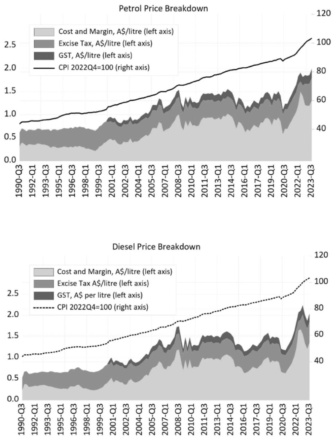
Breakdown of nominal gasoline and diesel prices in Australia.
The objective of this paper is to examine how different factors affect the fuel excise, leading to the following questions: How do governments determine fuel excise levies? Are excise adjustments primarily driven by inflation loss compensation? Are changes to real excise values mean-reverting? Are international oil price shocks considered? Are levies affected by the business cycle? Is fuel taxation used to finance public deficits? Are policy responses to different cyclical stages of output, fiscal accounts, and oil prices asymmetric? To answer the above questions, we develop a theoretical framework that yields testable nested hypotheses in a reduced-form empirical model. To our knowledge, this is the first attempt to formally lay out these important questions in a compact and testable model.
A straightforward approach to gain insight into the above would be to focus on the narrative of excise setting motives. However, such narratives may be ambiguous, incomplete, or strategically framed, making it difficult to discern the true drivers of excise policy decisions. To address this challenge, we propose a framework grounded in macroeconomic theory. Specifically, it is common in monetary analyses to use policy loss functions, rules hypotheses, and reaction functions to explain monetary authority decisions or optimal policies. In this paper, we postulate that the policymakers’ decisions are influenced by certain macroeconomic and energy market factors. Conceptually, it could be said that these factors enter a policymaker loss function alongside the fuel tax. An empirical model will measure how these factors affect fuel tax decisions, allowing the data to reveal the underlying policy mechanisms. This model shares similarities with the approach that Taylor (1993) introduced to measure monetary policy decisions. This loss-minimisation approach was refined in Rotemberg and Woodford (1997) and New-Keynesian models by incorporating households’ decisions as a constraint to obtain a closed model with rational expectations features. In our case, we treat macroeconomic variables as exogenous variables as changes in fuel taxes are typically small relative to the fuel price, causing limited impact on output given its price inelasticity and the small size of Australian oil production.
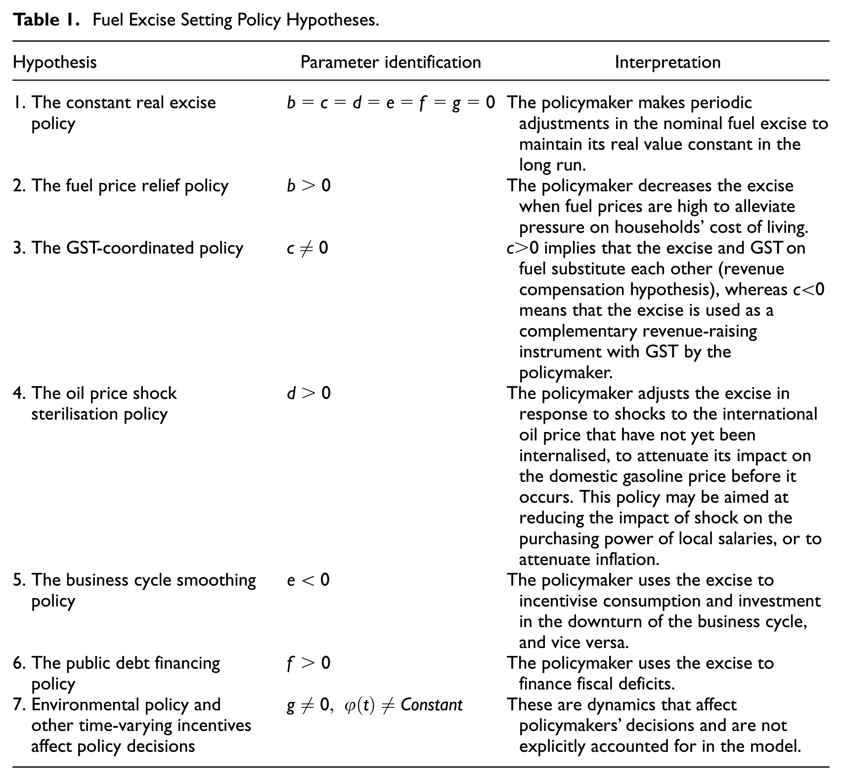
These theoretical considerations lead to seven non-mutually exclusive fuel excise setting hypotheses that are formulated from a policymaker’s perspective, namely, (1) inflation adjustment, (2) fuel price relief, (3) coordination with GST revenue, (4) sterilisation of oil price shocks, (5) attenuation of the business cycle, (6) public debt financing, and (7) environmental action. The empirical reduced-form model is tested with data for Australia covering 1990 to 2023. The findings support the existence of a long-run stable relationship that explains policy decisions. All the factors above are found to influence discretionary long-term excise-setting decisions, except for the international oil price. Importantly, it is confirmed that the business cycle and fiscal budget financing play a crucial role. Furthermore, the sign of the estimated coefficients of output gap and fiscal budget balance are found to cause asymmetric policy reactions. A final point to highlight is that the real excise exhibits non-mean-reverting dynamics that strongly associate with the way policymakers react to the business cycle. The results are supported by data for both unleaded gasoline and diesel.
The remainder of this paper is organised as follows. Section 2 reviews the relevant literature. Section 3 presents the theoretical and empirical model. Section 4 describes the data. Section 5 reports and discusses the empirical results. Section 6 concludes with policy implications.
2. Literature Review
Much of the literature on fuel taxation is primarily focused on their incidence, pass-through to fuel prices, role in fuel demand equations, and their relationship with international oil prices. Having said that, there is a small number of studies that have examined the determination of fuel taxes. Table A1 provides an overview of the literature summarising the time period, countries, methodology, and main results of the related studies.
A major strand of the literature is shaped by the rockets and feathers hypothesis that examines the asymmetrical link between oil and fuel prices, in which an increase in international oil prices has a greater impact on fuel prices than a same magnitude oil price reduction. This hypothesis has been verified with dynamic econometric models for the US (Bagnai and Mongeau Ospina 2018; Borenstein et al. 1997; Grasso and Manera 2007; Noel 2009, 2015; Sun et al. 2019), Europe (Bajo-Buenestado 2016; Karagiannis et al. 2015; Kristoufek and Lunackova 2015), and in multi-country studies (Apergis and Vouzavalis 2018; Kpodar and Abdallah 2017; Polemis and Fotis 2014). Deeper research into the causes of this unbalanced response is provided in Kaufmann and Laskowski (2005), Kaufmann et al. (2009), and Oladunjoye (2008) who largely attribute it to utilisation rates of refineries, inventories, and market structure.
Several studies have confirmed that the pass-through between fuel taxes and fuel prices is near-complete in the short-run (e.g., Ahundjanov and Noel 2021; Bello and Contín-Pilart 2012; Marion and Muehlegger 2011; Silvia and Taylor 2016). This result is consistent with price-inelastic oil demand and supply (upstream and downstream) constraints. Despite these findings on full tax pass-throughs, some studies have identified asymmetries in tax pass-through, whereby the proportion of a tax change passed on to consumers is greater when taxes are increased than when they are reduced (Doyle and Samphantharak 2008; Yilmazkuday 2017). Authors generally attribute this asymmetric effect to utilisation rates of refineries, transportation and storage in the supply chain, in line with the linkage between the oil price and fuel price. An important implication of a full tax pass-through, noted in Marion and Muehlegger (2011, 1211), is that the benefits of a fuel tax holiday is likely to accrue to consumers. For example, an unprecedented number of temporary tax breaks were implemented in Europe during 2021 to 2023 to lower fuel prices for consumers. Drolsbach et al. (2023) found that these measures were generally effective in reducing fuel prices with near-complete pass-throughs.
There is a relatively small literature on the determinants of fuel taxes. For example, Goel and Nelson (1999) found a negative relationship between gasoline prices and taxes, and Hammar et al. (2004) and Liddle and Lung (2015) found linkages between gasoline consumption and taxation. Highlighting the possible political considerations in diesel excise setting, Decker and Wohar (2007) found that diesel excise in the US was highly influenced by the trucking industry’s employment. Recognising that fuel taxation can generate significant revenue for the government, researchers have also found that government expenditure and/or debt is an important factor that drives fuel taxes (Chen et al. 2022; Hammar et al. 2004; Liddle and Lung 2015; Rietveld and van Woudenberg 2005).
While there are previous studies that considered public debt finances and tax coordination as determinants of fuel taxes, to the best of our knowledge, no study has assessed the setting of fuel taxes with an explicit and testable policymaker’s objective function. Moreover, the utilisation of fuel excise as an instrument to attenuate the adverse economic circumstances associated with Covid-19 in various markets is expected to attract renewed interest in the literature, addressing the same sort of questions examined here. This paper moves away from the estimation of pass-throughs to instead focus directly on the modelling of tax policy actions.
3. Theoretical Framework
To derive a dynamic theoretical model with testable hypotheses, we proceed with the specification of various dynamic components that are best explained in scaffolding blocks. It considers conjectural policymaker behaviours that are based on the discussions in Section 1 to build the hypotheses of interest, whose validity are tested on nested sub-models of an empirical reduced-form model.
The underpinning theoretical characterisation of fuel tax policy decisions in this paper can be derived from a policymaker’s loss function. The different factors affecting this decision could all be included in a single loss function. But it is also important to acknowledge that the actual tax decisions do not necessarily match what policymakers may consider optimal. This may be due to policy commitments and reputation considerations, which are captured separately. This can be written as:

where
A few observations can be made on how (1) is expanded throughout this section. First, real discretionary fuel tax changes are separated from real changes driven by inflation. Second, the set of fuel market variables include built-in constraints that will be substituted to obtain a reduced-form. Third, the macroeconomic conditions are assumed exogenous, which is suitable for Australia – a small producer and consumer of oil in the global economy. Being a price-taker in the global oil market, Australia may be subject to substantial aggregate supply shocks driven by changes in international oil prices affecting fuel prices, and the fuel tax changes are relatively insignificant. Given the inelasticity of fuel demand and supply, the impact on output and real activity variables can be considered negligible. The macroeconomic variables
3.1. Taxes, Prices, and Inflation
We start by distinguishing fuel excise levies, which are monetary charges per volumetric unit (litre), from the GST (also known as VAT in other countries) that is a percentage surcharge on the fuel price. The nominal value of the final fuel price,

where

It is important to distinguish between discretionary and non-discretionary tax policy interventions. A discretionary fuel tax policy intervention is an active decision by policymakers to purposefully modify the fuel tax component
Naturally, non-discretionary increases in tax revenue often occur without direct action by government authorities. For instance, an increase in the pre-tax fuel price, driven either by domestic conditions or the international oil price, would result in higher GST revenue. This happened repeatedly in the sample, as shown in Figure 1. These non-discretionary monetary tax increases could lead to discretionary decreases in the excise, if the policy objective was to maintain the combined tax revenue in real terms. Additionally, not all the changes to the nominal excise
To better formulate the interaction of passive and active policy reactions, four stylised scenarios are proposed in Figure 2. This diagram incorporates four assumption sets of increasing complexity. In all cases, real currency values are plotted against time. In Case (a), we assume that
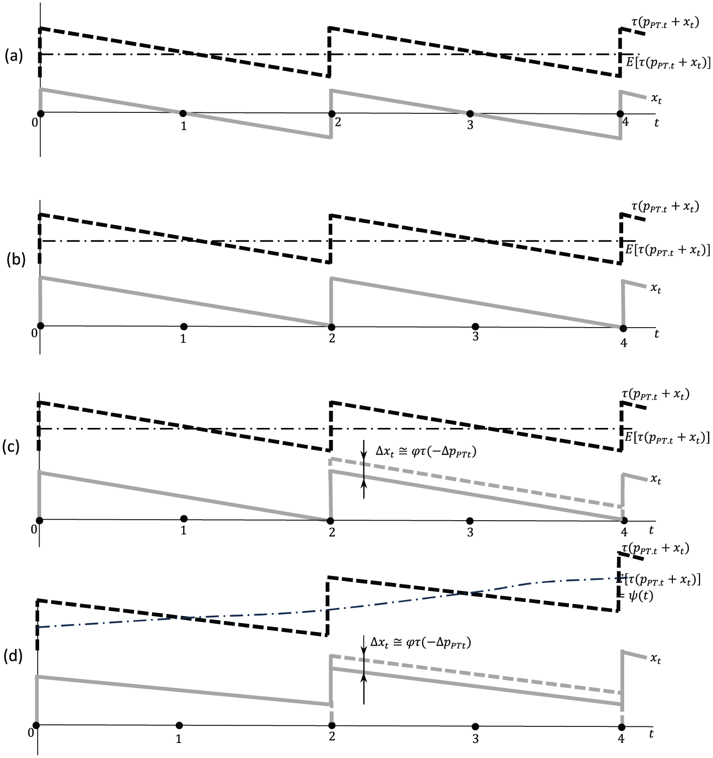
Excise change scenarios assume: (a) simple lagged inflation adjustment, (b) GST real revenue compensation, (c) reaction to fuel price shocks, and (d) arbitrary policymaker’s target.
3.2. Fuel Market Equilibrium Adjustment
The next step incorporates a market-clearing condition into the model and considers how it is affected by tax changes. Under perfect competition, a 1 dollar increase in the tax variable
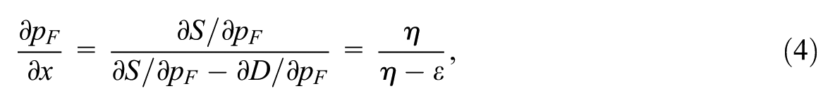
where
Combining (3) and all the assumptions introduced so far, it is possible to decompose a change in the real fuel excise value through the following difference equation:
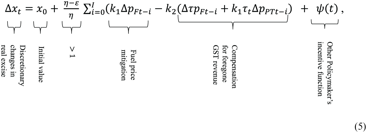
where
3.3. Macroeconomic Conditions
It was postulated that the policymaker minimises some policy loss function that depends, inter alia, on fiscal and macroeconomic performance, which are arguably two of the main reasons attributed to discretionary fuel excise adjustments. Fiscal needs are assessed with the fiscal budget balance variable

Following the authors’ recommendation for quarterly data, a weighting factor
3.4. Reduced-form Econometric Test
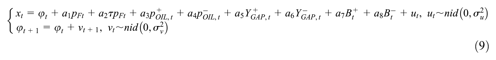
Equation (5) can be re-written as a cointegrated vector, that is, a linear combination of all variables in levels that is stationary over time. This vector can be interpreted as a long-run equilibrium relationship. The equation that explains
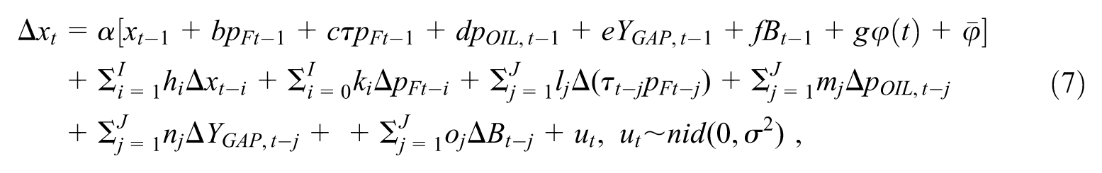
where
Fuel Excise Setting Policy Hypotheses.
3.5. Asymmetric Dynamics
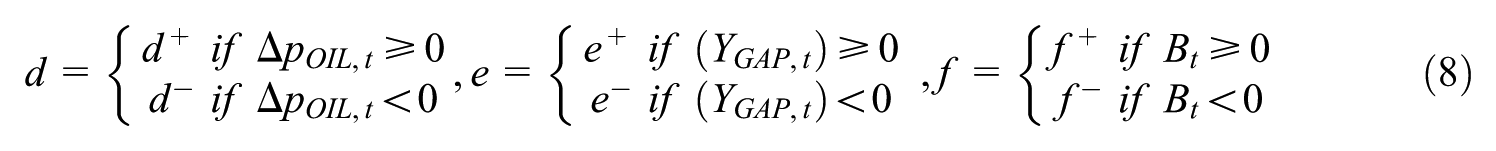
A widely used technique in error-correction modelling is the estimation of asymmetric loading factors, originally proposed by Granger and Lee (1989). This approach employs interaction dummy variables to estimate distinct coefficients for positive and negative changes in the independent variables. In the context of this study, it is particularly relevant to account for the possibility that policymakers may respond differently to positive versus negative output gaps, as well as to fiscal deficits compared to surpluses. In addition, several studies in the literature reviewed earlier suggest that oil price shocks may have asymmetric impacts on fuel prices. With these considerations in mind, the following asymmetries are incorporated in (7):
3.6. Hidden Dynamics in Fuel Tax Equation
In times series models, the Kalman filter procedure is often used to recover dynamic information that is not accounted for in the model. We apply this procedure to obtain in each period t, using information up to t, the recursive estimator
Note that from the above system, only
4. Data Overview
This study employs quarterly data spanning from 1990:Q3 to 2023:Q3, comprising time series measured either in real values (2022:Q4 Australian Dollars) or percentage changes. All variables have been seasonally adjusted. Fuel prices and tax data were sourced from IEA (2023). The end-user per-litre price of unleaded regular gasoline is denoted
Descriptive Statistics.
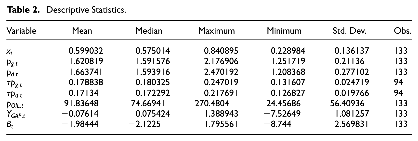
To proceed with the econometric implementation, it is important to consider the stationarity properties of the data. The ARDL cointegration method proposed by Pesaran and Shin (1999) and Pesaran et al. (2001) can accommodate time series having the same integration order or a mix of I(1) and I(0) variables, but not for variables that has a higher-order of integration (e.g., I(2)). Our unit root test results in Table A2 of the Appendix confirm the presence of a mix of I(1) processes (
5. Results and Analysis
The error-correction model in (7) was estimated with both gasoline and diesel data, and their comparison serves as a two-way robustness check. While an alternative approach could have involved constructing a representative fuel model based on a weighted average of gasoline and diesel prices, we opt for a more transparent approach that evaluates dataset implications separately to detect any potential model inconsistencies. This choice was further justified by the absence of reliable consumption data needed to construct appropriate weights. Notably, the results obtained from the gasoline and diesel models are highly consistent, suggesting that a weighted average model would likely yield similar conclusions.
Following Pesaran and Shin (1999) and Pesaran et al. (2001), the procedure commences by estimating an ARDL model with all variables in levels to apply the cointegration bounds test. If cointegration is found, this model is then re-parameterised into its error-correction representation. In order to correctly identify a parsimonious ARDL model, an identification procedure that uses the Akaike Information Criterion was implemented on an array of models in which each variable was allowed an independent lag structure. A total of 15,625,000 models were trialled to identify the baseline ARDL models for the gasoline and diesel markets.
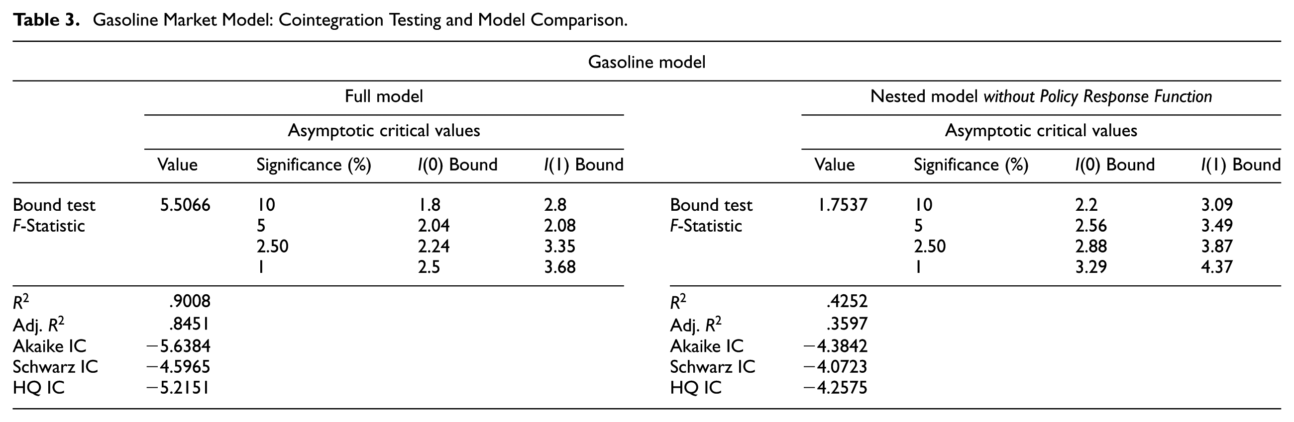
Tables 3 and 4 report the cointegration bounds test results. For both the gasoline and diesel models, the null hypothesis of no cointegration is strongly rejected at the 1% significance level, indicating the presence of a long-run equilibrium relationship. In addition, these models explain the excise variable considerably well, with values of
Gasoline Market Model: Cointegration Testing and Model Comparison.
Diesel Market Model: Cointegration Testing and Model Comparison.

The main estimations of the error-correction term in (7) are reported in Table 5.
3
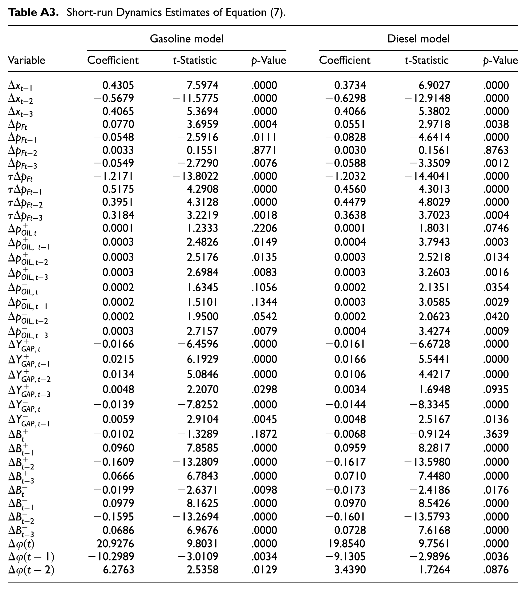
The models were estimated with an OLS procedure that verified all the standard assumptions of n.i.d. residuals. Two important data preparation steps took place before estimating these models. First, to capture asymmetric responses, positive and negative values of the output gap and budget balance variables were separated by sign-indicating dummy variables. For the international oil price, asymmetry was defined based on the direction of its change. Figure A1 provides a graphical account of when these changes occur. Second, the time-varying factor
Estimation Results of the Error-correction Term of Equation (7).
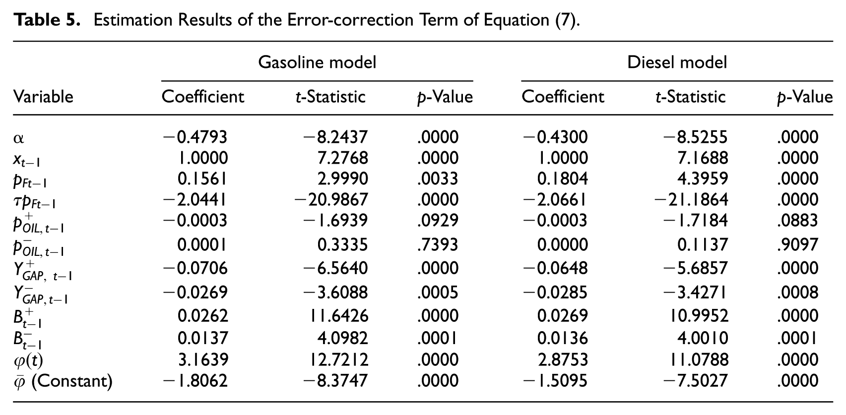
Table 5 verifies that the coefficient signs in the error-correction term satisfy the adjustment expectations. The independent variables in both models associated with the error-correction term have coefficient estimates that are significant at the 1% level, except for the oil price. This allows for validation of all the theoretical hypotheses except the one associated with the influence of the oil price. Specifically, the oil price does not appear to exert a significant effect during periods of decline, and its impact is only marginally significant during upward movements. It is worth noting that the coefficients associated with the oil price in this model are capturing oil shocks that have not been passed to domestic fuel prices. This finding suggests that policymakers do not consider oil price shocks that are not internalised by the market – typically those perceived to be temporary rather than permanent in nature. With respect to changes in the domestic fuel price, the coefficient estimates of
Turning to the GST revenue raised from fuel consumption, both models indicate that the estimated coefficient for
A noteworthy finding is the way fuel excise policy responds to the business cycle. In both models, real excise is found to be positively related to the output gap, consistent with the expectation that real excise is reduced during periods of economic contraction and increased during expansions. Quantitatively, a 1% increase in a positive (expansionary) output gap will lead to a 0.07% increase in the fuel excise, which is more than twice as large as the impact when the economy is experiencing a negative (recessionary) output gap. This asymmetry implies a lack of intertemporal compensation and suggests a cumulative upward drift in the real excise over time. From a distributional perspective, such dynamics may be perceived as inequitable to consumers, particularly if the excise burden disproportionately affects lower-income households.
An alternative interpretation of the asymmetric response of fuel excise to the business cycle warrants consideration. While the underlying rationale for this asymmetry may be multifaceted, one plausible explanation is that policymakers employ this mechanism to advance environmental agendas more aggressively during periods of economic expansion. Other interpretations include strategic cross-substitution between different sources of tax revenue or a broader trend towards increased government participation in the economy. However, disentangling these competing explanations empirically is inherently challenging due to overlapping policy motivations and data limitations. Notwithstanding these complexities, the analysis reaffirms that the business cycle exerts a significant and systematic influence on real fuel excise decisions in Australia.
Moving to the role of government budget balance, the coefficient estimates of
Finally, we turn our attention to the time-varying factor. The best way to interpret the estimates
6. Conclusions and Policy Implications
This study advances the understanding of fuel excise policy by introducing a formal theoretical framework and an empirical identification strategy – an approach not previously undertaken in the literature. The model offers a rich variety of nested hypotheses that can explain fuel excise policy decisions. Empirical implementation of the model to Australian data demonstrates the model’s strong explanatory power, as evidenced by the minimal dynamic residual information recovered through recursive estimation. Six of the seven excise-setting hypotheses were supported by the estimation results. Specifically, fuel excises were not only adjusted to maintain real value in response to CPI inflation, but also in ways that were consistent with fuel price attenuation, coordination between excise and GST revenue, attenuation of the business cycle and financing of fiscal budget. There was no compelling evidence that the international oil price affected the fuel excise, except through domestic fuel price changes.
The most salient finding of the analysis is the central role of macroeconomic factors in fuel excise determination. Excluding these variables drastically reduces the model’s explanatory capacity. The fuel excise response proved to be asymmetrical in an interesting way: excise cuts triggered by negative output gap are proportionally half as large as the absolute value of excise hikes in periods of positive output gap. As a result, as the business cycle of Australia regains stability, we would expect long-run upwards pressure on the fuel excise, holding other factors constant. Some could judge these dynamics to be unfair to consumers, but they could also be interpreted as an aggressive environmental policy stance (this study does not reveal the origin of the asymmetric policy reactions to the business cycle, but it confirms their presence). As for the use of the fuel excise to finance fiscal deficits, our results also show asymmetric dynamics in a way that suggests there has been cautious and measured use of fuel excise to address fiscal imbalances.
As our results suggest a complementary nature between GST and fuel excise, it is imperative that policymakers evaluate their combined impact on household budgets, especially during inflationary periods. Considering the effects of fuel taxes on the final fuel prices when the pass-through rate is expected to be high, policymakers have to be cautious when relying on these taxes to generate revenues. As lower income households tend to spend a larger proportion of their income on fuels, a fuel tax hike will disproportionally disadvantage these households, worsening income inequality, and potentially negating the effect of other social aid policies. Moreover, ongoing improvements in vehicle fuel efficiency and the rising popularity of low-emissions vehicles (e.g., electric and plug-in hybrid vehicles) are expected to reduce the amount of fuel excise collected by the government. This trend suggests that fuel excise may become a less effective tool for policymakers to achieve macroeconomic objectives. Our finding that fiscal surpluses lead to excise reductions that are nearly twice as large in absolute terms compared to excise increases during fiscal deficits suggests a prudent approach to fuel excise policy during periods of fiscal stress. Policymakers are therefore advised to maintain this cautious stance and avoid excessive reliance on fuel excise during downturns, particularly considering its regressive nature and potential to suppress household consumption.
Although this paper is primarily motivated by observations on fuel taxation in Australia, the underlying dynamics are broadly applicable to other markets. Future research could explore the extent to which fuel excise decisions are shaped by similar factors in other countries. The modelling framework developed in this paper is readily adaptable to European countries, with only minor modifications required to account for institutional and policy differences. In contrast, application to the United States and Canada would necessitate more substantial adjustments, as state-specific fuel taxes are added to federal taxes in these jurisdictions. One limitation of the reduced-form model in this study is the implicit assumption that fuel demand and supply elasticities remain constant, which may not be compatible with large-scale replacement of internal combustion engine transportation with electric vehicles (something not yet observed in Australia). Future research may also incorporate time-varying price-elasticities explicitly into the model – something that is beyond the scope of this paper.
Footnotes
Appendix
Short-run Dynamics Estimates of Equation (7).
| Gasoline model | Diesel model | |||||
|---|---|---|---|---|---|---|
| Variable | Coefficient | t-Statistic | p-Value | Coefficient | t-Statistic | p-Value |
| 0.4305 | 7.5974 | .0000 | 0.3734 | 6.9027 | .0000 | |
| −0.5679 | −11.5775 | .0000 | −0.6298 | −12.9148 | .0000 | |
| 0.4065 | 5.3694 | .0000 | 0.4066 | 5.3802 | .0000 | |
| 0.0770 | 3.6959 | .0004 | 0.0551 | 2.9718 | .0038 | |
| −0.0548 | −2.5916 | .0111 | −0.0828 | −4.6414 | .0000 | |
| 0.0033 | 0.1551 | .8771 | 0.0030 | 0.1561 | .8763 | |
| −0.0549 | −2.7290 | .0076 | −0.0588 | −3.3509 | .0012 | |
| −1.2171 | −13.8022 | .0000 | −1.2032 | −14.4041 | .0000 | |
| 0.5175 | 4.2908 | .0000 | 0.4560 | 4.3013 | .0000 | |
| −0.3951 | −4.3128 | .0000 | −0.4479 | −4.8029 | .0000 | |
| 0.3184 | 3.2219 | .0018 | 0.3638 | 3.7023 | .0004 | |
| 0.0001 | 1.2333 | .2206 | 0.0001 | 1.8031 | .0746 | |
| 0.0003 | 2.4826 | .0149 | 0.0004 | 3.7943 | .0003 | |
| 0.0003 | 2.5176 | .0135 | 0.0003 | 2.5218 | .0134 | |
| 0.0003 | 2.6984 | .0083 | 0.0003 | 3.2603 | .0016 | |
| 0.0002 | 1.6345 | .1056 | 0.0002 | 2.1351 | .0354 | |
| 0.0002 | 1.5101 | .1344 | 0.0003 | 3.0585 | .0029 | |
| 0.0002 | 1.9500 | .0542 | 0.0002 | 2.0623 | .0420 | |
| 0.0003 | 2.7157 | .0079 | 0.0004 | 3.4274 | .0009 | |
| −0.0166 | −6.4596 | .0000 | −0.0161 | −6.6728 | .0000 | |
| 0.0215 | 6.1929 | .0000 | 0.0166 | 5.5441 | .0000 | |
| 0.0134 | 5.0846 | .0000 | 0.0106 | 4.4217 | .0000 | |
| 0.0048 | 2.2070 | .0298 | 0.0034 | 1.6948 | .0935 | |
| −0.0139 | −7.8252 | .0000 | −0.0144 | −8.3345 | .0000 | |
| 0.0059 | 2.9104 | .0045 | 0.0048 | 2.5167 | .0136 | |
| −0.0102 | −1.3289 | .1872 | −0.0068 | −0.9124 | .3639 | |
| 0.0960 | 7.8585 | .0000 | 0.0959 | 8.2817 | .0000 | |
| −0.1609 | −13.2809 | .0000 | −0.1617 | −13.5980 | .0000 | |
| 0.0666 | 6.7843 | .0000 | 0.0710 | 7.4480 | .0000 | |
| −0.0199 | −2.6371 | .0098 | −0.0173 | −2.4186 | .0176 | |
| 0.0979 | 8.1625 | .0000 | 0.0970 | 8.5426 | .0000 | |
| −0.1595 | −13.2694 | .0000 | −0.1601 | −13.5793 | .0000 | |
| 0.0686 | 6.9676 | .0000 | 0.0728 | 7.6168 | .0000 | |
| 20.9276 | 9.8031 | .0000 | 19.8540 | 9.7561 | .0000 | |
| −10.2989 | −3.0109 | .0034 | −9.1305 | −2.9896 | .0036 | |
| 6.2763 | 2.5358 | .0129 | 3.4390 | 1.7264 | .0876 | |
Funding
The authors received no financial support for the research, authorship, and/or publication of this article.
Declaration of Conflicting Interests
The authors declared no potential conflicts of interest with respect to the research, authorship, and/or publication of this article.
2
The Tapis crude oil price, produced in Malaysia and traded in Singapore, is the preferred benchmark for Australian fuels. Tapis price data was only available from 2011:Q2, so previous periods were proxied with the Brent crude oil price. A slope dummy variable to distinguish between the two sources proved non-significant.
3
The short-run dynamics of (7) are reported in Table A3 of the ![]() .
.