
Abstract
Increased CO2 in the atmosphere increases tropospheric temperatures, thereby changing other climate attributes. However, cutting CO2 emissions by reducing fossil fuel use raises concerns about economic development and energy security. Additional CO2 is also directly beneficial for plants. Adaptation measures are an alternative, but those that are public goods are unlikely to be efficiently deployed without explicit government action. A model is developed to illustrate some of these complex policy trade-offs. The analysis is simplified by focusing on CO2 accumulation in the atmosphere as a sufficient statistic for both the external effects of CO2 and the global transition from fossil fuels to alternative energy sources.
1. Introduction
Decades of attempts to prevent CO2 accumulating in the atmosphere have failed. Regressing the logarithm of annual average concentrations of CO2 at Mauna Loa against time, a decade at a time, reveals yearly growth rates of 0.46% from 1991 to 2000, 0.54% from 2001 to 2010, and 0.62% from 2011 to 2020. The failure can be traced to three problems.
The first is the global scope of the externality. Policies to limit CO2 accumulation require international cooperation, but each nation wants others to bear the costs of control.
Second, many benefits from CO2 emission control are delayed while the costs are immediate. As a practical matter, resource allocation decisions, whether made in the marketplace or via political mechanisms, tend to weigh short-term costs and benefits much more heavily than longer-term ones.
The third problem, which exacerbates the other two, is that fossil fuel combustion dominates both world energy supply and anthropogenic CO2 emissions. According to the EI Statistical Review of World Energy, fossil fuels provided over 82% of world primary energy consumption in 2021, while IPCC (2001) says that fossil fuel combustion accounts for around 75% of anthropogenic CO2 emissions. The link between energy use and CO2 emissions makes issues apart from climate change relevant to evaluating policy. Since energy enables a force to do work, it is an essential input to production. Affordable, reliable, controllable, storable, transportable, and versatile energy sources are indispensable to a modern lifestyle. Hence, governments are reluctant to implement policies widely understood to raise energy prices or reduce energy use, supply reliability, or convenience. The dependence of economic output on energy input and the use of oil products by modern armed forces also ties energy supply to national security.
Section 4 develops a model that formalizes these trade-offs. Since our focus is the connections between climate and energy policies, we ignore anthropogenic emissions of greenhouse gases other than CO2 and anthropogenic sources of CO2 apart from using fossil fuels to provide energy. The data cited above suggest that the simplification may also be reasonable. To motivate the modeling assumptions, Section 2 summarizes relevant scientific issues, while Section 3 outlines some critical economic considerations. Section 5 compares the model to the class of aggregated Integrated Assessment Models (IAMs), called “benefit-cost IAMs” by Weyant (2017). The model developed herein more closely resembles these IAMs than the more disaggregated models dubbed “detailed process IAMs” by Weyant.
2. Overview of Relevant Scientific Issues
CO2 is a colorless, odorless, non-toxic 1 gas that is directly beneficial to plants as an input into photosynthesis and hence essential for almost all life on earth. CO2 is also absorbed and released by oceans and the soil and, in the long term, sequestered in rocks and fossil fuels. The release of CO2 via fossil fuel combustion raises its concentration in the atmosphere. The rates of removal of CO2 by all sinks, including plants, then also increase, but not by enough to prevent the stock from accumulating at about one-half of one percent per year.
2.1. CO2 as a Greenhouse Gas
The harm from CO2 is indirect and depends on its stock in the atmosphere. CO2 absorbs and re-radiates some frequencies of infrared radiation emitted from the earth’s surface and atmosphere. Increased CO2 thereby impedes the transmission of long-wave radiation to space. Temperatures in the lower troposphere then must increase to balance incoming solar radiation not directly reflected to space by clouds, ice, and other highly reflective surfaces.
While interactions between individual gases and electromagnetic radiation are well understood, the altitudinal and latitudinal distributions of greenhouse gases alter the incremental effects of CO2. Both absorption and emission are temperature- and pressure-dependent, and radiation bands affected by greenhouse gases overlap, with those affected by CO2 already quite saturated. Despite the complexities, many researchers have concluded that the additional radiative forcing accompanying increased CO2 in the atmosphere can be approximated by a logarithmic function
2.2. Feedback Effects
Climate models incorporate feedbacks that reinforce the initial warming from increased CO2. The most important is that the initial warming increases evaporation and raises the amount of water vapor, the most significant greenhouse gas, in the Earth’s atmosphere. The modeled final effect from
2.3. Climate, Weather, and Temperatures
Adverse effects from CO2 accumulation arise partly from temperature increases in the atmosphere, on the land, and in the oceans. 4 Others are forecasted to arise from what is often called “climate change” as higher temperatures affect other meteorological phenomena. Climate is defined as the joint probability distribution of various meteorological measurements – such as temperature, rainfall, snowfall, humidity, frost-free days, hours of sunlight, cloudiness, and wind speed and direction – at a given location. Because of the substantial and predictable variation of these measurements within a year, the distributions are defined as functions of the ordinal day number within a year. A sample of multiple, traditionally thirty, years of observations is needed to measure climate. “Climate change” can then be defined as a change in the distributions of the meteorological measurements at one or more locations. There are several consequences of this definition.
First, climates constantly change from one 30-year period to the next since statistical measurements based on a sample size of thirty observations will have sampling variation. Imprecision in the measurements adds randomness. Equipment failures, poor siting, and other factors can also impart bias to measurements. An undetected change in the bias would also be measured as “climate change.”
Second, the phrase “climate change” often designates a change in “climate,” thought of as a singular object independent of location, occurring only as a result of human actions. It is often used even more narrowly to mean a change in “climate” (singular) only because of human emissions of greenhouse gases. In practice, humans affect climates (plural) in many other ways, including via urbanization, land clearance, introduction of invasive plants, and large-scale irrigation. 5 Climates also change independently of human actions. Volcanic eruptions have been shown to have short-run effects. Possible candidates for long-term natural forces that could affect temperatures and other climate attributes include long cycles in ocean currents and changes in the amount or distribution of incident solar radiation and other solar effects. 6 Some of these changes may affect climates by directly changing the type, geographic distribution, and amount of cloud cover.
Third, damaging weather events are often cited as the main threats from CO2. However, the occurrence of many of these events is consistent with the distributions of weather variables from decades prior to when CO2 accumulation could have had any significant effects. They are better characterized as extreme weather rather than climate change.
2.4. Measuring Harm from Changes in Climates
IAMs assume that harm from CO2 monotonically increases in the departure of globally-averaged surface temperature anomalies 7 (GSTA) from a base value. Different IAMs use different base values to measure damages. The chosen base value is rarely explicitly justified as “ideal,” but the pre-industrial (Little Ice Age) average would surely be too low. 8
Another important fact for climate policy is that changes in distributions of meteorological phenomena following an enhanced greenhouse effect will differ by location. Furthermore, the net costs of those changes will depend on location. In some regions, extreme hot or cold temperatures impact welfare most, while extreme rainfall, high winds, or droughts are most impactful in others. It would seem most unlikely that the same GSTA would be ideal for every location. 9
2.5. Direct External Effects of CO2
Increased CO2 accumulation also has direct external effects. Thousands of laboratory and open-air experiments have shown that CO2 enrichment increases plant growth and makes plants more tolerant of dryness by reducing transpiration (Pospisilova and Catsky 1999). Extra CO2 has already been shown to increase agricultural output. Costs are incurred to pump CO2 into commercial greenhouses to enhance productivity. More relevant for CO2 emission control policy, Taylor and Schlenker (2021) examined the effect of increased ambient CO2 on maize, soybean, and wheat yields in the main U.S. growing regions for these crops. They estimated a panel model of average yields at the county level with ambient CO2 concentrations measured by the NASA Orbiting Carbon Observatory-2 (OCO-2) satellite as the main explanatory variable. They also include measures of temperature, precipitation, criteria pollutants (CO, NO2, O3, PM10, SO2), and county fixed effects and time trends. 10 They summarize the results as implying that, independent of any climate impacts, a 1 ppm increase in CO2 increases yields for maize, soybean, and wheat by 0.5%, 0.6%, and 0.8%. Additional CO2 in the oceans should also assist phytoplankton growth, thereby enhancing marine ecosystem productivity more generally. 11
2.6. Natural Absorption of CO2
CO2 is absorbed not only by the growth of photosynthesizing organisms but also by other organisms exploiting that growth. In addition, oceans absorb more CO2 as its concentration in the atmosphere increases, although the interactions are affected by seawater temperature and alkalinity. National Oceanic and Atmospheric Administration (NOAA) Global Monitoring Laboratory (2022) has developed a model of global CO2 sources and sinks called CarbonTracker. They find that about half of anthropogenic CO2 emitted into the atmosphere is absorbed by natural sinks, but there are uncertainties associated with the underlying mechanisms and measurements. While the modeled mean annual increases in CO2 (in ppm/year) over 2000 to 2018 are close to the measured increases, the standard errors in the modeled annual increases are about the same magnitude as the measured increases.
3. Economic Issues Aaffecting CO2 Emission Policy
3.1. Marginal Damages
The potentially harmful effects of CO2 depend on the stock of CO2 in the atmosphere, which accumulates gradually. This has two implications for the marginal damage curve from CO2 emissions in any one year. First, the curve will have a positive intercept, as even trivial emissions that year will add to the existing harm and thus have a strictly positive effect. Second, the curve will be quite elastic as additional emissions in that year add only slightly to the damage from past and anticipated future emissions.
3.2. Marginal Costs of Emission Reduction
Emissions of conventional air pollutants (such as SO x , NO x , CO, mercury, or particulates) can be reduced in many ways. Changes in the production process or the type of fuel used can alter flue gas composition. Devices like precipitators, scrubbers, or catalytic converters can clean the pollutant from the flue gas before it is vented. Cutting output also will cut emissions at a cost of control equal to the forgone benefit from lost consumption minus the explicit (excluding the external costs) cost saving from reduced production. When many methods are available, emissions should be reduced using the lowest marginal cost method first. Once the marginal costs of different methods are equal, further emission reductions should use all those methods while keeping their marginal costs equal. This is known as the equimarginal principle. 12 It will give a function relating the minimum marginal cost of control to emissions.
3.2.1. CO2 as a Global Externality
The potentially harmful effects of CO2 depend on global emissions. The equimarginal principle then requires the marginal cost of emission reduction to be equal in all locations. In a world of sovereign nations with different resource endowments and goals, such an outcome will be difficult, if not impossible, to achieve in practice.
Most of the growth in CO2 emissions over coming decades is forecasted to come from large population developing countries. These forecasts are well-founded for several reasons. First, the large populations mean that a small increase in per capita energy use greatly increases total energy use. Second, the mechanization of agriculture, industrialization, and urbanization accompanying the early stages of rapid economic growth greatly increase the energy intensity of production. Third, in prioritizing economic growth, these countries have preferred fossil fuels. Not only are they more affordable than the alternatives. They are also more reliable, versatile, transportable, and storable.
Controlling CO2 emissions in developed countries alone could raise CO2 emissions growth in the short run. Many energy-intensive industries would move to exempt locations, where CO2 emissions per unit of energy used are often higher. International transportation of bulky commodities also may increase.
3.2.2. Initial Marginal Costs of Reducing CO2 Emissions
It is commonly assumed that the marginal costs of reducing emissions of air pollutants start at zero at the uncontrolled level. In the case of CO2, and using the notation in Section 4,
Focus first on the oil market, where transportation fuel is the largest demand component. Most OECD countries tax vehicle fuel more heavily than many other goods or services. Usually, a tax would leave the marginal benefits of consumption above the marginal costs of production, implying
Parry and Small give three arguments supporting fuel taxes apart from any effect on CO2 emissions. First, they are a “second best”
13
way of internalizing environmental externalities from local toxic pollutants.
14
Second, by raising driving costs, fuel taxes are a “second best”
15
way of reducing traffic congestion and accident externalities. Third, the relatively inelastic demand for fuel may reduce the efficiency losses from taxing it. Parry and Small find the congestion externality is the largest component of a “second-best optimal” tax, while the pollution component is the smallest (and would remain so even without the CO2 externality). They also find that the U.S. tax rate is about half the “optimal” rate, while the U.K. rate is about double it. U.S. fuel efficiency and other mandates – including emission tests for vehicle registration – partially address the pollution externality, while increasing use of road and bridge tolls, parking taxes, and public transport subsidies partially address the congestion one. In summary, these arguments suggest
Many oil-exporting countries subsidize oil products, which would normally cause the marginal cost of production to exceed the marginal benefits of consumption. However, many of the subsidizing countries are OPEC members restricting supply. Even the subsidized domestic price likely exceeds their relatively low marginal cost of production. Then
In the case of natural gas and coal, their main uses are as inputs into electricity generation, industrial processes (fertilizers, petrochemicals, and metallurgy), and space and water heating. Subsidies and anti-competitive behavior are less significant in these markets. In developed countries, environmental externalities from local toxic pollutants are largely internalized by anti-pollution devices installed due to regulations or as responses to taxes or tradable permit schemes. Coal combustion in many developing countries produces significant environmental externalities from local toxic pollutants. This would make
Summarizing,
3.2.3. Elasticity of Marginal Ccost
The marginal cost of controlling CO2 emissions will likely rise steeply as emissions decrease. Current technologies for removing CO2 from flue gases are more costly than comparable technologies for removing conventional pollutants. This may be partly the result of CO2 being a much larger constituent of the flue gases. 16 In addition, once the CO2 has been captured, it currently is costly to sequester in bulk. 17
Given current technologies, the marginal cost of reducing fossil fuel use will likely rise steeply. The low elasticity of energy demand implies that the foregone marginal benefit of reduced energy use will rise steeply. Instead, fossil fuels could be displaced by alternative energy sources that release less CO2 per unit of energy supplied. Pigouvian taxes or marketable CO2 emission permits could achieve reductions at minimum cost, but governments have instead relied on mandates and subsidies for electrifying transportation, industry, and space and water heating and for generating electricity using wind and solar. These policies have substantially increased energy costs while doing little to slow the growth in CO2 emissions. For example, Hartley (2018) examined the effect of taxes on natural gas in Texas. At moderate tax rates, the elasticity of the electricity cost with respect to the natural gas price was roughly 40 times the elasticity of emission reductions. 18
Wind and solar raise system-wide electricity costs for several reasons. The average load factor for wind farms is at best around one-third, and for utility-scale solar plants at best around one quarter, compared to over 90% for nuclear plants and up to 80% for coal plants operated to supply base load as intended. 19 Lower load factors and a shorter lifespan for wind and solar plants raise capital costs per MWh of electricity produced.
Long transmission lines are often needed to get the power from wind and solar plants to market. This is partly because the best resources are often distant from load centers. In addition, the low energy density of wind and solar energy means wind and solar plants require substantial land per MW of capacity and sites with lower land costs are also often distant from load centers. Transmission lines from renewable plants also tend to be used at low load factors, further increasing their costs per MWh supplied.
The wide range of realized wind and solar load factors, from 0% to above 90%, means that substantial backup capacity, often enough to meet the entire load, is needed to ensure system operation. A separate issue is that realized wind (and, to a lesser extent, solar) load factors dramatically fluctuate over brief intervals. As unanticipated blackouts are very costly, more quick-start generators are needed to keep voltage, frequency, and reactive power within fine tolerances. Grids where wind generators are even 20% of total capacity, but more significant locally because transmission capacity constrains electricity trades, have experienced reliability problems. Intermittent generation currently needs backup thermal capacity unless hydroelectricity based on stored water is available. 20 The thermal technologies with the lowest marginal costs are base load plants, but they are unsuitable for quick-start backup. Traditional nuclear plants are designed to operate at full capacity except when refueling, and it can be costly and hazardous, unless specifically allowed for, to quickly cycle them up and down (Lokhov 2011). Cycling baseload coal plants can increase SO x and NO x pollution because control equipment is tuned to operate when the plant runs at full capacity (Bentek Energy LLC 2010). Cycling any plants using steam turbines can waste energy as a head of steam is maintained without producing electricity output. As a result, open-cycle gas turbines, which have relatively high operating costs, are most often used to back up intermittent renewables. As backup plants are offloaded when wind and solar plants operate, they are used at reduced load factors, which increases capital and other fixed costs per unit of output. Rapid ramping of plants can also increase stress and raise maintenance costs.
Qvist and Brook (2015) argue that only nuclear power and hydroelectricity have proved capable of deeply cutting CO2 emissions by displacing fossil fuels. Hartley (2018) examined strategies for displacing fossil fuels in Texas and found that supplying the Texas 2016 load with wind and storage would be about 28% more expensive than using nuclear and storage. The explanation is that electricity storage is very costly, and because wind generation is intermittent and poorly correlated with load, it requires 96% more storage capacity. At a low CO2 tax rate, wind backed up with natural gas generation was less costly than nuclear with natural gas backup. However, even moderate increases in tax rates made nuclear with natural gas backup, and then nuclear with storage, less costly.
There is also doubt that mineral production could support a substantial displacement of fossil fuels by wind, solar, and batteries. According to a World Bank Report (Arrobas et al. 2017), wind and solar require about 30 times more copper than nuclear per MW of generating capacity, and wind 375 times more rare earths, 3 times more molybdenum, 2.3 times more nickel, and 1.8 times more chromium. Solar PV requires 90 times more tin, 80 times more cadmium, 60 times more lead, and 25 times more indium per MW of capacity than nuclear. The much lower load factors and much shorter life spans for wind and solar generators imply mineral requirements per unit of energy supplied would be far greater.
3.2.4. The Energy Security Externality
As discussed in Hartley (2017), reductions in the energy security of democracies could be another external cost of reducing fossil fuel use. If nations such as the US, Canada, Australia, and Norway reduce fossil fuel output, imports of fossil fuels from less dependable suppliers, like Russia and the Middle East, will rise. Furthermore, China dominates the production of many critical components or inputs for wind and solar plants. According to the International Energy Agency Photovoltaic Power Systems Program, in 2019, China accounted for 68% of global polysilicon production, 96% of global photovoltaic (PV) wafers production, 76% of PV cells production, and 71% of PV module production. The GWEC Global Wind Blade Supply Chain Update for 2020 ranks China as the largest producing country for wind turbines. Chinese firms, either as independents or OEMs for large international firms, control more than 50% of global wind blade production capacity. In a 2021 report, the U.S. International Trade Commission reported that China is now the leading exporter of wind-powered generating sets, accounting for about 10% of the market outside China. Finally, USGS data shows that China dominates production, especially refining, of many minerals critical to manufacturing wind turbines, solar PV, and batteries.
3.3. Alternatives to Emission Controls
Since CO2 is not directly harmful, reducing its accumulation in the atmosphere is not the only option for reducing damages. Actions classified as self-protection by Ehrlich and Becker (1972) can reduce the likelihood of harmful consequences from extreme weather. Other actions, classified as self-insurance by Ehrlich and Becker (1972), can lower the costs of adverse weather events after they have occurred.
Individuals and firms will take some insurance and/or protective actions in response to changing damages. For example, they may reduce heat stress by adopting air conditioning, improving insulation, or altering working conditions. Farmers may maintain agricultural output by increasing irrigation and changing crop types. Property owners may install sprinkler systems or change building materials to reduce damage from wildfires. These are termed “endogenous adaptation” in IAMs. Damages in those models assume that any efficient private self-protection and self-insurance measures are implemented.
Self-protection actions that are public goods require explicit policy to be efficiently deployed. Other actions may require changes in regulations or the elimination of subsidies to achieve an efficient outcome. Examples of such policies include: building dikes to protect vulnerable coasts; building levees, dredging rivers, and improving urban drainage; building dams, reservoirs and aqueducts to help protect against droughts, wildfires, and floods; undertaking controlled burns or building firebreaks on public land; mitigating urban heat island antecedents by changing zoning laws; removing subsidies to living on vulnerable flood plains or coasts or in areas subject to wildfires; planning evacuation procedures ahead of threatening weather events; training and equipping rescue services; improving weather forecasts to give better warnings to take precautions; changing building codes to increase structural integrity; and investing in research to develop crops more resilient to weather extremes. These measures can defend against extreme weather events within the natural range of variation in addition to shocks that result from a change in the distribution of weather due to either CO2 accumulation or natural forces.
Similarly, some self-insurance measures are public goods. Examples include better disaster relief (including improved cooperation between different jurisdictions), better policing to reduce criminal activities after disasters, improved coordination between emergency medical facilities, and improved civil reconstruction capability. Such measures can also reduce the costs of other disasters that have nothing to do with adverse weather events, such as earthquakes, tsunamis, volcanic eruptions, terrorist attacks, major industrial accidents, and pandemics. The fact that public self-insurance measures are useful in these other contexts raises their benefit/cost ratios.
Self-protection and self-insurance policies have several advantages relative to reducing CO2 emissions. They do not increase energy costs. Global agreement is not required to implement them, and each country can tailor measures to the risks they face. Any beneficial changes in weather resulting from increased CO2 can be retained. Finally, self-protection and self-insurance measures do not impinge on energy security.
4. Model
To limit the scope of the analysis, we ignore greenhouse gas emissions other than CO2 and anthropogenic sources of CO2 other than fossil fuel combustion. In addition, although intertemporal trade-offs make climate policy an optimal control problem, the model avoids that issue
21
by assuming that CO2 accumulation in the atmosphere is a sufficient statistic for both the external effects of CO2 and the comprehensive transition from fossil fuels to alternative energy sources. Specifically, the expected path of fossil fuel extraction cost is assumed to track cumulative fossil fuel use. Absent CCS (which, for simplicity,
22
we ignore), cumulative fossil fuel use also will determine the stock of CO2 that accumulates in the atmosphere. Use
The solid line in Figure 1 illustrates the expected path of fossil fuel extraction cost in the absence of climate policy. Serendipitous discoveries and new production technologies can temporarily increase the supply and/or reduce the costs of producing fossil fuels. Nevertheless, expanding demand for fossil fuels from large population developing countries (Section 3.2.1) will deplete lower-cost deposits, and raise the real prices of fossil fuel energy. For a given cost of alternative (or “backstop”) energy (initially taken to be exogenous), define
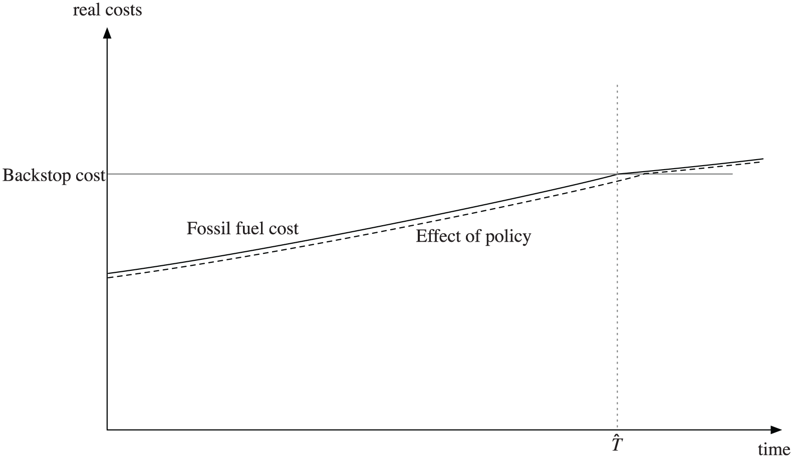
Expected path of fossil fuel extraction cost.
Climate policy, such as taxing CO2 emissions, reduces the CO2-intensity of GDP by encouraging fuel substitution or increased energy efficiency.
23
Policy implemented at
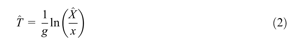
Based on a regression of the log of Mauna Loa annual average CO2 from 1959 to 2022 against time, we assume that

where
Using (1) and the observation that
The model thus incorporates a version of the “green paradox” 26 prevalent in optimal control models of energy transition whereby reductions in current fossil fuel use lower fossil fuel extraction costs and extend the time they dominate energy supply.
From sections 2.1 and 2.2, the impact of

where
Following Section 2.4, we assume that the costs of adverse weather events at

where
Let
Increases in
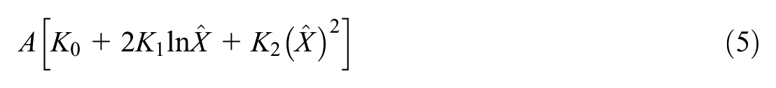
To convert expected damages (4), (5) and
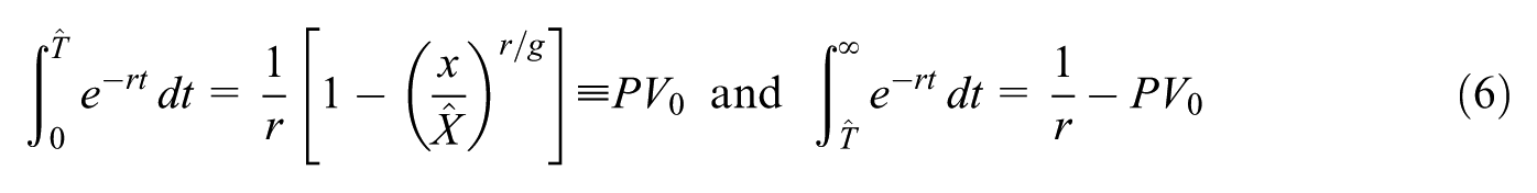
where we have used (2) to write
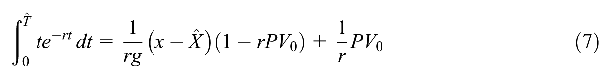
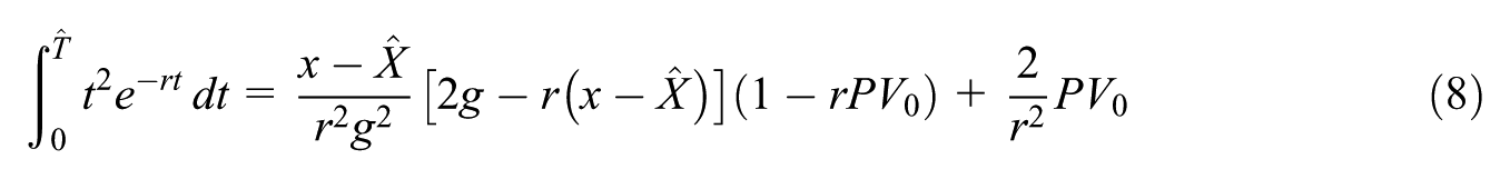
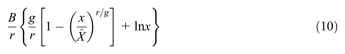
Using (6) to (8) with (4) and (5) the present value of expected damages can be written:
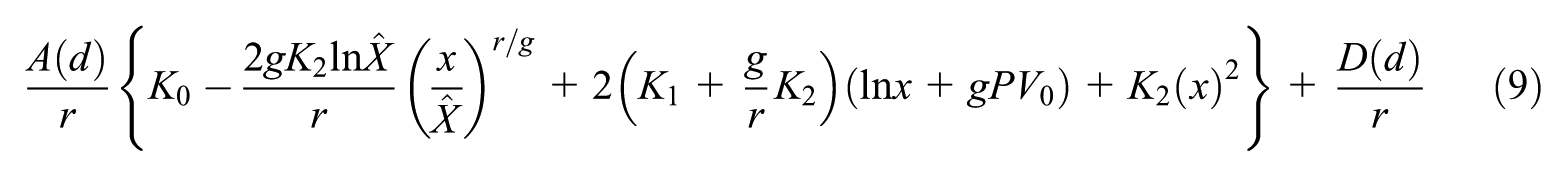
From Sections 2.5 and 3.2.4, increased fossil fuel use and atmospheric CO2 also provide direct positive external
31
net benefits. The marginal external benefits will likely decline as CO2 concentration increases. For simplicity, assume the welfare value of these external benefits as a fraction of GDP is proportional to
4.1. Global Model
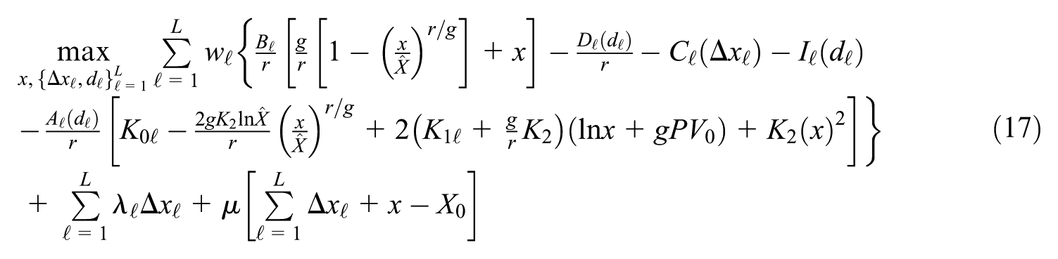
Optimal climate policy in a global model involves choosing
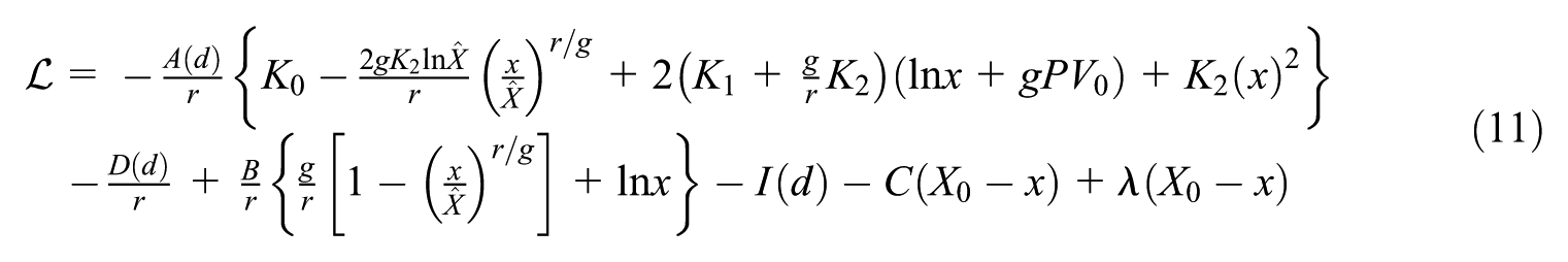
The first order necessary conditions for a maximum of (11) can be simplified to
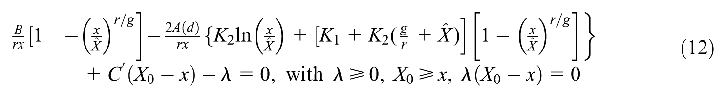

When

where
for
There is no need to allow for a
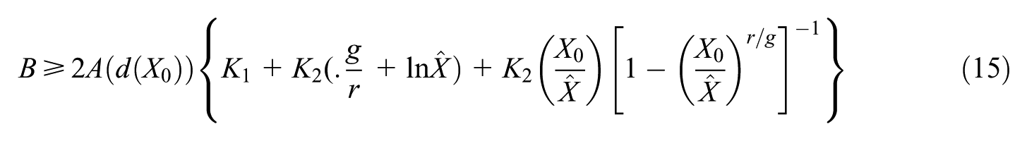
From (13), high
The bound on the right of (15) increases in
4.1.1. A Numerical Illustration of Solutions to (13) and (14)
Regressing the logarithm of the Manua Loa average annual CO2 level against time we find
To calibrate
Assume initially that
Equations (13) and (14) also involve the discount rate
Variables, Parameters, and Functions in the Numerical Example.
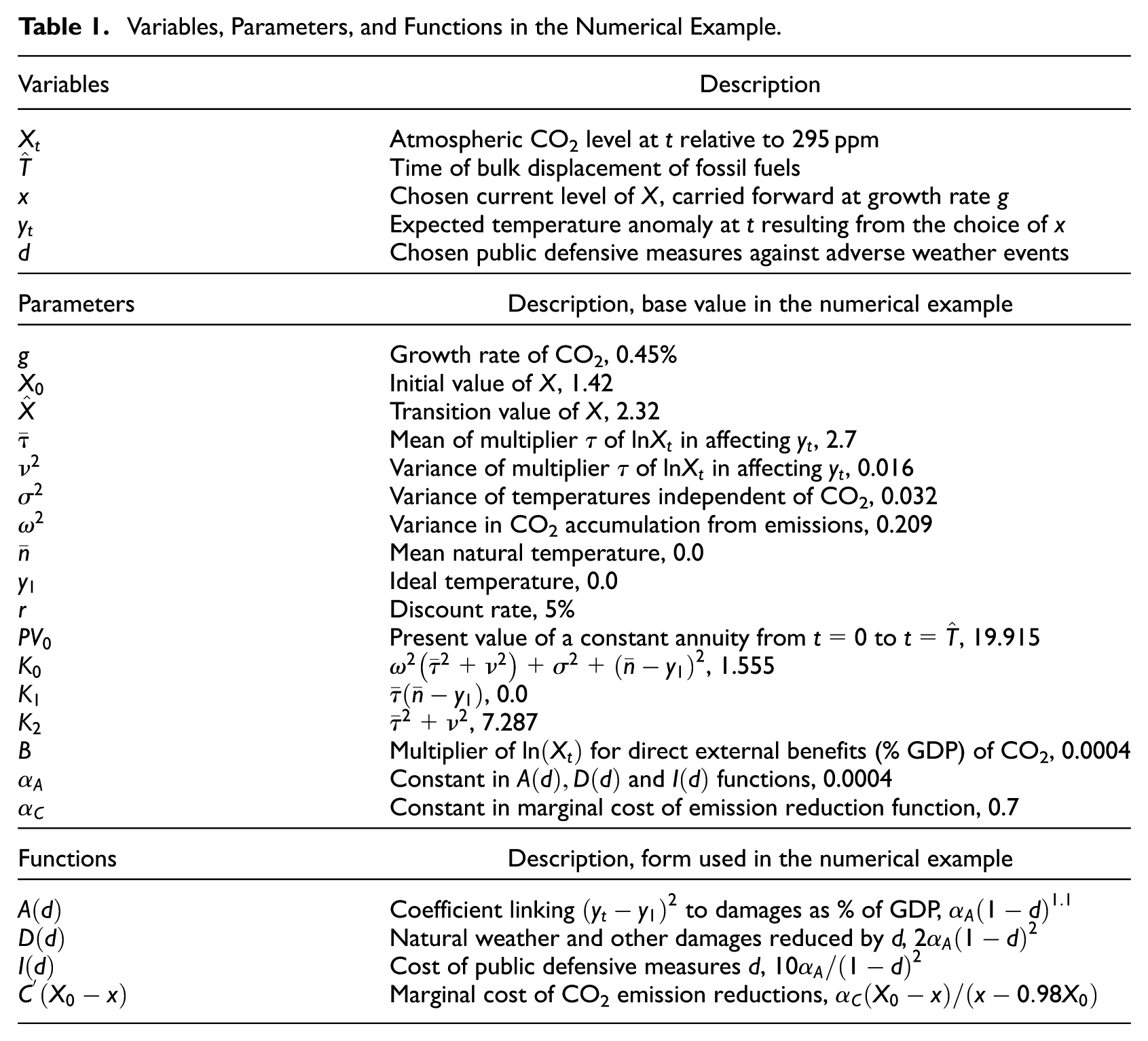
The functions
Equations (14) for
Since
We assume that the cost
IAMs typically define the cost of reducing CO2 as a function of emission reductions, whereas we need them as a function of reduced concentration of CO2 in the atmosphere. Using the estimated coefficient 0.525 relating emissions to concentration, average emissions over the last Fifteen years in the EI data of 4.13 ppm would change expected CO2 concentration measured as a ratio to 295 ppm by around 0.0074. We conclude, consistent with the arguments in Section 3.2.3 and the small effects of events such as the COVID lockdowns in 2020 and the 2008 financial crisis, that reducing
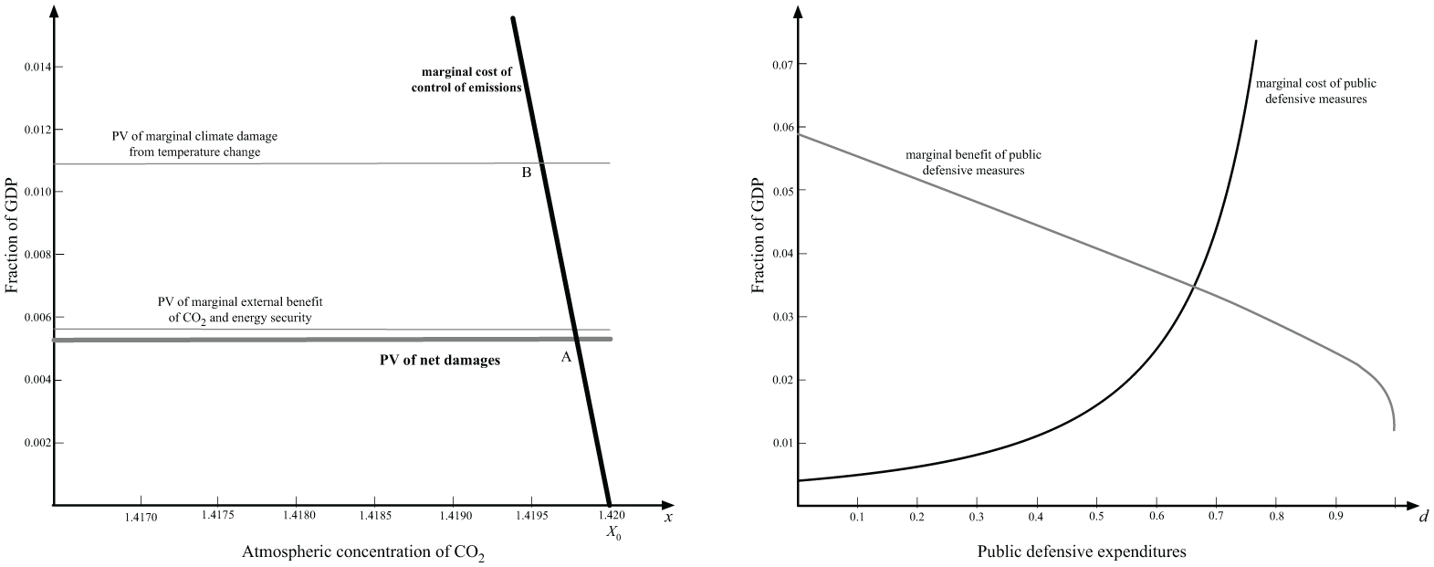
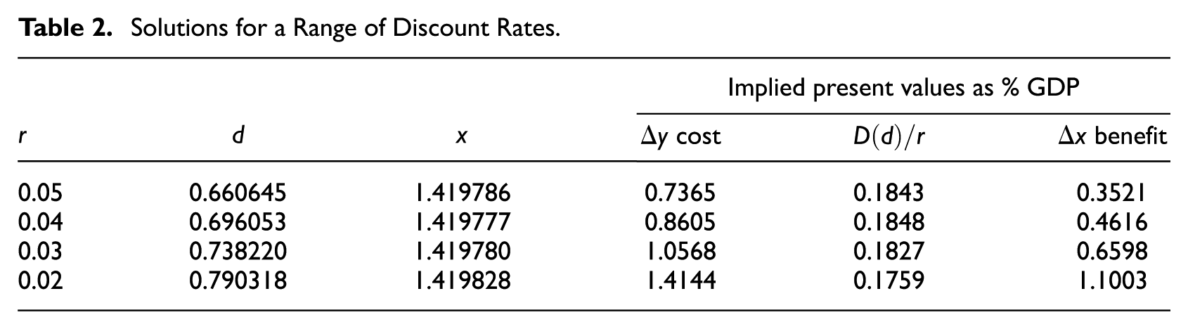
Figure 2 graphs equations (13) and (14) for the above functional forms and parameter values. The graph on the left illustrates the solution to (14) evaluated at the solution for
The additional elements in this model are the direct net benefits of CO2 represented by (10), the ability to reduce expected damages by spending on
Point B in the left graph of Figure 2 illustrates the solution for
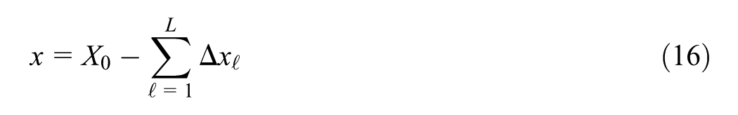
Reducing
Solutions for a Range of Discount Rates.
4.2. Allowing for Geographic Variations
Section 2.4 noted that higher temperatures could be less harmful or even beneficial in some locations. Introduce an index
4.2.1. Cooperative Solution
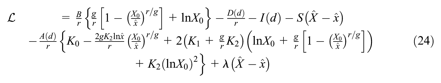
Under international cooperation, policies maximize a weighted sum of expected net benefits with
For
First order necessary conditions for the choice of public defensive measures
In the interior case, the first order necessary conditions for
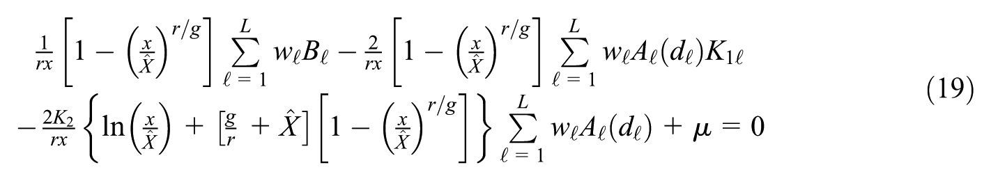

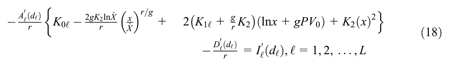
Combining (19) and (20) and using (18) gives
For
If (19) and (20) can be solved for
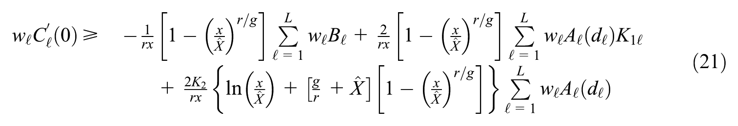
locations in the latter group will all have
The right side of (21) is identical across locations. If it is negative because, for example, at many locations
4.2.2. Non-cooperative Outcome
Now assume a Nash equilibrium where each government chooses its policies taking policies chosen elsewhere as given. Denoting the expected aggregate CO2 level
The first order necessary condition for an interior choice of
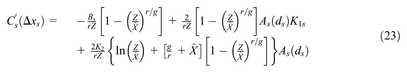
while the first order condition for
Comparing (23) to (19) and (20) clarifies the collective action problem for climate policy. Where (23) has
4.3. Technology Policy
Hastening the transition by subsidizing R&D into alternative energy technology could also reduce CO2 accumulation. To succeed, the policy must anticipate what alternative energy technology can displace fossil fuels en masse. A successful policy would lower energy costs starting from an earlier transition date, encouraging developing countries expected to dominate impending energy demand growth to adopt it voluntarily. Although the policy could be implemented without international cooperation, learning externalities could preclude an efficient outcome if such cooperation is absent.
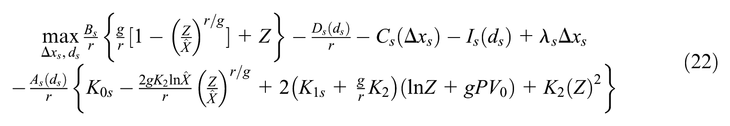
To investigate the policy, return to the simple global model but now assume that a subsidy with cost
The first order necessary conditions for

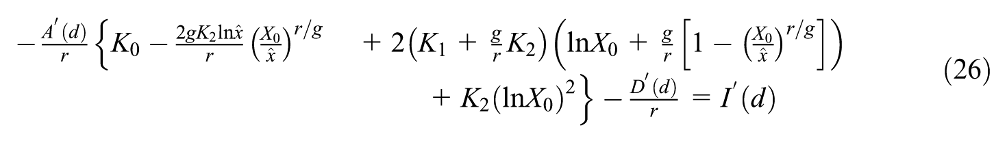
From (25), and noting that (26) becomes (13) with

The additional term multiplying
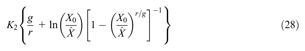
which is negative for
In the interior case for the choice of
for
5. Comparison to IAMs
Weyant (2017) notes that the main benefit-cost IAMs used to calculate optimal climate policies are the Dynamic Integrated Climate-Economy (DICE) model (Nordhaus 2014), the Framework for Uncertainty, Negotiation, and Distribution (FUND) model (Anthoff and Tol 2013), and the Policy Analysis of the Greenhouse Effect (PAGE) model (Hope 2011). He observes that the FUND model delivers the lowest net cost of CO2 emissions in part because it assumes a greater ability of those affected by climate change to adapt.
de Bruin et al. (2009) claim that most IAMs consider only induced (adjustment to the new climate represented in the model by transition costs and lags) and implicit (incorporated in the functional relationships) adaptation to climate change. Since these adaptations are of a “private nature,” they are assumed to be optimal and already incorporated into the damage function. de Bruin et al. (2009) modified the DICE model damage function to distinguish gross from net damages. The difference is the benefits of ecological, social, and economic changes in response to climate change minus the costs incurred. They find adaptation to be more important for reducing the costs of climate change in earlier periods, but mitigation becomes more important later.
In a more recent paper, Estrada et al. (2019) modified the damage function to make it a function not of the difference between GSTA and an unchanging base value but rather the difference between GSTA and an adjusting value
The distinction between autonomous and planned adaptation is partly related to the one we make between self-insurance measures (that lower costs ex-post) and self-protection measures (that reduce expected costs ex-ante). However, assuming planned adaptation is a policy variable also makes it akin to our category of public adaptation measures. As in most benefit-cost IAMs, we assume that private adaptive measures are implemented optimally and their effects are already netted out in the damages function. Defensive measures
Similarly, the explicit direct benefits (10) of CO2 recognized in our model are only the external benefits. Private benefits are already netted out in the damages function. Allowing external benefits from CO2 accumulation is another difference between our model and current IAMs. Since these are external benefits, they are likely to be captured efficiently only if incorporated into official policy actions.
In our model, adaptation moderates damages from changes in GSTA by reducing the coefficient
In contrast to existing IAMs, we also recognize (via the term
The decentralized model in Section 4.2 highlights another critical difference between our model and current IAMs. Each jurisdiction independently chooses public defensive measures to address local conditions. By contrast, emission control is a single global policy likely to be plagued by severe free-rider problems.
Finally, by including endogenous energy transition, the model can analyze policies to lower the costs of technologies that can displace fossil fuels en masse. They are shown to have some advantages relative to policies aimed at reducing current CO2 accumulation.
6. Concluding Comments
Curry (2023) credits Rayner and Prins (2007) with characterizing climate change as a “wicked” problem. Curry elaborates, “Dealing with wicked problems promotes a focus on considering problems from multiple perspectives, designing programs that accommodate complexity and ambiguity, management strategies that account for crises and surprises, improving policy and evaluation capabilities, and strengthening the collaborative capacities of the policy system.” She contrasts this characterization with a narrow framing of climate change and even extreme weather as being caused overwhelmingly by excess CO2 in the atmosphere, leading to the simple policy prescription of reducing CO2 emissions.
The model developed in this paper recognizes that climate policy has to allow for multiple uncertainties, sources of extreme weather apart from an enhanced greenhouse effect, direct external benefits of CO2, public defensive measures, geographical diversity, and significant interactions between climate and energy policies. The links between CO2 emissions and accumulation, accumulation and temperatures, and temperatures and expected damages are all uncertain. Furthermore, random forces apart from CO2 accumulation affect temperatures and other climate characteristics. The model shows that while public defensive measures insure against all these sources of uncertainty, emissions control insures against only one source of changes in climates. Some public defensive measures also lessen the costs of a range of non-weather shocks. Direct external benefits of CO2, or energy security benefits from fossil fuel use, can make emission reductions less attractive. Such benefits do not directly affect the case for public defensive measures. For example, the model showed that a reduction in the discount rate can reduce the optimal level of emissions reduction. Part of the reason is that it increases the present value of direct external benefits of CO2. While a lower discount rate also increases the present value of damages from higher CO2 levels, increased public defensive measures can offset these while simultaneously reducing the present value of damages not associated with changes in CO2.
Another advantage of public defensive measures is that they are local policies that can be implemented without requiring others to agree. They also can be tailored to the risks most relevant to each country. By contrast, since emission reductions are a global public good, choosing them requires explicit negotiations that are plagued by formidable free-riding problems. The model showed how myriad local realities would affect optimal emission control under a global agreement. For example, positive net benefits of CO2 or a higher desired GSTA at just some locations make emissions reductions at all locations less desirable.
Finally, Section 4.3 examined a policy of hastening the transition by subsidizing alternative energy technology R&D. To succeed, subsidies must anticipate what alternative technology can displace fossil fuels en masse without compulsion. A successful policy would have several advantages relative to reducing current emissions. Lowering the cost of the backstop will give lower energy costs starting from an earlier transition date and continuing thereafter. The new technology would be adopted voluntarily. The model showed that under some mild assumptions about cost and benefit functions, positive R&D subsidies are optimal in more circumstances than current emission reductions.
Footnotes
Funding
The author received no financial support for the research, authorship, and/or publication of this article.
Declaration of Conflicting Interests
The author declared no potential conflicts of interest with respect to the research, authorship, and/or publication of this article.
1
For example, submariners and astronauts live without ill effects in air with thousands of ppm of CO2. A concentration of CO2 at ground level can be fatal by precluding access to oxygen. This is a potential hazard of underground sequestration of CO2 that can subsequently leak to the surface.
2
The IPCC (2013) and prior literature give 5.35 for the constant ![]() imply a value of 4.28 for this coefficient.
imply a value of 4.28 for this coefficient.
3
Andrews et al. (2012) trace the disagreements largely to differences in induced changes in the amount, geographic and altitudinal distributions, and types of cloud cover. Temperature measurements are most consistent with the lowest values of ![]() found that average modeled warming in the tropical mid-troposphere was about double the trends in satellite and independent weather balloon measurements.
found that average modeled warming in the tropical mid-troposphere was about double the trends in satellite and independent weather balloon measurements.
4
For example, an increase in ocean temperatures could affect marine biodiversity and cause thermal expansion of ocean water, higher sea levels, and increased coastal flooding. Higher air temperatures could adversely affect agriculture and increase deaths during heatwaves, although higher air temperatures during cold freezes could reduce deaths by more.
5
For example, Imhoff et al. (2010) examine the effects of urbanization, Webb et al. (2005) study effects of changes in forestation in Brazil on rainfall patterns, Lambert et al. (2010) examine the impact of invasive plants on fire in California, and ![]() examine the effect of irrigation in the Central Valley of California on temperatures.
examine the effect of irrigation in the Central Valley of California on temperatures.
6
For example, fluctuations in ultraviolet light affect ozone production in the upper atmosphere, which could then affect tropospheric circulation (Lockwood et al. 2010). Changes in solar magnetic field strength modulate high energy galactic cosmic rays reaching Earth. By ionizing molecules at low altitudes, these high-energy particles could increase low-level cloud cover, which exerts a strong cooling effect (Svensmark et al. 2021; Zharkova 2020, 2021). Changes in the earth’s orbit eccentricity, angle of tilt, and precession of the axis of rotation – together known as the Milankovitch cycles (![]() ) – affect the amount and latitudinal and seasonal distribution of solar radiation and thereby the occurrence of glacial periods.
) – affect the amount and latitudinal and seasonal distribution of solar radiation and thereby the occurrence of glacial periods.
7
A location’s temperatures depend on factors such as latitude, elevation, and distance from an ocean. Daily temperatures at each location are converted into departures from a thirty-year average –“anomalies”– at that location before averaging across locations.
8
9
10
They show that the results are robust to different econometric specifications, functional forms, geographies included, and a different measure of surface-level CO2.
11
Contrary concerns have been raised that dissolved CO2 could adversely affect calcifying marine organisms, such as mollusks and corals. Seawater is normally slightly alkaline, with a pH ranging from slightly above 7 in deep waters to slightly above 8 in surface waters (Lerman and Mackenzie 2018). The dissolution of CO2 into surface seawater reduces the concentration of carbonate anions (![]() ) has been many multiples of current levels.
) has been many multiples of current levels.
12
Firms subject to an emissions tax or possessing marketable emission permits would typically respond this way, but command and control environmental regulations invariably violate the equimarginal principle.
13
Directly taxing emissions using sensors that can measure the exhaust gases of vehicles traveling at normal driving speeds would be a more efficient way of controlling these externalities because vehicle maintenance, for example, can alter the relationship between fuel use and pollutants produced.
14
Since we separately measure the climate benefits of reducing CO2, including it as a “pollutant” would lead to double counting.
15
Directly taxing miles traveled would be better since differing fuel efficiencies weaken the link between fuel consumption and vehicle use (including zero liquid fuel consumption when using an electric vehicle).
16
For example, flue gases from a typical coal-fired power plant are 20% to 23% H2O, 10% to 11% CO2, 4% to 5% O2, but only 0.012% to 0.02% SO2 and 0.015% to 0.025% NOx.
17
A National Energy Technology Laboratory (NETL) database of CCS projects worldwide lists forty-four existing, active plants capturing and/or storing a total of 121,438 metric tons/day as of the end of 2022. From EI statistics, this is about 0.14% of the CO2 released by fossil fuel combustion. About 40% of the volume of captured CO2 is used for enhanced oil recovery. The largest CCS project, Gorgon in Western Australia, has cost much more than planned, and its sequestration to date has been about 50% below target.
18
These calculations ignored the CO2 emissions arising from the production, installation, and disposal of the generating plants.
19
Using data from the Energy Information Administration, the average load factor for coal plants in the U.S. has declined from over 66% in 2010 to almost 40% in 2020. Some of this may be due to them being operated as a backup for intermittent renewables, but some of it would also reflect the increased competitiveness of natural gas plants as the revolution in unconventional natural gas production lowered natural gas prices. Also, the advanced age of many coal plants makes them less reliable and less competitive.
20
Utility-scale batteries have proved effective for providing very short-term ancillary services, but they are unsuitable for the longer-term storage cycles needed to support renewables generation.
21
![]() analyze efficient transition between fossil fuels and a backstop technology in an intertemporal optimization model with investment in technological progress in both types of technologies and the need to invest in capital to support the delivery of energy services. Avoiding optimal control theory may not be unrealistic since current governments cannot bind their successors.
analyze efficient transition between fossil fuels and a backstop technology in an intertemporal optimization model with investment in technological progress in both types of technologies and the need to invest in capital to support the delivery of energy services. Avoiding optimal control theory may not be unrealistic since current governments cannot bind their successors.
22
Increased CCS would break the link between cumulative fossil fuel use and CO2 accumulation. A complete treatment of CCS would also have to allow for the “depletion” of suitable sequestration sites over time, making CCS a kind of inverse resource extraction problem. We argued in Section (3.2.3) that CCS is currently far from the lowest cost response to a CO2 emissions tax and presently accounts for a minuscule fraction of the CO2 released by fossil fuel combustion or the annual variability in natural sequestration.
23
Other policies indirectly affecting CO2 emissions, such as local controls on toxic pollutants, are assumed to remain in place independent of the choice of
24
Since the growth rate is increasing (as noted in the Introduction), the coefficient on
25
Using also
27
This amounts to assuming factors governing the feedback effects of temperature changes, random influences on CO2 accumulation, and sources of natural climate change are statistically independent. Relaxing these assumptions would not be a problem in principle but would add complexity.
28
The equivalent surplus from a deterioration in environmental quality is the (hypothetical) decreased expenditure on market goods that would reduce utility to the same level while avoiding the deterioration in environmental quality. It measures the “expenditure equivalent” of the deterioration in environmental quality. Accordingly, IAMs typically measure damages from climate change as a fraction of aggregate output (GDP) and many assume it is quadratic in the temperature deviation from a base value.
29
As in most IAMs, efficient private defensive measures, including using market insurance to reduce expected welfare costs, are assumed to be netted out of the loss function
30
For simplicity, the model ignores the distinction between public self-protection and public self-insurance measures. Self-insurance measures, which also reduce the costs of non-climate risks, may reduce
31
Private benefits from increased temperatures are again assumed to be netted out of the loss function.
32
This approximately equals the product of the forcing coefficient
33
Stern (2007) argues that usual capital market rates of return unfairly devalue the interests of future generations. For an additively separable utility function ![]() argue that risk should be measured using the consumption beta capital asset pricing model. This recognizes that
argue that risk should be measured using the consumption beta capital asset pricing model. This recognizes that
34
35
For
36
This assumes the CO2 externality is the only distortion. Stiglitz (2019) argues that if that is not the case, the distributional implications of a CO2 emissions tax may make it desirable to depart from a tax rate that is “the same for all uses, at all places, and at all dates.”Gollier and Tirole (2015) point out that a global cap and trade scheme with all permits tradable would ensure a uniform emissions price, but the initial allocation of permits could address equity concerns. ![]() argue that a uniform emissions tax would be more conducive to promoting cooperation than country-specific quantitative controls.
argue that a uniform emissions tax would be more conducive to promoting cooperation than country-specific quantitative controls.