Sage Journals: Discover world-class research

Abstract

In this paper we study the design of renewable energy portfolio standards (RPSs). We focus on solar energy and analyze two common RPS rules: cross-state trading restrictions and state-specific interim annual targets. Using historically observed RPSs and an empirically calibrated model of state-level solar supply curves, we find that allowing for cross-state trading reduces cost by one-fifth and significantly changes the geographic distribution of new solar installations. Removing interim annual targets over the 2015 to 2019 period reduces cost by one-third by back-loading installations to later years. These cost reductions become much larger when considering more ambitious RPS targets. Our results suggest that more flexible program design such as allowing for cross-state trading, back-loading interim targets, or banking and borrowing renewable energy credits can avoid escalating costs and preserve the political feasibility of renewable energy standards, although such cost savings must be balanced against the social damages from delayed climate action and other economic and political considerations.

JEL Classification: H23, Q41, Q42, Q48

Keywords

solar energy renewable portfolio standards SRECs trading markets cost effectiveness

1. Introduction

The transition toward renewable energy in the United States has been filled with challenges. The world is lagging behind with the necessary climate action to keep the global average temperature increase below 2 degrees Celsius (United Nations Environment Programme 2023) and any solution must include the U.S. As the second largest emitter of greenhouse gases it is crucial that the country accelerates its use of renewable energy sources (Friedrich, Ge and Pickens 2020). However, the fiscal burden of the green energy transition would be lower—and the political feasibility would be higher—if the U.S. were to implement cost-effective policies.

Of all U.S. policies aimed at increasing renewable energy generation, Renewable Portfolio Standards (RPSs) have been some of the most influential. RPSs are state government mandates that require electric utility companies to source a certain amount of the electricity they sell from renewable energy sources. Utility companies comply with the RPS by purchasing renewable energy certificates (RECs) from eligible renewable energy producers. These policies are associated with over 50 percent of the increase in renewable energy in the United States since the beginning of the 2000s (U.S. Energy Information Administration 2020). State-level RPSs are widespread—as of December 2023, twenty-eight states and the District of Columbia have an RPS and multiple states have recently set increasingly ambitious RPS targets.¹ For example, California, Colorado, Massachusetts, Nevada, and New Jersey have targets that require at least 50 percent of electricity generation to come from renewable sources by 2030. Despite this state-level action, a federal renewable energy standard appears elusive. Studying the design of state RPS policies is therefore politically relevant and economically important, yet the cost-effectiveness of RPS policy design is largely understudied.

Economic theory suggests that portfolio standards are most cost-effective if states adopt a single market and impose only a final, multi-year generation target but no interim annual targets. In practice, other economic and political considerations may give governments reasons to deviate from this prescription and influence a state’s RPS design. For example, states sometimes impose trading restrictions and require the RPS requirement be met with in-state renewable energy to localize the economic benefits of RPSs, such as job creation. More specifically, Pennsylvania credited solar projects in other states until 2017, but then Governor Wolf signed into law Act 40, a bipartisan bill that required solar-credited projects to be built in Pennsylvania to prevent solar jobs moving elsewhere (PA Department of Environmental Protection 2018; PennFuture 2018). States may also want to capture local air quality improvements (Sexton et al. 2021), although there is little empirical evidence of this rationale in practice (Lyon and Yin 2010).

In addition, many states use interim annual targets that force solar adoption to deviate from its unconstrained path. One motivation for this is concern that back-loaded installations trigger moral hazard. For example, without interim targets, electric utilities may under-procure renewable energy and be unable to meet a final target obligation (Heeter, Speer and Glick 2019). This subsequently creates strong incentives to lobby the regulators for laxer targets when the final date approaches or, in extreme cases, declare bankruptcy. Another reason for setting interim targets is that firms might inefficiently delay “buying down the learning curve” in the presence of learning-by-doing spillovers. Moral hazard and myopia may compound this lack of internalization of learning-by-doing benefits, and could also cause firms to underestimate future production capacity constraints, which gives further motivation for the use of interim targets. Finally, moving carbon abatement forward in time through interim targets may be desirable given the rising marginal damages of delayed climate action.²

In this paper, we study how alternative RPS policy designs affect the cost of implementing renewable energy targets. We focus on three key aspects of RPS rules: the stringency of the RPS target, interim annual targets, and geographic trading restrictions. We quantify the costs of these restrictions via policy simulations using an empirically calibrated model of state-level solar supply curves.

To calculate the cost of implementing an RPS under a specific set of rules, we must have a sense of the cost of increasing renewable energy generation across different sources and states, and over time. However, building a strategy to do so that is suitable for the multiple renewable energy sources included in most states’ RPSs is a challenging task. These sources have vastly different installation processes, cost structures, and data availability. Therefore, we focus on solar RPSs, also known as solar carve-outs, which require a fraction of a state’s RPS goal to be fulfilled exclusively with solar energy. The corresponding compliance credits are known as solar renewable energy credits (SRECs). We develop a framework to assess the implementation cost of solar RPSs that starts from a “national” planner’s problem and then collect the necessary data to obtain state-level solar supply curves, which we then use to evaluate various counterfactual RPS policy designs.

We construct state-level solar supply curves using a two-step method involving estimation and calibration. We note that solar markets do not comprise an entire state, and are instead smaller regions where solar installers and consumers interact to determine equilibrium quantities and prices (Gillingham et al. 2016). In the first step, we estimate the supply curve in these smaller markets using an instrumental variables approach.³ We further assume that the market-level solar supply curves reach an annual limit at levels of installations that substantially exceed current activity (and calibrate this to existing power-market models), while the supply curve moves down exogenously over time as solar technology improves. We then aggregate the market-level supply curves to the state level, with convexity determined by both market-level differences in the slope and in annual capacity limits.

In the second step, we calibrate the intercepts of the state-level supply curves in each year by exploiting the fact that, in a well-functioning market, the marginal system necessary to comply with the solar RPS must be equal to the private benefits that this marginal solar system receives. Here, the benefits include the expected electricity savings, rebates, SRECs and other federal and state-level incentives.

Next, we use our calibrated supply curves to simulate different policy environments using the social planner’s problem. The planner minimizes the cost of reaching a given RPS target by allocating solar installations across states and years subject to each state’s interim annual targets and geographic trading restrictions. We solve the planner’s problem under different counterfactual scenarios using our constructed solar supply curves, followed by extensive sensitivity and robustness analysis around the assumptions underlying the construction of the solar supply curves.

We consider historically observed solar RPSs for seven U.S. states during the period of 2015 to 2019. When we compare a scenario with both interim targets and restrictions on cross-state trading to one with no restrictions, we find that installations in the Northeast would have been 35 percent lower and installations in the Southwest would have increased by 180 percent. In the absence of restrictions, the planner chooses to back-load installations as the cost of solar decreases (exogenously) over time. Without annual targets, 84 percent of installations occur in the last two years. With annual targets, these two years account for only 43 percent of solar installations. This shows that geographic and temporal restrictions lead to cost-inefficient allocations of solar capacity. Eliminating interim targets would have reduced the cost of reaching the RPS target by 33 percent. Eliminating trading restrictions would have reduced the cost of reaching the RPS target by 19 percent. Eliminating all restrictions would have reduced the cost of reaching the RPS target by 44 percent. When interpreting these results, it is important to note that, while removing interim targets leads to large cost savings, there may be substantial social damages from delayed climate action which justify having some form of interim targets.

We then consider how these cost inefficiencies change as the RPS targets become more ambitious. When we double the historically-observed solar RPSs, removing (scaled-up) interim targets and trading restrictions decreases the cost of implementing the solar RPS even more: 90 percent when both restrictions are removed. Without restrictions, the historical RPS targets can be more than four times higher without a significant increase in the cost per gigawatt (GW).

In other counterfactuals, we consider simple RPS schedules that policy makers might consider when designing their RPSs. Specifically, we consider a linearly increasing schedule where new installation requirements are the same every year, and an accelerating schedule where the amount to be installed increases annually. The linearly increasing and the observed schedules are considerably more expensive than the scenario without interim targets, but the accelerating schedule reduces RPS implementation costs significantly. This suggests that policy makers must anticipate changes in the cost curves of solar energy due to technological change and other supply side conditions, and allow for some degree of back-loading by setting accelerating targets, using multi-year compliance periods, or allowing for banking and borrowing of renewable energy credits. Such cost-effectiveness considerations must be balanced against the social costs of delayed climate action, which implies that removing interim targets altogether is not a socially-optimal policy.

In our last counterfactual, we simulate what would have happened had states chosen different targets from 2015 to 2019. We calculate and hold fixed the total RPS requirement added across the different states and generate random state allocations that add up to the same overall target. We then compute the cost inefficiencies associated with geographic trading restrictions for each of these potential allocations of RPS targets. The median increase in cost due to geographic trading restrictions across all the potential allocations we consider is 12 percent. As the nationwide RPS target increases, the vast majority of allocations induce severe cost inefficiencies. Isolated but ambitious state mandates can dramatically increase the cost of adding solar capacity.

Finally, we show that the qualitative insights from our simulations are robust to various assumptions about the convexity of state-level supply curves. The costs of meeting policy targets decrease as maximum annual capacity limits increase, but the relative inefficiency of policy restrictions remain.

Our counterfactuals suggest that a combination of cross-state trading, back-loaded targets, and the use of banking and borrowing of SRECs can mitigate the escalating costs of solar RPSs. While we focus on solar carve-outs, the qualitative insights apply to the design of RPSs more generally. Our results contribute to the economics literature on renewable energy policy. A large body of research provides cost-benefit analyses of increased renewable energy generation conditional on existing policies (Cullen 2013; Gowrisankaran, Reynolds and Samano 2016; Joskow 2011), with significant work focusing on existing renewable portfolio standards in particular (Deschenes, Malloy and McDonald 2023; Feldman and Levinson 2023; Fischer 2009; Fischer and Newell 2008; Fullerton and Ta 2025; Greenstone and Nath 2020; Heeter et al. 2014; Palmer and Burtraw 2004, 2005; Upton and Snyder 2017).⁴ To the best of our knowledge, this is the first paper to offer a framework to evaluate alternative RPS designs and to quantify the costs of interim targets and geographic trading restrictions, yielding insights for more cost-effective RPS policy design. While there are political costs of allowing for geographic trading given its potentially adverse local solar-sector employment effects, and moral hazard and delayed-action costs of abolishing interim annual targets, our analysis puts an “efficiency price tag” on these other objectives and concerns.

Our paper builds on the theoretical literature on RPS design (del Río 2005; Söderholm 2008). We take these theoretical frameworks to the data. We also contribute to the literature on solar photovoltaic markets. Several papers in this literature have focused on the demand side (Burr 2016; De Groote and Verboven 2019; Gillingham et al. 2016; Hughes and Podolefsky 2015; Lamp 2023; Liao 2020) and a few have studied learning-by-doing on the supply side (Bollinger and Gillingham 2019; Dorsey forthcoming; Gerarden 2021; van Benthem, Gillingham and Sweeney 2008). Our paper contributes to the supply-side literature by developing a framework to construct state-level solar supply curves through a combination of estimation and calibration.

We believe these results to be of interest to both economists and policymakers as they highlight the tradeoffs between economic efficiency and other political or economic objectives. As policy ambitions ramp up, and the standards tighten, policies that lack flexibility quickly become prohibitively expensive as the policy approaches annual capacity limits. The significant cost reductions that we document from lifting SREC trade restrictions will be even larger following the introduction of a federal RPS, which could eventually become political reality given the popularity of RPS policies across states of different political colors.

The paper is structured as follows. Section 2 introduces renewable portfolio standards and explains the main differences in RPSs across states, including solar carve-outs. Section 3 presents the problem a planner faces when deciding how to satisfy an RPS given states’ solar supply curves, RPS targets, interim targets and trading restrictions, and explains how we use solar installation cost data to construct state-level supply curves. Section 4 uses these supply curves to simulate different sets of rules and RPS targets in order to evaluate various alternative policy designs. Section 5 concludes.

2. Renewable Portfolio Standards

Renewable portfolio standards (RPSs) are state government mandates that require electric utility companies to source a certain amount of the electricity they sell from renewable energy sources. RPSs are usually set in terms of a percentage of total electricity sales that must be achieved with renewable energy sources in some target year.⁵ Any producer of green power (e.g., a utility owning renewable capacity, an independent wind energy developer, or a residential solar customer) receives a renewable energy certificate (REC) for each megawatt hour produced. Utilities can then either purchase these credits or self-generate renewable energy to produce their own credits. The price of these credits is determined by demand and supply and reflects the cost of compliance with the RPS. Table 1 presents all of the states that have an RPS in place, and highlights the large differences between programs.

Table 1.

RPS Information for All Relevant States.

State	Established	Terminal target		Interim targets	Tracking system	Solar carve-out
State	Established	Percentage	Year	Interim targets	Tracking system	Solar carve-out
Arizona	2006	15%	2025	Yes	None	Yes**
California	2002	100%	2045	Yes	WREGIS	No
Colorado	2004	100%	2050	Yes	WREGIS	No
Connecticut	1998	44%	2030	Yes	NEPOOL-GIS	No
Delaware	2005	40%	2035	Yes	PJM-GATS	Yes
Hawaii	2001	100%	2045	Yes	None	No
Illinois	2007	25%	2025	Yes	M-RETS, PJM-GATS	Yes
Indiana	2011	10%	2025*	Yes	Not designated	No
Kansas	2015	20%	2020*	No	NAR	No
Maine	1999	100%	2050	Yes	NEPOOL-GIS	No
Maryland	2004	50%	2030	Yes	PJM-GATS	Yes
Massachusetts	1997	35%	2030	Yes	NEPOOL-GIS	Yes
Michigan	2008	15%	2021	Yes	MIRECS	No
Minnesota	2007	26.5%	2025	Yes	M-RETS	Yes
Missouri	2007	15%	2021	Yes	NAR	Yes
Montana	2005	15%	2015	Yes	M-RETS, WREGIS	No
Nevada	1997	100%	2050	Yes	NVTREC, WREGIS	Yes
New Hampshire	2007	25.2%	2025	Yes	NEPOOL-GIS	Yes
New Jersey	1991	50%	2030	Yes	PJM-GATS	Yes
New Mexico	2002	100%	2045	Yes	WREGIS	Yes
New York	2004	70%	2030	Yes	NYGATS	No
North Carolina	2007	12.5%	2021	Yes	NC-RETS	Yes
North Dakota	2007	10%	2015*	No	M-RETS	No
Ohio	2008	8.5%	2026	Yes	M-RETS, PJM-GATS	No
Oklahoma	2010	15%	2015*	No	None	No
Oregon	2007	100%	2040	Yes	WREGIS	Yes
Pennsylvania	2004	18%	2020	Yes	PJM-GATS	Yes
Rhode Island	2004	38.5%	2035	Yes	NEPOOL-GIS	No
South Carolina	2014	2%	2021	No	None	No
South Dakota	2008	10%	2015*	No	None	No
Texas	1999	10,000 MW	2025	Yes	ERCOT	No
Utah	2008	20%	2025*	No	WREGIS	No
Vermont	2015	75%	2032	No	NEPOOL-GIS	No
Virginia	2020	100%	2045	Yes	PJM-GATS	Yes
Washington	2006	100%	2045	Yes	WREGIS	No
Washington D. C.	2005	100%	2032	Yes	PJM-GATS	Yes
Wisconsin	1998	10%	2015	Yes	M-RETS	No

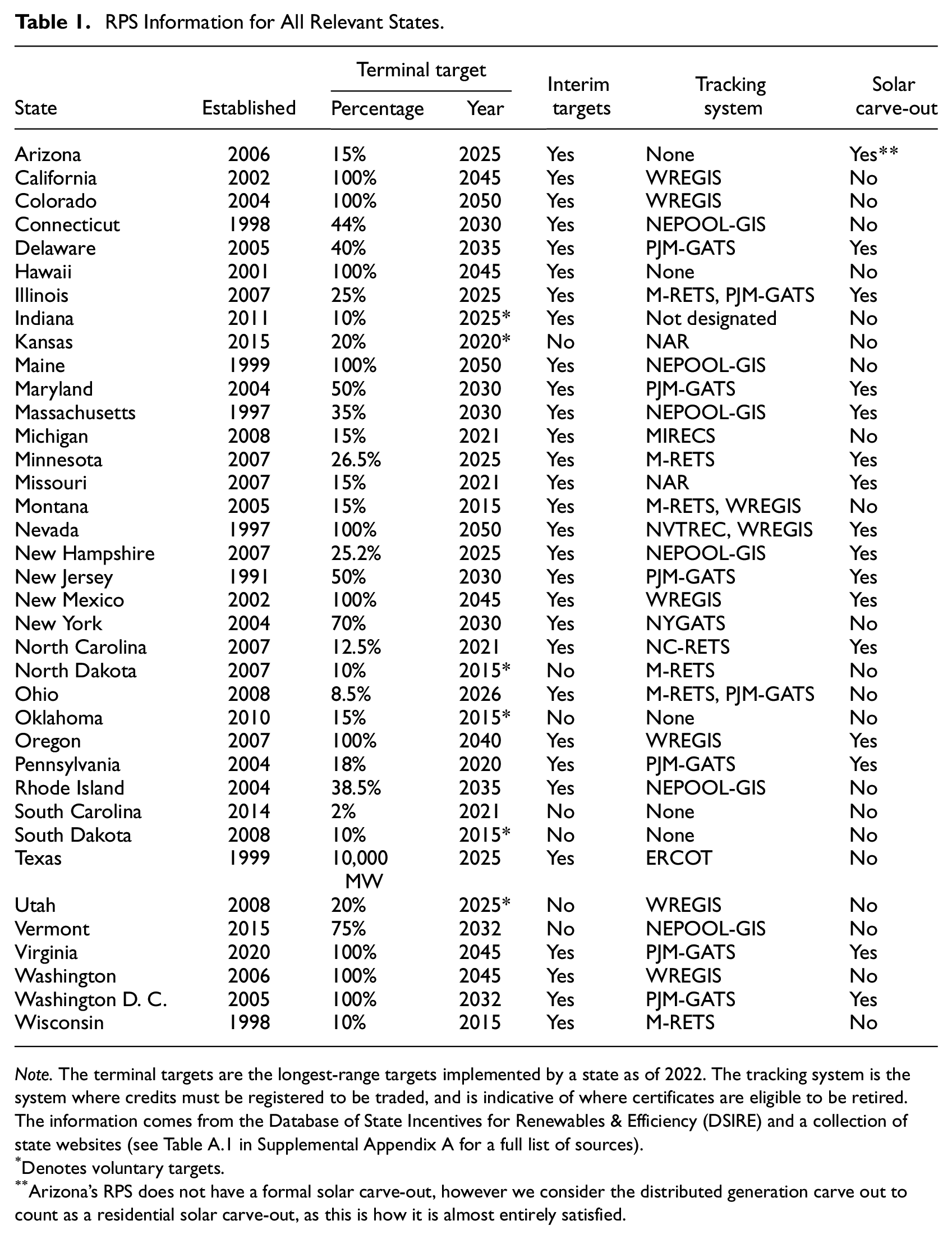
Note. The terminal targets are the longest-range targets implemented by a state as of 2022. The tracking system is the system where credits must be registered to be traded, and is indicative of where certificates are eligible to be retired. The information comes from the Database of State Incentives for Renewables & Efficiency (DSIRE) and a collection of state websites (see Table A.1 in Supplemental Appendix A for a full list of sources).

Denotes voluntary targets.

Arizona’s RPS does not have a formal solar carve-out, however we consider the distributed generation carve out to count as a residential solar carve-out, as this is how it is almost entirely satisfied.

Utilities may face two main constraints when fulfilling the RPS:

Interim annual targets: States often face interim goals that increase progressively toward a terminal target that is usually set five or ten years ahead. The RPS targets in New Jersey, for example, require 14 percent renewables by 2019, 16 percent by 2020, and 21 percent by 2021, eventually ramping up to 50 percent by 2030 (Database of State Incentives for Renewables and Efficiency 2021). While most states have set annual interim targets on a path toward meeting their final RPS goal, it is also quite common to specify such interim targets once every two, three, four, or five years. In addition, most states allow for banking of renewable energy credits.⁶ This allows utilities to flexibly comply with the interim targets by choosing their own multiple-year time path toward compliance.

Geographic trading restrictions: Utilities can only use RECs produced within their state or regional transmission organization to comply with the RPS. For example, RECs produced in the 13 states that are part of the PJM Interconnection,⁷ a regional transmission organization in the U.S. Northeast, can be used to comply with Pennsylvania’s RPS.

States’ RPS requirements can be met with multiple different sources of renewable energy and are sometimes called Tier/Class 1 requirements. In addition, states might also have a solar energy portfolio standard, also known as a solar carve-out. A solar carve-out requires a fraction of the RPS goal to be fulfilled exclusively with solar energy. In states with solar carve-outs utilities also purchase or generate solar RECs (SRECs). Figure 1 (top) presents a map of states that have an RPS or solar carve-out as of 2021. Additionally, in Figure 1 (bottom) we present a measure of states’ solar resource,⁸ and also highlight the borders of states with a solar carve-out. This map shows that the majority of states with a solar RPS are not in regions with high solar resource, hinting at a potential cost-inefficient allocation of solar installations. Table 2 presents the annual solar carve-out targets, as a percentage of total electricity sales, and geographic trading rules for the states with a solar carve-out in the period of 2015 to 2019.

Figure 1.

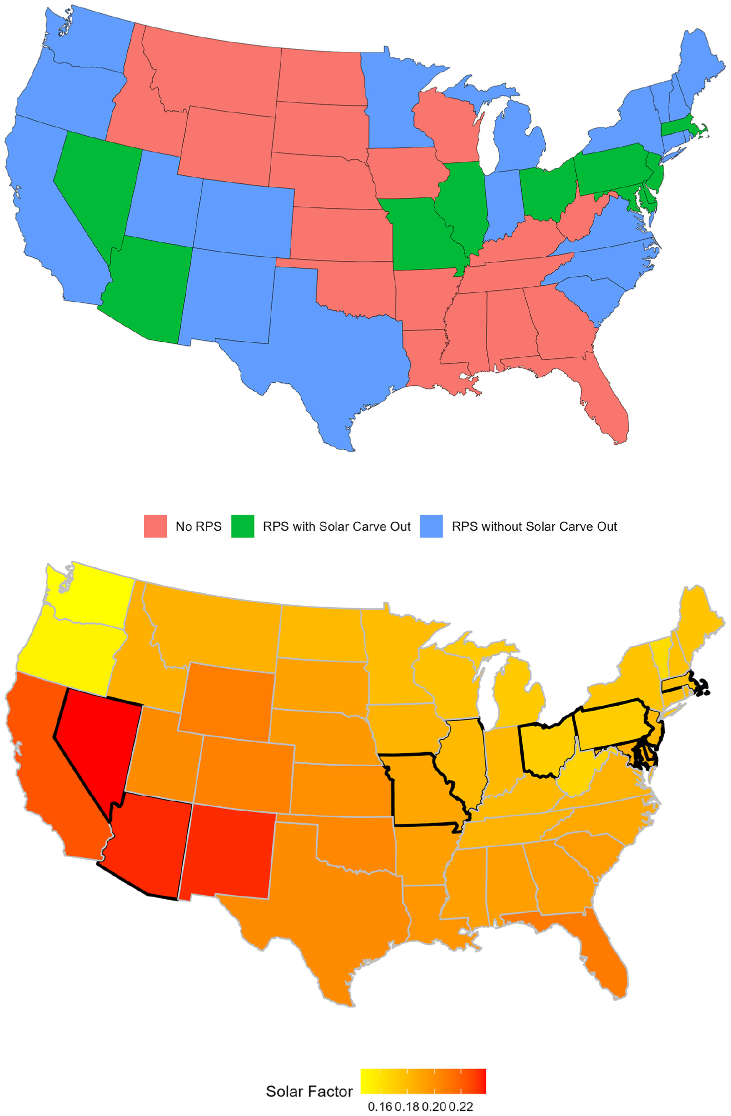
States with RPSs and solar carve-outs as of 2021.

Table 2.

Annual Solar RPS by State as Percentage of Statewide Electricity Sales, 2015 to 2019.

Year	AZ	DE	MD	MA	MO	NV	NH	NJ	NM	OR	PA
2015	1.50	1.00	0.50	2.60	0.10	1.00	0.30	2.75	3.00	0.04	0.25
2016	1.80	1.25	0.70	2.73	0.10	1.20	0.30	3.00	3.00	0.04	0.29
2017	2.10	1.50	1.15	5.09	0.10	1.20	0.30	3.20	3.00	0.04	0.34
2018	2.40	1.75	1.50	6.42	0.20	1.20	0.50	4.30	3.00	0.04	0.39
2019	2.70	2.00	5.50	6.66	0.20	1.20	0.60	4.90	3.00	0.04	0.44

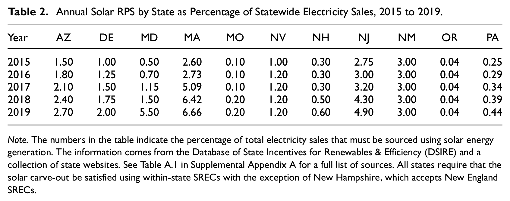
Note. The numbers in the table indicate the percentage of total electricity sales that must be sourced using solar energy generation. The information comes from the Database of State Incentives for Renewables & Efficiency (DSIRE) and a collection of state websites. See Table A.1 in Supplemental Appendix A for a full list of sources. All states require that the solar carve-out be satisfied using within-state SRECs with the exception of New Hampshire, which accepts New England SRECs.

Although RECs and SRECs both represent a megawatt hour of renewable energy, there are often different rules for how the two types of certificates can be used for compliance. For example, the majority of states with solar carve-outs require that the SRECs be produced within state. There are exceptions, such as New Hampshire, which allows SRECs from all of New England. Pennsylvania allowed SRECs from out of state until an amendment in 2017, which restricted the eligibility to only in-state SRECs. The motivation for this was largely the fact that as one of the only states that allowed its utilities to comply with SRECs purchased from other states, a majority of Pennsylvania’s solar credits were being generated in other states. Further, Pennsylvania was ranked nineteenth in the Solar Jobs Report of that year (The Solar Foundation 2017), which motivated local lawmakers to find ways to incentivize more solar installations in Pennsylvania.

The price of RECs and SRECs is determined by supply and demand, and reflects the shadow cost of complying with the RPS. REC revenues increase the profitability of new renewable energy projects enough to ensure that there are sufficient certificates in the market to satisfy the utilities’ demand. REC prices will increase until the revenue of the marginal project necessary to comply with the state’s RPS equals the project’s costs. State conditions like a steep marginal cost of renewable energy, or a highly ambitious RPS target, can lead to a high shadow cost of compliance, which is reflected in high REC prices. Therefore, differences in the price of renewable energy certificates across states and time indicate differences in the cost of compliance.

Figure 2 presents the SREC prices for eight states with a solar carve-out for the period of 2010 to 2019. The graph illustrates how the cost of complying with the states’ solar RPS varies significantly across time and states. In several states, the SREC price is an order of magnitude above wholesale power prices (typically in the $30–50 per MWh range), while SREC prices in other states are close to zero. This motivates the research question of this paper—the large dispersion in SREC prices across states and over time suggests that economic gains could be realized from equating the marginal cost of compliance in space and time.⁹

Figure 2.

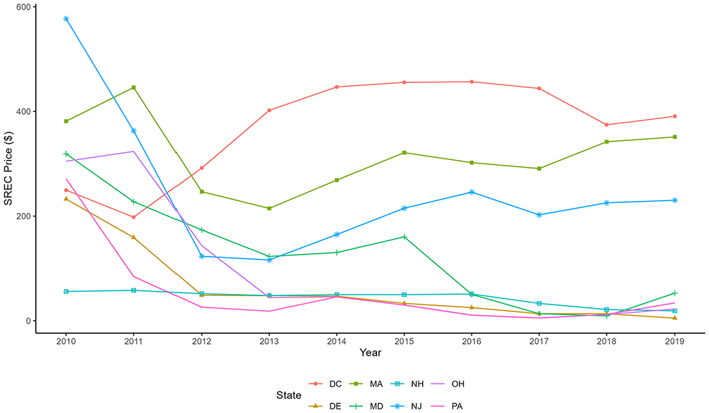
SREC prices in the U.S. Northeast, 2010 to 2019.

Although RPSs are the focus of this paper, they are not the only incentive program for renewable energy. Another important policy is the federal solar Investment Tax Credit (ITC). This program was implemented in 2006, and provided up to a 30 percent tax credit for solar systems over the sample period, on both residential and commercial properties (Pless and van Benthem 2019). Some states have also implemented state specific rebates. For example, in Maryland, the Residential Clean Energy Rebate Program offers monetary incentives to encourage the installation of residential solar water heating, solar photovoltaics, and geothermal heat pumps. Solar PV installations can receive a transfer of up to $1,000 per installation. Finally, most states have net metering policies. Households that generate electricity, for instance through solar panels on their roofs, can sell the excess electricity that they do not consume back to the grid. In the following sections, when we calculate the benefits of installing a solar panel, we incorporate not only SREC sales, but all benefits that a household would receive from their solar panels, including those mentioned above.

3. Empirical Strategy

In this section we present our strategy for obtaining state-level solar supply curves through a combination of estimation and calibration. We first present the problem a “national” planner faces when deciding how to satisfy an RPS.

3.1. National Planner’s Problem

Consider the problem of a national planner deciding how to allocate installations across states ( $s \in {1, \dots, S}$ ) and time ( $t \in {1, \dots, T}$ ) to minimize cost while achieving an RPS target in kW ( ${RPS}_{T}^{s}$ )¹⁰ subject to the states’ interim annual targets and geographic trading rules. A target is a defined level of cumulative installations that the planner must reach. Letting $q_{t}^{s}$ be the quantity of solar capacity allocated to state $s$ at time $t$ , this gives rise to the following cost minimization problem:

\begin{matrix} \min_{q_{t}^{s}} \sum_{s = 1}^{S} \sum_{t = 1}^{T} β^{t - 1} C_{t}^{s} q_{t}^{s} \\ s . t . q_{t}^{s} \geq 0, for t \in {1, \dots, T} \\ \sum_{j = 1}^{t} q_{j}^{s} \geq {RPS}_{t}^{s} for t \in {1, \dots, T}, for s \in {1, \dots, S} \\ (geographic trading rules) \\ \sum_{j = 1}^{t} \sum_{s = 1}^{S} q_{j}^{s} \geq \sum_{s = 1}^{S} {RPS}_{t}^{s} for t \in {1, \dots, T}, for s \in {1, \dots, S} \\ (interim annual targets) \end{matrix}

(1)

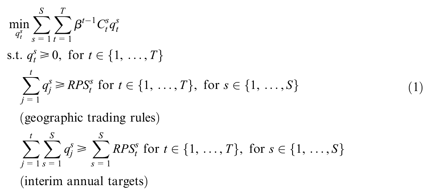
The planner might face four different scenarios:

1. All restrictions: The planner faces both state interim annual RPS targets and geographic trading restrictions. This is closest to the actual policy environment in most U.S. states.

2. Interim targets: There are state-level interim annual RPS targets, but cross-state trading is allowed.

3. Trading restrictions: There are no interim annual RPS targets, but cross-state trading is prohibited. The interim constraints in the planner’s problem collapse to a set of state-level RPS constraints that need to be satisfied by $T$ .

4. No restrictions: There are no state interim annual RPS targets and geographic trading restrictions in the planner’s cost minimization problem. These constraints collapse to a nationwide RPS constraint that needs to be satisfied by $T$ .

In our counterfactuals, we consider the period of 2015 to 2019 and include seven states with a solar carve-out in this period: Arizona, Delaware, Massachusetts, Missouri, New Hampshire, New Jersey, and New Mexico.¹¹ We convert the states’ RPS targets, generally set as a fraction of electricity sales (in kWh), into solar capacity (in kW) needed to comply with the RPS. Table 3 presents the interim targets (in MW) for each state. Note that these are cumulative RPS targets relative to 2014 installed capacity. Annual increases in the RPS correspond to the annual differences in targets for each state.

Table 3.

Solar RPS Targets by State in MW Relative to 2014 Installed Capacity, 2015 to 2019.

State	2015	2016	2017	2018	2019
AZ	16.17	48.47	68.96	106.73	149.17
DE	4.45	20.07	32.68	44.75	54.07
MA	92.40	150.15	346.86	457.96	457.96
MO	0.00	0.00	0.00	16.32	17.11
NH	0.56	0.95	0.95	9.18	12.28
NJ	40.55	134.60	205.47	397.69	498.50
NM	16.51	19.50	19.50	22.21	30.79
Total	170.64	373.74	674.42	1,054.84	1,219.88

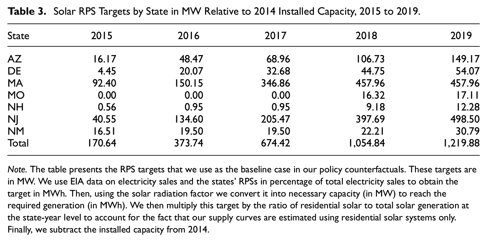
Note. The table presents the RPS targets that we use as the baseline case in our policy counterfactuals. These targets are in MW. We use EIA data on electricity sales and the states’ RPSs in percentage of total electricity sales to obtain the target in MWh. Then, using the solar radiation factor we convert it into necessary capacity (in MW) to reach the required generation (in MWh). We then multiply this target by the ratio of residential solar to total solar generation at the state-year level to account for the fact that our supply curves are estimated using residential solar systems only. Finally, we subtract the installed capacity from 2014.

3.2. Data Sources

We collect data from multiple sources. First, we use data on residential solar installations and prices from the Lawrence Berkeley National Laboratory (2020). For each installation we have information on the size of the system (capacity in kW), total installation cost (including cost of the panels), location (zip code), date of installation, rebates, an indicator for third party-owned systems (e.g., systems with a lease contract or a power purchase agreement), and other technical characteristics (module type, module manufacturer, module model, and number of inverters). The data cover the period from 2007 to 2019, although the coverage of this data set varies substantially across states.

We obtain information on states’ solar RPSs from a collection of state websites and from the Database of State Incentives for Renewables & Efficiency (DSIRE). This consists of states’ interim annual targets and RPS trading rules for the period of 2010 to 2019. In Section 4 we explain how we adjust the RPS targets to account for the fact that we only use data on residential installations to compute our supply curves. From the Energy Information Administration (EIA), we collect state-level data on solar energy generation (by sector and source) and total electricity generation for the period of 2015 to 2019.¹² We collect data on SREC prices for eight states from Barbose et al. (2019) for the period of 2010 to 2019. We combine these data sets to compute annual state solar targets in megawatts. See Supplemental Appendix C for details on data processing.

We compute a measure of solar radiation at the market level, which we call the solar radiation factor (SRF). We compute the SRF in three steps. First, we predict the expected generation (in kWh) of a system of 6.5 kW (the average in the data), located at the geographic center of the market. We obtain the expected generation from NREL’s PVWatts V6 API.¹³ Second, we compute the potential generation, defined as the generation a system would have if it produced at maximum capacity in every hour of the year (i.e., perfectly sunny days and only daylight hours). Finally, we compute the SRF as the ratio of expected to potential generation. This measure captures differences across markets in how much of a solar system’s potential is actually realized.

We compute electricity savings using average electricity rates data at the state level from the U.S. Energy Information Administration (2021) and collect data on state-level incentives from the Lawrence Berkeley National Laboratory (2020). Finally, we use population data from the U.S. Census Bureau (2021).

3.3. Calibration of Cost Curves

The necessary objects to solve the planner’s problem detailed in Section 3.1 are a discount rate for the social planner, state-year RPS targets (detailed in Table 3) and state-year installation cost functions $C_{t}^{s}$ . In this subsection, we briefly describe how to derive these cost curves from the data—a more detailed exposition can be found in Supplemental Appendix D.

We have in mind supply curves that are upward sloping within a given year and shift down over time as solar technology improves.¹⁴ Figure 3 illustrates this for two states in a given calendar year that have implemented the same RPS. The cost of increasing solar capacity in state A rises faster than in state B. To ensure compliance with the RPS, solar revenues (which are given by electricity savings, federal and state incentives, and SREC revenues) should be at least equal to the marginal cost of adding solar capacity at the RPS quantity. If electricity prices and incentives are equal across states, then SREC prices in state A must be higher than in state B to compensate for the difference in the marginal cost of solar installations.

Figure 3.

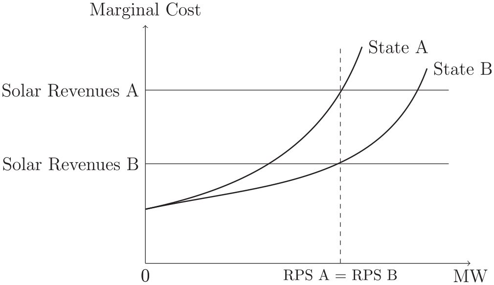
Solar supply curves example for two states with identical RPSs.

Our strategy for constructing these supply curves consists of a two-step method involving an estimation and a calibration component, using the data detailed in Section 3.2.¹⁵ In the first step, we note that supply and demand for solar energy varies within states (Gillingham et al. 2016). Therefore, we split states into distinct geographical markets and estimate market-level supply curves that we then aggregate to construct state-level supply curves. This approach exploits the disaggregate nature of our installation-level data.

Using the LBNL data on residential solar installations, we compute the quantity-per-capita installed (in kW per 1,000 people) and the average price per kW at the market-year level. Since this data gives us equilibrium prices and quantities of solar installation, we require a demand-shifting instrument to estimate supply curves. We use the SRF as an instrument, where exclusion is satisfied if the geographic efficiency of rooftop solar panels only affects demand and is uncorrelated with any other shifter of the marginal cost of solar installations. We use two-stage least squares (2SLS) to estimate supply curves with year-specific intercepts (to capture cost savings from technological improvements) and slopes that get flatter with total market size in kW (to capture differences in capacity for expansion across space):

(Price per kW)_{m, y} = θ (kW per 1000 people)_{m, y} + α_{y} + ϵ_{m, y}

(2)

where $m$ denotes market and $y$ calendar year.

A caveat of this instrumental-variables approach is that the presence of a competitive-effects channel could violate the exclusion restriction. If the market was imperfectly competitive, then markets with a higher SRF, and thus higher demand for solar, may attract more solar installation companies and thus increased competition that would result in lower costs (markups). This would introduce downward bias in our market-level slope estimates in equation (2), in turn understating the cost savings of a flexible policy design. We address this issue in more detail in Supplemental Appendix D.1 and through sensitivity analysis in Supplemental Appendix E.

We aggregate to the state level by summing across markets, with an additional calibration parameter $F$ —the capacity expansion factor—that determines the maximum level of solar capacity expansion within a market in a given year. The introduction of this parameter is motivated by the fact that, for a sufficiently high level of installations, markets would face a capacity constraint—for example, due to a limited supply of specialized workers or physical capital. This parameter imposes these constraints at the market level and rules out an unrealistic scenario in which, for any RPS size, the planner allocates the RPS target to a single market with the lowest marginal cost. Importantly, this parameter introduces convexity to our state-level supply curves, as a result of the market-level capacity constraints. That is, as the lower-cost markets reach their constraints, installations keep shifting to higher-cost markets with remaining capacity until the RPS is met.

Although this capacity expansion factor cannot be estimated directly from the data, we set it similar in size to equivalent parameters used in or derived from other models of the electricity sector (see Supplemental Appendix F). In our main specification we assume $F = 1.5$ , which essentially assumes that ramping up installations by more than 50 percent of the maximum amount installed over the period 2015 to 2019 would lead to steep cost increases. We are interested in the comparative statics when we vary this convexity; we perform a variety of robustness checks in Supplemental Appendices E and F which demonstrate that our qualitative conclusions hold under a broad set of parameter values. This step determines the slope of our state-level supply curves at all levels of possible solar expansion.

In the second step, we calibrate the intercepts of the state-level supply curves in each year by setting equal the marginal private benefit of expansion and the marginal cost of expansion (i.e., the supply curve) at the quantity we observe in the data. The marginal private benefit of expansion is given by the sum of electricity savings, SREC revenue, and other federal and state incentives, discounted and summed across time:

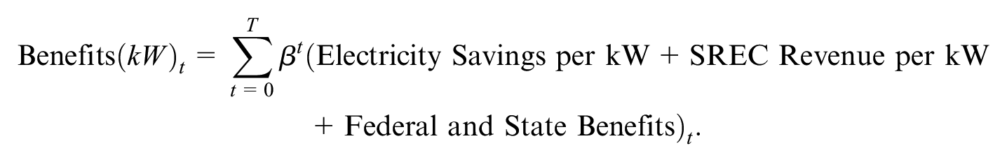
\begin{matrix} Benefits (kW)_{t} = \sum_{t = 0}^{T} β^{t} (Electricity Savings per kW + SREC Revenue per kW \\ + Federal and State Benefits)_{t} . \end{matrix}

where $T$ is the lifetime of a solar panel and $β$ is a discount factor.¹⁶

We vertically shift state-level supply curves until the marginal cost of solar expansion is equal to this marginal private benefit at the RPS-complying quantity. In order to simulate outcomes outside the capacity limits imposed by the market-level supply curves, we parameterize these supply curves using a double-exponential functional form, and test various other extrapolations for robustness. The second step is described in greater detail in Supplemental Appendix D.2.

Figure 4 presents the fitted supply curves of a subset of states with solar carve-outs for the years 2015 and 2019: Arizona, Massachusetts, New Jersey, and New Mexico (we use a subset for visual clarity). These curves illustrate the differences in cost both across states and years. Capacity expansion and technological improvements drive down the cost of new installations over time. Across states there is also interesting variation in the cost of solar energy. While it is relatively cheap to install a small amount of solar energy in New Mexico, its limited solar market increases the marginal cost rapidly. Meanwhile, Arizona possesses a much larger capacity than the other states and is able to install more solar before hitting the steeper part of its supply curve.

Figure 4.

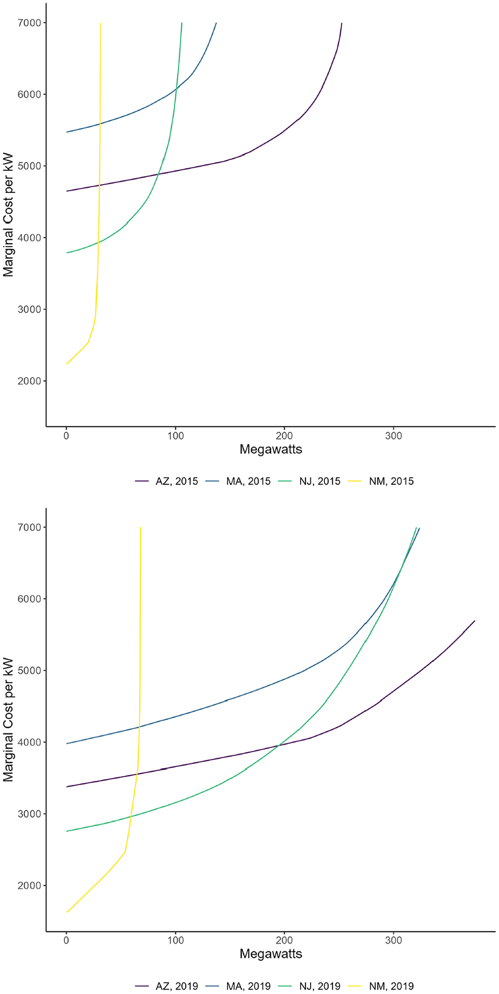
States’ solar supply curves: 2015 (top) and 2019 (bottom).

We caveat our results by emphasizing that our supply curve calibrations require some strong assumptions and several of our simulated policies are far out-of-sample. We therefore provide extensive robustness analysis in Supplemental Appendix E and conclude that, while the cost of meeting policy targets increases (decreases) with more (less) convex supply, the qualitative insights on relative inefficiencies of policy restrictions continue to hold. In addition, in Section 4 we present results where the RPS is satisfied on the steep part of the supply curve as well as on the flat part—covering a wide range of possible outcomes.

4. Counterfactual Simulations

In this section, we use our calibrated supply curves to simulate different policy environments using the social planner’s problem defined in Section 3.1. The planner must achieve a national RPS target given the states’ solar cost curves and subject to interim annual targets and trading restrictions. Using state-year supply curves derived as described in Section 3.3, we solve the planner’s problem for different sets of restrictions and RPS targets. We provide additional robustness checks in Supplemental Appendices E and F which vary functional form assumptions used in the construction of the supply curves.

4.1. Cost-minimizing Allocations for the Observed RPS

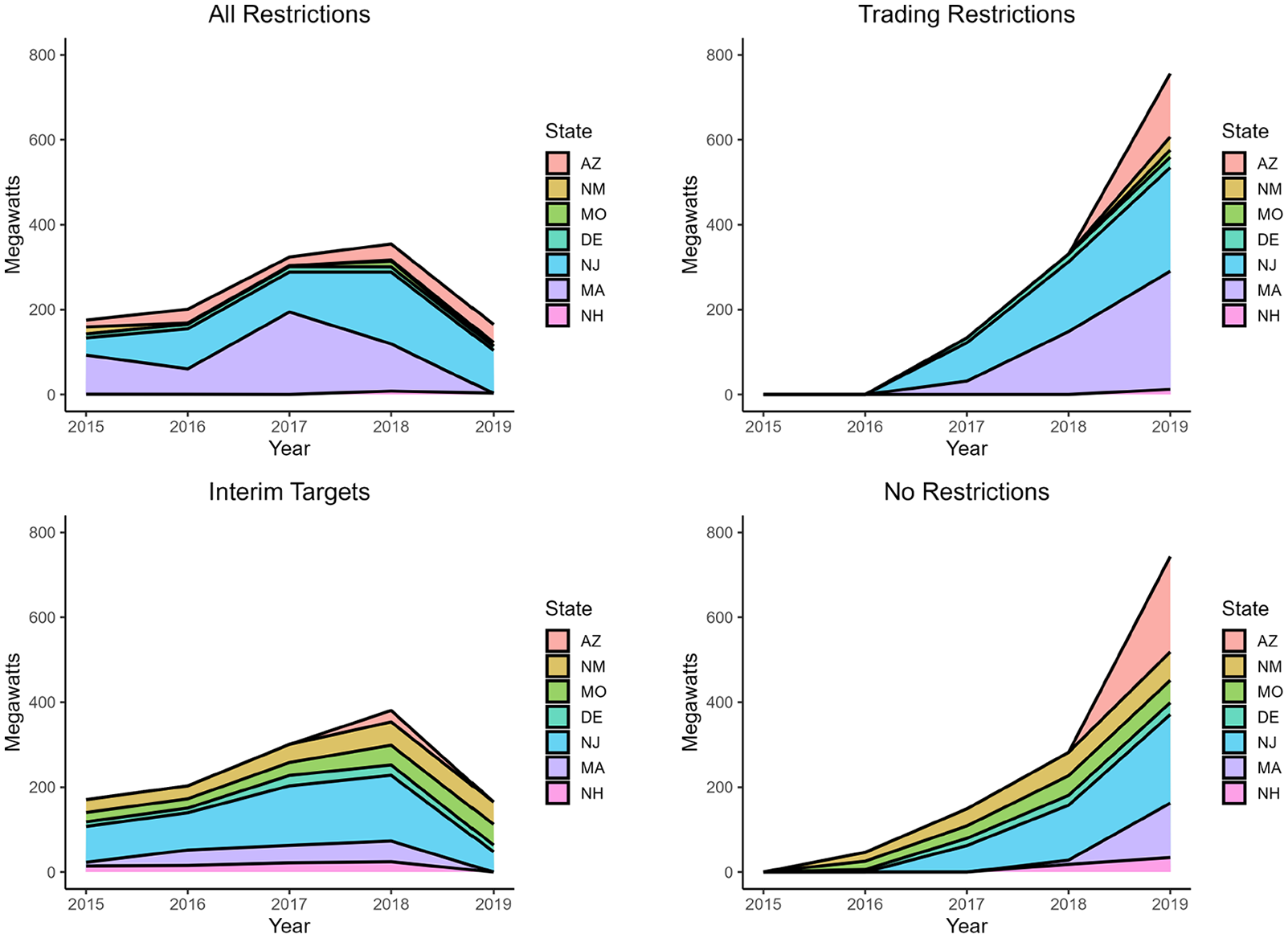
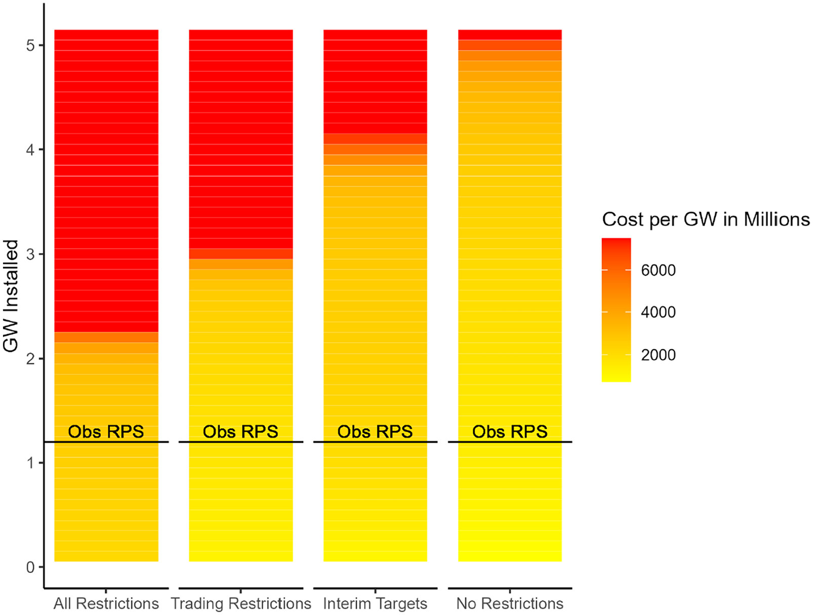
In our first counterfactual exercise we consider how the cost-minimizing allocations at our baseline RPS change under the four different scenarios. Figure 5 presents the allocation of new installations across states and years under each set of rules. For each year, the y-axis indicates total new capacity across all states. The color indicates what amount of that annual new capacity is installed in each state. Total added capacity across all states and years is equal to the combined RPS target, 1,220 MW, and is constant across scenarios.

Figure 5.

Cost-minimizing allocations under the four different scenarios.

The top panels require states to meet their targets with within-state installations. The bottom panels eliminate this restriction. Similarly, in the panels on the left the interim targets specified in the last row of Table 3 must be met. In the panels on the right we remove this requirement. We explain each figure in more detail below.

The top-left panel presents the allocation of new installations in the case with both annual targets and geographic trading restrictions. This figure plots the added capacity necessary to reach all interim targets. For example, the amount installed by Arizona in 2016 is equal to the difference between the 2016 and 2015 RPS targets for Arizona specified in Table 3. The first thing to note is that because of trading restrictions and the ambitious targets in the Northeast during our period of study, most of the installations occur in this region and, specifically, in Massachusetts and New Jersey. Also, the states’ schedules ramp up installations particularly in 2017 and 2018. These two years represent close to 56 percent of the installations.

We then consider how the allocation of installations changes in the absence of annual targets, while maintaining trading restrictions, that is, while still requiring states to reach their final 2019 target, but not necessarily the interim targets (top-right). Note that this is akin to allowing for SREC borrowing. It is clear that the initial schedule was not cost minimizing, and that a social planner would choose to back-load installations absent annual targets. Without annual targets, 84 percent of installations occur in the last two years. There are two main reasons for this. First, exogenous cost reductions over time favor later installations. Second, the continual expansion of capacity in all markets allows more installations in markets with flatter supply curves in later years.

Next, we compute the cost-minimizing allocations in the absence of trading restrictions but maintaining the states’ annual targets (bottom-left). This case is equivalent to a combined RPS with interim targets equal to the last row of Table 3. To minimize cost, the planner moves some installations from the Northeast (−20%) to the Southwest (+110%) relative to the status quo across all years.

When both trading restrictions and interim targets are lifted (bottom-right), the planner will simultaneously back-load and move some allocations in the Northeast (−35%) to the Southwest (+180%). Note that Arizona picks up more of the installations toward the end of the period.

To summarize, achieving cost-effectiveness involves a significant reallocation of installations across states, which is enabled by allowing for cross-state trading in SRECs. Removing interim annual targets would further enhance efficiency by taking advantage of changes in the cost of solar due to technological innovations.

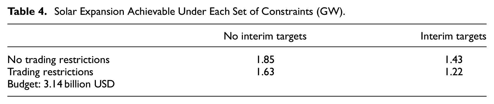
Finally, the previous set of counterfactual analyses asks what the cost-minimizing allocation of solar resource expansion is for a given RPS policy, where the primary object of interest for the policymaker is the total cost of compliance. We may instead ask what the quantity-maximizing allocation of solar resource expansion is for a given level of expenditure. This is the dual of the social planner’s problem described in Section 3.1. The solution to this dual problem shows what level of solar capacity expansion could have been achieved in the United States at no additional financial cost had the national policy been designed optimally.

Table 4 shows the results of this exercise. Under current RPS policies with interim targets and trading restrictions, the policy-mandated 1.22GW of total solar installation costs $3.14 billion on aggregate. At that same cost, an RPS with both restrictions lifted could have incentivized up to 1.85 GW of solar capacity expansion—a 52 percent larger increase. Compared to an RPS with both restrictions, an RPS with no interim targets but with trading restrictions would have yielded 34 percent greater expansion, and an RPS with no trading restrictions but with interim targets would have yielded 17 percent greater expansion.

Table 4.

Solar Expansion Achievable Under Each Set of Constraints (GW).

	No interim targets	Interim targets
No trading restrictions	1.85	1.43
Trading restrictions	1.63	1.22
Budget: 3.14 billion USD

4.2. Cost per Gigawatt for Different RPS Targets

We now explore how cost inefficiencies due to annual targets and trading rules vary for different RPS targets. Figure 6 presents the average cost per GW for the four planner’s scenarios as a function of the magnitude of the combined RPS targets across states.

Figure 6.

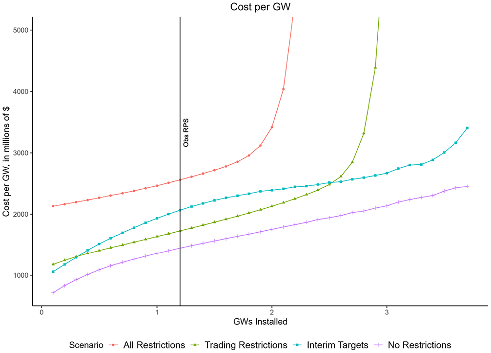
The cost of implementing renewable portfolio standards under various policy designs and overall stringency of the RPS target.

At the observed RPS (black vertical line), the cost is 33 percent lower without interim annual targets (green line) relative to the case with all restrictions (red line). Similarly, only eliminating geographic trading restrictions reduces the cost of implementing the observed RPS by 19 percent (blue line). Allowing for trade and removing annual targets leads to a cost reduction of 44 percent (purple line).

The cost differences across scenarios increase as the RPS becomes more ambitious. We consider the same percentage distribution of RPS targets across years and states as before, but we vary the overall RPS target.¹⁷ We find that, when the overall RPS doubles, implementing this more ambitious standard without restrictions is 90 percent cheaper than doing so with all restrictions. Eliminating either interim targets or geographic trading rules also leads to significant cost reductions—88 percent and 87 percent respectively. These cost differences increase for higher RPS targets as the flexibility benefits of trading and eliminating interim targets are especially valuable when the solar market is close to capacity.

In general, relaxing restrictions makes it possible to achieve larger RPS targets without reaching prohibitively high costs per GW. Figure 7 further illustrates this point. In the absence of any restrictions (fourth bar), the RPS target can be more than three times as high as the observed target (black horizontal line) while maintaining a cost per GW on the same level as that of the observed target with all restrictions (first bar, black line). Raising the RPS target by a factor of three would imply much higher costs if one imposed geographic trading rules (second bar), interim targets (third bar), or both (first bar).

Figure 7.

Cost per GW in each scenario for different RPS targets.

The results so far are based on supply curves with a maximum market-level capacity expansion factor of $F = 1.5$ (see Supplemental Appendix F for motivation). In Supplemental Appendices E.3 to E.6, we present the various results in this section using $F = 2$ and $F = 1.25$ , and altering the functional form of state-level supply curves. The larger capacity expansion factor shifts the state-level supply curves to the right, and reduces the costs of meeting increasingly ambitious RPS targets, but the qualitative results do not change and reveal similar types of inefficiencies of adding policy restrictions. In the case of steeper supply with $F = 1.25$ , the cost inefficiencies of the various policy restrictions—and therefore the benefits from more flexible program design—increase even faster as the RPS target is ramped up.

Together, these results show that interim annual targets and geographic trading restrictions can lead to significant cost inefficiencies in the implementation of RPSs. These inefficiencies become especially pronounced as we attempt to achieve higher levels of renewable energy generation.

4.3. Alternative RPS Schedules

The counterfactual exercises presented above used the annual state targets observed in the data as our baseline. In this section we explore the cost inefficiencies of alternative annual targets.

Specifically, we propose two simple schedules that policy makers might consider. First, a linearly increasing schedule where the same amount is installed every year until the target is reached. Second, an accelerating schedule where the amount installed increases every year until the target is reached. As a reference we also consider the observed schedule. Table 5 presents these three alternatives.

Table 5.

Percentage of final target reached each year.

	2015 (%)	2016 (%)	2017 (%)	2018 (%)	2019 (%)
Observed RPS	14	30.6	55.3	86.5	100
Linearly increasing RPS	20	40	60	80	100
Accelerating RPS	10	25	45	70	100

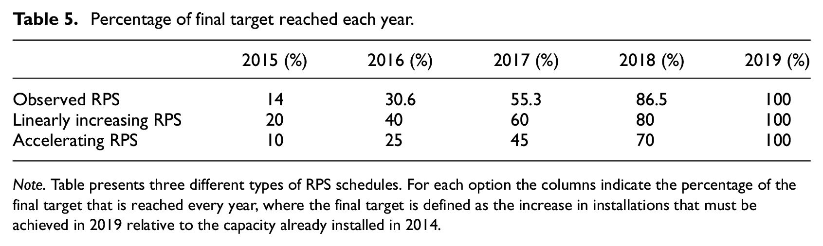
Note. Table presents three different types of RPS schedules. For each option the columns indicate the percentage of the final target that is reached every year, where the final target is defined as the increase in installations that must be achieved in 2019 relative to the capacity already installed in 2014.

We consider different combined RPS targets and for each we compute the cost of implementing the RPS in the absence of geographic trading restrictions. We then compute the cost increase that results from imposing interim annual targets for each RPS schedule and show the results in Figure 8.¹⁸

Figure 8.

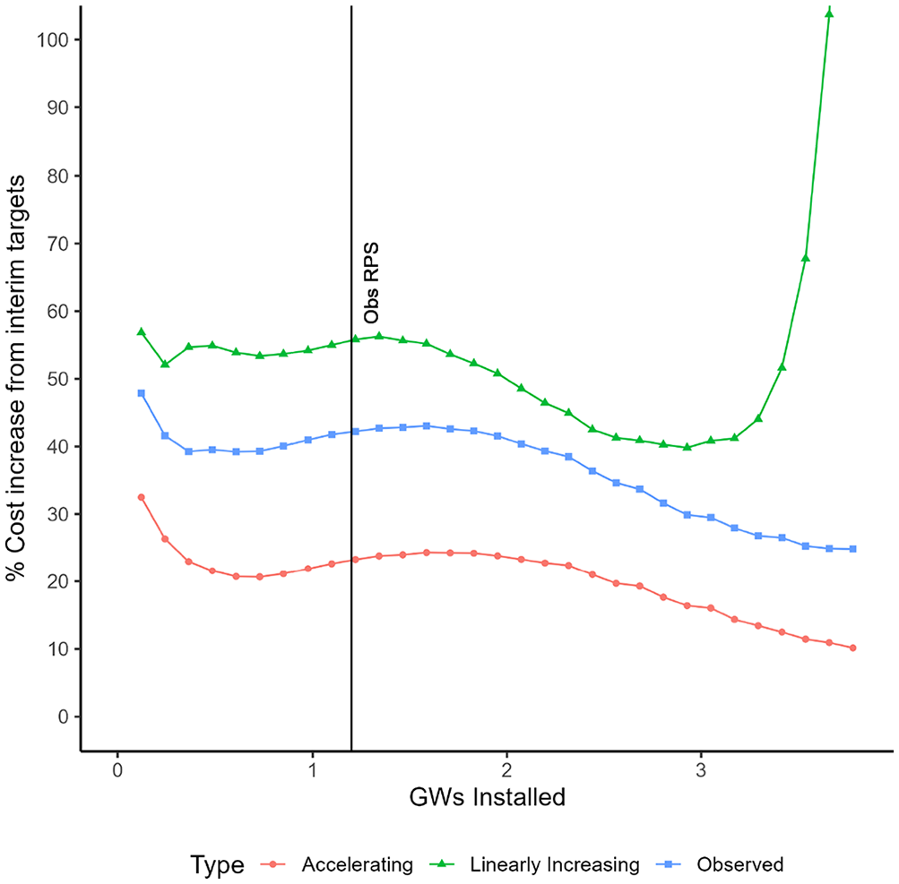
Cost increases of various interim annual target schedules.

The figure shows that for RPS targets of up to three times the observed one, any kind of interim targets will increase the cost, at times drastically. A clear pattern emerges that accelerating schedules are much less costly than linearly-increasing schedules, and the observed schedule is between the two. However, even the accelerating schedule we propose does not approximate the most cost-effective allocation across years, which would back-load installations even further.

These results show that these simple schedules can fail to significantly reduce the cost inefficiency associated with interim annual targets. To decrease the cost of implementing RPSs, policymakers must anticipate technological progress and other supply-side conditions to avoid cost-inefficient interim targets. In practice, this could be difficult and supports the use of more flexible RPS rules that allow for banking and borrowing of renewable energy credits, essentially removing or at least reducing the bindingness of interim targets, depending on the number of years over which SRECs can be borrowed.

4.4. Alternative RPS Allocations

In this section we consider a large number of potential allocations of RPS targets across states besides the one we observe in the data, and study how these affect the cost of implementation. To avoid staking a specific claim on the structure of these alternative allocations, we randomly allocate a given policy across states. We consider three different national targets: the one we observe in the data, half of this target, and a target that is 50 percent higher than the observed one. For each we compute 500 different random allocations. For each random allocation we compute the cost increase from restricting trade across states, in the absence of interim targets.¹⁹

Figure 9 presents a histogram of the cost increases for each combined RPS target. For an RPS of 50 percent of the observed one, most of the allocations across states result in moderate cost increases from imposing geographic trading restrictions (red bars). The median cost increase is 16 percent and the 90th percentile cost increase is 24 percent. For the observed RPS (green bars), the median cost increase remains moderate, at 12 percent. However, some allocations lead to larger cost inefficiencies. The 90th percentile in this case is 42 percent. For an RPS target of 1.5 times the observed RPS (blue bars), the cost of imposing geographic restrictions increases dramatically. In over 58 percent of the allocations the cost of implementing the RPS more than doubles. This happens because the RPS in one or more states reaches the very steep part of the solar supply curve. This suggests that highly-ambitious state targets can easily become prohibitively expensive when cross-state trading is restricted. Allowing for trade of renewable energy credits would mitigate these cost increases substantially.

Figure 9.

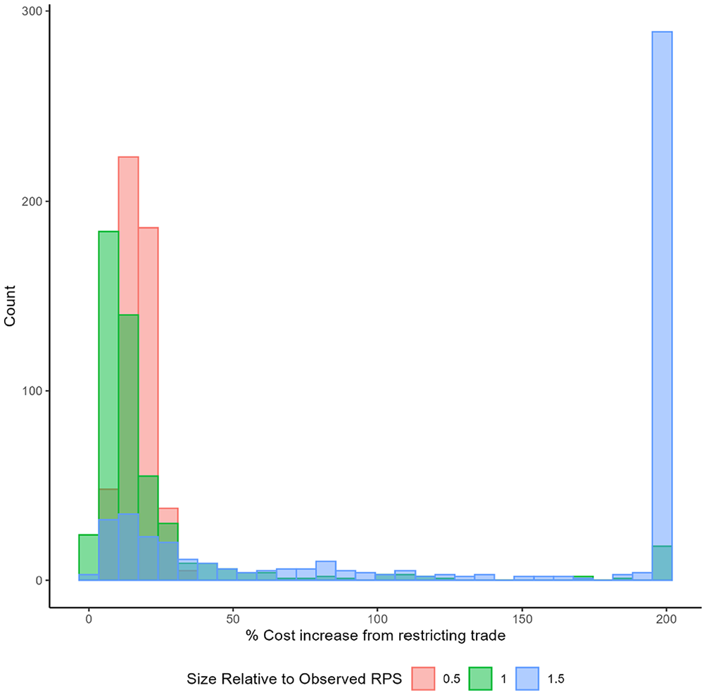
Cost increase of geographic trading restrictions for different cross-state RPS allocations and RPS targets.

5. Conclusion

In this paper we study the design of renewable energy portfolios standards. We focus on solar energy carve-outs and analyze two commonly observed market-design features of RPSs: cross-state trading restrictions and interim annual targets. Using historically observed RPSs and state-level solar supply curves that we construct using a combined estimation-calibration procedure, we find that these constraints can have a dramatic effect on the cost of reaching a given RPS target, especially when the standard is set ambitiously.

Allowing for cross-state trading could have reduced implementation costs by about a quarter and significantly changed the geographic distribution of new installations over the period 2015 to 2019. Similarly, removing interim annual RPS targets would have reduced costs by a third by back-loading installations. These cost reductions become much larger when we consider more ambitious RPS targets, that is, when solar supply becomes more capacity-constrained. Together our results suggest that trading, back-loading, banking, and borrowing can mitigate escalating costs and preserve the feasibility of RPSs.

These simulations directly speak to the discussion of the design of a federal renewable portfolio standard with a solar carveout. From a state perspective, local job creation and local environmental benefits might outweigh the cost reductions of allowing for cross-state trade, at least politically. From a federal perspective, however, a solar RPS with flexible trading rules would only reallocate local job creation and air pollution across the country, eliminating two of the strongest arguments in favor of geographic trading restrictions. A federal RPS that allows for cross-state trading would reduce total cost substantially relative to RPSs that are administered at the state level, with likely little overall impact on aggregate employment and pollution abatement benefits. Analogously, interim targets involve a trade-off. They may lower the risk of endline noncompliance, especially if agents are myopic or political turnover is high. Furthermore, forcing early action may help internalize learning-by-doing benefits and is desirable in light of the increasing marginal cost of delaying climate action. However, they can prevent solar producers from taking full advantage of cost reductions over time from technological progress. RPSs that forgo interim standards would almost certainly delay investment at the advantage of lower overall compliance cost.

Our results should be of interest to economists and practitioners of energy and environmental policy. Renewable portfolio standards are first-order policies to facilitate a shift toward a low-carbon economy. As policy ambitions ramp up, and the standards tighten, governments are well-advised to make sound and flexible policy-design choices that prevent unnecessary cost escalation—our results suggests that RPS policies that lack flexibility quickly become prohibitively expensive as the policy approaches annual capacity limits. With considerable uncertainty about the supply curve of solar within/across years, as policymakers increase RPSs, trading, banking, borrowing (at least over limited time periods), and convex interim targets can avoid escalating costs. These benefits need to be properly weighed against other objectives, such as moral hazard concerns with delaying investments in renewable energy, maintaining the policy’s political momentum and credibility, and potential political feasibility benefits of locally-directed policies (e.g., local job creation and air pollution improvements). However, the flexibility we describe has a proven track record: cross-state regional trading of Tier 1 RECs is commonly accepted; replicating the same model for SRECs would further enhance the cost-effectiveness of renewable energy standards.

Supplemental Material

sj-pdf-1-enj-10.1177_01956574251328253 – Supplemental material for Designing More Cost-effective Trading Markets for Renewable Energy

Supplemental material, sj-pdf-1-enj-10.1177_01956574251328253 for Designing More Cost-effective Trading Markets for Renewable Energy by Jose Miguel Abito, Felipe Flores-Golfin, Andrew J. Hinchberger, Arthur A. van Benthem and Gabrielle Vasey in The Energy Journal

Footnotes

Acknowledgements

We thank Kamen Velichkov and Yuyang Wang for excellent research assistance, numerous colleagues for useful comments and the Kleinman Center for Energy Policy, the Mack Institute, the Wharton Dean’s Research Fund, and Analytics at Wharton for generous support.

Declaration of Conflicting Interests

The author(s) declared no potential conflicts of interest with respect to the research, authorship, and/or publication of this article.

Funding

The author(s) received no financial support for the research, authorship, and/or publication of this article.

Supplemental Material

Supplemental material for this article is available online.

1

A state’s political inclination is predictive of the stringency of RPS targets and whether or not a state has an RPS at all (Fowler and Breen 2013; Huang et al. 2007; Lyon 2016; ).

2

Many academic and government reports have called for emissions to peak soon to avoid a “hard landing” with catastrophic climate-change impacts that would be ever-more expensive to avoid ().

3

Our supply curve is specified in terms of solar capacity in megawatts (MW) whereas RPSs are usually generation targets in megawatt hours (MWh). Later in the paper we convert generation targets into solar capacity needed to reach these targets.

4

Existing policies that overlap with RPSs include carbon-trading systems (Perino, Ritz and van Benthem 2022). The relevant one for the states we study is the Regional Greenhouse Gas Initiative (RGGI). During our sample period, however, prices were very low (in the $2–8 per ton range), suggesting that the RGGI emissions cap was hardly binding. Moreover, RGGI allowances were price-capped between $6 and 11 during this period (C2ES 2024). Hence, even in a counterfactual without the RPS, RGGI prices could not have risen to a level that would have triggered much solar investment: marginal abatement cost estimates for our sample period suggest solar breaking even at a carbon price of 60 euros per ton (McKinsey & Company 2009). RGGI was therefore highly unlikely to drive any growth in solar by itself.

5

Some exceptions, like Iowa and Texas, set their goals in terms of installed capacity (in MW).

6

It is common to have a certificate lifetime of three years (Delaware, New Hampshire, Missouri), however four years (New Mexico) and five years (New Jersey) also occur. In rare cases, such as Arizona, certificates (created after 1997) never expire, and can be retired at any point. We are not aware of any states that allow for long-term borrowing, that is, under-complying in the short run under the condition of making up for the shortfall in future years. By spacing out interim targets over multiple years, several states implicitly allow for short-run borrowing within such a compliance period. One example is California, which allows for short-run borrowing through interim annual RPS targets with three-year compliance periods ().

7

These states are Delaware, Illinois, Indiana, Kentucky, Maryland, Michigan, New Jersey, North Carolina, Ohio, Pennsylvania, Tennessee, Virginia, Washington DC, and West Virginia.

8

See Section D.1 for a detailed explanation of this measure.

9

In we present an equivalent graph with REC prices. REC prices are considerably lower than SREC prices. Given that solar credits can be used to comply with both the Tier/Class 1 requirements and the (more binding) solar carve-out, the price of SRECs must be at least as high as that of Tier/Class 1 RECs.

10

As explained in Section 2, RPSs are usually set as a percentage of generation (i.e., in kWh). However, to match the units of our cost curves (to be discussed in Section 3.3), we convert these RPS targets into capacity (in kW) needed to reach said targets. State-year installation cost functions are denoted C t s . explains this conversion.

11

We do not include the other five states with a solar carve-out due to limitations in the coverage of the LBNL and EIA data that do not allow us to construct a solar supply curve for Illinois, Maryland, Nevada, Ohio, and Pennsylvania.

12

For solar energy, solar residential, and electricity generation data, we use .

13

See for additional details.

14

Upward- sloping supply is a natural assumption in many markets; in the case of solar it could be driven by increasing costs of qualified labor, parts, permitting, and access to capital as installations expand.

15

We summarize the procedure here. For further details, see .

16

We set the discount factor equal to 0.8. This choice is based on evidence that consumers heavily discount the benefits of solar technologies ().

17

This distribution is obtained by dividing each element of by the total RPS target (1,220 MW).

18

In we compute the cost of implementing the RPS with geographic trading restrictions and with annual targets as described above. Our results in this case are similar to the ones presented in this section. The cost of imposing interim targets of any type is even higher when we also impose geographic trading restrictions and the cost ranking of the three alternatives does not change.

19

In we present the cost distribution with interim targets in place.

References

Barbose

Darghouth

Elmallah

Forrester

Millstein

Rand

Cotton

Sherwood

O’Shaughnessy

2019. “Tracking the Sun: Pricing and Design Trends for Distributed Photovoltaic Systems in the United States – 2019 Edition.” Technical Report, Lawrence Berkeley National Laboratory, Berkeley, CA.

Barbose

G. L.

2021. “U.S. Renewables Portfolio Standards 2021 Status Update: Early Release.” Technical Report. https://emp.lbl.gov/publications/us-renewables-portfolio-standards-3. Accessed September 3, 2023.

Bollinger

Gillingham

2019. “Learning-by-Doing in Solar Photovoltaic Installations.”SSRN2342406.

Burr

2016. “Subsidies and Investments in the Solar Power Market.” Working Paper, University of Colorado at Boulder, Boulder, CO.

C2ES. 2024. “Regional Greenhouse Gas Initiative (RGGI).”https://www.c2es.org/content/regional-greenhouse-gas-initiative-rggi/. Accessed June 11, 2024.

CA Public Utilities Commission. 2022. “Renewables Portfolio Standard (RPS) Program.”https://www.cpuc.ca.gov/rps/. Accessed September 2, 2023.

Cullen

2013. “Measuring the Environmental Benefits of Wind-Generated Electricity.”American Economic Journal: Economic Policy 5 (4): 107–33.

Database of State Incentives for Renewables and Efficiency. 2021. “Programs - Renewable Portfolio Standards.”https://programs.dsireusa.org/system/program. Accessed July 2, 2023.

De Groote

Verboven

, 2019. “Subsidies and Time Discounting in New Technology Adoption: Evidence from Solar Photovoltaic Systems.”American Economic Review 109 (6): 2137–72.

10.

del Río

. 2005. “A European-Wide Harmonised Tradable Green Certificate Scheme for Renewable Electricity: Is It Really So Beneficial?”Energy Policy 33 (10): 1239–50.

11.

Deschenes

Malloy

McDonald

2023. “Causal Effects of Renewable Portfolio Standards on Renewable Investments and Generation: The Role of Heterogeneity and Dynamics.”Resource and Energy Economics 75: 101393.

12.

Dorsey

. Forthcoming. “Solar Market Frictions: The Role of Platforms and Policies.” The Review of Economics and Statistics.

13.

Feldman

Levinson

2023. “Renewable Portfolio Standards.”The Energy Journal 44 (5): 1–20.

14.

Figueres

Schellnhuber

H. J.

Whiteman

Rockström

Hobley

Rahmstorf

2017. “Three Years to Safeguard our Climate.”Nature 546: 593–5.

15.

Fischer

2009. “Renewable Portfolio Standards: When Do They Lower Energy Prices?”Energy Journal 30 (4): 81–100.

16.

Fischer

Newell

R. G.

2008. “Environmental and Technology Policies for Climate Mitigation.”Journal of Environmental Economics and Management 55: 142–62.

17.

Fowler

Breen

2013. “The Impact of Political Factors on States’ Adoption of Renewable Portfolio Standards.”The Electricity Journal 26 (2): 79–94.

18.

Friedrich

Pickens

2020. “World’s Top 10 Emitters.”World Resources Institute. https://www.wri.org/insights/interactive-chart-shows-changes-worlds-top-10-emitters. Accessed September 3, 2023.

19.

Fullerton

2025. “What Determines Effectiveness of Renewable Energy Standards?: General Equilibrium Analytical Model and Empirical Analysis.”Journal of the Association of Environmental and Resource Economists 12 (1): 65–103.

20.

Gerarden

2021. “Demanding Innovation: The Impact of Consumer Subsidies on Solar Panel Production Costs.” Working Paper, Cornell University, Ithaca, NY.

21.

Gillingham

Deng

Wiser

Darghouth

Nemet

Barbose

Rai

Dong

2016. “Deconstructing Solar Photovoltaic Pricing.”The Energy Journal 37 (3): 231–50.

22.

Gowrisankaran

Reynolds

S. S.

Samano

2016. “Intermittency and the Value of Renewable Energy.”Journal of Political Economy 124 (4): 1187–234.

23.

Greenstone

Nath

2020. “Do Renewable Portfolio Standards Deliver Cost-Effective Carbon Abatement?” BFI Working Paper, Becker-Friedman Institute, Chicago, IL.

24.

Heeter

Barbose

Bird

Weaver

Flores-Espino

Kuskova-Burns

Wiser

2014. “Survey of State-Level Cost and Benefit Estimates of Renewable Portfolio Standards.” Technical Report, National Renewable Energy Lab, Golden, CO.

25.

Heeter

Speer

Glick

M. B.

2019. “International Best Practices for Renewable Portfolio Standard (RPS) Policies.” NREL/TP-6A20-72798, National Renewable Energy Laboratory, Golden, CO.

26.

Huang

M.-Y.

Alavalapati

J. R. R.

Carter

D. R.

Langholtz

M. H.

2007. “Is the Choice of Renewable Portfolio Standards Random?”Energy Policy 35 (11): 5571–5.

27.

Hughes

J. E.

Podolefsky

2015. “Getting Green with Solar Subsidies: Evidence from the California Solar Initiative.”Journal of the Association of Environmental and Resource Economists 2 (2): 235–75.

28.

Joskow

P. L.

2011. “Comparing the Costs of Intermittent and Dispatchable Electricity Generating Technologies.”American Economic Review 101 (3): 238–41.

29.

Lamp

2023. “Sunspots That Matter: The Effect of Weather on Solar Technology Adoption.”Environmental and Resource Economics 84: 1179–219.

30.

Lawrence Berkeley National Laboratory. 2020. “Distributed Solar Public Data.”https://emp.lbl.gov/tracking-the-sun. Accessed September 3, 2023.

31.

Liao

2020. “Weather and the Decision to Go Solar: Evidence on Costly Cancellations.”Journal of the Association of Environmental and Resource Economists 7 (1): 1–33.

32.

Lyon

T. P.

2016. “Drivers and Impacts of Renewable Portfolio Standards.”Annual Review of Resource Economics 8 (1): 141–55.

33.

Lyon

T. P.

Yin

2010. “Why do States Adopt Renewable Portfolio Standards? An Empirical Investigation.”The Energy Journal 31 (3): 133–57.

34.

McKinsey & Company. 2009. “Pathways to a Low-Carbon Economy.” Technical Report, February 2021. https://www.mckinsey.com/capabilities/sustainability/our-insights/a-cost-curve-for-greenhouse-gas-reduction.

35.

PA Department of Environmental Protection. 2018. “Pennsylvania’s Solar Future Plan.”https://www.dep.pa.gov/Business/Energy/OfficeofPollutionPrevention/SolarFuture/Pages/Pennsylvania\%27s-Solar-Future-Plan.aspx. Accessed September 3, 2023.

36.

Palmer

Burtraw

2004. Electricity, Renewables, and Climate Change: Searching for a Cost-effective Policy. Washington, DC: Resources for the Future.

37.

Palmer

Burtraw

2005. “Cost-effectiveness of Renewable Electricity Policies.”Energy Economics 27: 873–94.

38.

PennFuture. 2018. “What Act 40 Means for Solar Energy in PA.”https://www.pennfuture.org/Blog-Item-What-Act-40-Means-for-Solar-Energy-in-PA. Accessed September 3, 2023.

39.

Perino

Ritz

R. A.

van Benthem

A. A

. 2022. “Overlapping Climate Policies.” NBER Working Paper No. 25643, National Bureau of Economic Research, Cambridge, MA. https://www.nber.org/papers/w25643.

40.

Pless

van Benthem

A. A.

2019. “Pass-Through as a Test for Market Power: An Application to Solar Subsidies.”American Economic Journal: Applied Economics 11 (4): 367–401.

41.

Pritchard

Z. D.

Mills

2021. “Renewable Energy Requirements on the Ballot: An Analysis of County-Level Voting Results.”Energy Policy 148: 111949.

42.

Sexton

Kirkpatrick

A. J.

Harris

R. I.

Muller

N. Z.

2021. “Heterogeneous Solar Capacity Benefits, Appropriability, and the Costs of Suboptimal Siting.”Journal of the Association of Environmental and Resource Economists 8 (6): 1209–44.

43.

Söderholm

2008. “The Political Economy of International Green Certificate Markets.”Energy Policy 36 (6): 2051–62.

44.

The Solar Foundation. 2017. “National Solar Jobs Census 2017.”https://mdvseia.org/wp-content/uploads/2018/03/SolarJobsCensus2017.pdf. Accessed December 3, 2023.

45.

United Nations Environment Programme. 2023. “Emissions Gap Report 2023: Broken Record – Temperatures Hit New Highs, Yet World Fails to Cut Emissions (Again).”United Nations Environment Programme, Nairobi. doi:10.59117/20.500.11822/43922.

46.

Upton

G. B.

Jr. Snyder

B. F.

2017. “Funding Renewable Energy: An Analysis of Renewable Portfolio Standards.”Energy Economics 66: 205–216.

47.

U.S. Census Bureau. 2021. “Relationship Files.”https://www.census.gov/geographies/reference-files/2010/geo/relationship-files.html. Accessed August 12, 2023.

48.

U.S. Energy Information Administration. 2020. “Renewable Energy Explained: Portfolio Standards.” U.S. Energy Information Administration – EIA – Independent Statistics and Analysis. https://www.eia.gov/energyexplained/renewable-sources/portfolio-standards.php. Accessed September 3, 2023.

49.

U.S. Energy Information Administration. 2021. “Electricity Data.”https://www.eia.gov/electricity/data.php. Accessed September 2, 2023.

50.

van Benthem

A. A.

Gillingham

Sweeney

J. L.

2008. “Learning-by-Doing and the Optimal Solar Policy in California.”The Energy Journal 29 (1): 131–51.

Supplementary Material

Please find the following supplemental material available below.

For Open Access articles published under a Creative Commons License, all supplemental material carries the same license as the article it is associated with.

For non-Open Access articles published, all supplemental material carries a non-exclusive license, and permission requests for re-use of supplemental material or any part of supplemental material shall be sent directly to the copyright owner as specified in the copyright notice associated with the article.

0.00 MB

6.25 MB