What Can We Learn About Carbon-reducing Innovations From the Joint Dynamics of CO 2 Emissions and GDP?

Abstract

Technological innovations targeting energy efficiency, carbon storage, and clean energy are often promoted as solutions to reduce emissions without sacrificing economic growth. However, theoretical studies offer conflicting views on the feasibility of this approach, and empirical assessments at the aggregate level are sparse. This paper contributes new evidence on the macroeconomic implications of carbon-reducing technological innovations. We analyze the joint dynamics of U.S. per capita emissions and GDP and identify a novel shock that lowers emissions without reducing economic output. This statistical shock is uncorrelated with past macroeconomic variables, energy prices, estimates of the leading macroeconomic shocks, and measures of environmental policy stringency. Our novel shock exhibits characteristics of an energy demand-reducing shock specific to the U.S. energy market, with pronounced effects concentrated in the residential and commercial sectors. This shock appears to be linked to improvements in energy efficiency, possibly stemming from changes in energy requirements for homes and buildings. These improvements may result from energy policies, occur exogenously, or reflect shifts in preferences for energy conservation.

JEL Classification: E32, Q43, Q50, Q55

1. Introduction

Technological innovations aimed at energy efficiency, carbon storage, and clean energy have been promoted as possible solutions to reduce carbon dioxide (CO₂) emissions ¹ without sacrificing economic growth. However, theoretical studies in environmental economics offer conflicting views on the feasibility of avoiding the trade-off between environmental protection and economic growth or even reducing emissions through technological innovations. The paucity of rigorous empirical evaluations of theoretical predictions poses a significant challenge in distinguishing between alternative scenarios with diverse implications. Without a clear understanding of the plausibility of these scenarios, researchers, and policymakers may have the flexibility to choose options that align with their priorities and preferences, risking adverse economic outcomes.

We provide new evidence on the role of technological innovations in mitigating emissions. To this end, we perform a retrospective analysis of the U.S. data, focusing on different types of carbon-reducing technological (CRT) innovations. We examine energy-efficiency improvements, advancements in producing carbon-free energy and less-polluting fossil fuels, and carbon capture and storage. Various classes of general equilibrium models study the macroeconomic implications of these innovations, typically analyzing one CRT type at a time. ² A recurrent theoretical result across methodologies and various types of technology is the divergence of predictions about the impacts of CRT innovations on emissions and aggregate output. For the same CRT type, and often in the same model, some specifications demonstrate the feasibility of reducing emissions without impeding growth, whereas others assert that emissions mitigation comes at the cost of lower output or even predict a rise in emissions (Table 1). ³ In this paper, we aim to provide empirical insights into whether the potential of CRT innovations to achieve simultaneous reductions in emissions and sustained economic growth has been realized in practice.

Table 1.

Summary of Short-run Effects of CRT Innovations From General Equilibrium Models.

(a) Exogenous energy-efficiency improvements
Allan et al. (2009), Böhringer and Rivers (2021), Diaz and Puch (2019), Fullerton and Ta (2020), Lemoine (2020), Saunders (2008), Turner (2009)	EN & EM may ↓ or ↑ GDP may ↑ or ↓ P ↓ or unchanged
Huynh (2016)—Energy-efficiency shock to consumer durables	EN & EM ↓, GDP ↑, PE ↓ Household EN ↓
Huynh (2016)—Energy-efficiency shock to productive capital	EN & EM ↓, GDP ↑, PE ↓ Household EN ↑
(b) Endogenous energy-efficiency improvements
Alpanda and Peralta-Alva (2010), Hassler, Krusell and Olovsson (2021), Kehoe and Atkeson (1999), Lemoine (2020), Wei (2003)	EN & EM ↓ GDP may ↑ or ↓ PE ↑
(c) Advancements in producing low-carbon and carbon-free energy
Chang, Wang and Shieh (2018), Greaker and Popp (2022), Fischer and Heutel (2013), Popp, Newell and Jaffe (2010)	EM may ↓ or ↑, GDP may ↑ or ↓ Fossil PE ↑, Clean energy PE ↓
(d) Advancements in producing cleaner fuels
Arora (2014), Chang, Wang and Shieh (2018), Dissou and Karnizova (2016)	EM ↑ but may ↓, GDP ↑ Oil/gas PE ↓ or unchanged
(e) Advancements in carbon capture, utilization and storage
Grimaud and Rouge (2014), Kalkuhl, Edenhofer and Lessmann (2015), Lee, Lee and Koo (2022)	EM may ↓ or ↑, GDP may ↑ or ↓

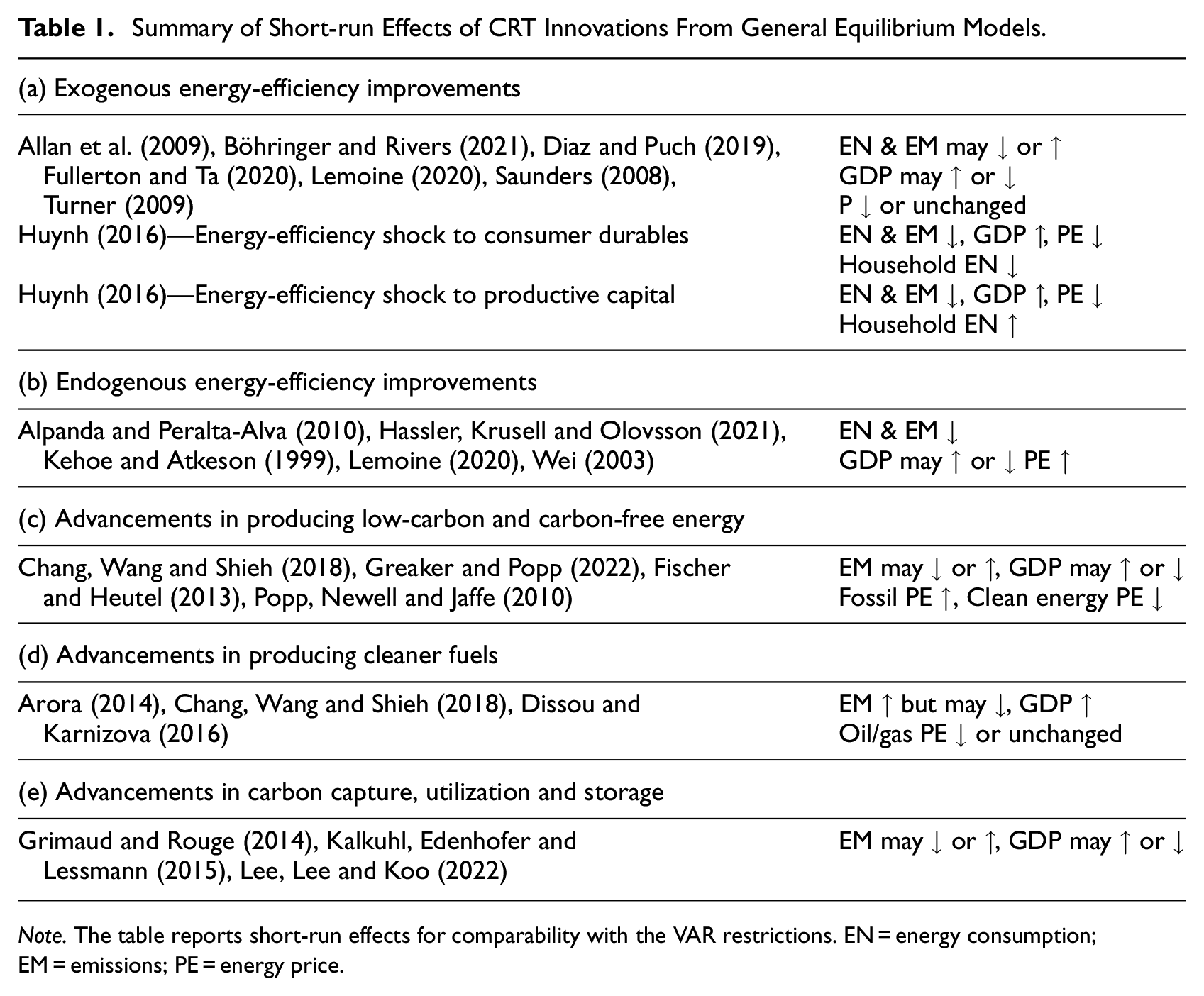
Note. The table reports short-run effects for comparability with the VAR restrictions. EN = energy consumption; EM = emissions; PE = energy price.

Theoretical debates on the impact of CRT innovations on emissions and aggregate output inspire us to focus on the joint behavior of these two variables. We start by noting that in many quarters U.S. emissions grow less than expected even as GDP (gross domestic product) grows faster than expected. We then propose to statistically decompose the joint error in forecasting emissions and economic growth into two distinct components. The first component, referred to as the positive correlation (PC) shock, has the property to slow GDP growth if emissions fall. The second component, the negative correlation (NC) shock, moves the two variables in opposite directions. Our primary interest lies in understanding the NC shock. ⁴

We hypothesize that the NC shock reflects CRT innovations. To evaluate our hypothesis, we analyze the NC shock’s impact across U.S. macroeconomic and environmental indicators. For each CRT innovation, we systematically identify key variables, such as energy prices, that are crucial for understanding its transmission in general equilibrium models. For this part of the analysis, we focus exclusively on theoretical specifications where CRT innovations reduce emissions. Our objective is to assess whether the empirical effects of the NC shock on U.S. variables align with the theoretical predictions associated with CRT innovations. The consistency between empirical results and theoretical predictions would suggest that the NC shock reflects a specific CRT type. ⁵

Formally, we estimate the NC and PC shocks via sign restrictions in a vector autoregressive model (VAR) with total emissions and GDP. Despite its small size, our VAR is informationally sufficient, as defined by Forni and Gambetti (2014), for the NC shock. Empirical orthogonality tests confirm that the NC shock is uncorrelated with past macroeconomic variables, energy prices, estimates of the leading macroeconomic shocks, and measures of environmental policy stringency. ⁶ In our VAR, a positive NC shock that decreases total per capita emissions by 1 percent, increases the posterior median of per capita GDP by 0.4 percent on impact. Emissions intensity persistently declines by 1 percent, driven by higher GDP and reduced fossil fuel consumption.

We use distributed lag models (DLMs) to estimate the impact of the NC shock on U.S. indicators. This approach imposes no constraints on the economic responses, allowing the estimates to be entirely data-driven. This feature is especially advantageous when the theoretical literature presents conflicting views on the macroeconomic impacts of CRT innovations. The DLM analysis provides valuable insights into the economic transmission of the NC shock.

At the aggregate level, a positive NC shock that increases GDP results in a reduction in both energy use and prices. The shock is positively related to several economy-wide proxies for energy efficiency. At the sectoral level, the NC shock affects energy users differently in terms of emissions, energy consumption, prices, and measured energy efficiency. The residential and commercial sectors react the most. Following a positive NC shock, energy consumption and prices in these sectors decrease, while measured energy efficiency and the consumption of non-energy goods and services rise. Collectively, these economic responses indicate that the NC shock displays the characteristics of an energy demand-reducing shock specific to the U.S. energy market, potentially originating in the residential and commercial sectors.

Further insights emerge from analyzing the impact of the NC shock on U.S. energy producers and key macroeconomic variables. A positive NC shock leads to a decline in natural gas extraction and petroleum refinery output, while leaving non-fossil energy production unaffected. The producer price of natural gas decreases, whereas oil prices—primarily determined by global markets—remain unaffected. Additionally, we document an expansion in consumption, investment, hours worked, labor productivity, and a boom in the stock market. These empirical responses are also suggestive of an energy-demand reducing shock specific to the U.S. energy market.

Exogenous energy-efficiency improvements, particularly those that reduce energy consumption in homes and buildings, may explain the observed aggregate and sector-specific responses triggered by a positive NC shock. However, alternative explanations exist. Changes in energy-efficiency standards could stimulate technological innovation aimed at reducing energy consumption, thereby serving as a causal driver of the NC shock. Additionally, shifts in preferences for energy conservation may be observationally equivalent to exogenous energy-efficiency shocks. Furthermore, these preference shifts may themselves stem from changes in energy conservation policies. Our empirical methodology is unable to differentiate between these potential drivers.

Reconciling our empirical findings with CRT innovations that influence the U.S. energy market through supply-side mechanisms presents a challenge. Such innovations would typically increase cleaner energy production, but this response is not observed following a positive NC shock. It is important to emphasize that our results do not imply a lack of innovations aimed at improving production efficiency or reducing costs, nor do they diminish the significance of such innovations in achieving emissions reductions. However, they suggest that these innovations were unlikely to be the primary drivers of the NC shock within our sample. They may have been costly at the aggregate level, reducing GDP, or their impact on the NC shock may have been small, overshadowed by shocks to energy demand.

Our work contributes to the literature on environmental policy and business cycles, surveyed in Fischer and Heutel (2013) and Annicchiarico et al. (2022). The mix of economic shocks in dynamic stochastic general equilibrium (DSGE) models with pollution influences policy inference, such as the welfare ranking of policy instruments (e.g., Dissou and Karnizova 2016; Kelly 2005). However, the literature has focused on conventional macro-shocks, such as shocks to aggregate or sectoral productivity, monetary policy, or public spending. Despite their prominence in explaining U.S. business cycles, these shocks play only a limited role in accounting for historical emissions fluctuations (Khan et al. 2019). In theory, conventional shocks make emissions rise and fall with GDP. A policy-maker, responding to these shocks, will be forced to choose between mitigating emissions and stabilizing aggregate output. In contrast, NC-type shocks bear no trade-off between environmental protection and economic performance. Incorporating these shocks into DSGE models will offer a more accurate representation of the empirical drivers of emissions, improving policy design and the evaluation of economic impacts from government interventions.

Our findings highlight the need for more research on the emissions mitigation potential of households. Our DLM analysis shows the NC shock most affects the residential and commercial sectors, where energy is primarily used for heating, cooling, lighting, and operating electric and electronic appliances. These sectors accounted for 35 percent of U.S. CO₂ emissions, 39 percent of total energy consumption, and 74 percent of electricity sales to end users in 2021. Yet, the role of households in the macroeconomic literature on CRT innovations remains underexplored, with many models overlooking consumer energy decisions entirely. ⁷ Integrating consumer energy decisions in general equilibrium models will provide a more accurate assessment of the macroeconomic effects of CRT innovations and extend the set of feasible policy options.

Our work also relates to the empirical literature on energy efficiency. As suggested by our DLM analysis, energy-efficiency improvements seem to be a key driver of the NC shock. Energy-intensity reductions emerge as a primary mitigating factor in accounting-type decomposition of CO₂ emissions via the Kaya identity (e.g., Wang et al. 2020). However, this approach is descriptive and not suitable for analyzing the interactions between energy intensity, emissions and GDP (Tajudeen, Wossink and Banerjee 2018). Two recent papers apply new methods to study aggregate energy-efficiency effects. Hassler, Krusell and Olovsson (2021) estimate an energy-efficiency proxy using a DSGE model. Obtained via a different method, their series is positively related to our NC shock. Bruns, Moneta and Stern (2021) implement independent component analysis in a VAR to identify energy-efficiency shocks and estimate energy rebound effects. We share similarities in using a data-driven approach but differ in focusing on energy-efficiency improvements that do not harm the economy.

The rest of the paper is organized as follows. Section 2 focuses on theoretical disagreements about the macroeconomic effects of CRT innovations. Section 3 explains the shock identification and discusses the VAR results. Section 4 analyzes the NC shock transmission to different energy users. Section 5 explores the economic interpretation of the NC shock. Section 6 concludes.

2. Disagreements About the Macroeconomic Effects of CRTS

This section draws on several strands of literature to expose theoretical disagreements about the macroeconomic effects of CRT innovations. Our review is not meant to be exhaustive. Rather, we want to highlight that although CRT innovations have the potential to reduce emissions without lowering output, such potential may not be realized. Addressing each CRT type, we discuss why the sign of the emissions-GDP correlation can be positive or negative in equilibrium. This theoretical ambiguity motivates our shock identification strategy.

2.1. Models With Exogenous Energy-efficiency Changes

An exogenous energy-efficiency (EE) improvement raises the marginal product of energy services. ⁸ Ceteris paribus, the demand for energy declines, keeping the energy services unchanged. However, the ceteris paribus assumption does not hold in general equilibrium. The initial (engineering) energy savings can be offset through various channels, delineated analytically by Allan et al. (2009), Lemoine (2020), Fullerton and Ta (2020), and Böhringer and Rivers (2021). When energy savings losses are large enough, total energy consumption can increase after an energy-efficiency improvement (backfire).

The size of an energy rebound, defined as the percentage of potential energy savings lost through economic adjustments, varies across theoretical studies for two main reasons. First, the EE literature lacks a common framework and imposes assumptions about the economic fundamentals, including production functions, preferences and the market structure, that are often incompatible across studies. Second, the predicted rebound depends on unobservable structural parameters, such as the degree of substitutability of energy with other inputs or consumption goods or the elasticity of substitution between domestic and foreign goods. The parameter sensitivity analysis often leads to a large range of reported energy rebound values, including backfire, even in the same model. ⁹ Yet, there is virtually no empirical assessment of the plausibility of different scenarios, and the macroeconomic literature on energy efficiency is far from reaching a consensus on what happens to energy consumption and the resulting emissions after an EE improvement.

The sign of the emissions-GDP correlation is generally indeterminate because of the ambiguity in the responses of not only emissions but also GDP. As an illustration, the simulation results in Turner (2009) show a range of correlations in the same theoretical model. An exogenous EE improvement increases both energy consumption and GDP when it is relatively easy to substitute energy for other inputs and domestic goods for foreign goods (69 out of 124 parameter configurations). When the substitution possibilities are limited, energy consumption and GDP decline, driven by the disinvestment channel (six cases). In three cases, when the input substitutability is high but the substitutability between domestic and foreign goods is low, energy consumption increases but GDP declines. In the remaining forty-nine reported cases, including the baseline calibration, energy consumption declines but GDP increases.

2.2. Models With Endogenous Energy-efficiency Changes

Two classes of equilibrium models endogenize energy efficiency: putty-clay models of energy (e.g., Kehoe and Atkeson 1999; Wei 2003) and models with research and development (R&D) activities (e.g., Hassler, Krusell and Olovsson 2021). These models rely on an exogenous increase in energy costs as an external trigger for EE improvements. Higher energy costs reduce energy use directly. This direct impact is amplified since higher energy costs provide incentives to innovate and adopt more efficient technologies. Hence, models with endogenous EE changes predict a definite decline in energy consumption and emissions.

The sign of the emissions-GDP correlation may still be ambiguous because of output responses. The literature describes several possible macroeconomic costs of endogenous EE gains: a reduction in capital investment (e.g., Kehoe and Atkeson 1999; Lemoine 2020; Wei 2003), a drop in the stock market valuation and profits due to capital obsoleteness (e.g., Alpanda and Peralta-Alva 2010), and a crowding-out of R&D unrelated to EE technologies (e.g., Hassler, Krusell and Olovsson 2021). The calibrated general equilibrium models cited in this section predict a short-run decline in GDP, and, hence, a positive emissions-GDP correlation. Yet we do not rule out the possibility of GDP increasing under alternative parameterizations.

2.3. Models With Advancements in Producing Low-carbon or Carbon-free Energy

Advancements in producing low-carbon or carbon-free energy may be insufficient to reduce total emissions, according to general equilibrium models featuring technologies and energy sources with different carbon intensities. Further, GDP can rise or fall, depending on the characteristics of the economy.

A model of Fried (2018) illustrates the complexity of the relationship between innovation and total emissions in a model with three energy sources: imported oil, polluting domestic fossil fuels, and carbon-free (clean) energy. An exogenous hike in the imported oil price stimulates clean energy innovation. However, it also creates incentives to innovate in producing domestic fossil fuels. In equilibrium, energy consumption shifts away from imported oil toward clean energy and domestic fossil fuels. While the first shift reduces emissions, the second increases them. Total emissions can fall or rise, depending on the relative change in the energy mix.

Chang, Wang and Shieh (2018) analyze an exogenous increase in the relative productivity of clean goods in a dynamic model with clean and dirty sectors. This shock reduces the price and increase the supply and consumption of clean goods, as expected. However, the response of total emissions is driven by technological differences across the production sectors. Equilibrium emissions can increase if pollution from dirty goods does not fall enough to compensate for pollution from increased consumption of clean goods. The GDP response depends on how substitutable clean and dirty goods are in consumption: GDP will likely increase (decrease) when the substitution is hard (easy). Numerical simulations show that the emissions-GDP relationship can be positive or negative.

The literature on the directed technical change and climate policy ¹⁰ stresses two opposing channels through which innovation in carbon-free technologies can affect GDP. Knowledge spillovers increase GDP through positive externalities. A negative impact comes from the crowding out: carbon-saving R&D depresses innovation in other sectors when knowledge-generating resources are limited. Model predictions depend on the substitutability of clean technologies with other energy sources, the structure and distortions in the R&D market, the relative size of the producing sectors and their technological differences (Popp, Newell and Jaffe 2010). It is notoriously challenging to gauge these structural parameters due to the lack of relevant data. Hence, the relative importance of the two channels for GDP remains an open question.

2.4. Models With Advancements in Producing Cleaner Fuels

Emissions stem from fossil fuel consumption. Coal combustion emits 40 percent more CO₂ per unit of heat than petroleum and 85 percent more than natural gas. Advancements in producing cleaner fuels will make oil and gas more abundant, thereby providing incentives to switch away from consuming coal.

Total emissions may decline if a reduced use of more polluting energy sources is large enough to offset emissions from the increased use of cleaner fuels. ¹¹ However, the predicted emissions responses depend on many structural characteristics, such as the substitutability of oil and gas with other inputs in production and other goods in consumption. In a multi-sector model calibrated to the U.S. input-output data, Dissou and Karnizova (2016) find that total emissions increase after a positive TFP shock to the oil and gas sector. Total emissions also increase after a positive TFP shock to the domestic oil supply and an exogenous increase in the natural gas in Arora (2014). ¹² Both papers report an increase in GDP and, hence, predict a positive emissions-GDP correlation.

2.5. Models With Advancements in Carbon Capture and Storage

Carbon capture and storage (CCS) technologies remove CO₂ from air and other sources by capturing it for permanent storage or repurposing it for industrial applications. The conflicting impacts of these technologies result in an uncertain relationship between emissions and GDP in theoretical models.

A CCS activity sequesters carbon, directly reducing emissions. Yet it can also increase emissions by accelerating fossil extraction. The dominant of the two opposing effects controls if the socially optimal emissions rise or fall in the short run in Grimaud and Rouge (2014). Including a carbon-free sector and explicit costs of carbon storage into a general equilibrium model makes an emissions reduction more likely. Kalkuhl, Edenhofer and Lessmann (2015) show that a subsidy to storing carbon (i.e., an exogenous CCS cost reduction) promotes the production of not only fossil fuels but also renewable energy and reduces total emissions. Emissions also decline in a model of Lee, Lee and Koo (2022) with a costly CCS technology adoption.

GDP may also be subject to conflicting forces. A CCS activity may crowd out R&D for aggregate productivity, which will depress aggregate output (e.g., Grimaud and Rouge 2014). However, GDP may be positively affected through increased energy production (e.g., Grimaud and Rouge 2014; Kalkuhl, Edenhofer and Lessmann 2015) or learning spillovers (e.g., Lee, Lee and Koo 2022). In equilibrium, GDP is predicted to increase after a CCS cost reduction in Kalkuhl, Edenhofer and Lessmann (2015), decrease in Lee, Lee and Koo (2022), but it may rise or fall in Grimaud and Rouge (2014).

In summary, there is no theoretical consensus on how CRT innovations influence emissions and output. Still, many specifications predict a reduction in emissions and an increase in GDP. Building upon this prediction, we estimate a statistical NC shock that has these properties by construction.

3. A VAR Perspective on Emissions and GDP

This section describes our approach to identifying the NC and PC shocks in a VAR with total CO₂ emissions and GDP, discusses the estimation results, and establishes their robustness.

3.1. Data on Per Capita Emissions and GDP

Our key variable is total CO₂ emissions from energy consumption, estimated by the U.S. Energy Information Administration (EIA). EIA converts energy consumption series disaggregated by fuel types and energy-use sectors into British thermal units (Btus) of heat for each fuel product, multiplies them by the product-specific CO₂ emissions factors, and sums up across fuels and sectors. The resulting totals are adjusted for carbon sequestered by the non-combustion use of fossil fuels. Understanding the EIA’s approach helps delineate how CRT innovations are accounted for in the official emissions statistics. Total emissions will decline if an EE improvement reduces the use of fossil fuels. Advancements in producing cleaner energy will reduce emissions by changing the mix of polluting energy sources for the given total energy level. Since carbon capture removes CO₂ from the air and other sources, the adoption of a new sequestration technology or a decline in the CO₂ emissions coefficients will reduce measured emissions, ceteris paribus.

Real GDP, the broadest measure of aggregate output, is from the Bureau of Economic Analysis (BEA). We adjust the EIA’s monthly series for seasonality, take quarterly averages and convert emissions and GDP in per capita terms using the U.S. resident population. The data runs from 1973:Q1 to 2019:Q4. We stop before the onset of the COVID-19 pandemic because of the unusual nature of this historical episode. However, we extend the estimation until 2022:Q1 in the online Appendix. The online Appendix also provides detailed information about the data construction and public data sources for all variables used in our paper.

Standard unit root and cointegration tests indicate that per capita emissions and GDP are integrated of order one but not cointegrated. Our VAR is thus estimated in growth rates, calculated as 100 times the log differences. We denote the output and emissions growth rates by $\Delta {\mathrm{gdp}}_t$ and $\Delta {\mathrm{em}}_t$ and plot the data in Figure 1. The scatter plot in Figure 1 reveals that emissions and output move in different directions, surprisingly, rather often (about 45% of all quarters in our sample).

Figure 1.

Real GDP and total CO₂ emissions (per capita growth rates).

3.2. A Bivariate VAR With Sign Restrictions

We postulate that the growth rate of total per capita emissions follows a stochastic process driven by two orthogonal shocks with different implications for GDP. The first shock ${\epsilon }_t^{\mathrm{pc}}$ captures the view that an emissions reduction comes at the cost of lower GDP. The second shock ${\epsilon }_t^{\mathrm{nc}}$ enables emissions mitigation without harming the economy. Formally, we consider a bivariate VAR model

$$\mathbf{A}{\mathbf{y}}_t=\mathbf{B}{\mathbf{x}}_{t-1}+{\epsilon }_t,$$

(1)

where y _t = $[\Delta {\mathrm{gdp}}_t$ , $\Delta {\mathrm{em}}_t]\prime$ , ${\mathbf{x}}_{t-1}^{\prime }={({\mathbf{y}}_{t-1}^{\prime },\dots ,{\mathbf{y}}_{t-m}^{\prime },1)}^{\prime }$ , $m=4$ , and ${\epsilon }_t=[{\epsilon }_t^{\mathrm{pc}},{\epsilon }_t^{\mathrm{nc}}{]}^{\prime }$ . The shock vector ${\epsilon }_t$ follows the Normal distribution $N(0,\mathbf{D})$ with a zero mean and a diagonal variance matrix $\mathbf{D}$ . The contemporaneous matrix A and its inverse are given by

$$\mathbf{A}=\left[\begin{array}{c}{a}_{n}1\hfill \\ \multicolumn{1}{c}{a_p-1}\end{array}\right]\mathrm{and}{\mathbf{A}}^{-1}=\frac{1}{a_p+a_n}\left[\begin{array}{c}11\hfill \\ \multicolumn{1}{c}{a_p-a_n}\end{array}\right].$$

(2)

We formalize our assumptions about the PC and NC shocks as sign restrictions $a_p\ge 0$ and $a_n\ge 0$ . We impose no dynamic restrictions and leave the parameters in $\mathbf{B}$ unrestricted. The impact sign restrictions are sufficient to identify the two shocks uncorrelated at all lags and leads. Under our assumptions, ${\epsilon }_t^{\mathrm{pc}}$ and ${\epsilon }_t^{\mathrm{nc}}$ jointly account for all statistical variation in emissions.

We implement the sign restrictions using a Bayesian estimation algorithm with informative priors proposed by Baumeister and Hamilton (2015). The algorithm explicitly acknowledges the impact of priors on posterior inference and hence improves the statistical treatment of the joint uncertainty about the structural parameters. We model the priors for $a_p$ and $a_n$ as two independent Student $t$ distributions with three degrees of freedom, truncated to be positive. The location and scale parameters $c$ and $\sigma$ determine the shape of a truncated Student $t$ distribution. Our choice of these parameters is guided by the existing estimates of the income elasticity of emissions. Section 2 of the online Appendix explains how we set $(c_p,{\sigma }_p)$  =  $(1.52,0.85)$ and $(c_n,{\sigma }_n)$  =  $(1.77,0.685)$ . Under this parameterization, $a_p$ and $a_n$ take values between $0.15$ and $2.5$ with $80$ percent probability. We use natural conjugate priors for $\mathbf{B}$ and $\mathbf{D}$ . Our inference is based on the last $N={10}^5$ of the total $3\times {10}^7+N$ draws from the joint posterior distribution $p(\mathbf{A},\mathbf{D},\mathbf{B}|{\mathbf{Y}}_T)$ , and we confirm the convergence of our posterior estimation algorithm following Geweke (1992). ¹³

VARs with sign restrictions are only set-identified in the sense that each draw from the joint posterior distribution gives rise to a structural model that is consistent with the imposed sign restrictions. The multiplicity of the accepted models complicates statistical inference, and the literature has not resolved how to report structural objects (e.g., Chapter 8 in Kilian and Lutkepohl 2017). We focus on the pointwise posterior medians of the impulse responses, their posterior credibility sets, and the historical shock series. In a VAR with informative priors, the posterior medians are statistically optimal under the Bayesian absolute loss function (Baumeister and Hamilton 2018). ¹⁴

We use the posterior median estimates of the historical PC and NC shocks (median shocks thereafter) to analyze if the NC shock captures CRT innovations. Fry and Pagan (2011) note that the posterior medians are not generated by a single model. In our context, using the median shocks is justified by the Bayesian optimal statistical decision theory and is consistent with defining the PC and NC shocks by their statistical properties. In addition, we address Fry and Pagan’s concern by estimating alternative impulse response functions based on the entire set of shock estimates.

3.3. Results From the VAR

Figure 2 plots the prior and posterior densities for parameters $a_p$ and $a_n$ . The data are informative about their values and lead us to revise our prior beliefs. The median parameter estimates are ${\hat{a}}_p$  = 3.176 and ${\widehat{a}}_n$  = 2.664. We next discuss the impulse response functions (IRFs), the forecast error variance decomposition (FEVD), and the historical shock series.

Figure 2.

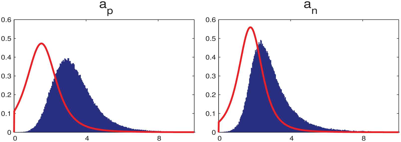
Prior and posterior distributions of the coefficients in matrix $\mathbf{A}$ .

3.3.1. How Do Emissions and GDP Respond to PC and NC Shocks?

Figure 3a displays the cumulative posterior median IRFs of emissions and output along with the 68 percent and 95 percent posterior credibility sets. Stock and Watson (2016) recommend normalizing impulse responses on an economic variable of interest since the scale of the estimated shocks has no economic interpretation. We choose to normalize the size of PC and NC shocks to reduce total emissions by 1 percent on impact by selecting the draw-specific values $-({\hat{a}}_p^{\left(l\right)}+{\hat{a}}_n^{\left(l\right)})/{\hat{a}}_p^{\left(l\right)}$ and $({\hat{a}}_p^{\left(l\right)}+{\hat{a}}_n^{\left(l\right)})/{\hat{a}}_n^{\left(l\right)}$ for each posterior draw $l=1,\dots ,N$ . The resulting impact responses of GDP, $-1/{\hat{a}}_p^{\left(l\right)}$ and $1/{\hat{a}}_n^{\left(l\right)}$ , are inversely related to the histograms of the parameter estimates in Figure 2. Normalizing the shock size on emissions responses will help us compare the magnitude of emissions and energy use responses of different energy users with the responses of total emissions in Section 4.

Figure 3.

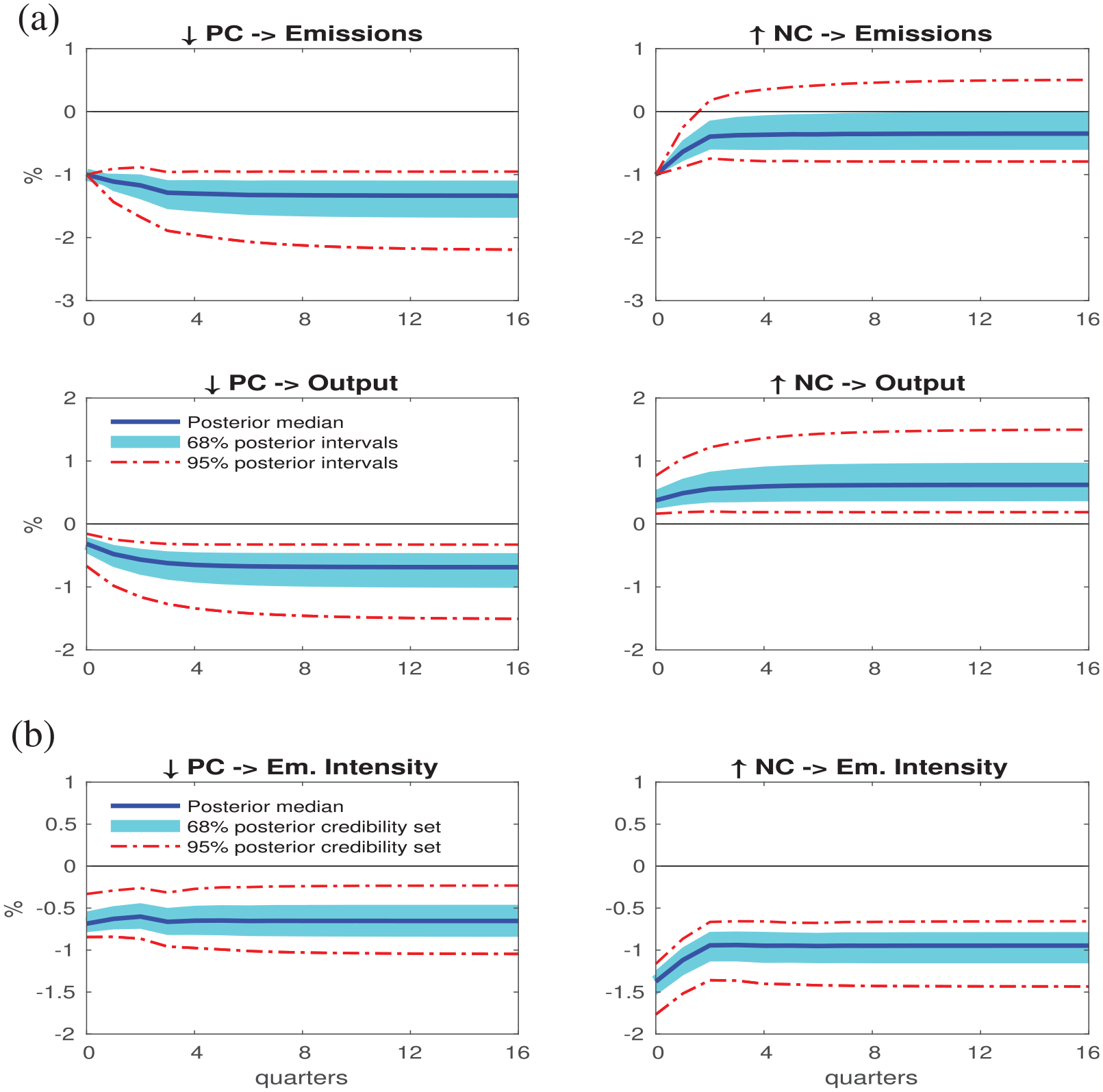
Cumulative responses of GDP, emissions and emissions intensity (VAR). (a) GDP and emissions and (b) Emissions intensity.

The effects of both shocks in Figure 3a are persistent. Even though our identification restricts the impact responses only, the IRF signs extend to other forecast horizons. The median responses and the 68 percent credibility sets show that emissions decline and GDP increases after a positive NC shock, while both variables fall after a negative PC shock. Both shocks reduce the emissions intensity, defined as the ratio of emissions to GDP. Nonetheless, for the same initial 1 percent decline in total emissions, a positive NC shock has a larger impact on the median emissions intensity in all forecast horizons in Figure 3b. ¹⁵

3.3.2. Historical Shock Realizations

Figure 4 plots the median PC and NC shocks. The series start in 1974:Q2 since our VAR includes four lags of the growth rates. The circles mark the quarters for which all estimated shock values within the 95 percent posterior confidence sets have the same signs. The multiplicity of such quarters indicates that the shocks are estimated with high confidence. Another point to note is that all NBER recessions contain large (exceeding one standard deviation) negative realizations of the PC shock while the median NC shock does not follow a clear cyclical pattern. These results suggest that the NC shock may have emissions-specific determinants unrelated to conventional macroeconomic shocks.

Figure 4.

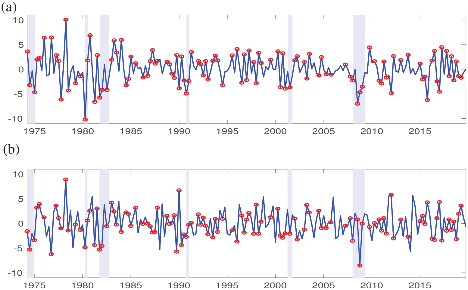
Historical estimates of the sign-identified VAR shocks. (a) PC shock and (b) NC shock.

We use the median NC and PC shocks in the rest of the paper to estimate their effects on U.S. variables. These median shock estimates are robust to several alternative bivariate VAR setups, reported in Section 3 of the online Appendix (different priors, the use of the posterior mean estimates, additional lags, and a longer sample). In fact, all correlation coefficients between the baseline and the alternative shock estimates exceed .92. We next establish that our bivariate VAR is informationally sufficient for the median NC shock.

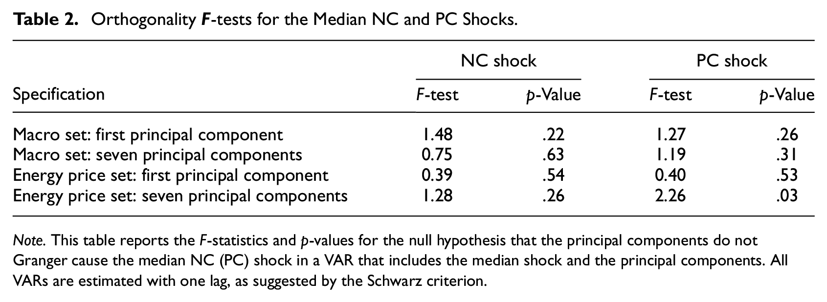
3.4. Testing for Orthogonality of the Estimated Median Shocks

A bivariate VAR parsimoniously summarizes the joint dynamics of emissions and GDP. However, a potential concern is that it may be missing information pertinent to identification. We assess the implications of low dimensionality by conducting a “structuralness” test proposed by Forni and Gambetti (2014). These authors advocate that if a particular shock, estimated within a VAR, is structural, it cannot be Granger-caused (or predicted) by any variables summarizing the state of the economy. ¹⁶ We conduct the orthogonality tests using supplementary VAR models that include the median NC shock (or the median PC shock) and the principal components estimated from a macroeconomic database of 246 U.S. quarterly series maintained by McCracken and Ng. ¹⁷ The orthogonality test corresponds to an $F$ -test for the joint significance of the lagged principal components in the NC (PC) shock equation (Section 2.3.1 in Lütkepohl 1991).

Table 2 reports the results of the orthogonality tests for the VARs using only the first principal component and seven principal components, with the $I{C}_{p2}$ information criterion of Bai and Ng (2002) suggesting seven principal components for McCracken and Ng’s database. The $p$ -values exceed the conventional thresholds for both the NC and PC shocks, supporting the null hypothesis that the macroeconomic factors do not Granger-cause our median shocks. No Granger causality also holds when the number of the principal components included in a VAR varies from two to six, or the number of lags is increased to four.

Table 2.

Orthogonality $\mathit{F}$ -tests for the Median NC and PC Shocks.

Specification	NC shock		PC shock
	$F$ -test	$p$ -Value	$F$ -test	$p$ -Value
Macro set: first principal component	1.48	.22	1.27	.26
Macro set: seven principal components	0.75	.63	1.19	.31
Energy price set: first principal component	0.39	.54	0.40	.53
Energy price set: seven principal components	1.28	.26	2.26	.03

Note. This table reports the $F$ -statistics and $p$ -values for the null hypothesis that the principal components do not Granger cause the median NC (PC) shock in a VAR that includes the median shock and the principal components. All VARs are estimated with one lag, as suggested by the Schwarz criterion.

While McCracken and Ng’s database has extensive coverage of the U.S. macroeconomic and financial variables, it limits the energy-related indicators to the index of industrial production of fuels and the West Texas Intermediate spot oil price. To evaluate the implications of omitting energy prices from our baseline VAR, we extend the orthogonality test of the median shocks to a panel of twenty-five real energy prices, disaggregated by energy types and energy users. ¹⁸ Table 2 indicates that the orthogonality of the median PC shock to energy prices is rejected at the 5 percent significance level in a VAR with seven principal components of energy prices. However, we cannot reject the null of no Granger causality for the median NC shock.

We further test for the orthogonality of the median NC shock to the estimates of prominent macroeconomic shocks assembled from the existing literature. Our list includes news and unexpected shocks to neutral and investment-specific technology, monetary policy shocks, shocks to government spending and taxes, uncertainty and financial market shocks, and shocks to global oil supply and demand (thirty-three series in total). We do not contest the identification of these macroeconomic shocks and treat them as external exogenous variables. The test results, reported in Section 4 of the online Appendix, reveal no predictability of the NC shock.

In summary, we find no evidence that the median NC shock fails to be orthogonal to the past information. Thus, we treat our VAR as informationally sufficient, as defined by Forni and Gambetti (2014), for this shock. ¹⁹ We proceed with analyzing if the NC shock captures CRT innovations and estimate its impacts on macroeconomic and environmental variables.

4. Transmission of the NC Shock to Energy Users

This section extends our analysis to different energy users by employing distributed lag models (DLMs). We find that the NC shock has demand-type effects on the U.S. energy market and that its impact is the most pronounced in the residential and commercial sectors.

4.1. Inference With Distributed Lag Models

Distributed lag models provide a uniform way to estimate the responses of a large number of variables to the NC shock without adjusting the minimal set of VAR restrictions that define them. Each DLM projects the growth rate of a variable of interest, $\mathrm{\Delta }{z}_t$ , on the current and past realizations of the historical shocks from the VAR and includes a constant, as in

$$\mathrm{\Delta }{z}_t={\alpha }_z+\sum _{j=0}^k{\beta }_{\mathrm{zj}}{\hat{\epsilon }}_{t-j}^{\mathrm{nc}}+\sum _{j=0}^k{\gamma }_{\mathrm{zj}}{\hat{\epsilon }}_{t-j}^{\mathrm{pc}}+e_{\mathrm{zt}},k>0.$$

(3)

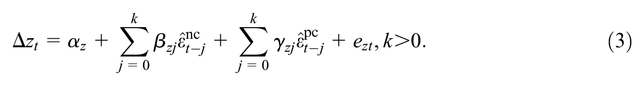
The regression coefficient ${\beta }_{\mathrm{zj}}$ defines the response of $\mathrm{\Delta }{z}_t$ observed $j$ periods after a unitary NC shock. The cumulative response of $z_t$ (in log-level) at the horizon $h$ is the sum of these regression coefficients from the impact period $t$ to $t+h$ . The resulting IRF estimates are entirely data-driven because we do not impose any restrictions on the coefficients ${\beta }_{\mathrm{zj}}$ and ${\gamma }_{\mathrm{zj}}$ .

The DLM results are obtained with the median NC and PC shocks. ²⁰ These shocks are treated as exogenous in (3), and the model is estimated by ordinary least squares. As in Section 3, we set the shock size to reduce total emissions by 1 percent in the baseline VAR (1). Computed at the median parameter estimates, the size of the NC shock is $(\widehat{a_p}+\widehat{a_n})/\widehat{a_n}=2.1920$ . For comparability and ease of interpretation, we keep the same number of lags for all variables: $k$  = 12 for the quarterly data and $k$  = 3 for the annual. We compute standard errors using a block bootstrap procedure that corrects for possible serial correlation in the error term $e_{\mathrm{zt}}$ . All reported results are based on 20,000 replications and a block size of four, as in Kilian (2009).

4.2. Heterogeneity in the Emissions Responses by Energy Users

EIA breaks the U.S. economy into the residential, commercial, industrial, and transportation sectors. These four energy end-use sectors differ in their principal usage and main sources of energy and emissions (EIA 2020). It is, therefore, important to establish if the responses of sectoral emissions to the NC shock conform to those of total emissions.

Figure 5 reveals an intriguing pattern across energy-use sectors. A positive NC shock induces significant and prolonged emissions reductions in the residential and commercial sectors. The residential sector reacts the most, with a −2.66 percent decline. The NC shock has a minimal impact on industrial emissions, with a slight initial decline in the impact period. Emissions in the transportation sector increase, contrary to the fall in the total emissions in the VAR. As we discuss next, the sectoral pattern is robust to controlling for weather effects and using an alternative approach to estimate impulse response functions.

Figure 5.

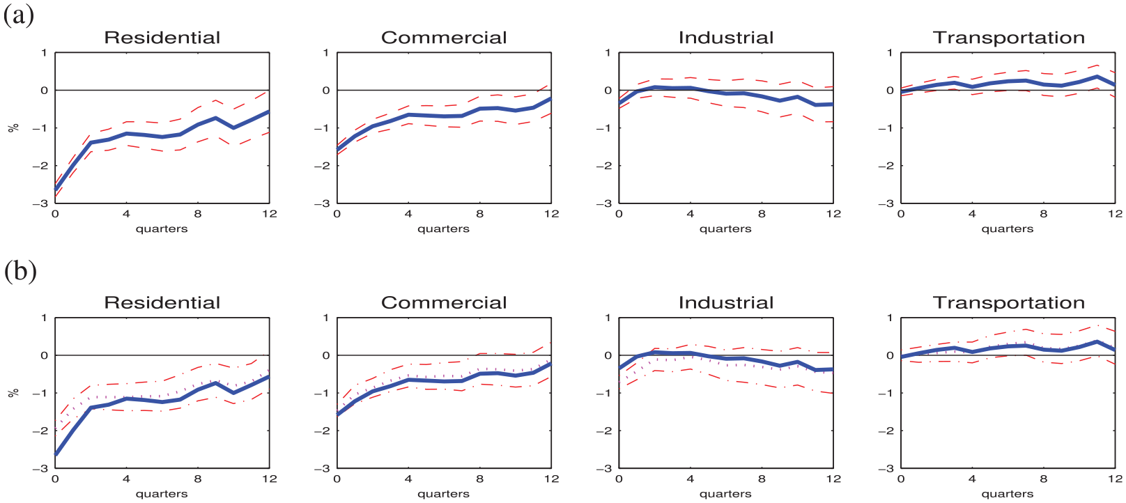
Total energy CO₂ emissions by the end-use sectors (↑ NC, DLM). (a) Total energy CO₂ emissions and (b) Total energy CO₂ emissions, controlling for weather indicators.

4.2.1. Controlling for Weather Effects

Temperature variations directly affect energy demand for heating and cooling and, hence, emissions. However, the impact of weather extremes on emissions and economic activity extends beyond these direct effects (e.g., Dell, Jones and Olken 2014). To assess the implications for our results, we re-estimate the IRFs of emissions using a DLM (3) augmented with the weather-related controls. We use three indicators: the U.S. national average temperature, the residential energy demand temperature index (REDTI), and precipitation. REDTI is shown to be positively related to household energy demand. Precipitation determines the degree of humidity, which, in turn, affects the perceived temperature and influences human tolerance to heat and cold. All three indicators are based on the monthly series from the National Oceanic and Atmospheric Administration. We use the quarterly averages of the deviations from month-specific trends of these series, as detailed in the online Appendix. The augmented DLM includes the current values and four lags of the three weather indicators but keeps twelve lags of the median shocks.

Figure 5b plots the responses of emissions to a positive NC shock from the augmented DLMs and reproduces the IRFs from Figure 5a. Weather variations have the strongest effect on the residential sector, especially in the initial period. This result is not surprising, given that more than half of total energy consumption in the residential sector goes to space heating and cooling and that temperature impacts on the energy demand for cooling and heating tend to be short-lived. Still, the emissions responses in the residential sector remain negative, persistent and significant.

Including the weather controls in the DLMs does not change the pattern of emissions responses. With or without weather indicators, the NC shock is mostly linked to the residential and commercial sectors. Thus we will keep reporting the IRFs based on equation (3).

4.2.2. Accounting for Model Uncertainty

Estimating impulse responses with DLMs is subject to three types of uncertainty: the VAR parameter estimation uncertainty, the VAR model identification uncertainty and the DLM parameter uncertainty. There is no clear guidance in the literature on how to address these three uncertainty types simultaneously. Our main DLM results incorporate the parameter uncertainty embedded in equation (3) but do not account for the shock estimates being generated regressors.

We estimate alternative IRFs based on the entire distribution of historical shocks. This alternative approach takes into account the estimation and model uncertainty of the VAR but abstracts from the DLM estimation uncertainty. Section 3.2 in the online Appendix compares the two sets of responses. In our application, the resulting point IRF estimates are very similar but the implied degree of statistical uncertainty about these estimates is higher in our main DLM specification. We, therefore, follow the approach described in Section 4.1.

4.3. Energy Consumption and Price Responses

The joint analysis of IRFs of energy consumption and prices is informative about the economic nature of the NC shock. Figure 6a focuses on the economy-wide statistics. Total energy consumption declines after a positive NC shock. Despite weakening in the second and third quarters, this response stabilizes around −0.4 percent. Figure 6a also shows that the dynamics of total energy consumption are primarily driven by fossil fuels, while non-fossil energy consumption remains effectively unaffected by the NC shock. The cost of fossil fuel receipts at electric generating plants encompasses the cost of coal, natural gas, and petroleum, including taxes, in producing electricity. ²¹ We use this series as a proxy for the economy-wide energy costs, in the absence of an aggregate energy price. Figure 6a reports a significant 2 percent decline in fossil fuel costs during the first five quarters after a positive NC shock. Considered together, the IRFs in Figures 3a and 6a suggest that the NC shock acts as a negative demand shock for fossil fuels.

Figure 6.

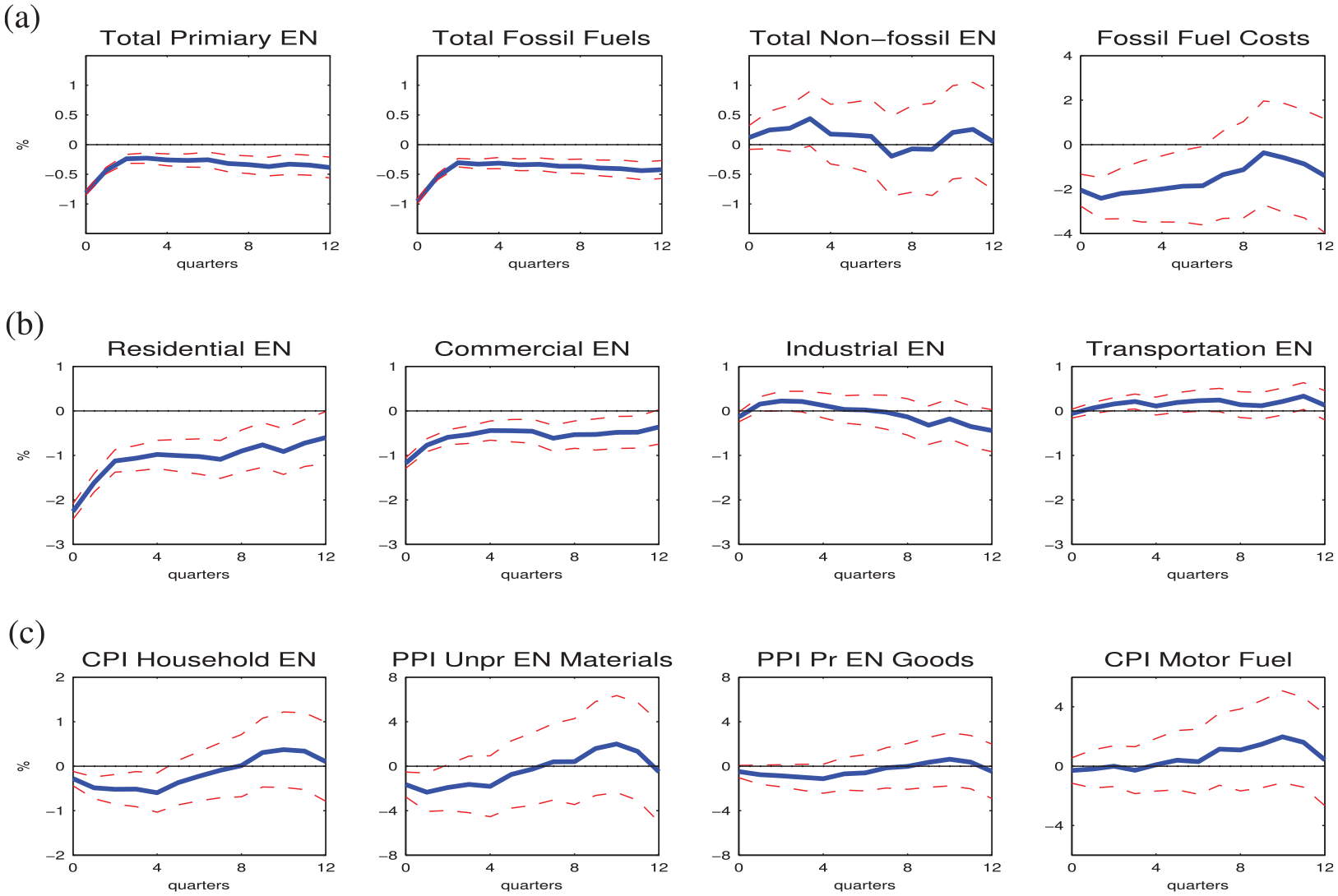
Energy consumption and real energy prices (↑ NC, DLM). (a) Total energy consumption and fossil fuel costs, (b) Total energy consumption, by the end-use sectors, and (c) Selected energy prices.

Figure 6 also provides insights into the NC shock transmission to energy users. We consider several energy prices since energy needs, products, and taxes vary by users. The consumer price index (CPI) for household energy measures the costs of energy expenses for heating, cooling, lighting, and operating appliances and electronic devices. Industrial needs vary from employing energy products as direct production inputs to utilizing electricity to run machinery and equipment. We include the producer price index (PPI) for unprocessed energy materials and processed energy goods as indicators of intermediate input costs. The final energy price, the CPI for motor fuel, is relevant for the transportation sector, a heavy user of motor gasoline.

Energy consumption responses to a positive NC shock in Figure 6b are similar to those of emissions. Price responses in Figure 6c exhibit some heterogeneity. The CPI for household energy declines significantly during the first year. Intermediate energy input costs drop as well, although their responses are more short-lived and less precisely estimated. The response of motor fuel costs is not statistically significant. Overall, the IRFs for different energy users show that the NC shock has the most pronounced impact in the residential and commercial sectors. These sectors seem to experience the NC shock as a predominantly energy demand-reducing shock.

We next assess whether the NC shock reflects CRT innovations, drawing on the economy-wide and sectoral results depicted in Figures 5 and 6 and predictions from general equilibrium models.

5. Explorations into the Economic Meaning of the NC Shock

As discussed in Section 2, general equilibrium models disagree about the macroeconomic effects of CRT innovations. In this section, we revisit theoretical models, focusing exclusively on specifications where CRT innovations reduce emissions. We identify the distinct characteristics of different CRT innovations and evaluate if our NC shock shares these characteristics. We structure our discussion around three categories of CRT innovations: price-induced, policy-induced, and autonomous.

5.1. Energy Price-induced CRT Innovations

An increase in energy costs should provide incentives to develop and adapt new carbon-reducing technologies. This hypothesis is embedded in several classes of micro-founded general equilibrium models, including putty-clay models of energy use (e.g., Kehoe and Atkeson 1999; Wei 2003) and endogenous R&D (e.g., Hassler, Krusell and Olovsson 2021; Fried 2018). We focus on three predictions of models with price-induced CRTs: (i) a negative relationship between emissions and energy costs, (ii) macroeconomic costs of innovation, and (iii) an increased supply of cleaner energy.

First, higher energy costs act as an exogenous trigger for price-induced CRT innovations, reducing emissions. Our NC shock does not operate through this channel. Past energy prices do not predict the NC shock (Table 2). Oil prices can reasonably be argued to align well with the exogeneity assumption. The U.S. is a net importer of crude oil, and oil prices are predetermined with respect to U.S. macroeconomic aggregates (Kilian and Vega 2011). Moreover, the 1973 oil crisis is often cited as a period that spurred the development and adoption of CRT technologies (e.g., Alpanda and Peralta-Alva 2010; Fried 2018). However, a positive NC shock has no significant impact on the PPI for domestic crude oil in Figure 7c or the Refiner Acquisition Cost and the West Texas Intermediate spot crude oil price in Figure 2 of the online Appendix. Additionally, domestic energy prices do not increase after a positive NC shock in Figure 6, and the producer price of natural gas declines persistently in Figure 7b. ²²

Figure 7.

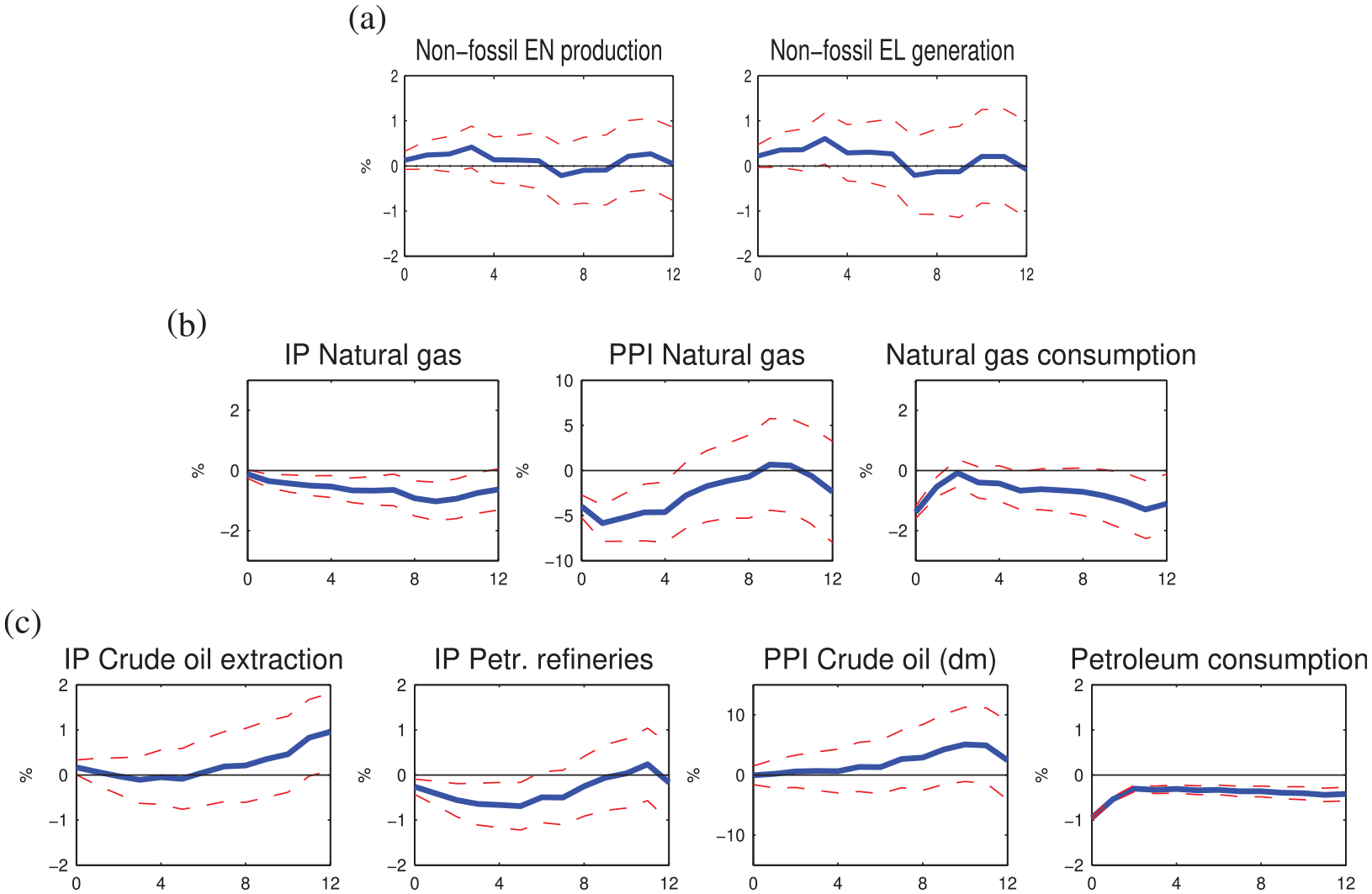
Energy production, consumption, and prices by source (↑ NC, DLM). (a) Clean (non-fossil) energy, (b) Natural gas, and (c) Petroleum.

Second, price-induced CRT innovations can crowd out capital investments and R&D activities in non-energy sectors and technologies, leading to lower aggregate productivity, investment, and stock prices. Our NC shock is not associated with the macroeconomic costs emphasized in the literature. Table 3 provides a summary of the responses of U.S. variables and reports their immediate and peak effects. ²³ We estimate a significant rise in fixed investment, durable goods consumption, total consumption, the NASDAQ index, and corporate net worth following a positive NC shock. These results imply that the investment cost and stock market valuation cost channels are unlikely to be relevant in this context. To assess the R&D crowding-out channel, we use two non-energy technology measures: the quarterly utilization-adjusted total factor productivity series constructed by John Fernald ²⁴ and the annual labor- and capital-saving technology series from Hassler, Krusell and Olovsson (2021). Both series increase slightly on impact but do not significantly change in other periods.

Table 3.

Transmission of the NC Shock to U.S. Macroeconomic Variables (DLM, ↑ NC).

(a) Responses of macroeconomic aggregates
Variable name	Impact effect, %	Peak effect, %
Consumer durables a	0.89 (0.68, 1.10)	1.76 (1.18, 2.33)
Total consumption a	0.17 (0.13, 0.21)	0.55 (0.41, 0.69)
Total investment a	1.25 (1.05, 1.44)	2.34 (1.95, 2.72)
Average hours worked	0.09 (0.07, 0.11)	0.13 (0.08, 0.17)
Labor productivity	0.28 (0.24, 0.31)	0.28 (0.24, 0.31)
(b) Assessment of possible economic costs of the NC shock
NASDAQ index b	1.43 (0.66, 2.20)	4.26 (0.86, 7.66)
Corporate net worth b	0.11 (−0.03, 0.26)	1.81 (0.80, 2.82)
Utiliz.-adjusted TFP	0.15 (0.08, 0.22)	0.15 (0.08, 0.22)
HKO-A (annual)	0.12 (0.03, 0.22)	0.12 (0.03, 0.22)

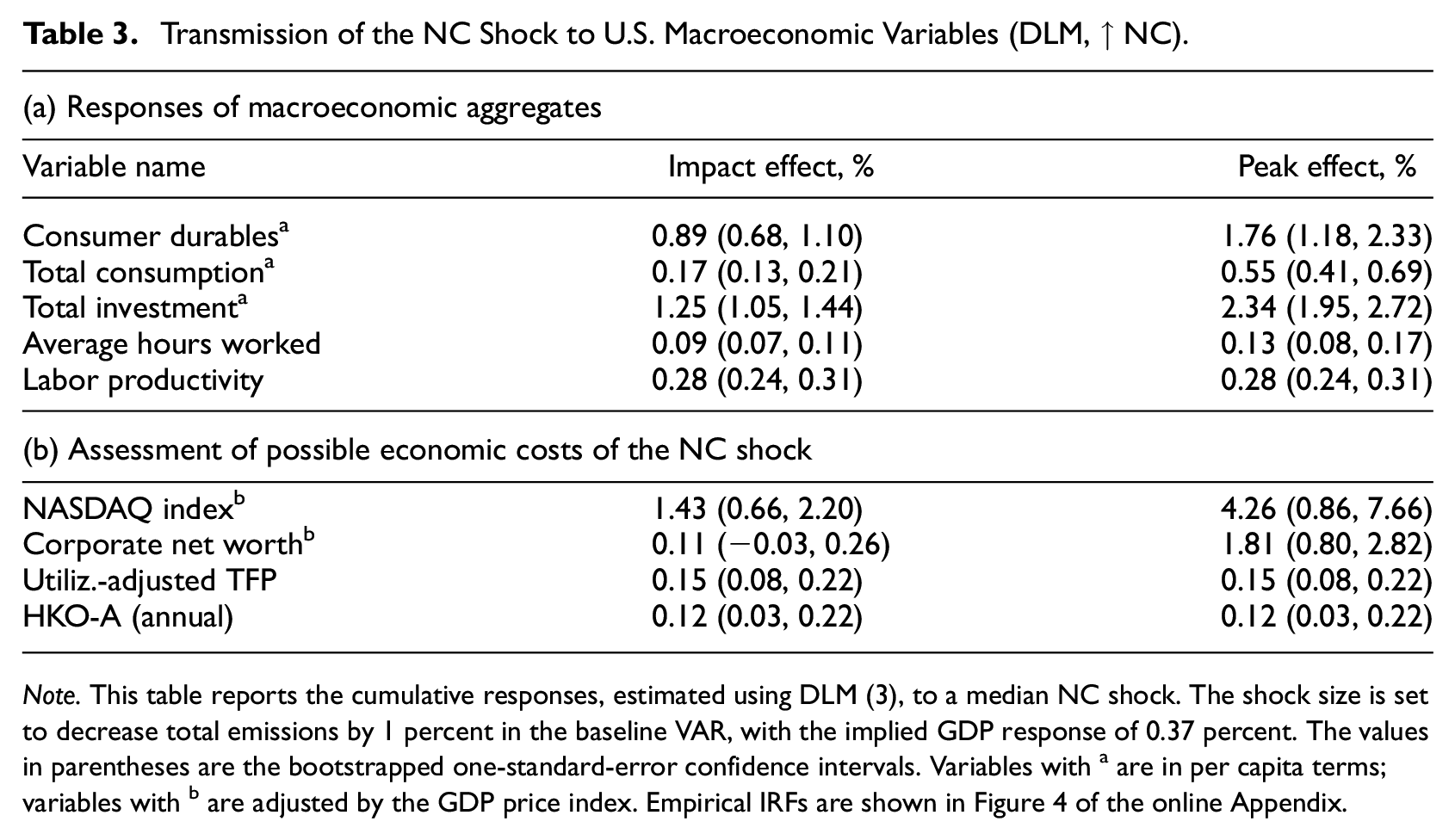
Note. This table reports the cumulative responses, estimated using DLM (3), to a median NC shock. The shock size is set to decrease total emissions by 1 percent in the baseline VAR, with the implied GDP response of 0.37 percent. The values in parentheses are the bootstrapped one-standard-error confidence intervals. Variables with ^a are in per capita terms; variables with ^b are adjusted by the GDP price index. Empirical IRFs are shown in Figure 4 of the online Appendix.

The last prediction is related to CRT innovations in cleaner energy production. Such innovations should increase the supply of carbon-free energy or cleaner fuels. Our NC shock is not transmitted to energy producers according to this prediction. Figure 7a shows that the U.S. production of clean energy and electricity remains essentially unaffected by a positive NC shock. Domestic production of natural gas and petroleum declines in panels (b) and (c) of Figure 7.

In summary, the evidence presented in this section—including the absence of changes in oil prices, a decline in other energy prices, and an increase in investment, stock market prices, corporate profitability, and productivity following a positive NC shock—raises doubts that the NC shock operates through the channels typically associated with price-induced CRT innovations.

5.2. Policy-induced CRT Innovations

Environmental externalities and knowledge spillovers often prevent CRT innovation from reaching socially optimal levels. In addition, informational barriers and substantial upfront costs of adopting new technologies slow their technological diffusion. Consequently, government intervention is widely considered critical to overcoming these challenges. This intervention can take various forms, each tailored to address specific barriers or promote innovation. For example, public R&D funding, such as subsidies, research grants or public-private partnerships, can directly influence the development of new CRTs. Pricing mechanisms, information disclosures, and behavioral incentives can target the adoption of better technologies. Environmental and energy-efficiency regulation can incentivize technological innovation, as hypothesized by Porter (1991).

The Organisation for Economic Co-operation and Development (OECD) attempts to capture the complexity of government policies through its Environmental Policy Stringency (EPS) index. This composite EPS index combines market-based and non-market-based policy instruments designed to mitigate climate change and air pollution, and integrates technology support policies. The annual EPS series for the OECD countries are available from 1990. Albrizio, Kozluk and Zipperer (2017) and Martínez-Zarzoso, Bengochea-Morancho and Morales-Lage (2019) demonstrate that stricter environmental policies, corresponding to higher values of the EPS indices, promote R&D activities, increase the number of patents, and stimulate productivity growth in the OECD economies.

Our NC shock exhibits no relationship with U.S. environmental policies reflected in the U.S. EPS index. Table 4 shows that the NC shock is uncorrelated with contemporaneous changes in the EPS index, or its market-based and non-market-based components. The NC shock also has no significant relationship with current changes in low-carbon R&D spending, U.S. policies promoting technological innovation, or measures supporting wind and solar energy development. Furthermore, the U.S. EPS index and its subcomponents lack predictive power to forecast future values of the NC shock, as demonstrated by the results of the Granger causality tests in Table 4. ²⁵

Table 4.

Climate Policies and the NC Shock (1991–2019).

Regulatory measure	Correlation		Orthogonality
	Coeff.	[Conf.interval]	$F$ -test	$p$ -Value
All environmental policies (EPS index)	−.07	[−.36, .23]	1.16	.29
Market based policies	.26	[−.17, .55]	0.09	.76
Non-market based policies	−.17	[−.41, .05]	0.17	.68
Low-carbon R&D expenditures	.01	[−.47, .35]	1.50	.23
Technology support policies	−.02	[−.42, .32]	1.92	.17
Wind energy support	−.03	[−.33, .10]	0.29	.59
Solar energy support	−.07	[−.27, .09]	1.31	.26

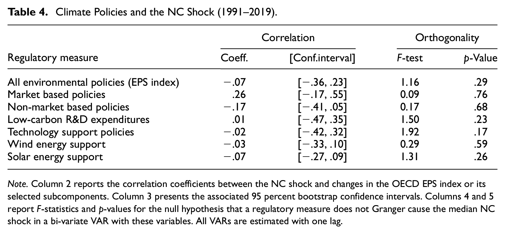
Note. Column 2 reports the correlation coefficients between the NC shock and changes in the OECD EPS index or its selected subcomponents. Column 3 presents the associated 95 percent bootstrap confidence intervals. Columns 4 and 5 report $F$ -statistics and $p$ -values for the null hypothesis that a regulatory measure does not Granger cause the median NC shock in a bi-variate VAR with these variables. All VARs are estimated with one lag.

The main advantage of the EPS indices lies in their comparability across countries and over time. To ensure this comparability, the OECD limits its focus to thirteen policy instruments commonly available across forty countries. As a result, while the composite EPS index provides a comprehensive measure, its coverage of government policies and interventions related to CO₂ emissions remains limited (Kruse et al. 2022). Specifically, the U.S. EPS index does not account for U.S.-specific policies and environmental initiatives implemented at the regional or municipal levels. Furthermore, it does not encompass regulations across all sectors of the economy. Without direct measures of these interventions, we cannot exclude the possibility of their relationship to the NC shock. We revisit this issue at the end of Section 5.4.

Large-scale carbon capture and storage projects, which require substantial upfront investments, represent another critical area for government intervention and public funding. CCS technologies are essential for addressing emissions that are technically difficult to eliminate, such as those from the cement, steel, and chemicals industries. They also support low-carbon hydrogen production and reduce emissions from existing fuel-based power plants through retrofitting. Despite these advantages, the number of large-scale CCS projects and their contribution to emissions mitigation remain low (IEA 2020). ²⁶ In the U.S., the joint carbon capture capacity of CCS projects in 2017 was 24.9 million metric tons of CO₂ (MtCO₂), which is less than 0.5 percent of the total 5,131 MtCO₂ emitted by the U.S. that year. ²⁷ In addition, the net impact of CCS on emissions remains uncertain, as nearly all U.S. operating CCS facilities use captured CO₂ to enhance oil recovery by injecting it into oil and gas reservoirs. The limited and uncertain impact of CCS technologies on U.S. emissions make them an unlikely candidate as the leading driver of the NC shock.

5.3. Autonomous CRT Innovations

Building on existing literature, we define autonomous CRT innovations as technological advancements that occur independently of changes in energy prices or regulatory policies. In general equilibrium models, such innovations are treated as exogenous functions of time. Although few CRT innovations are entirely autonomous and costless in practice, the exogeneity assumption can serve as a reasonable approximation when innovation costs and the impact of government regulations are small relative to the overall size of the economy. Moreover, empirical research on energy efficiency indicates that some EE improvements are autonomous. For example, Newell, Jaffe and Stavins (1999) and Sue Wing (2008) show that substantial variations in average energy efficiency and intensity cannot be explained by energy prices or regulatory changes.

The economic impact of an autonomous CRT innovation depends on whether it primarily influences the U.S. energy market through supply-side mechanisms, such as production efficiency or cost reductions in producing cleaner energy, or through demand-side factors, such as improved efficiency in energy usage. We will discuss these distinct transmission channels separately.

5.3.1. CRT Innovations Influencing Energy Supply

Autonomous CRT innovations that enhance production efficiency or reduce energy generation costs will affect energy supply. They may arise from improvements in producing cleaner fossil fuels or generating low-carbon and carbon-free energy. Breakthroughs in hydraulic fracturing, horizontal drilling, three-dimensional seismic imaging, thin-film photovoltaic technologies, and multi-junction solar cells are just a few examples of innovations that can be considered, at least in part, autonomous. An increase in domestic production of cleaner energy is a robust theoretical prediction for the expected economic effects of these types of autonomous CRT innovations. They should also be associated with higher productivity and lower energy prices. By changing the composition of the energy mix, these innovations can reduce the carbon intensity of the economy.

Our DLM analysis raises doubts about the possibility that the NC shock reflects autonomous CRT innovations influencing the U.S. energy market through supply-side mechanisms. Figure 7 indicates that a positive NC shock reduces natural gas extraction, either reduces or leaves petroleum-related production unchanged and has no statistically significant effect on clean energy production. The same shock reduces the price of natural gas and does not affect the price of oil. ²⁸ Taken together, the energy price and output responses reported in Figure 7 appear inconsistent with the primary expected effect of supply-side mechanisms, namely increased cleaner energy production.

Additional evidence comes from analyzing total factor productivity (TFP) data for the U.S. oil and gas extraction sector, provided by the Bureau of Labor Statistics. TFP, commonly used as a proxy for technological progress, shows several large increases between 2006 and 2015, consistent with the shale “revolution.” However, we find no significant relationship between the TFP growth rate and the annual NC shock, as indicated by the correlation coefficient of 0.188, with the standard error of 0.165.

5.3.2. CRT Innovations Influencing Energy Demand

Autonomous CRT innovations that influence the energy market through demand-side mechanisms tend to synchronize changes in energy consumption and prices, causing them to move in the same direction. Energy-efficiency improvements are a natural candidate for such innovations. ²⁹ Although their net theoretical effect on energy use depends on various factors, this section explicitly focuses on innovations that successfully lower energy consumption and emissions without hindering GDP growth. Structural shocks to the energy efficiency of consumer durable goods and productive capital in a DSGE model of Huynh (2016) share these characteristics. We selected this model to illustrate the transmission of structural energy-efficiency shocks. ³⁰ Huyhn’s model provides the foundation for this section’s analysis, while an extended version incorporating emissions is thoroughly discussed in Section 5 of the online Appendix.

A positive NC shock leads to a simultaneous reduction in total fossil fuel consumption and fossil fuel costs, our proxy for the aggregate energy price (Figure 6). ³¹ The same shock increases GDP, by construction. The transmission of the NC shock to U.S. macroeconomic aggregates aligns with the theoretical predictions for the two structural energy-efficiency shocks in the DSGE model of Huynh (2016). These structural energy-efficiency shocks represent energy demand-reducing shocks specific to the energy market. They decrease total energy consumption and put downward pressure on the energy price due to lower energy demand. Both structural energy-efficiency shocks are expansionary within the model economy, resulting in increases in GDP, consumption, investment, employment, and labor productivity. The empirical responses of U.S. macroeconomic aggregates to a positive NC shock in Table 3 mirror the predicted theoretical effects of structural energy-efficiency shocks. This similarity supports the interpretation of the NC shock as potentially reflecting energy-efficiency improvements.

The NC shock’s differential impacts on major energy users, with the strongest effects observed in the residential and commercial sectors, provide important insights into how a shock that reduces emissions without hindering GDP growth propagates through the U.S. economy. Most macroeconomic models cannot account for the observed pattern of responses, as they typically abstract from consumer energy choices or variations in energy requirements across production sectors. The multi-sector DSGE model of Huynh (2016) is a notable exception. In the context of that model, structural shocks to the energy efficiency of consumer durables and productive capital yield distinct predictions for sector-specific energy consumption, despite producing qualitatively similar effects on macroeconomic aggregates. Specifically, the model predicts a sharp decline in household energy consumption and varying intensities in firm energy consumption responses only when the energy-efficiency shock originates in the consumer sector. Spillovers across energy-saving technologies and innovations targeting the energy requirements of specific sources may broaden the range of possible explanations. Exploring these alternatives is deferred to future research, as we have not identified any general equilibrium model that incorporates this degree of disaggregation.

Our further exploration of the economic nature of the NC shock is based on estimating its relationship with several empirical proxies for energy efficiency. Energy intensity, defined as the amount of energy used per unit of output or activity, is the most common energy-efficiency measure. We consider two economy-wide indicators. The ratio of total primary energy consumption to real GDP is easily constructed at the quarterly frequency. However, this popular indicator also reflects behavioral and structural factors, such as changes in the industrial structure, energy mix, weather or demographics. The U.S. energy-intensity index from Tajudeen, Wossink and Banerjee (2018; TWB energy-intensity index) is adjusted for those factors but is reported only annually.

Since energy efficiency and intensity are inversely related, we anticipate a decline in energy-intensity indicators following a positive NC shock. Figure 8a supports this prediction and shows sizable and highly persistent reductions in the energy-to-GDP ratio and the TWB energy-intensity index. Three years after the shock, the IRF point estimates remain nearly one percent below their initial levels. This decline in energy intensity is not entirely driven by higher output, as evidenced by a reduction in total primary energy consumption in Figure 6a.

Figure 8.

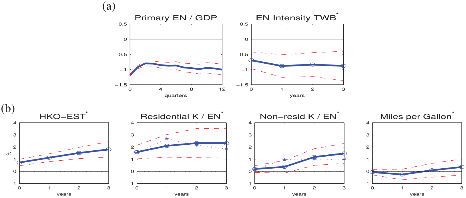
Energy-efficiency proxies (↑ NC, DLM). (a) Measured energy intensity and (b) Annual proxies for energy-saving technology and fuel efficiency.

Figure 8b reports the effects of a positive NC shock on alternative annual proxies for energy efficiency. An energy-saving technology series from Hassler, Krusell and Olovsson (2021), labeled HKO-EST, is derived from a postulated aggregate production function and the U.S. input-output data. Capital-to-energy ratios are informative about energy efficiency when capital and energy services are highly complementary in production or consumption. ³² We construct capital-to-energy ratios for the residential and non-residential sectors, using EIA’s energy consumption series and the estimates of the net stocks of fixed assets and consumer durable goods published by BEA. We also adjust the capital-to-energy ratios for variable capital utilization. Finally, fuel efficiency is measured by miles per gallon for all motor vehicles and reported by EIA. The online Appendix contains detailed descriptions of each energy-efficiency proxy used in the analysis.

If the NC shock captures improvements in energy efficiency, it should be positively related to empirical proxies for energy efficiency. All EE indicators, except fuel efficiency, increase after a positive NC shock in Figure 8b. The impact of the NC shock on sector-specific indicators mirrors the response patterns observed in disaggregated emissions and energy consumption. The capital-to-energy ratio in the residential sector exhibits the strongest response, increasing by more than 1 percent across all reported time horizons. The capital-to-energy ratio in the non-residential sector also increases, albeit only two years after the shock. A positive NC shock does not affect fuel efficiency, as the miles-per-gallon response is insignificant. ³³ This result may be expected, given that total emissions and primary energy use in the transportation sector rise after a positive NC shock (see Section 4). These positive responses contradict the defining characteristics of the NC shock, which reduces total emissions in the main VAR model by construction.

5.4. Challenges Related to Data Measurement

Several data measurement challenges complicate the economic interpretation of the NC shock. First, CO₂ emissions series from EIA are inferred from energy consumption data, rather than measured directly. The conversation from energy consumption to emissions is based on CO₂ emissions factors. Each factor is a fuel-specific coefficient defining the maximum potential CO₂ emissions if all carbon in the fuel is oxidized during combustion. It depends on the density, carbon content, and gross heat of fuel combustion. Reducing an emissions factor would be analogous to operating an industrial carbon dioxide scrubber, a storage technology that absorbs CO₂.

Annual CO₂ emissions factors published by the EIA vary surprisingly little over time. They are constant for 15 out of 36 fossil fuel products throughout the entire sample period, and for all products before 1991. While EIA’s approach produces timely emissions estimates, it may overlook the impact of innovations that reduce the carbon intensity of each fuel. As a result, these emissions series might not adequately reflect the effects of such innovations.

Second, our analysis demonstrates that a positive NC shock is transmitted in the U.S. economy by reducing energy demand. Autonomous energy-efficiency improvements are a possible driving factor. However, shifts in preferences for energy conservation provide a possible alternative. Energy conservation defines behaviors to reduce energy consumption without necessarily decreasing energy services. Monetary costs of conservation behaviors, such as carpooling, air-drying clothes or unplugging idle electronics, are typically low or absent. Gillingham and Stock (2018) find that emissions abatement policies targeting consumers often have low or negative costs. Additionally, Bodenstein, Erceg and Guerrieri (2011) argue that shifts in consumer preferences can justify exogenous energy-saving technology shocks, affecting energy use requirements over time.

Another challenge lies in measuring government interventions. As discussed in section 5.2, the NC shock is independent of the environmental policies captured by the EPS index and its components. However, the policy stringency measures do not encompass all environmental policies. Government interventions promoting energy efficiency and incentivizing energy conservation, which are not covered by the EPS index, are particularly relevant to our analysis.

The U.S. has an extensive system of mandatory and voluntary energy-efficiency standards and employs a variety of non-pricing mechanisms, such as behavioral incentives and information disclosures. Based on their comprehensive reviews of the literature, Gillingham, Newell and Palmer (2006) and Labandeira et al. (2020) conclude that energy-efficiency policies can effectively reduce energy use and emissions. Policy impacts are especially significant for appliance standards and utility-based demand-side management programs in the U.S. residential sector. Newell, Jaffe and Stavins (1999) report a positive effect of stricter standards on average energy efficiency. Moreover, energy-efficiency standards do not seem to have significant adverse effects on manufacturers (e.g., Brucal and Roberts 2019; Jaffe et al. 1995; Nadel 2002). Wiel and McMahon (2003) argue that energy-efficiency standards can be “very effective at limiting energy growth without limiting economic growth,” if they are “designed and implemented well” (Wiel and McMahon 2003, 1405, emphasis in original).

Building on the findings from the previous literature, we hypothesize that energy-efficiency and energy-conservation policies can contribute to explaining variation in the NC shock. The decline in energy-intensity measures in response to a positive NC shock, as shown in Figure 8, along with the reduction in emissions and increase in GDP, can be potentially reconciled with the effects of policy interventions. However, without an explicit measure of energy-efficiency and energy-conservation policies, we cannot draw any definitive conclusions about their relationship with the NC shock.

6. Conclusions

Our research was motivated by the increasing emphasis on technological solutions to combat climate change and the lack of consensus about the effects of CRT innovations on emissions and GDP in theoretical studies. Our literature review revealed that the feasibility of reducing emissions without sacrificing economic growth was debatable in several strands of literature. Combined with the paucity of macroeconomic evidence, the diversity of predictions hindered economists’ ability to inform policymakers about the emissions mitigation potential of CRT innovations. We proposed a novel NC shock, which reduced emissions and increased GDP by construction. This shock exhibits the characteristics of an energy demand-reducing shock, with the strongest impacts observed on emissions and energy consumption in the residential and commercial sectors. CRT innovations that impact the U.S. energy market through supply-side mechanisms, such as production efficiency or cost reductions in cleaner energy, hold the potential to simultaneously reduce emissions and foster economic growth. However, in our sample, these dual benefits do not seem to have materialized.

Our exploratory analysis of the economic interpretation suggests that the NC shock is linked to energy-efficiency improvements, likely stemming from the residential and commercial sectors. There is abundant evidence of energy-efficiency improvements in appliances, lighting, heating, and cooling systems. Technological advancements, such as electric heat pump water heaters, light-emitting diodes (LEDs), loose-fiber insulation, and low-emissivity window coatings, have already led to significant energy savings and hold considerable potential for further savings in the future. ³⁴ Based on our interpretation of the NC shock, energy-efficiency improvements do not appear to reduce GDP. A potential limitation of our methodology is that we are unable to distinguish whether these improvements are exogenous, driven by energy-efficiency or energy-conservation policies, or reflect shifts in preferences for energy conservation.

The urgent need to address the global climate crisis requires a reduction of pollution in all economic sectors. The economy-wide implications of consumer energy decisions remain insufficiently explored in existing literature, and further research is needed to fully understand their economic and environmental impacts. Our findings suggest that focusing on energy-efficiency improvements and conservation in homes could be a viable strategy that promotes both environmental sustainability and economic growth. This strategy would benefit from combining market pricing policies with energy standards, information disclosure, and insights from behavioral sciences (e.g., Allcott and Mullainathan 2010). We align with the perspective of Annicchiarico et al. (2022) that incorporating non-pricing mechanisms, such as energy-efficiency standards, into general equilibrium models would be a promising avenue for research. While mandatory energy-efficiency standards or voluntary labeling programs may be theoretically suboptimal compared to carbon pricing, these policies tend to be more politically feasible and widely accepted.

Our findings also highlight the need to integrate NC-shocks into environmental DSGE models. An accurate representation of empirical drivers of CO₂ emissions in these models is particularly relevant for monetary and fiscal policy analysis. As environmental risks escalate, central banks increasingly incorporate climate considerations into policy frameworks, prompting the development of DSGE models with environmental factors. ³⁵ Since Kelly (2005), it has been understood that the welfare ranking of environmental policies in stochastic environments depends on the mix of macroeconomic shocks. Current models often emphasize traditional shocks that align GDP and emissions, forcing policymakers to trade off between emission mitigation and output stabilization. In contrast, NC-type shocks present no such trade-off, suggesting a path toward policies that balance economic growth and environmental protection. Integrating these shocks into environmental DSGE models can deepen understanding of emission drivers, enabling more effective policy design and reliable evaluation of government interventions.

Supplemental Material

sj-docx-1-enj-10.1177_01956574251322722 – Supplemental material for What Can We Learn About Carbon-reducing Innovations From the Joint Dynamics of CO2 Emissions and GDP?

Supplemental material, sj-docx-1-enj-10.1177_01956574251322722 for What Can We Learn About Carbon-reducing Innovations From the Joint Dynamics of CO2 Emissions and GDP? by Soojin Jo and Lilia Karnizova in The Energy Journal

Supplemental Material

sj-pdf-2-enj-10.1177_01956574251322722 – Supplemental material for What Can We Learn About Carbon-reducing Innovations From the Joint Dynamics of CO2 Emissions and GDP?

Supplemental material, sj-pdf-2-enj-10.1177_01956574251322722 for What Can We Learn About Carbon-reducing Innovations From the Joint Dynamics of CO2 Emissions and GDP? by Soojin Jo and Lilia Karnizova in The Energy Journal