
Abstract
The objective of this paper is to re-examine the causal relationship between oil prices and economic activity for five Asian economies. We apply the unrestricted MIDAS (U-MIDAS) model using monthly data for real oil prices and quarterly data for real GDP for the period from 1998Q1 to 2019Q4. The causal nexus between oil prices and economic activity is also studied by means of wavelet analysis to investigate whether the relationship between the variables changes over different time scales. The key empirical results under the MIDAS approach show that there is a clear significant causal link from oil prices to economic activity, which is not as clearly found under the standard VAR approach. In addition, our results using impulse response functions suggest that the five Asian economies respond, in general, positively in economic activity to an oil price shock at shorter time horizons (less than two years), while the positive responses switch to mostly negative ones at longer time horizons (from two to four years). Our results, in general, support that the (theoretically) expected negative causal nexus between oil price fluctuations and economic activity for oil importers is dominant over longer time horizons for our dataset. An exception to this pattern is China, which has a dissimilar country profile in terms of its oil market and production structure from the profiles of the other Asian economies in the study.
1. Introduction
Since the influential paper by Hamilton (1983), the importance of the world-market price for oil has been well documented in a considerable body of literature in energy economics. Oil price fluctuations and the macroeconomy are also often reported in the news media, so they attract interest from the public, researchers and policy makers. 1 The mechanisms that work as conduits for oil price changes to influence economic activity can be theoretically explained by both supply and demand channels. On the supply side, oil is an important factor for production; thus, an increase in oil prices increases production costs, leading to a decrease in the output of firms. The demand-side explanation is that oil price movements change the purchasing power of oil importers and exporters through wealth transfer effects, influencing consumption and investment. 2 However, an abundant number of studies present mixed findings. For instance, Hamilton (2003) and a recent replication study by Charfeddine, Klein and Walther (2020) using updated datasets show that oil price shocks still have a significant impact on U.S. real GDP growth, but the results in Charfeddine, Klein and Walther (2020) shows that the magnitude of the effect has decreased. Another study by Kilian and Vigfusson (2011) showed a negative impact of oil prices on U.S. real GDP growth. For Asian economies, mixed results also exist. Using Japan as an example, since it is one of the most studied Asian economies, Rebeca and Sánchez (2005) documented no negative real effects of oil prices on economic activity, while Mashi, Peters and Mello (2011) found a negative impact.
Among these numerous studies, we generally note a common feature: a data alignment problem. This means that important economic indicators are released at different frequencies; for example, gross domestic product (GDP) is measured on a quarterly basis, while monthly real oil prices are available using price indexes published on a monthly basis. This data alignment problem is typically handled in such that data reported at different frequencies are aligned at their common lower frequency, resulting in a decrease in the number of observations. This typical remedy, however, might cause potentially useful information to be lost, thereby failing to detect relationships that exist between the variables. Mixed data sampling (MIDAS) regressions were developed by Ghysels, Sinko and Valkanov (2007) to handle situations in which time series differ in sampling frequency. The first MIDAS regression was based on estimating distributed lag models with parameter restrictions, primarily by means of nonlinear least squares. However, for cases where the frequency misalignment is not large, Foroni, Marcellino and Schumacher (2015) introduce the unrestricted MIDAS (U-MIDAS) model without parameter restrictions and use ordinary least squares (OLS) as an estimation method. The current study employs the U-MIDAS model and re-examines the causal nexus between monthly real oil prices and economic activity (which is measured by quarterly real GDP) by fully exploiting potentially useful information. In addition, prior to conducting the empirical analysis using the U-MIDAS framework, we further disaggregate the data into different layers of time scales using the wavelet transform. This approach is based on Ramsey and Lampart (1998), who show that data are aggregated over different time scales and that the time scales should be better specified than in a rough categorization into short and long runs, which is often used in economics and time-series analysis. Moreover, specifying concrete time scales, instead of ambiguously discussing the short and long run, is very useful in policy-making and evaluation processes. This paper, therefore, combines the approaches of Ramsey and Lampart (1998) and Foroni, Marcellino and Schumacher (2015) and introduces a U-MIDAS model using wavelet-transformed data.
Employing a MIDAS model within the wavelet framework is a novel approach to investigating the causal relationship between oil prices and economic activity. Testing for Granger causality in a MIDAS framework was first discussed by Ghysels, Sinko and Valkanov (2007), who noted that causality testing based on temporal aggregated data can have difficulties detecting a significant causal link. 3 The challenge in disaggregating the data is the overparameterization of the model, especially if the difference in frequency is large. Solutions to this issue include nonlinear parameter constraints, as shown in Ghysels (2016). However, when the frequency misalignment is small, Foroni, Marcellino and Schumacher (2015) showed that not imposing any restrictions leads to superior predictive performance. Based on this U-MIDAS framework, Ghysels, Hill and Motegi (2016) suggested a mixed-frequency vector autoregressive (VAR) model and showed that the standard Wald test is consistent. They also showed that testing for causality is more powerful than temporally aggregating the data. In addition, using wavelet-transformed data avoids the problems of nonstationarity and information that is too loosely aggregated over different time scales. The use of a standard causality test based on wavelet-transformed data dates back to Ramsey and Lampart (1998), and implementing different types of Granger causality tests on wavelet-transformed data is an established method (e.g., Benhmad 2012; Tiwari and Albulescu 2016).
Against this backdrop, we revisit the nexus of oil prices and macroeconomic activity for selected Asian economies using a U-MIDAS model with wavelet-transformed data. Our motivations for studying five Asian economies—China, Japan, Korea, Singapore, and Thailand—are twofold. First, these economies have driven regional economic growth in different periods in the past, and they belong to either high-income or upper-middle-income groups 4 according to the World Bank. These countries have had increasing importance in the global economy through their integration into global value chains and the international trading system, and the trade intensity of these economies has grown (WTO and IDE-JETRO, 2011). Hence, understanding the behaviors of these economies, which are situated in one of the fastest-growing regions in the world, with respect to oil price fluctuations is useful. Second, these economies have shown a noticeable increase in fossil fuel consumption over the past few decades (Saboori and Sulaiman 2013). The effects of oil price movements on these economies should, therefore, not be confined to the national domain but may ripple through regional and global economic environments. The macroeconomic performance of an economy in response to oil price shocks, however, is also closely associated with the responses of monetary policy measures, whose transmission mechanism itself influences the exchange rate and oil prices (Natal, 2012). Based on this account, we include the inflation rate, interest rate, and the exchange rate in the empirical model of the current study, following the framework developed by Cunado, Jo and de Gracia (2015) and Karlsson, Månsson and Sjölander (2020), and orthogonalize the variables to focus on the impact of oil price fluctuations. As a robustness check, we also employ the approach of Ghysels, Hill and Motegi (2016) and include the control variables directly in the VAR model.
The main results of the paper are summarized as follows. When we use MIDAS instead of a standard VAR model, the p-values of the causality tests decrease since we gain information by disaggregating the oil prices. The analysis of the impulse-response functions also revealed that the five Asian economies respond positively to an oil price shock at shorter time horizons (less than two years), while the positive responses generally change to mostly a negative direction at longer time scales (from two to four years). Additional accounts of this evidence may cover monetary policy measures, forms of energy contracts, and long-term energy policy. On the other hand, the negative responses of economic activity to an increase in oil prices for most of the economies in the study can also be explained by the cost adjustment mechanism (through supply channels), which generally holds at longer time horizons. An exception to the countries showing this general tendency toward a switch in signs at different time horizons is China. The country shows positive responses in economic activity to oil price shocks across all time horizons (measured in wavelet scales from two quarters to four years). Some explanations may come from the fact that the country has a different profile in the oil market from that of other Asian economies, having its own domestic oil production and refinery capacity. Another distinct case in the study is South Korea, which does not show clear positive responses in production with an increase in oil price at shorter time horizons and presents very small negative responses at longer time horizons.
To our knowledge, this is the first paper to use the MIDAS framework and wavelet analysis for the nexus of oil–economic activity. We show that it is very important to use disaggregated data that show the relationships between these two important macroeconomic variables, which are otherwise masked in the analysis of temporally aggregated data. The relationship between oil prices and economic performance is not deterministic; rather, it is largely driven by a mixture of economic policies, the effects of which might be shown with temporal dynamics. The findings of this study, therefore, add to the literature since they utilize data without losing information when matching the frequencies of observation. In addition, they disentangle the specific relationship between oil prices and economic activity at different time scales.
2. Literature Review
There is extensive research on the oil price–macroeconomy relationship. In this section, we present the studies that we find most relevant to the current study, with a focus on Asian economies.
2.1. Country-Level Analyses
Japan is an Asian economy that was studied earlier than the others (Burbidge and Harrison 1984; Darby 1982). 5 In more recent work, Lee, Lee and Ratti (2001) found that oil price shocks have a significant impact on Japanese output, which is attributable to the monetary tightening induced by oil prices. Rebeca and Sánchez (2005) documented that from 1972:Q1 to 2001:Q4, no negative real effect of oil prices on economic activity in Japan was identifiable in a Granger causality analysis using seven macro indicators, in contrast to their findings for the other economies of a significant negative impact of oil prices on GDP growth. Zhang (2008) reported that nonlinear and asymmetric relationships between oil price shocks affect economic growth in Japan using quarterly data from 1957Q1 to 2006Q4. Hanabusa (2009) found that a change in oil price Granger-causes the mean economic growth rate in Japan, with lags of nine months. Lee and Song (2009) divided their sample period into two subperiods, 1987Q1 to 1997Q4 (precrisis) and 2000Q1 to 2009Q1 (postcrisis), and investigated the responses of the macroeconomic activity of Korea using quarterly data on real GDP, the CPI, exports, and oil prices. The impulse response analysis showed that exports increase due to oil shocks, which was not the case in the precrisis sample. They observed that oil price shocks increased the price level and real interest rate in the postcrisis period. Unlike in the precrisis subsample, adverse negative effects of oil prices on real GDP were found in the postcrisis period. An and Kang (2011) employed a Bayesian estimation framework including a dynamic stochastic general equilibrium-vector autoregression (DSGE-VAR) model using quarterly data on real GDP, core inflation rates, nominal hourly wages, nominal exchange rates, nominal interest rates, and real oil prices for 1993:Q2 to 2008:Q4. They documented that an oil price shock has immediate negative impacts on most macroeconomic indicators; however, it has positive effects in the medium term. Park, Chung and Lee (2011) delved into regional responses within the country using a structural VAR model and showed negative responses to an oil price increase for industrial production and price.
More recently, studies on the oil–Chinese macroeconomy nexus have been conducted. Du, He and Wei (2010) focused mainly on the relationship between oil price shocks and economic growth and inflation based on a monthly time series from 1995:1 to 2008:12 using multivariate vector autoregression. Oil price shocks had significant effects on economic growth and inflation in China, and the relationships were nonlinear. They also reported the exogeneity of the world oil price with respect to macroeconomic activity in China. Zhao et al. (2014) employed a DSGE model to study the effects of different types of oil shocks on output and inflation in China for the period 1990/2013. The results showed that different oil shocks have varying effects on China’s macroeconomic aggregates. By using seven different quarterly macro data series covering 1996:Q1 to 2014:Q4 with a VAR model, Wei and Guo (2016) found that oil price shocks have positive effects on China’s output, mainly due to a rise in exports, while causing negative effects on China’s interest rate. Most recently, Gong and Lin (2018) investigated the time-varying effects of oil supply and demand shocks on the Chinese macroeconomy. They employed a time-varying parameter structural vector autoregression with a stochastic volatility model using monthly reports of world crude oil production, the global real economic activity index, the real oil price, and the price index. The time-varying effects of the different oil shocks on China’s output and inflation were presented over the period from 1995 to 2015.
2.2. Panel Setting with Oil Exporters and Importers
Abeysinghe (2001) used a structural VARX model in which the direct and indirect effects (through exports) of oil prices on GDP growth for 12 economies were investigated. Quarterly data on GDP, bilateral exports and oil prices for the period 1982Q1 to 2000Q2 were used for the ASEAN-4 (Indonesia, Malaysia, the Philippines, Thailand), the NIE-4 (Hong Kong, South Korea, Singapore, Taiwan), China, Japan, the USA, and the remaining OECD as a group (ROECD). The net oil exporters among the ASEAN-4 countries, namely, Indonesia and Malaysia, show a direct impact of high oil prices on GDP growth; however, they also face countereffects in the long term through trading partners. This transmission effect of oil prices on economic growth does not seem to be noticeable for a large economy such as the U.S., but it can be important for small open economies. Cunado and de Gracia (2005) focused only on Asian economies, which are both net oil exporters (Malaysia) and net oil importers (Japan, Singapore, South Korea, the Philippines, and Thailand), to investigate the impact of oil prices on the macroeconomy (economic activity measured by different proxies depending on the data availability of the economies and consumer price indexes) over the period 1975Q1 to 2002Q2. The results suggested that oil prices have a significant short-term effect on both economic activity and price indexes. This effect becomes more significant when oil prices are expressed in local currencies. No evidence of an asymmetric relationship was generally observed, except for South Korea, which has domestic currency–denominated oil prices. Berument, Ceylan and Dogan (2010) focused on MENA countries that are not major oil exporters and used causality tests in a VAR framework. They found statistically significant effects for Algeria, Iran, Iraq, Kuwait, Libya, Oman, Qatar, Syria, and the United Arab Emirates. Ran and Voon (2012) used quarterly data on real GDP, the unemployment rate, the import price, the general price level, the interest rate, oil import consumption, and the nominal world crude oil price index in both recursive VAR/VECM and panel data models to examine the oil–macroeconomy relationship for the Asian small open economies (Hong Kong, Singapore, Taiwan, and South Korea) from 1984Q1 to 2007Q3. There was no evidence of significant impacts of oil price shocks on real GDP in any model specification. Unlike previous studies, they detected contemporaneous effects of oil shocks on the general price level (in panel regressions) and positive significant effects on unemployment with time lags.
2.3. A Comparison of Developing and Developed Economies
Studies on Asian economies about the oil–macroeconomy nexus have also been performed to examine whether they show differences with respect to developed economies. For example, Aastveit, Bjornland and Thorsrud (2012) studied the effects of three different types of oil shocks on thirty-three countries (eighteen developed and fifteen emerging countries) and detected that an oil demand shock caused by global economic activity has a common positive effect on GDP across all regions. An oil supply or an oil-specific demand shock, however, brings about varying responses to economic activity in different regions. More precisely, North American and European countries face an adverse effect from oil supply shocks on economic activity, yet some Asian countries show a positive effect. An oil-specific demand shock affects developed countries in Europe and North America more than emerging countries. These varying effects may be explained by underlying structural changes such as the long-term energy policy of some Asian economies. Taghizadeh-Hesary et al. (2016) studied the oil–macroeconomy (GDP growth rates and inflation rates) nexus of the world’s largest oil consumers, grouped into developed economies (including the U.S. and Japan) and an emerging market, the People’s Republic of China. They argued that oil price fluctuations affect GDP growth more in developed economies than in emerging economies. They also suggested different reasons for the lower influence of swings in oil prices on developed economies than on emerging markets: the degree of fuel substitution for renewables, for example, and energy efficiency policies in developed economies. However, oil price fluctuations had a milder impact on inflation rates in the emerging market than in the two developed economies included in the study.
2.4. Long-Run and Short-Run Responses
Discussions and findings about the long-run and short-run relationships between oil prices and economic activity are often based on the results of the cointegration approach and vector error correction model. Cunado and de Gracia (2005) focused on four of the top oil-consuming Asian economies (Japan, India, Korea, and Indonesia) and reported that the responses of economic activity to an increase in oil price differ depending on the type of oil price shock. The results suggested that oil prices have significant effects on macroeconomic indicators, yet the impacts are limited to the short run. They also reported that an oil supply shock has a limited impact, while a demand shock caused by global economic activity has a significant positive effect on the economies included in the study. Asymmetries and nonlinearity have also been investigated by means of different time-series models. Lardic and Mignon (2008) documented empirical evidence for asymmetric cointegration between oil prices and the GDP of the U.S. economy and Euro area economies: the impact on GDP from an oil price increase is greater than that from an oil price decrease. Khan, Husnain and Abbas (2019) presented, for thirteen selected Asian economies, symmetrical responses of real GDP to oil price changes in both directions, with no long-run asymmetry in any of the economies. More recently, by using the nonlinear autoregressive distributed lag (ARDL) model, Nusair and Olson (2019) showed that oil prices symmetrically affect the real GDP of seven Asian economies both in the short and long runs. Several other recent studies, albeit not about Asian economies, extended the dataset of previous studies to 2019:Q4 and sought to replicate the results (Charfeddine, Klein and Walther 2020). They showed that the explanatory power of the oil price for GDP growth persists; however, the magnitude of the oil price effects on production is slightly weaker when the oil price increases and shows no change in the case of oil price decreases. The MIDAS approach started to be employed in the recent literature on energy economies. For example, Pan et al. (2018) employ the MIDAS approach to predict U.S. GDP using oil prices, while Salisu and Ogbonna (2019) apply the MIDAS regression to model the energy–growth nexus. Zhang and Wang (2019) report that forecasting crude oil prices using higher-frequency data significantly outperforms forecasting based on low-frequency data.
3. Brief Notes on Methodologies
3.1. Wavelet
Wavelet analysis is a method for disaggregating time series data into different layers of time scales. For example, Ghysels, Hill and Motegi (2016), Salisu and Ogbonna (2019), and Charfeddine, Klein and Walther (2020), who analyzed the nexus between oil prices and GDP via the MIDAS approach, have only temporally disaggregated the data. We take this one step further and disaggregate it into different time scales as well. This section provides a brief description of the wavelet and maximum overlap discrete wavelet transformation (MODWT). 6 The version of wavelet decomposition that we utilize in the paper is based on “moving averages of the original data and moving averages of moving averages” (Hacker, Karlsson and Månsson 2014, 323). This approach is more common in the literature (e.g., see Raza et al. 2018) than the discrete wavelet transform (DWT). This is because the decomposition can handle any sample size, lead to a larger sample size for estimating correlation coefficients and regression models, and provide increased resolution at coarser scales. This method decomposes data into J scale levels, producing, at each jth level of the decomposition, a series of averages usually denoted the smooth series (Sj), which consists of averages over values of next-lower scales. Furthermore, a detailed series (Dj) is produced, which contains the differences in the smooth series of the next-lower scale level. The potential depth of the wavelet decomposition (i.e., how large the scale level can be) ultimately depends on the number of observations of the time series. In this paper, we use J = 4 since we have quarterly and monthly data covering twenty-two years (1997–2019). The equations below present formulas for wavelet details (D) and smoothing (S) for each scale level j.
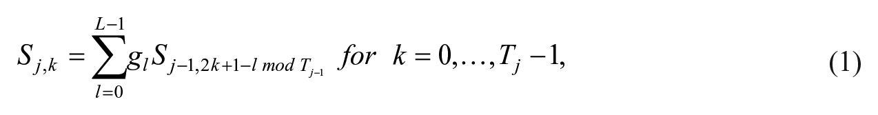
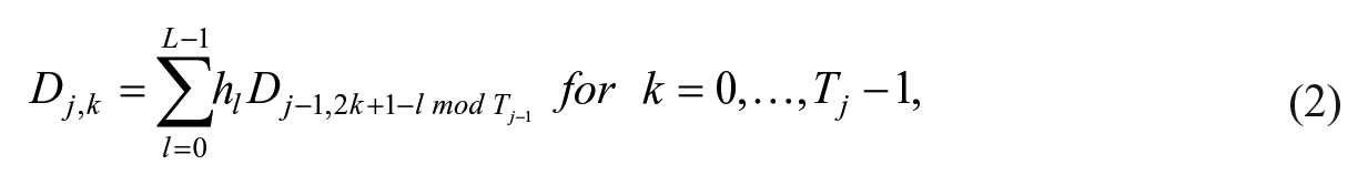
where
3.2. Mixed-Frequency VAR Models
The standard VAR model based on wavelet-transformed data was first introduced by Ramsey and Lampart (1998), which can be written as:
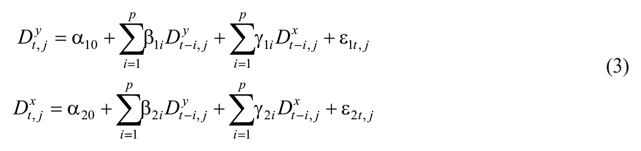
where
The issue with mixing data from different sampling frequencies is that it may lead to overparameterization if the difference in frequency is large (e.g., monthly and daily data). To address this situation, the first paper introducing MIDAS modeling by Ghysels, Santa-Clara and Valkanov (2004) suggested applying distributed lag models that restrict the parameters of the lags to follow a certain pattern, such as an Almon lag or a Beta function, which decreases the number of estimated coefficients. However, Foroni, Marcellino and Schumacher (2015) showed that when the difference in sampling frequency is small, the restricted estimator suggested by Ghysels, Santa-Clara and Valkanov (2004) is not necessary; instead, it is possible to use OLS. This method is not based on parametric restrictions; therefore, the authors coined the term unrestricted MIDAS (U-MIDAS). The choice of this method aligns with previous research in which Ghysels, Hill and Motegi (2016) introduced a causality test based on U-MIDAS when the frequency mismatch is small. The authors also illustrated this method by analyzing the nexus between oil prices and GDP. We generalize the method from Ghysels, Hill and Motegi (2016) in the same way that Ramsey and Lampart (1998) generalized the standard VAR model. Therefore, we estimate the following U-MIDAS model based on wavelet-transformed data:
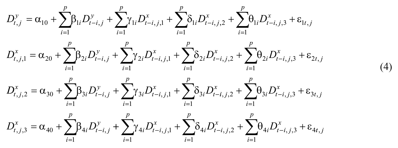
where
4. Data and Preliminaries
In this study, we use monthly real oil prices and quarterly real GDP from 1998Q1 to 2019Q4. 10 The monthly oil prices (WTI spot FOB, dollars per barrel) per barrel were collected from the U.S. Energy Information Administration (EIA) 11 ; then, these prices were converted to real prices by using the U.S. Consumer Price Index. 12 Figure 1 shows that the real crude oil price per barrel in dollars, on a log scale, is associated with economic and geopolitical events, which affect the global economy. More precisely, the Asian financial crisis lagged behind the price decrease in 1998, as shown in Figure 1. The decline in the oil price in 2001 can be explained by slack demand for oil in the global market due to downturns in the U.S. economy and increased uncertainties caused by the 9/11 attack. Figure 1 also shows that there was a general increasing trend in oil prices after 1999. Then, one of the noticeable price decreases is observable between 2008 and 2009. This abrupt and marked fall in oil prices is due to the global financial crisis, which caused demand to plummet in 2008. The figure also shows a more recent price decrease in oil prices from 2014 to 2015. Both the supply and demand factors of the oil market caused the oil price to plummet during this time. While a growing supply glut drove an oil price drop, the sluggish economic situation of the oil-importing economies led to further price decreases in oil due to their decreasing demand for oil.
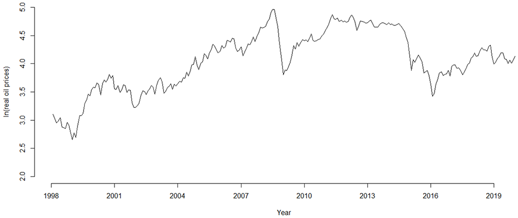
Time plot of real oil prices on a log scale over the sample period.
The quarterly real GDP data are from FRED, Federal Reserve Bank of St. Louise. 13 As an example, the quarterly real GDP of Japan is illustrated in Figure 2. The economy shows a steady increasing trend in domestic production. As commonly observed in most economies, Japan experienced a remarkable drop in production around the years 2008 to 2009 caused by the financial crisis, which hit the global economy hard.
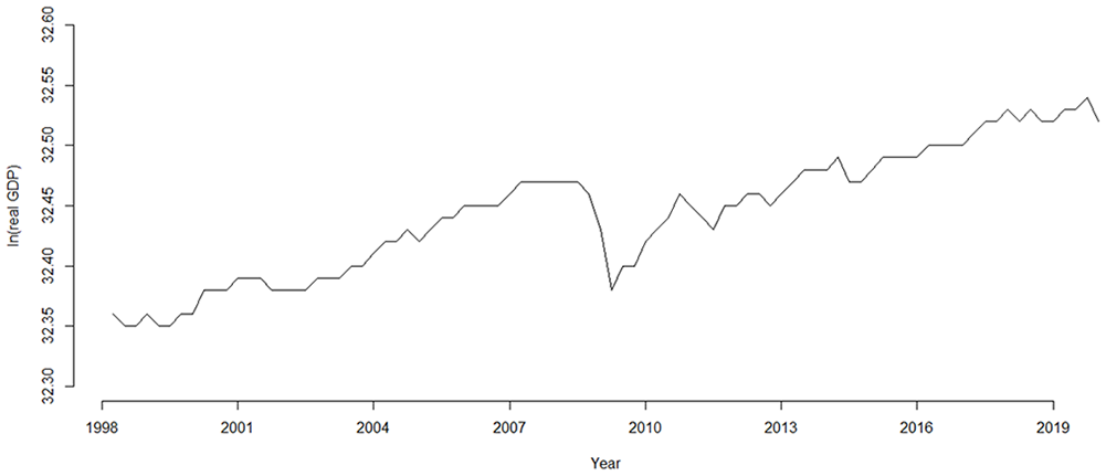
Time plot of the real GDP of Japan on a log scale over the sample period.
Monthly data on nominal interest rates (three-month or ninety-day rates, percent per annum) are also collected from FRED, and the inflation rates are calculated using the consumer price indexes from this database. The monthly real effective exchange rates are obtained from the official website of the Bank of International Settlement (BIS). 14 Interest rates, inflation rates and exchange rates are used in the orthogonalization process to focus on the effects of oil price shocks by removing the transmission mechanism of oil price shocks on the economy through monetary and exchange rate policies. These variables will be used as control variables by applying orthogonalization where the residuals from an OLS model where GDP and oil prices are regressed on the inflation rates, exchange rates, and interest rates. This type of orthogonalization method was used in Hacker, Karlsson and Månsson (2012) as a robustness check to account for other major determinants of the variable of interest. The wavelet transform is performed on the orthogonalized quarterly production data and the monthly real oil prices, with the wavelet details explained in Section 3.1. Then, we wavelet transform them and include them directly in the VAR model. More details can be found in Section 5.
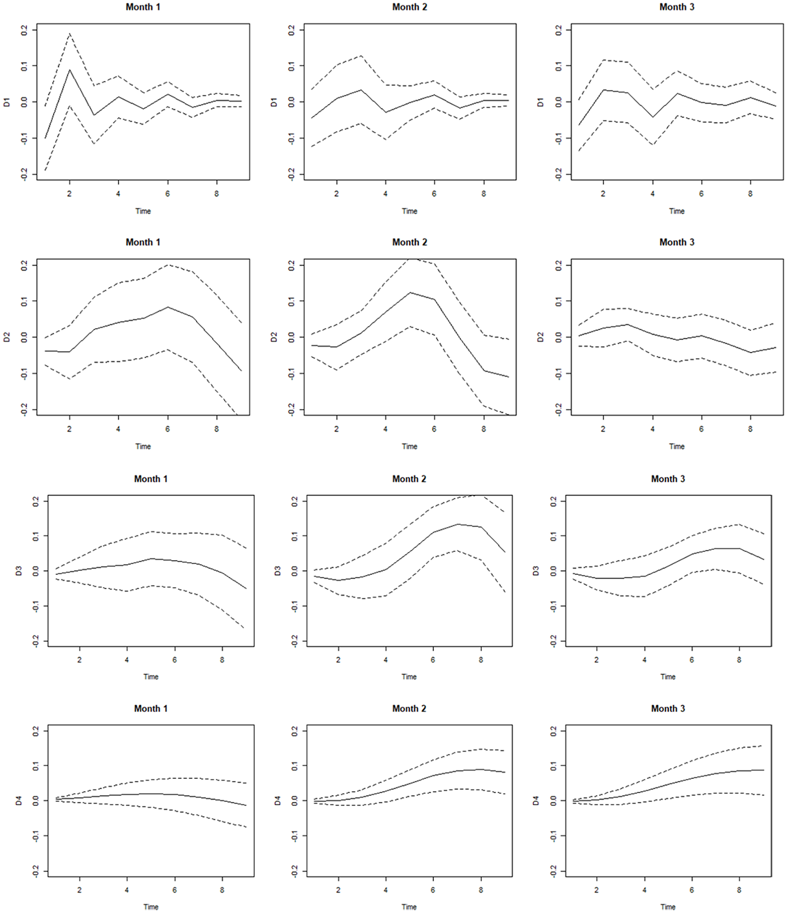
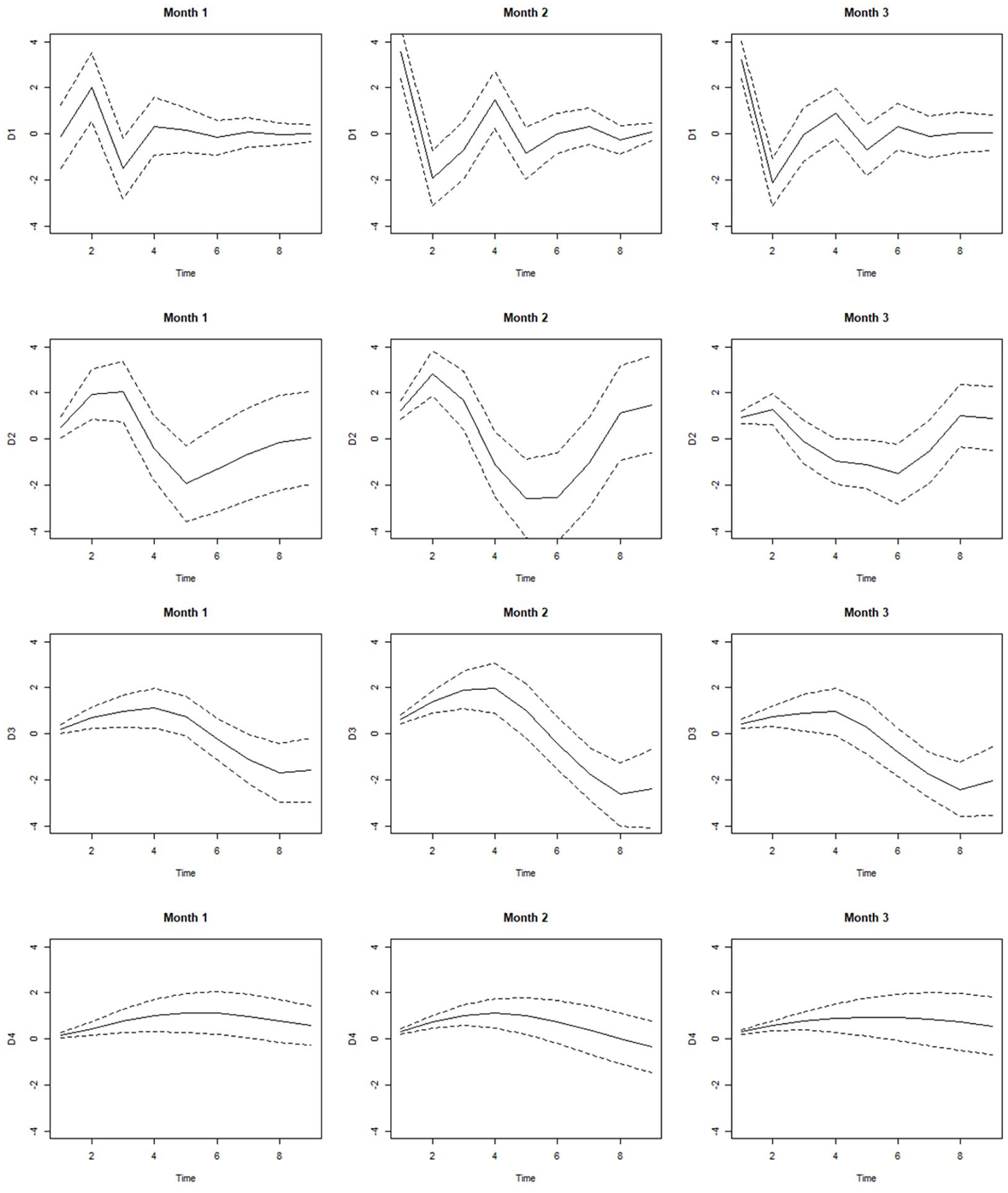
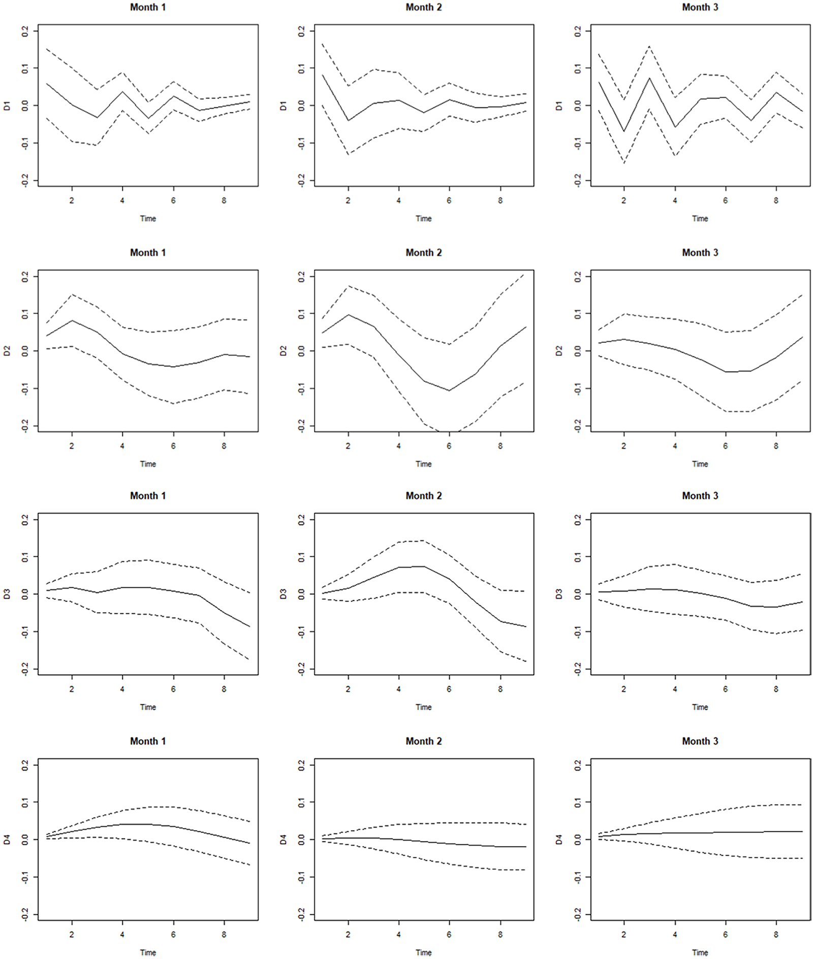
In Table 1, we include descriptive statistics of the wavelet details for real oil prices and GDP. Notably, the standard deviation peaks at D3, which is not expected since the short term is usually more volatile. The kurtosis is also largest for D3, which can be explained by the greater variation, which causes larger deviances from the mean. Figure 3 presents the wavelet details of the real GDP of Japan at different wavelet scales as an example, and Figure 4 shows the wavelet details of the oil price for the third month in each quarter. 15 The Dj label on the vertical axis denotes the wavelet scales associated with the wavelet details. The numbers appended to the wavelet detail notations, J, show the wavelet time scales. In the present paper, the scale levels are constructed such that D1 is associated with one to two quarters, D2 is associated with two to four quarters, D3 is associated with four to eight quarters, and D4 is associated with four to eight quarters.
Descriptive Statistics of the Wavelet Details.

Note. OilM1 is the real oil price for the third month in each quarter (which corresponds to the first lag in the VAR-models), OilM2 is the real oil price for the second month in each quarter, and OilM3 is the real oil price for the first month of each quarter.
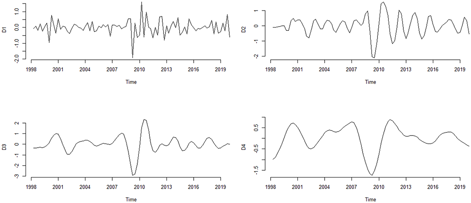
Wavelet details over the GDP of Japan.
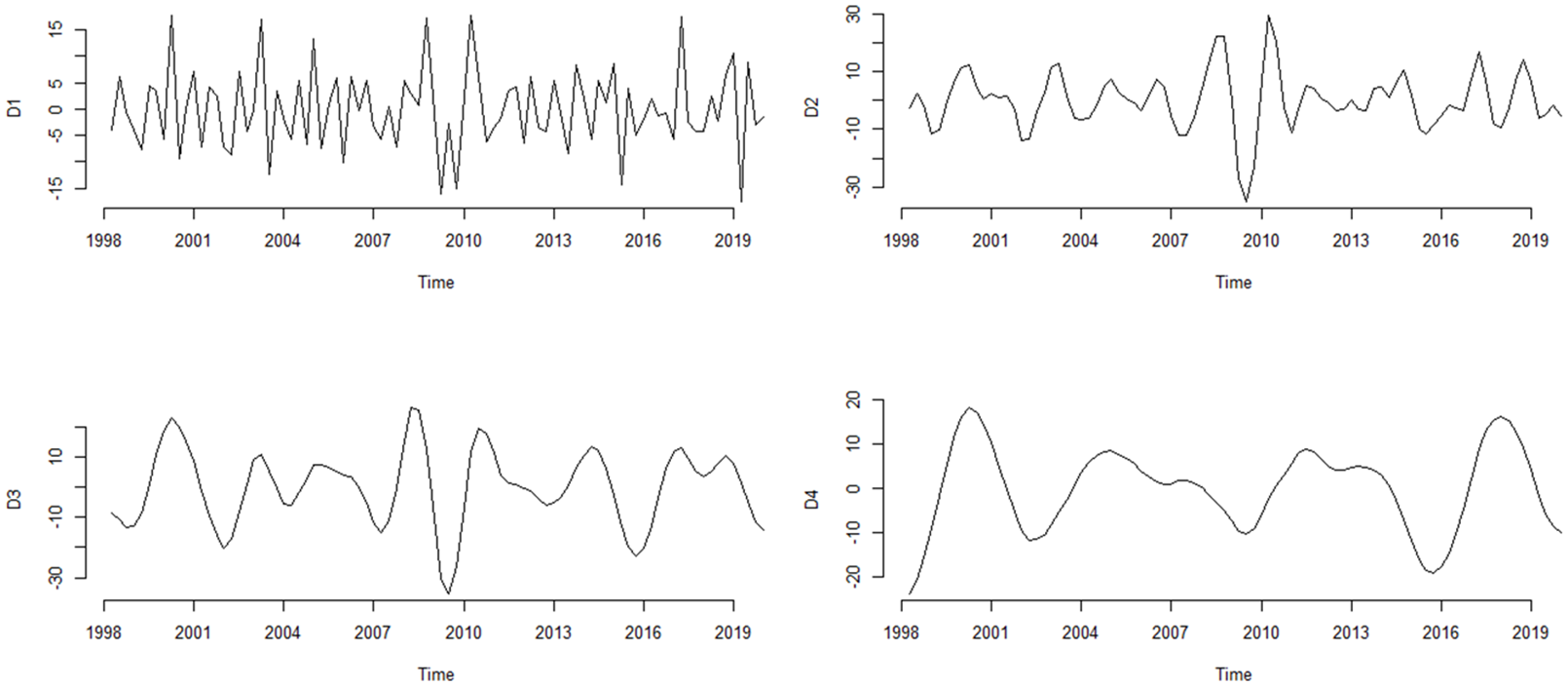
Wavelet details over oil prices for the third month in each quarter.
Our goal is to consider causal relationships in a Granger sense between real oil prices and real GDP, which are collected at different sampling frequencies. The focus of the paper is the causal relationship between oil prices and economic activity 16 for the following two reasons. First, as shown in equation (4), the MIDAS framework suits the causal relationship investigation from real oil prices to production. Second, most of the economies included in the study are not considered individual consumers that have an effect on the global oil market. 17
5. Testing Methodologies
As mentioned in an earlier section, we suggest a novel approach for testing for causality using wavelets in a MIDAS setting. We consider the parametric framework in the same manner as Ghysels, Hill and Motegi (2016). In several papers (Benhmad 2012; Tiwari and Albulescu 2016, among others), different nonparametric (and nonlinear) Granger causality tests in the wavelet domain (both continuous and discrete) have been used. These tests are not yet generalized in the MIDAS framework, and several challenges exist, such as parameter proliferation and how to temporally disaggregate the data for continuous wavelets. Therefore, we focus on the parametric framework in this paper.
One of the main previous parametric approaches involves aggregating high-frequency data up to the lowest frequency of other variables, usually by using an average operator and estimate equation (3). This can lead to a misspecified model and an increased risk of a type II error. Instead of using the previous approaches, in this paper, we generalize the Ghysels, Hill and Motegi (2016) approach and suggest using the U-MIDAS model suggested by Foroni, Marcellino and Schumacher (2015). This model is specified in equation (4). To test whether oil prices Granger-cause GDP in this setting, we set the null hypothesis that
6. Granger Causality and Impulse Response Results
As a preliminary procedure, unit root tests of the wavelet-transformed real GDP and real oil prices are performed prior to performing the empirical analysis. As discussed in Section 3, the wavelet details are based on a difference operator, which makes the data stationary. The unit root test results in Table 2 confirm that the wavelet-transformed data and wavelet details are stationary. Using those wavelet detail series, Granger causality tests are performed. Tables 3 to 6 include the results for the Granger causality tests from real oil prices to real GDP. The results in Tables 3 and 4 are based on wavelet details for real oil prices and real GDP prior to orthogonalization. Table 5 includes the results when the Ghysels, Hill and Motegi (2016) method is used to test for causality, while those in Table 6 are based on wavelet details of real oil prices and real GDP after orthogonalization, as explained in Section 5. By comparing the results in Table 3 with those in Table 4, we observe that using the novel U-MIDAS approach with the wavelet details decreases the p-values. China serves as a very clear illustration of this phenomenon, where for the standard VAR model using the wavelet details of quarterly data for both real oil prices and real GDP in Table 2, the causality test result is always insignificant. However, when the new U-MIDAS VAR model is used, it becomes significant for three out of four wavelet scales. This is because we avoid losing information by aggregating oil prices into quarterly data. Hence, we make more efficient use of the data by using the MIDAS approach, which is also confirmed by Ghysels, Hill and Motegi (2016).
Unit Root Test Results of Wavelet-Transformed Real GDP and Real Oil Prices.

Note. The results are test statistics from the augmented Dickey–Fuller test using the Schwartz information criterion to determine the lag length. In the MIDAS framework, months 1, 2, and 3 of the monthly oil price data denote the first, second, and third months, respectively, in a quarter.
Indicates significance at the 1 percent level. **Indicates significance at the 5 percent level. *Indicates significance at the 10 percent level.
Results of Granger Causality Tests Based on the Standard VAR Model.

Note. The results shown are p-values from Granger causality tests based on the Wald test.
Results of Granger Causality Tests Based on the U-MIDAS VAR Model.

Note. The results shown are p-values from Granger causality tests based on the Wald test.
Results of Granger Causality Tests Based on the U-MIDAS VAR Model With Control Variables.

Note. The results shown are p-values from Granger causality tests based on the Wald test. We use the approach of Ghysels, Hill and Motegi (2016), where inflation rates, exchange rates and interest rates are included in the VAR model and one lag is used to estimate the model; additionally, Newey and West’s heteroscedasticity and autocorrelation consistent covariance matrix are used to control for potential autocorrelation.
Results of Granger Causality Tests Based on the U-MIDAS VAR Model Using Orthogonalized Data.

Note. The results shown are p-values from Granger causality tests based on the Wald test. The data are orthogonalized by regressing GDP and oil prices on inflation rates, exchange rates, and interest rates.
The general pattern in which the p-values decrease under the MIDAS approach continues when we compare the results in Table 4 with those in Table 5. The results in Table 5 show p-values of Granger causality tests using the method suggested by Ghysels, Hill and Motegi (2016) in the U-MIDAS framework. In Table 6, we use orthogonalization of the data instead. Henceforth, as we continue with orthogonalized data when calculating the impulse response functions, the term “orthogonalized” is omitted for simplicity when the data descriptions and empirical results are presented. As shown in Tables 5 and 6, the causal relationship between real oil prices and real GDP for these five Asian economies generally becomes significant when the time scale increases.
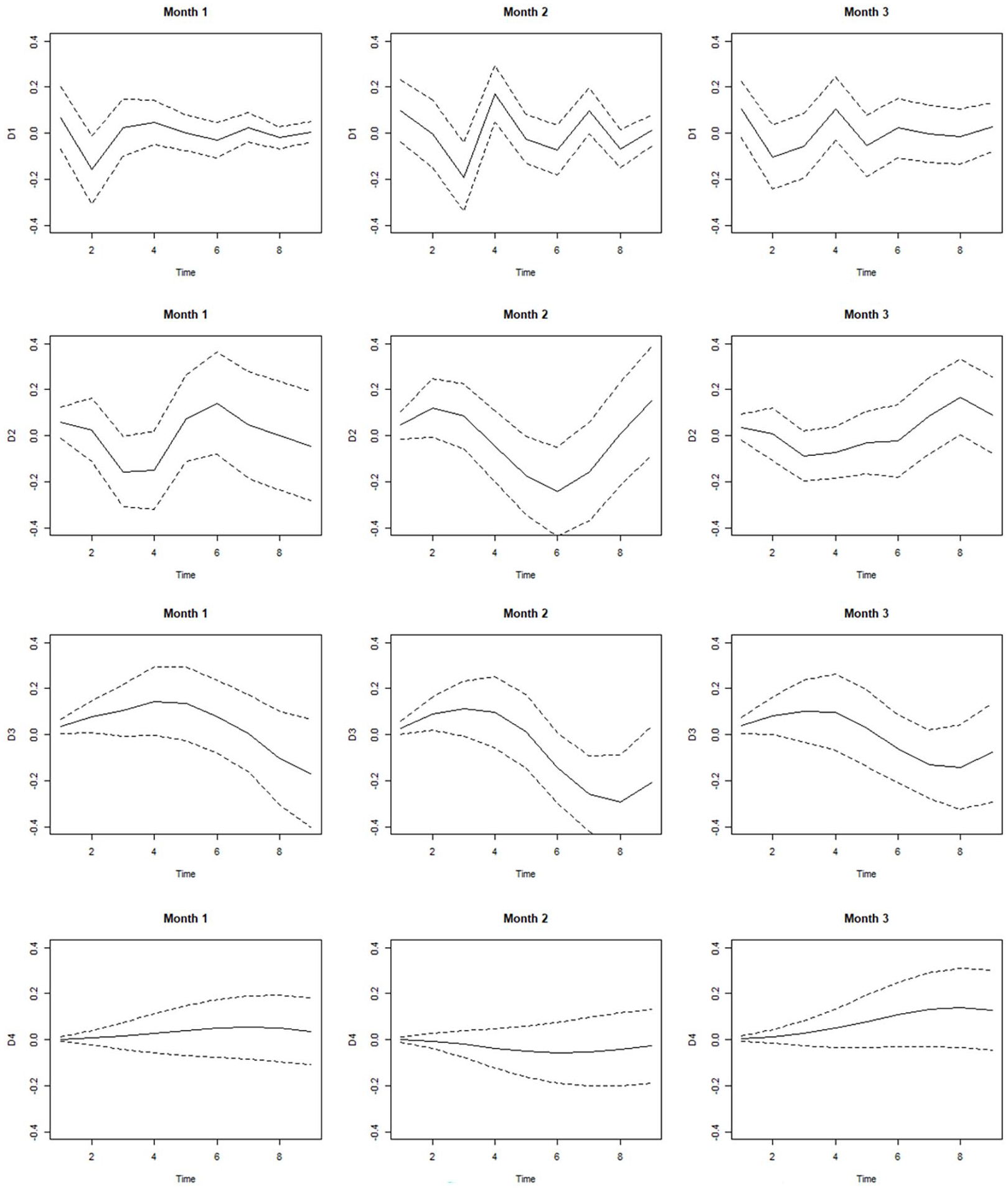
As noted in the literature and theory sections, the signs of the causal relationship between oil prices and economic activity are important to investigate and can vary for different country profiles and for different time horizons. Therefore, we continue to look at the impulse response functions. Months 1, 2, and 3 denote the three consecutive months that are included in the MIDAS framework because real GDP is quarterly data, while real oil prices are used on a monthly basis. D1, D2, D3, and D4 on the vertical axis represent the wavelet scales. That is, D1 is associated with one to two quarters, D2 with two to four quarters, D3 with four to eight quarters, and D4 with four to eight quarters. Interpretations of the impulse response functions are considered together with the Granger causality test results. This means that the focus of the impulse response function analysis is on the wavelet scales at which statistically significant causal relationships, in the Granger sense, are identified.
Starting with China, the results of the Granger causality test in Table 6 show that there is no causal relationship between real oil prices and real GDP at the D1 wavelet scale. Hence, we focus on the wavelet scales D2 (two to four quarters), D3 (four to eight quarters), and D4 (eight to sixteen quarters) and the associated impulse response function of China in Figure 5. We notice significant positive impulse responses of real GDP in China at those wavelet scales (D2, D3, and D4) to a rise in the oil price, although there are some insignificant responses. This result does not seem to align with the conventional understanding that an increase in oil price hampers economic activity for an oil importer. However, some explanations—albeit partial—for this finding for China may be as follows. First, a rise in oil prices may reflect the burgeoning global demand for oil and economic upturns from the major trading partners of China. As the evidence from Du, He and Wei (2010) shows that both oil prices and Chinese economic activity are dependent on the economic activity of the U.S. and European Union, the positive response of Chinese real GDP to an increase in oil prices can be explained by Chinese exports increasing with economic upturns among these trading partners. This explanation, therefore, aligns with the fact that an oil demand shock caused by global economic activity has a common positive effect on GDP across developing economies, as discussed in Section 2. This positive effect of oil price shocks on Chinese output has been reported in several previous studies (Du, He and Wei 2010; Wei and Guo 2016).
Impulse responses of the real GDP of China to an oil price shock.
Together with the results from Herwarts and Plödt (2016), our results reconcile the fact that oil price shocks positively affected the Chinese economy during this sample period with the aggregate global demand shock that has been dominant over other types of shocks. Second, as briefly noted in the introduction section, China’s country profile is dissimilar to that of the other economies in the sense that it is the world’s largest importer of oil; however, it has domestic production capacity (seventh place worldwide for production, according to the BP Statistical Review of World Energy, 2020), and it is the second largest refiner of oil. Although China is an importer of oil, its domestic oil production and sales of refined oil to other nations more than compensate for the negative effects of the oil price on production costs and economic activity.
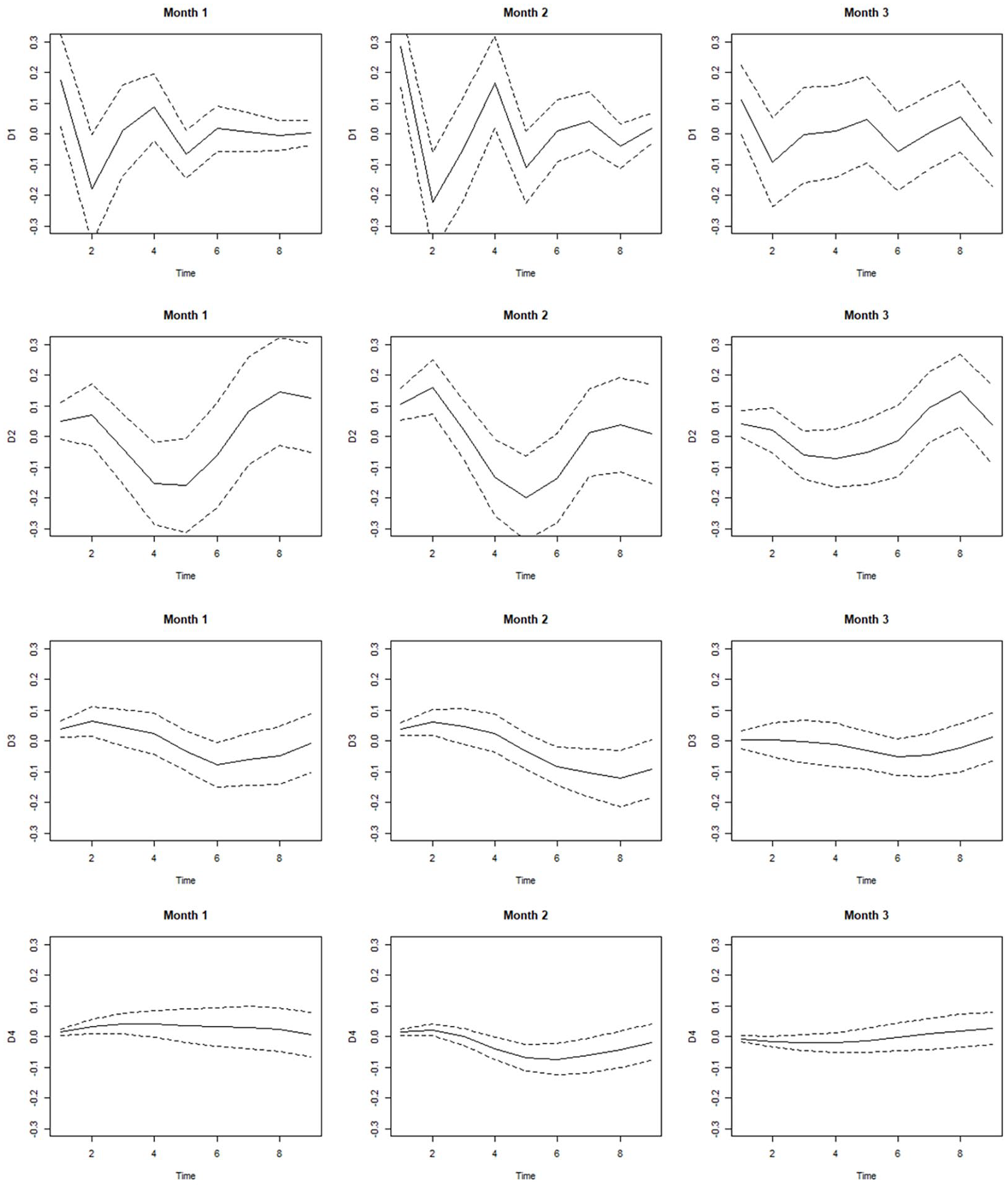
Regarding the responses of Japanese economic activity shown in Figure 6, attention is given to D1, D2, and D3 along with the Granger causality test results in Table 6. For wavelet scales D1 (one to two quarters) and D2 (two to four quarters), significant and positive Japanese real GDP responses to a rise in oil prices are detected. However, for wavelet scale D3 (four to eight quarters), significant negative reactions of economic activity start to appear. Our findings regarding the oil-GDP nexus in Japan share both similarities and contrasts with those of earlier studies. Zhang (2008) reports that GDP growth responds to oil price fluctuations most clearly in the first and fourth quarters, indicating both immediate and lagged effects. The authors also noted the nonlinear asymmetric effects of oil prices on production. Our findings add to the previous findings by providing further clarifications; we demonstrate that the responses in production change signs in response to oil price fluctuations in Japan across different time scales, ranging from a quarter to two years.
Impulse responses of the real GDP of Japan to an oil price shock.
This pattern of switching from positive to negative signs in the causal relationship from oil price to GDP is also illustrated in Figure 7 for Singapore. Differently, the negative signs start to appear from the D2 wavelet scale for Singapore, and the magnitude of the responses for Singapore is smaller than that for Japan. These two economies share the same major trading partners (including the U.S., European Union, and ASEAN economies); however, the category composition of the different exports may be behind these different magnitudes of the impact of oil prices on real GDP. 19 By comparing these countries’ economic output structures for exports, we can see that Japan relies somewhat more than Singapore on transport equipment, motor vehicles and machinery, which can be negatively influenced by an increase in oil prices. Although the issue of a change in sign was not discussed in Chang and Wong (2003), they also documented an insignificant oil price effect on GDP by suggesting evidence of a declining trend in oil intensity in Singapore.
Impulse responses of the real GDP of Singapore to an oil price shock.
Regarding the impulse response functions of Thailand in Figure 8, all wavelet scales are considered for interpretation since the Granger causality results are significant for all wavelet scales in Table 6. The responses of Thai domestic production show both similarities and dissimilarities with those of the other three aforementioned economies thus far, namely, China, Japan, and Singapore. The commonalities for all these economies are that the economic activity of all three aforementioned economies responds positively to a rise in oil prices at wavelet scales of at least one to two quarters (D1) and two to four quarters (D2), consistent with demand-driven effects of oil on output for these economies. However, unlike China, Thailand, which is also a developing economy, does not show significant positive causal relationships between real oil prices and real GDP across all time scales; rather, it does so only at the shortest time scale of one to two quarters. Additionally, concerning the negative responses of production in Thailand to oil price increases for wavelet scale D3 (four to eight quarters), they exhibit a lesser magnitude than do the other economies. Our findings for Thailand align with those of a previous study, Basnet and Upadhyaya (2015), which documented the role of oil subsidization in the economy, mitigating the impact of oil prices on economic performance. These varied production responses to oil prices in the two developing economies (China and Thailand) underscore their distinct characteristics, even when they are compared at a comparable level of economic development.
Impulse responses of the real GDP of Thailand to an oil price shock.
One economy that also demonstrates its own economic features is South Korea, whose impulse response functions are presented in Figure 9. Following the Granger causality results in Table 6, the interpretation of the impulse response functions for South Korea applies only for D3 and D4. On the time scales D3 (four to eight quarters) and D4 (eight to sixteen quarters), a significant and positive causal relationship from the oil price to economic activity is not clearly observed in Figure 9. This finding is consistent with those of several previous empirical studies on South Korea (Khan, Husnain and Abbas 2019). However, the results of the current study show a somewhat negative effect on Korean real GDP from an oil price shock at the scale of four to eight quarters (D3). As presented previously, the economic activity of the other four economies (China, Japan, Singapore, and Thailand) showed positive responses (mostly at shorter time horizons) to an increase in oil prices. This is due to the allegedly dominant demand-driven effects of oil on output for those economies. However, the South Korean economy does not follow this trend, suggesting that South Korean economic activity is not boosted as much as other Asian economies are during a buoyant period in the world economy. Somewhat negative responses to economic activity are observed at longer time horizons, yet they are not very conspicuous at time scales of up to four years, implying that the feasible negative impact of an oil price increase is well cushioned into the Korean economy through the economic policy channels of monetary policy, at least to some extent. In addition, this might be partly explained by the country’s long-term energy policy plans, as noted by Cunado, Jo and de Gracia (2015).
Impulse responses of the real GDP of South Korea to an oil price shock.
Overall, by examining the results for impulse-response functions in Figures 5 to 9, we can see that positive signs tend to be dominant at the smaller wavelet scales of one to two quarters (D1) and two to four quarters (D2), although not all of them represent statistically significant impulse responses. The general pattern of positive responses in economic activity to an oil price increase at time scales of up to a year does not seem to align with theories about the oil–economy nexus for oil importers versus oil exporters given that all of these economies are oil importers. However, this can still be explained if we consider two mechanisms. The first mechanism regards the underlying reasons for oil price increases. These economies are world-leading exporters of goods and services; thus, an increase in oil prices caused by strong global demand might have resulted in a positive response in real GDP through an increase in exports from these economies to the world market. This result is in line with the findings of Khan, Husnain and Abbas (2019), who document that oil demand shocks have a significant positive impact on real GDP in some Asian economies, while oil supply shocks have a limited impact. The other channel concerns domestic policy measures followed by an oil price increase, for example, monetary policy actions that involve a mechanism of transmission to economic activity. Accommodating the monetary policy of the authorities in these economies to counteract the increase in oil prices, which influences exchange rates, could also cause a positive response in economic activity.
At the larger wavelet scales of four to eight quarters (D3) and eight to sixteen quarters (D4), the abovementioned positive reaction of economic activity to oil price increases, in general, into a negative one. This suggests that the cost adjustment explanation (Hamilton 1988) applies at a time scale longer than two years. This finding is also consistent with price stickiness (along with energy contracts that pin down energy prices for a time span) in the shorter time span, although prices become less sticky in the longer time span. The unnoticeable negative effects of an oil price increase, even over time scales of up to four years, as found for South Korea, might suggest that the country has long-term energy policy plans. At least partly, this might have contributed to weakening the influence of oil as an important source of energy for production. A clear exception, to the abovementioned general pattern is China, which has a distinct character in terms of its domestic oil production and refinery capacity.
Our findings, based on the time-varying relationship, have important implications for the analysis of oil production and policy decision-making. First, it is very important to use disaggregated data that show the relationships between these two important macroeconomic variables, which are otherwise masked in the analysis using aggregate data. Second, it is essential to recognize that the effects of oil prices on production differ across various time scales. While an oil price increase is typically viewed as negative news for these Asian economies, the adverse effects on production manifest with a lag and are generally preceded by positive responses. This dynamic mechanism between oil prices and production should thus be incorporated into the decision-making process for short-run stabilization policy. Moreover, investigating country-specific responses is crucial. Although the five Asian economies included in the study share relatively similar characteristics in terms of their economic development phases and degree of oil dependence for production activities, the impact of oil prices on production varies across countries. This divergence includes the lag length that passes before the positive responses of production turn negative following an increase in the price of oil, as well as the variations in magnitude. A relevant aspect in understanding country-specific responses pertains to the diverse energy policies of the economies, encompassing plans to balance energy supply and demand, and the provision of fossil fuel subsidies. In essence, policymakers must recognize that the dynamics of production responses and other pertinent factors may differ at different time horizons, encompassing variations in both magnitude and signs. The relationship between energy resources and economic performance is not very deterministic; rather, it is largely driven by a mixture of economic policies, which have temporal dynamics.
7. Conclusion
This paper investigates the causal relationship between oil prices and economic activity for five selected Asian economies. We acknowledge that the literature in this field has indicated the need to differentiate different types of oil shocks when analyzing the effects of oil price changes on macroeconomic indicators. Identification of the different oil shocks and varying effects, however, was not performed in the present study. We instead resort to the previous literature that identifies the different shocks that remain controversial (Herwartz and Plödt 2016), noting that the restrictions imposed to identify supply and demand shocks by Kilian (2009) are based on the assumption of a vertical short-run supply of crude oil. Thus, rather than identifying different types of oil shocks, we employ the MIDAS approach to fully exploit available information and disaggregate the data into different layers of time scales using the wavelet transform. Specifically, for the empirical analysis in the present paper, we employ the U-MIDAS for monthly real oil data and quarterly data for real GDP. The causal relationship between real oil prices and real GDP is also studied with wavelet-transformed data to investigate whether the relationship between the variables changes over different time scales.
The key empirical results of the present paper show that there is a clear significant causal link from oil prices to economic activity under the MIDAS approach, which is not as clearly found using the standard VAR approach. To investigate the signs of the relationship between real oil prices and economic activity, impulse response functions are analyzed along with the significance of the Granger causality results. Our results suggest that the five Asian economies, in general, respond positively to an increase in oil prices at shorter time horizons (less than two years), while the positive responses change mostly in a negative direction at longer time horizons (two to four years). Therefore, we provide evidence for the (theoretically) expected negative nexus between real oil prices and economic activity for oil importers over longer time horizons for our dataset. An exception to this pattern is China, which shows a positive response in domestic production to an increase in oil prices across all time scales. This may be explained by the country’s economic output structure, which includes domestic oil production and increasing refinery capacity. Another distinctive feature is also found for the South Korean economy, which does not show a positive response in production to an oil price increase, while all the other economies respond positively. Its economy shows a somewhat negative response in production at the time scale of two to four years, yet this response is not clearly noticeable. Insights from these findings can be drawn from the perspective of broader policy, including long-term energy policy and monetary policy, which accommodates oil price shocks in the economy.
Employing a MIDAS model in the wavelet context is a novel approach to investigating the causal relationship between oil prices and economic activity. The MIDAS model enables us to utilize the data without losing information while matching the frequencies of observation, as our results show. In addition, using wavelet-transformed data avoids the problem of nonstationarity and mitigates the problem of structural breaks to some degree. In sum, our findings suggest that the conventional wisdom about the effects of oil prices on macroeconomic activity can be misleading if the economic output structure and monetary and exchange rate mechanisms that cushion the effects are disregarded. The effects also manifest at different time scales in combination with the mechanisms used for the policy measures. Notably, when we discuss time scale–varying causal relationships between oil price movements and economic activity, we use wavelet scales (e.g., two to four quarters and eight to sixteen quarters) instead of the typical, yet ambiguous, categorizations of time horizons as short and long term. The mixed findings of previous studies may be due to the use of such coarse time horizons. More precisely, there are rules of thumb in economics that put horizons of two to three years in the realm of the short run due to some contracts (such as wage contracts) that resist price changes. However, two to three years are longer time horizons than a year or less. The short and long runs of the usual time-series methods using VECM and cointegration approaches have an even coarser categorization of time horizons. Some inconsistent findings of empirical studies in the literature, therefore, could have resulted from using such unclear time-horizon classifications using data at different frequencies. In addition, the problem of aligning macroeconomic indicators at varying frequencies of observation to a common low frequency may also cause the loss of important information when investigating the relationships of the variables. The findings of this study using MIDAS with wavelet analysis, therefore, add to the literature since we utilized the data without losing information when matching the frequencies of observation. In addition, this study disentangles the specific relationships between oil price fluctuations and economic activity at different time scales.
Description
The key empirical results under unrestricted MIDAS (U-MIDAS) approach show that there is a clear significant causal link from oil prices to economic activity, which is not as clearly found under the standard VAR approach. In addition, the results of the paper using impulse response functions suggest that the five Asian economies respond, in general, positively in economic activity to an oil price shock at shorter time horizons (less than two years), while the positive responses switch to mostly negative ones at longer time horizons (from two to four years). An exception to this pattern is China, which has a dissimilar country profile.
Footnotes
Declaration of Conflicting Interests
The author(s) declared no potential conflicts of interest with respect to the research, authorship, and/or publication of this article.
Funding
The author(s) received no financial support for the research, authorship, and/or publication of this article.
1
For example, see the Wall Street Journal, “The oil slump threatens Norway’s economy,” December 4, 2014 at http://www.wsj.com/articles/oils-slump-threatens-norways-economy-1417721313; “Russia says economy could recover soon thanks to rising oil prices,” October 25, 2016 at http://www.wsj.com/articles/russia-says-economy-could-recover-soon-thanks-to-rising-oil-prices-1460477143; “Canadian dollar recovers on higher oil prices and hopes for economy,” March 3, 2016 at http://www.wsj.com/articles/canadian-dollar-recovers-on-higher-oil-prices-and-hopes-for-economy-1457041897; “Markets rise after lockdowns prompt oil price plunge,” November 2, 2020 at https://www.bbc.com/news/business-54775143; and “Fiscal stimulus, vaccine rollouts brightens OPEC’s oil demand forecast,” March 11, 2021 at ![]() .
.
2
3
4
The countries that were initially considered for inclusion in the study but eventually excluded are India, Malaysia, and Indonesia. This exclusion is primarily attributable to data issues. Specifically, India has three-month or ninety-day rates and yield data available only from 2010, while Malaysia has real GDP data only from 2010 and Indonesia has data available from 2000. This data is sourced from the FRED database, which is used for collecting the data in the study.
5
Along with other OECD economies from 1973 to 1982. Unlike other OECD economies, which showed a minimal impact of oil-price innovations on the price level and production for the 1979 to 1980 shocks, the oil price increased Japanese inflation and slowed output growth.
7
The least asymmetric (LA) wavelet filter is a common choice in empirical studies (see, e.g., Ramsey and Lampart (1998), ![]() due to its ability to provide the most accurate time-alignment between wavelet coefficients at various scales and the original time series.
due to its ability to provide the most accurate time-alignment between wavelet coefficients at various scales and the original time series.
9
Further explanations on the robustness check are followed in Footnote 18.
10
The sample period starts from 1998Q1 and avoids the structural breaks in the variables of interest, which affected many economies in the region in 1997. For example, South Korea transitioned to free-floating exchange rate regime from the market average rate system in December 1997, while Thailand shifted to a managed floating system from the fixed exchange rate in July 1997. In the same context, the sample period does not include the most recent years, marked by intensive fluctuations in oil prices due to the COVID-19 pandemic and the war in Ukraine.
12
The price index used is the Consumer Price Index: All Items for the United States, Index 2015=100, Monthly, Not Seasonally Adjusted.
13
14
The REER is the weighted average of a country’s currency relative to an index or basket of other major currencies and adjust for the effects of inflation.
15
To save space, we do not include the wavelet details of real GDP for other economies in the study. They are, however, available from the authors upon request.
16
The other direction of causality, from real GDP to real oil prices is additionally investigated, and the results are available upon request.
17
It is, however, worthwhile to note that China is included in this study, and the investigation results on the effect of oil shocks on its economic activity do reveal distinctive features of the economy.
18
Explanations in detail on the robustness check are the followings. We use two approaches to handle the issue of parameter proliferation when more independent variables are included. The first method is taken from Hacker et al. (2012). Instead of using the original variables in equation (4), we use the residuals from an OLS model where GDP and oil prices are regressed on inflation rates, exchange rates and interest rates. The second approach is taken from ![]() , where only one lag of all variables is used in the VAR model; subsequently, to account for potential autocorrelation, Newey and West’s heteroscedasticity and autocorrelation consistent covariance matrix are used when testing for Granger causality. For the impulse response function, we use only the orthogonalized data to avoid autocorrelation in the error term.
, where only one lag of all variables is used in the VAR model; subsequently, to account for potential autocorrelation, Newey and West’s heteroscedasticity and autocorrelation consistent covariance matrix are used when testing for Granger causality. For the impulse response function, we use only the orthogonalized data to avoid autocorrelation in the error term.
19
According to the World Integrated Trade Solutions (WITS) of the World Bank, the top five exported HS 6-digit-level products are monolithic integrated circuits, petroleum oils (excl. crude), gold in other semi-manufactured forms, transmissions apparatuses, and parts and accessories for automatic data processing. The top five exports for Japan are occupied by automobile parts, monolithic integrated circuits and motor vehicles.