Design Parameters for Planning the Sample Size of Individual-Level Randomized Controlled Trials in Community Colleges

Abstract

The last two decades have seen a dramatic increase in randomized controlled trials (RCTs) conducted in community colleges. Yet, there is limited empirical information on the design parameters necessary to plan the sample size for RCTs in this context. For a blocked student-level random assignment research design, key design parameters for the minimum detectable true effect (MDTE) are the within-block outcome standard deviation $\left({\sigma }_{|\mathit{S}}\right)$ and the within-block outcome variance explained by baseline covariates like student characteristics $\left(R_{|\mathit{S}}^2\right)$ . We provide empirical estimates of these key design parameters, discussing the pattern of estimates across outcomes (enrollment, credits earned, credential attainment, and grade point average), semesters, and studies. The main analyses use student-level data from 8 to 14 RCTs including 5,649–7,099 students (depending on the outcome) with follow-up data for 3 years. The following patterns are observed: the within-block standard deviation $\left({\sigma }_{|\mathit{S}}\right)$ and therefore the MDTE can be much larger in later semesters for enrollment outcomes and cumulative credits earned; there is substantial variation across studies in ${\sigma }_{|\mathit{S}}$ for degree attainment; and baseline covariates explain less than 10% of the variation in student outcomes. These findings indicate that when planning the sample size for a study, researchers should be mindful of the follow-up period, use a range of values to calculate the MDTE for outcomes that vary across studies, and assume a value of $R_{|\mathit{S}}^2$ between 0 and 0.05. A public database created for this paper includes parameter estimates for additional RCTs and students.

Introduction

Community colleges (CCs) play a vital role in U.S. postsecondary education. In Fall 2017, CCs served nearly six million students, representing 39% of all U.S. undergraduates (Ginder et al., 2018, Table 3). Despite providing unprecedented access to postsecondary education, rates of degree attainment remain low. Among first-time, full-time, degree/certificate-seeking students whose first postsecondary school is a 2-year public institution, only 25% graduate within 3 years (McFarland et al., 2019, p. 199). To address these issues, policymakers, foundations, and college administrators are beginning to embrace the need for causal evidence of the effectiveness of postsecondary programs, policies, and practices.

In 2002, the U.S. Department of Education created the Institute for Educational Sciences (IES) as part of the Education Sciences Reform Act. IES has provided unprecedented funding for educational evaluations with strong potential to draw causal conclusions. This advance nearly coincided with MDRC launching the first ever large scale (n = 1500) randomized controlled trial (RCT) at a CC (Bloom & Sommo, 2005).

Thus began a transformation in higher education evaluation. Two decades later, MDRC alone has conducted RCTs of just over 30 interventions in over 45 (mostly community) colleges throughout the United States, including 67,400 students, mostly from low-income families (Diamond et al., 2021). Many more RCTs in higher education have been conducted by others. For example, the What Works Clearinghouse (WWC) has published reviews of 48 postsecondary RCTs that meet their evidence standards without reservations. ¹

While the number of RCTs in CCs has grown dramatically over the past 20 years, the information needed to plan a high-quality RCT in this context has not. Several types of information are important for designing an RCT that will produce impact findings that are reliably estimated. Among other things, it is important to have information about the design parameters that affect the sample size necessary so that the study can be powered to confidently detect effects of a pre-specified size. Unfortunately, this information is scarce in the CC context.

In this article, we provide empirical estimates of the design parameters needed to conduct individual-level RCTs in CCs. To do so, we rely on student-level data from the RCTs that MDRC has conducted since 2001. Design parameters are estimated for each RCT at six timepoints (ranging from one semester to 3 years after random assignment) for four outcomes that are commonly considered confirmatory in community college RCTs—enrollment/persistence, credits earned, GPA, and degree completion. The goal is that this information will serve as a resource to researchers looking to conduct well-powered RCTs in the postsecondary education context.

Some Relevant Context

In the last decade and a half, great strides have been made to generate methodological tools and benchmarks to support the design and planning of RCT evaluations in K-12 education. K-12 researchers now have available estimates of the design parameters necessary for conducting statistical power analyses (e.g., see: Bloom, Zhu et al., 2008; Deke et al., 2010; Dong et al., 2016, 2021; Hedberg, 2016; Hedges & Hedberg, 2007a, 2007b, 2014; Jacob et al., 2010; Kelcey et al., 2016; Jaciw et al., 2016; Juras, 2016; Schochet, 2008; Weiss et al., 2017; Westine et al., 2013; Xu & Nichols, 2010).

The result of these methodological advances in K-12 has been a major improvement in the information available to enable K-12 researchers to design RCTs that are well-powered and cost-efficient.

Unfortunately, design parameters for K-12 and postsecondary education are not interchangeable for several reasons. First, estimates of K-12 design parameters are largely based on cluster randomized trials (CRT), a design that is common in K-12 but rare in CC RCTs. In CCs, student-level randomization is the norm and the relevant design parameters are different. Second, existing design parameters in K-12 focus on the outcomes typically targeted by K-12 interventions—test scores, attendance, and socio-emotional outcomes. In contrast, CC RCTs typically focus on different outcomes—enrollment/persistence, credit accumulation, GPA, and credential attainment. Finally, and perhaps most importantly, design parameters estimated based on data from K-12 may not apply to CC studies due to differences in context, student characteristics, and available data. CC researchers are thus left without clear guidance when planning RCTs.

This may explain why many postsecondary RCTs appear to be underpowered. Consider the RCTs of the 48 postsecondary interventions listed as having met IES’s What Works Clearinghouse (WWC) standards without reservations—presumably, these are some of the highest quality postsecondary evaluations conducted to date. 12 out of 48 (25%) had a total sample size of under 350 students. If we consider reported subgroup analyses, 21 out of 48 (44%) conducted analyses on a sample of size 350 students or less. Under reasonable assumptions, the minimum detectable effect for a binary outcome (e.g., enrollment or degree completion) in a study with 350 sample members is 10–15 percentage points, ² which is quite large. ³ Reviews have found that many education studies (and not just CC RCTs) are not adequately powered (Cheung & Slavin, 2016; Spybrook et al., 2016; Torgerson et al., 2005).

There are many possible explanations for these low-powered studies. Researchers may not be conducting power analyses; they may be conducting power analyses but plugging in overly optimistic design parameters; they may have unrealistic expectations around what size intervention effects can reasonably be expected; or they might represent pilot studies that were not designed to detect intervention impacts at all or with great precision. Perhaps the most common reason is a matter of resource constraints, including time, money, and partnerships.

Whatever the reasons, there is much room for improvement, information, and education. Our aim with this paper is to eliminate the second of these reasons (plugging in overly optimistic design parameters), ensuring that postsecondary researchers have empirically derived information at their disposal for power calculations.

Design Parameters for Community Colleges Randomized Controlled Trials

Multiple design parameters influence the sample size required for an RCT. The relevant design parameters depend on the study design (e.g., cluster randomization vs. individual randomization) and the effect estimator. ⁴ In CC research, a design commonly used in RCTs to date involves randomizing individuals (college students) to experimental conditions, often within sites (sometimes called an “individually-randomized blocked” design). ⁵

Given this research design, the fixed-effects estimator is commonly selected to estimate the average treatment effect (Miratrix et al., 2021). For binary outcomes, many RCTs in higher education use linear probability models (LPM) to estimate program effects. ⁶ Logistic regression is also used. In this paper, we focus on LPMs given convincing arguments in favor of LPMs in the context of RCTs (Deke, 2014; Schochet, 2015).

When using a LPM, the fixed-effects estimator of the average effect of being offered the treatment ( $\delta$ ) at a total of $J$ sites (i.e., blocks) can be written as ⁷

$Y_i=\mathit{\alpha }\cdot {\mathit{S}}_{\mathit{i}}+\delta T_i+\mathit{\gamma }\cdot {\mathit{X}}_{\mathit{i}}+e_i,$

(1)

where ${\hspace{0.17em}Y}_i=$ the outcome for student $i$ ,

${\mathit{S}}_{\mathit{i}}=$ a vector of $J$ elements (one for each site, i.e., block, in the study) where the j^th element is equal to one if student $i$ was randomly assigned at site $j$ (typically colleges in this context) and zero otherwise,

$T_i=$ one if student $i$ was assigned to treatment and zero otherwise,

${\mathit{X}}_{\mathit{i}}=$ is a vector of $H$ elements (one for each baseline covariate) where the $h^{th}$ element equals the baseline covariate for student $i,$

$e_i=$ a random error that is independent and identically distributed across individuals.

We define the total unconditional variance of the outcome across all students as ${\sigma }^2$ . In equation (1), $VAR\left(e_i\right)\equiv {\sigma }_{|\mathit{X},\mathit{S}}^2$ , which is the residual variance of individual outcomes under the null hypothesis of no impact. The “ $|\mathit{X},\mathit{S}$ ” in ${\sigma }_{|\mathit{X},\mathit{S}}^2$ is used to specify that the residual variance is conditional on the site indicators ( $\mathit{S}$ ) and individual-level covariates ( $\mathit{X}$ ). ⁸

The statistical precision of this impact estimator can be described by its standard error as follows (adapted from: Bloom & Spybrook, 2017; Weiss et al., 2017)

$SE\left(\delta \right)=\sqrt{\frac{{\sigma }_{|\mathit{S}}^2\left(1-R_{|\mathit{S}}^2\right)}{J\overline{n}\overline{T}\left(1-\overline{T}\right)}},$

(2)

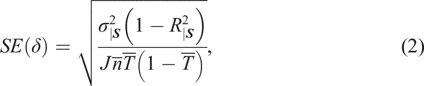
where ${\sigma }_{|\mathit{S}}^2$ is the within-site variance of the outcome, $R_{|\mathit{S}}^2$ is the proportion of ${\sigma }_{|\mathit{S}}^2$ that is predicted by the baseline covariates ( $\mathit{X}$ ) ⁹ , $J$ is the total number of sites, $\overline{n}$ is the mean number of sample members per site, and $\overline{T}$ is the proportion of sample members randomly assigned to the treatment group. ¹⁰ Notably, ${\sigma }_{|\mathit{X},\mathit{S}}^2={\sigma }_{|\mathit{S}}^2\left(1-R_{|\mathit{S}}^2\right)$ . That is, the numerator within equation (2) is the residual variance ( ${\sigma }_{|\mathit{X},\mathit{S}}^2$ ), which is the within-site outcome variance that is not explained by baseline covariates. ¹¹

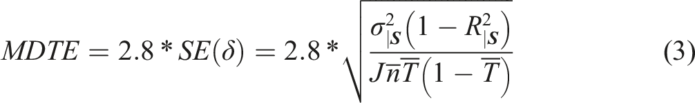
The Minimum Detectable True ¹² Effect, or MDTE, is the smallest true effect for which a study would have a $1-\beta$ percent chance of detecting the existence of an effect based on a two-tailed test of statistical significance at the $\alpha$ significance level. The MDTE is equal to $SE\left(\delta \right)$ (Equation (2)) times a multiplier whose value depends on the desired power ( $1-\beta$ ) and significance level ( $\alpha$ ). Common choices for power and significance are $1-\beta$ = 80% and α = 5%, which yields a multiplier of 2.8 when the sample size is reasonably large. ¹³ Thus, the MDTE can be written as (adapted from: Schochet, 2008; Bloom, 2008)

$MDTE=2.8*SE\left(\delta \right)=2.8*\sqrt{\frac{{\sigma }_{|\mathit{S}}^2\left(1-R_{|\mathit{S}}^2\right)}{J\overline{n}\overline{T}\left(1-\overline{T}\right)}}$

(3)

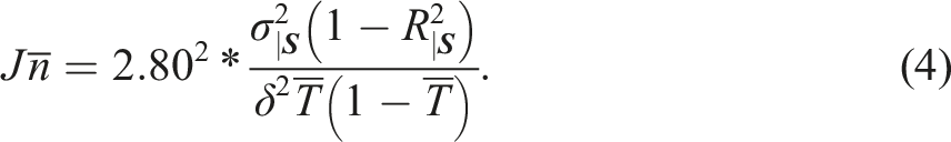
By re-arranging the terms in equation (3), we can calculate the total sample size ( $J\overline{n}$ ) required to achieve 80% power to detect a true effect of size $\delta$ at a 5% significance level

$J\overline{n}={2.80}^2*\frac{{\sigma }_{|\mathit{S}}^2\left(1-R_{|\mathit{S}}^2\right)}{{\delta }^2\overline{T}\left(1-\overline{T}\right)}.$

(4)

Equation (4) indicates how four factors influence the sample size necessary in an RCT. All else equal, the sample size required to achieve 80% power at the 5% significance level decreases as:

(1) the within-site outcome variance ( ${\sigma }_{|S}^2$ ) decreases,

(2) the proportion of the within-site outcome variance explained by covariates ( $R_{|\mathit{S}}^2$ ) increases,

(3) the true effect size ( $\delta$ ) increases, and

(4) the proportion of sample members assigned to treatment ( $\overline{T}$ ) is closer to 0.50. ¹⁴

As noted by Bloom (2005), $J$ , $\overline{n}$ , and $\overline{T}$ are “research design choices” and can often be modified (within reason) to ensure adequate statistical precision (e.g., by recruiting more sites to join an RCT). In contrast, ${\sigma }_{|\mathit{S}}^2$ “reflects the underlying variation in the outcome of interest, which must be taken as given” (Bloom, 2005, p. 128). $R_{|\mathit{S}}^2$ lies somewhere in between since collecting additional baseline data may yield an increased $R_{|\mathit{S}}^2$ , but the underlying covariate-outcome relationships that exist must also be taken as given. Thus, when planning an evaluation it is common to assume values for ${\sigma }_{|\mathit{S}}^2$ and $R_{|\mathit{S}}^2$ and then determine the number of sites, number of students per site, and the random assignment ratio necessary to detect meaningful (or realistic) program effects.

The present paper provides a series of estimates of ${\sigma }_{|S}$ (the within-block standard deviation) and $R_{|\mathit{S}}^2$ , providing an empirical foundation about these design parameters in CC studies for highly relevant outcomes, time points, and populations. Student-level data from RCTs conducted by MDRC are used to explore the following questions:

• What is the distribution of ${\sigma }_{|\mathrm{S}}$ and $R_{|\mathit{S}}^2$ estimates in student-level RCTs of CC interventions, by outcome and by follow-up semester?

• Are there notable patterns of variation in these parameters across semesters? Across studies?

• Can $R_{|\mathit{S}}^2$ be appreciably improved with a richer set of baseline covariates?

In the next section of this paper, we describe the data sources and outcome measures used in our analyses as well as our approach to estimating these design parameters. In the following section, we share results. Finally, in the last section, we offer a discussion of recommendations and areas for future research.

Methods

Studies and Analysis Sample, Data Sources, and Measures

Studies and Analysis Sample

The present analyses are based on 16 RCTs that MDRC has conducted in postsecondary education. These RCTs were selected because they collected data on student outcomes for the first six semesters after random assignment (a common time period to consider community college degree completion rates), thereby making it possible to examine the pattern of variation in the design parameters across semesters of follow-up as well as across studies.

For each of these studies, the main analytic sample includes control group students in the study cohorts that were followed for 6 semesters. Restricting the sample to control students ensures that the design parameters are estimated under the null hypothesis of no effects. The number of control students in each study is sufficiently large to estimate the design parameters such that any precision loss does not pose a problem. ¹⁵ Restricting the analytic sample to cohorts with six semesters of follow-up ensures that, for a given outcome, any time trend in the estimated distribution of a design parameter is more likely attributable to real changes over time, rather than changes in the studies or students included in the analyses.

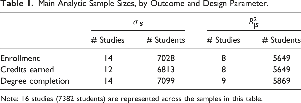
Because data availability varies across studies, the main analytic sample is defined separately for each outcome and by design parameter in order to maximize the available sample for each analysis. (For analyses of $R_{|\mathit{S}}^2$ we include one additional restriction at the study level—the ratio of observations to potential baseline covariates must be at least 10:1 to avoid an over-specified regression model.) Table 1 shows the number of studies and students used to estimate the design parameters for each outcome, ranging from 8 to 14 studies and 5649 to 7099 students. A total of 16 studies conducted in nine states are represented in these samples.

Table 1.

Main Analytic Sample Sizes, by Outcome and Design Parameter.

	${\sigma }_{|\mathit{S}}$		$R_{|\mathit{S}}^2$
	# Studies	# Students	# Studies	# Students
Enrollment	14	7028	8	5649
Credits earned	12	6813	8	5649
Degree completion	14	7099	9	5869

Note: 16 studies (7382 students) are represented across the samples in this table.

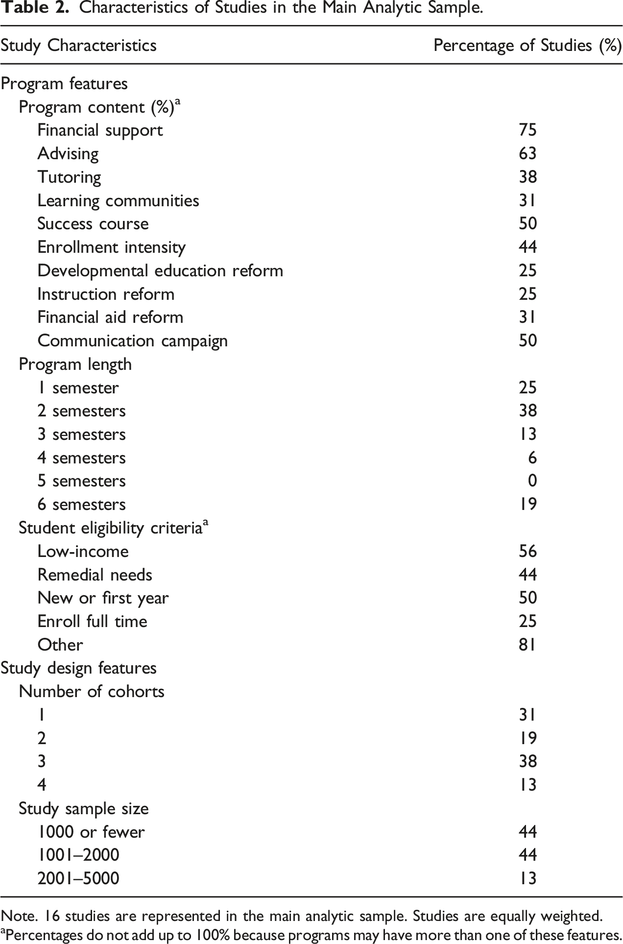
As shown in Table 2, these 16 studies evaluated the effect of interventions that vary in their duration (from one semester to 3 years) and key components (e.g., advising, tutoring, and financial supports). The target population for all studies is students enrolled in the colleges (as opposed to prospective students or applicants); in half of the studies, eligibility was limited to new or first year students. Most were conducted at CCs or public universities with large populations of students from families with low-income (or the studies targeted students from families with low-income) and most studies include multiple cohorts.

Table 2.

Characteristics of Studies in the Main Analytic Sample.

Study Characteristics	Percentage of Studies (%)
Program features
Program content (%) a
Financial support	75
Advising	63
Tutoring	38
Learning communities	31
Success course	50
Enrollment intensity	44
Developmental education reform	25
Instruction reform	25
Financial aid reform	31
Communication campaign	50
Program length
1 semester	25
2 semesters	38
3 semesters	13
4 semesters	6
5 semesters	0
6 semesters	19
Student eligibility criteria a
Low-income	56
Remedial needs	44
New or first year	50
Enroll full time	25
Other	81
Study design features
Number of cohorts
1	31
2	19
3	38
4	13
Study sample size
1000 or fewer	44
1001–2000	44
2001–5000	13

Note. 16 studies are represented in the main analytic sample. Studies are equally weighted.

^aPercentages do not add up to 100% because programs may have more than one of these features.

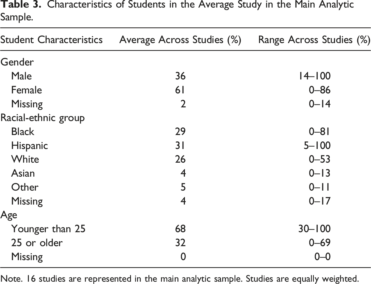
Reflecting national patterns in 2-year colleges, in the average study 62% of students are female and the majority of students (71%) are younger than 25 (see Table 3). About two thirds of students in the average study are Black or Hispanic, more than in the average 2-year college in the US. However, there is substantial variation in the characteristics of students across the studies; for example, the percentage of female students ranges from 0 to 86%, and the percentage of white students ranges from 0 to 53%.

Table 3.

Characteristics of Students in the Average Study in the Main Analytic Sample.

Student Characteristics	Average Across Studies (%)	Range Across Studies (%)
Gender
Male	36	14–100
Female	61	0–86
Missing	2	0–14
Racial-ethnic group
Black	29	0–81
Hispanic	31	5–100
White	26	0–53
Asian	4	0–13
Other	5	0–11
Missing	4	0–17
Age
Younger than 25	68	30–100
25 or older	32	0–69
Missing	0	0–0

Note. 16 studies are represented in the main analytic sample. Studies are equally weighted.

Because the data used for the present analysis are from actual RCTs, all of which focus on students who are already enrolled, the design parameters presented in this paper may not generalize to the outcome variation that one would observe for all community college students in the US, nor to prospective students or applicants to these colleges. However, the findings are likely to represent the range of parameter values that researchers will encounter for the subset of colleges and enrolled students that agree to participate in CC RCTs.

Data Sources and Measures

Data for the 16 studies included in the present analysis are from The Higher Education Randomized Controlled Trials (THE-RCT) student-level database. This database includes all the RCTs that MDRC has conducted in postsecondary education since 2003, representing RCTs of over 30 interventions conducted across more than 45 postsecondary institutions and 12 states with 67,400 students (Diamond et al., 2021). For details about the individual studies, see Diamond et al. (2021). For reasons noted earlier, this paper focuses on the subset of studies with at least six semesters of follow-up data. However, study-level estimates of the design parameters for the full set of studies and students in the THE-RCT database are available in a public-use dataset created for this paper and available from the authors on request. The values (and pattern) of design parameter estimates for the full sample are similar to those for the analytic samples.

In all studies, data on students’ outcomes and their baseline characteristics come from three sources: (1) college (or college system) records, which include demographic records, placement test data, course transcripts, grade point average (GPA), and degree completion; (2) data from the National Student Clearinghouse (NSC), which includes information on enrollment and degree completion from nearly 3600 colleges that combined enroll over 97% of the nation’s college students ¹⁶ ; and (3) a study-administered student survey implemented at the time of random assignment, which includes more detailed information on student characteristics that are not available from college records.

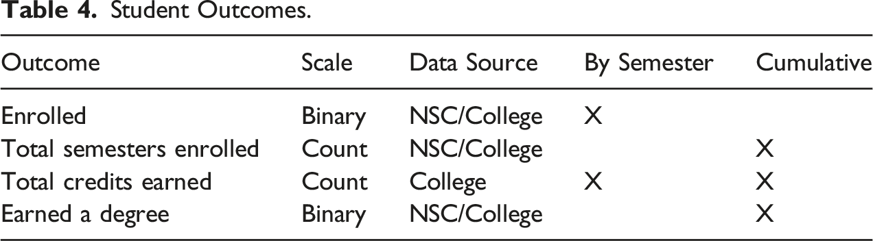
Student Outcomes

The outcomes explored in the present analysis, summarized in Table 4, are the focus of most CC interventions: enrollment (by follow-up semester and the cumulative number of semesters enrolled during a specified follow-up period), credits earned (by semester and cumulatively), and degree completion. Data on the number of credits earned were obtained from college records. Information on enrollment and degree completion are available from college data or from the NSC, depending on the study and the student. Therefore, to maximize data availability across studies, these outcomes are derived using both data sources. When only college/system outcome data are available for a student, these measures are defined as enrollment or degree completion at the college/system of random assignment. When both college/system and NSC data are available, these outcomes are defined as enrollment or degree completion at any college/university covered by the two sources. ¹⁷

Table 4.

Student Outcomes.

Outcome	Scale	Data Source	By Semester	Cumulative
Enrolled	Binary	NSC/College	X
Total semesters enrolled	Count	NSC/College		X
Total credits earned	Count	College	X	X
Earned a degree	Binary	NSC/College		X

Attrition of sample members does not present a problem in our analyses. For enrollment, credit accumulation, and degree completion, data are available for every student in the study, as long as the relevant information (e.g., transcript records for credit accumulation) was collected for that study. When the college or NSC data include no records for a given student, we treat that student as not being enrolled, and therefore earning zero credits and not earning a degree.

As a supplemental analysis, we also examine students’ performance in their courses as measured by their grade point average (GPA), measured on a 4-point scale. ¹⁸ Impacts on GPA are challenging to evaluate in postsecondary impact studies because GPA is only defined for students who are still enrolled. This means that if an intervention has an impact on enrollment, estimated effects on GPA could be biased (and in all cases, estimated effects on GPA do not apply to unenrolled students). For the present analysis, comparing the standard deviation of GPA across follow-up semesters is also challenging because attrition from the sample increases over time. Therefore, the findings for GPA in this paper are limited to the first follow-up semester and discussed separately.

Student Characteristics at Baseline

Information about students’ characteristics at baseline (and related baseline variables) come from college records and student baseline surveys:

• College records. College records typically include demographic characteristics like age, race and ethnicity, and gender; educational background factors like previous credentials; and financial aid information like Pell eligibility and Expected Family Contribution (EFC).

• Baseline surveys. The information collected from surveys varies across studies, but includes measures across domains such as: Financial aid (e.g., Pell status); measures of socioeconomic status (e.g., public assistance, parent education); diplomas/degrees previously earned (e.g., HS diploma/GED); family and household characteristics (e.g., age of youngest child, number of children, language spoken at home); earnings and employment; and access to transportation and educational tools (e.g., has vehicle to commute, home computer). For a more comprehensive list of available baseline characteristics, see the codebook in Diamond et al. (2021).

• Placement tests. Some studies collected data on students’ performance on placement tests, which are sometimes available from college records. A total of 29 different placement tests across 10 studies are represented. For the purposes of the analysis, students who took the same test more than once are assigned their best score in the 3 years prior to random assignment.

As discussed in the next section, empirical estimates of $R_{|\mathit{S}}^2$ are derived for various combinations of these baseline characteristics. Because the majority of students are new or first-year students, college outcomes from prior semesters (GPA, credits earned) are not examined as baseline covariates in this analysis.

Estimation of Design Parameters

As noted earlier, the goal of the present analysis is to produce estimates of two key design parameters—the within-block outcome standard deviation ( ${\sigma }_{|S}$ ) and the proportion of within-block outcome variation that is explained by the covariates ( $R_{|\mathit{S}}^2$ )—for each study in the analytic sample, by outcome and by semester of follow-up. Most studies in the dataset include multiple cohorts and more than one college, so blocks are typically defined as college-by-cohort.

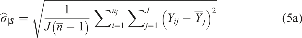
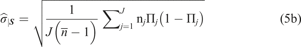
For each study, we estimate the within-block standard deviation of the outcome, ${\sigma }_{|\mathit{S}}$ , as follows

${\widehat{\sigma }}_{|\mathit{S}}=\sqrt{\frac{1}{J\left(\overline{n}-1\right)}{\displaystyle \sum }_{i=1}^{n_j}{\displaystyle \sum }_{j=1}^J{\left(Y_{ij}-{\overline{Y}}_j\right)}^2}$

(5a)

where J is the number of blocks, $\overline{n}$ is the average number of students per block, $Y_{ij}$ is the outcome for student i in block j, and ${\overline{Y}}_j$ is the mean outcome for students in block j. For a binary outcome, equation (5a) simplifies to (adapted from Bloom, 1995)

${\widehat{\sigma }}_{|\mathit{S}}=\sqrt{\frac{1}{J\left(\overline{n}-1\right)}{\displaystyle \sum }_{j=1}^J{\mathrm{n}}_j{\mathrm{\Pi }}_j\left(1-{\mathrm{\Pi }}_j\right)}$

(5b)

where $\mathrm{\Pi }$ is the proportion of the study population that would have a value of 1 for the binary outcome. ¹⁹ Separate estimates are obtained for each study by outcome measure and by follow-up semester, based on the relevant analytic sample.

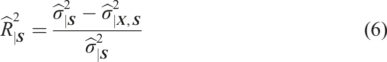
For each study, we estimate the proportion of within-block outcome variation explained by the baseline covariates, $R_{|\mathbf{S}}^2$ , as follows

${\widehat{R}}_{|\mathit{S}}^2=\frac{{\widehat{\sigma }}_{|\mathit{S}}^2-{\widehat{\sigma }}_{|\mathit{X},\mathit{S}}^2}{{\widehat{\sigma }}_{|\mathit{S}}^2}$

(6)

where ${\widehat{\sigma }}_{|\mathit{S}}^2$ is the estimated outcome variance across individuals after accounting for block indicators ( S ) and ${\widehat{\sigma }}_{|\mathit{X},\mathit{S}}^2$ is the estimated residual outcome variance after accounting for block indicators and individual-level covariates ( $\mathit{X}$ ). To estimate ${\sigma }_{|\mathit{S}}^2$ , we use equation (1) without student-level covariates and without a treatment indicator, that is: $Y_i=\mathit{\alpha }\cdot {\mathit{S}}_{\mathit{i}}+e_i$ . To estimate the conditional outcome variance ( ${\sigma }_{|\mathit{X},\mathit{S}}^2$ ), we add student-level covariates back into the model, that is: $Y_i=\mathit{\alpha }\cdot {\mathit{S}}_{\mathit{i}}+\mathit{\gamma }\cdot {\mathit{X}}_i+e_i$ .

Missing data in the baseline covariates ( X ) are imputed using the indicator variable approach, a method recognized by the What Works Clearinghouse (WWC) as being appropriate for student-level RCTs. This method entails imputing missing values with a constant and creating an indicator variable for each covariate (=1 if the value for the covariate is missing and 0 otherwise). Both the imputed covariates and the indicators of missingness are included in the statistical model. Accordingly, ${\mathit{X}}_i$ also includes a set of indicator variables (one for each baseline covariate) equal to 1 if student i has missing data for the corresponding baseline covariate and zero otherwise.

To help inform researchers’ decisions about baseline data collection, we examine ${\widehat{R}}_{|\mathit{S}}^2$ under different assumptions about the information available to researchers. Two key scenarios are examined. Scenario 1 examines ${\widehat{R}}_{|\mathit{S}}^2$ when controlling for the set of student demographic characteristics that are typically available from college records, a data source that can often be accessed at low cost. ²⁰ Scenario 2 examines whether ${\widehat{R}}_{|\mathit{S}}^2$ can be improved by controlling for the richer set of baseline covariates that can be obtained from administering a baseline student survey. The set of baseline covariates in this scenario includes the set of characteristics typically available from college records and the student characteristics available from a given study’s baseline survey. These characteristics differ across studies, but as previously described, can include measures of financial aid, measures of socioeconomic status, diplomas/degrees previously earned, family and household characteristics, earnings and employment, and access to different types of resources. For each of these scenarios, we estimate $R_{|\mathit{S}}^2$ for each study by outcome and by semester. In all analyses, we control for the (imputed) baseline covariates of interest as well the indicators of missing data for each covariate (which may also explain outcome variation), so estimates of $R_{|\mathit{S}}^2$ reflect the explanatory power of the covariates as well as missing data flags. Because baseline covariates are often imputed in RCTs to maximize the sample size, estimates of $R_{|\mathit{S}}^2$ based on imputed covariates are relevant and useful for researchers conducting power calculations.

As a supplemental scenario, we also examine ${\widehat{R}}_{|\mathit{S}}^2$ when placement test data are available to use as baseline covariates. The set of baseline covariates in this analysis includes the characteristics typically available from college records, as well as a set of baseline variables for a student’s score on each placement test administered in the study sites. This analysis is considered supplemental because placement test data are only available in a subset of studies, and studies are only included in the analysis if there is at least one test for which at least half of students have a valid score. ²¹ This ensures that only studies and covariates with a reasonable chance of adding explanatory power are considered. A total of four studies (2743 students) are included in this supplemental analysis.

Results

In this section, we present estimates of the design parameters ( ${\sigma }_{|\mathit{S}}$ and $R_{|\mathit{S}}^2$ ) based on the analytic samples described in the previous section, which allows us to examine patterns across semesters and studies based on a consistent sample of studies and students in the control group. For researchers needing additional or more detailed information, study-level estimates of the design parameters discussed in this section are available in a public-use dataset created for this paper that can be requested from the authors. The dataset includes estimates of the design parameters for each of the studies in the THE-RCT database, for all outcomes, by follow-up semester, by cohort and by research group (all students, program group, control group). The database also includes information about the estimation error for each parameter estimate. ²²

Empirical Estimates of the Within-block Standard Deviation ( ${\sigma }_{|\mathit{S}}$ )

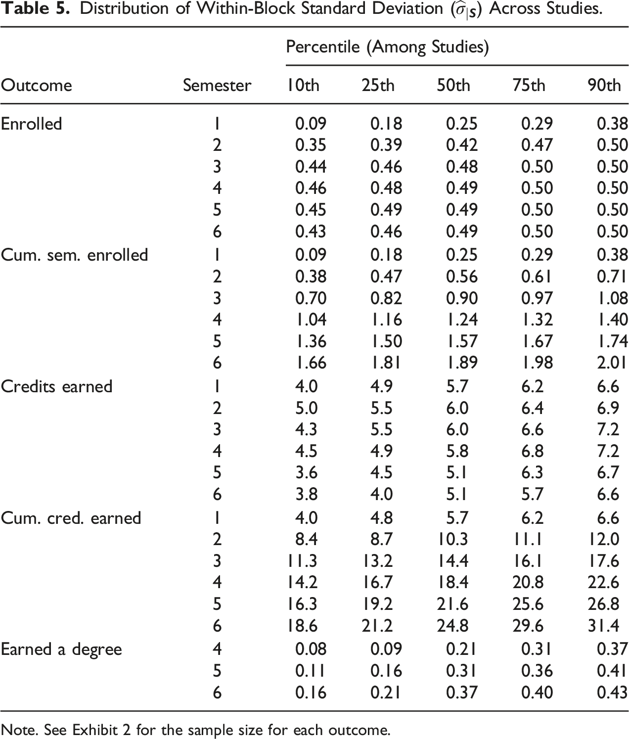
In this section, we present estimates of the within-block standard deviation ( ${\widehat{\sigma }}_{|\mathit{S}}$ ) for each of the main outcomes (enrollment, credits earned, and degree completion). We consider the extent that ${\widehat{\sigma }}_{|\mathit{S}}$ varies across semesters of follow-up and across RCTs, and discuss the implications of these patterns for the MDTE. Estimates of ${\widehat{\sigma }}_{|\mathit{S}}$ are summarized in Table 5. The key finding is that ${\widehat{\sigma }}_{|\mathit{S}}$ , and therefore the MDTE, increases over time for cumulative semesters enrolled and credits earned and that there can be substantial variation in estimates of the within-block standard deviation across studies (most notably, for enrollment in early semesters and for degree completion).

Table 5.

Distribution of Within-Block Standard Deviation ( ${\widehat{\sigma }}_{|\mathit{S}}$ ) Across Studies.

		Percentile (Among Studies)
Outcome	Semester	10th	25th	50th	75th	90th
Enrolled	1	0.09	0.18	0.25	0.29	0.38
	2	0.35	0.39	0.42	0.47	0.50
	3	0.44	0.46	0.48	0.50	0.50
	4	0.46	0.48	0.49	0.50	0.50
	5	0.45	0.49	0.49	0.50	0.50
	6	0.43	0.46	0.49	0.50	0.50
Cum. sem. enrolled	1	0.09	0.18	0.25	0.29	0.38
	2	0.38	0.47	0.56	0.61	0.71
	3	0.70	0.82	0.90	0.97	1.08
	4	1.04	1.16	1.24	1.32	1.40
	5	1.36	1.50	1.57	1.67	1.74
	6	1.66	1.81	1.89	1.98	2.01
Credits earned	1	4.0	4.9	5.7	6.2	6.6
	2	5.0	5.5	6.0	6.4	6.9
	3	4.3	5.5	6.0	6.6	7.2
	4	4.5	4.9	5.8	6.8	7.2
	5	3.6	4.5	5.1	6.3	6.7
	6	3.8	4.0	5.1	5.7	6.6
Cum. cred. earned	1	4.0	4.8	5.7	6.2	6.6
	2	8.4	8.7	10.3	11.1	12.0
	3	11.3	13.2	14.4	16.1	17.6
	4	14.2	16.7	18.4	20.8	22.6
	5	16.3	19.2	21.6	25.6	26.8
	6	18.6	21.2	24.8	29.6	31.4
Earned a degree	4	0.08	0.09	0.21	0.31	0.37
	5	0.11	0.16	0.31	0.36	0.41
	6	0.16	0.21	0.37	0.40	0.43

Note. See Exhibit 2 for the sample size for each outcome.

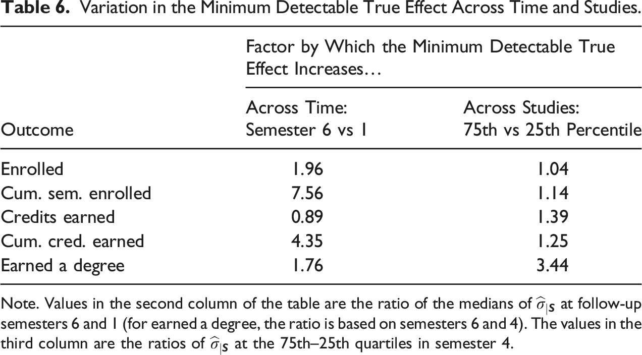
Before delving into these findings, two features of the standard deviation are worth emphasizing. First, recall from equations (2) and (3) that as ${\sigma }_{|S}$ decreases so does the standard error of the impact estimator and the MDTE. All else equal, the MDTE will change by the same proportion as the standard deviation; for example, a 50% reduction in ${\sigma }_{|S}$ will reduce the MDTE by 50% as well. Therefore, to frame the discussion of the findings, Table 6 shows the factor by which the MDTE increases from semester 1 to semester 6—and between studies in the 25th and 75th percentile—based on the estimates of ${\sigma }_{|\mathit{S}}$ in Table 5. (A factor of 1 would indicate that the MDTE are the same across time and studies; a factor of 2 would indicate that the MDTE is twice as large.)

Table 6.

Variation in the Minimum Detectable True Effect Across Time and Studies.

Outcome	Factor by Which the Minimum Detectable True Effect Increases…
	Across Time: Semester 6 vs 1	Across Studies:75th vs 25th Percentile
Enrolled	1.96	1.04
Cum. sem. enrolled	7.56	1.14
Credits earned	0.89	1.39
Cum. cred. earned	4.35	1.25
Earned a degree	1.76	3.44

Note. Values in the second column of the table are the ratio of the medians of ${\widehat{\sigma }}_{|\mathit{S}}$ at follow-up semesters 6 and 1 (for earned a degree, the ratio is based on semesters 6 and 4). The values in the third column are the ratios of ${\widehat{\sigma }}_{|\mathit{S}}$ at the 75th–25th quartiles in semester 4.

Second, for binary outcomes (enrollment and degree completion), it is useful to note that the shape of the relationship between the mean and standard deviation of the outcome is an inverted parabola. The standard deviation peaks when success rates are 50% and takes on smaller values as success rates move away from 50% toward 0% or 100%. As a result, to detect the same effect in percentage points (e.g., a 5-percentage point effect), a larger sample size is necessary when success rates are near 50% compared to if they are near 10% or 90%. Notably, this phenomenon moves very slowly as success rate move away from 50% (e.g., from 50% to 60%) compared with changes of the same size at more extreme levels (e.g., from 80% to 90%).

Enrollment

We consider two enrollment variables—a binary indicator of enrollment in each semester and the cumulative number of semesters enrolled through a given semester.

For the binary measure of enrollment in each semester of follow-up, looking across time the values of ${\widehat{\sigma }}_{|\mathit{S}}$ start small, in the 0.18–0.29 range in semester 1 (based on the 25th and 75th percentiles), and quickly increase before maxing out near 0.50. This is because in semester 1 enrollment levels are high—typically around 80–95%—and as noted earlier the standard deviation for binary outcomes is largest at 50% and smallest at 0% or 100%. As students stop out, drop out, or graduate, enrollment levels tend to decrease to the 40–60% range in semesters 4 and 5, resulting in a larger ${\widehat{\sigma }}_{|\mathit{S}}$ (and thus larger MDTE in percentage points). Beyond semester 6 we can expect ${\widehat{\sigma }}_{|\mathit{S}}$ to decrease (and the MDTE to fall with it), as more students stop out, drop out, or graduate and enrollment approaches 0%.

Looking across studies, the ${\widehat{\sigma }}_{|\mathit{S}}$ for enrollment in each semester varies substantially in semesters 1 and 2 but varies much less so in semesters 3–6. This is a result of the inverted parabolic relationship between the mean and standard deviation of binary variables. At the extremes (near 0 and 100% enrollment), small changes in the mean lead to big changes in the standard deviation. Thus, when enrollment is in the 80–95% range (i.e., the rates we tend to see in semester 1), ${\widehat{\sigma }}_{|\mathit{S}}$ varies a lot across studies. When enrollment is in the 40%–75% range (i.e., the rates we tend to see in semesters 4 and 5), ${\widehat{\sigma }}_{|\mathit{S}}$ takes on similar values across studies.

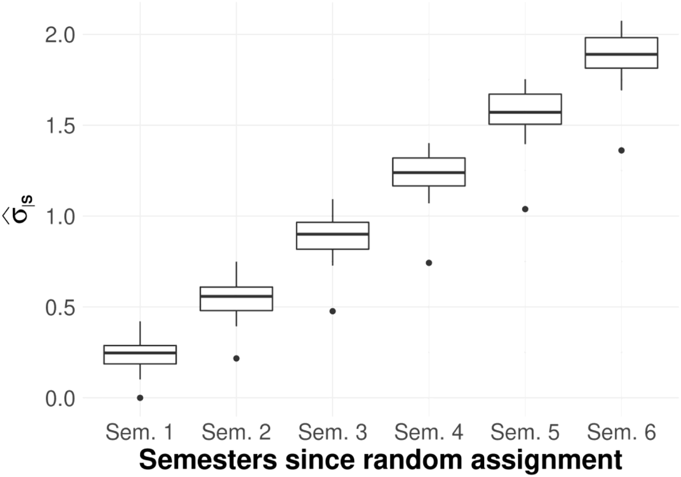
For cumulative semesters enrolled, looking across time the values of ${\widehat{\sigma }}_{|\mathit{S}}$ increase linearly from semester 1 to 6 (see Figure 1). This is because the distribution of cumulative semesters enrolled widens over time as the range of possible values expands. In semester 1, students have enrolled in 0 or 1 semesters, but by semester 6, students have enrolled in 0, 1, 2, 3, 4, 5, or 6 semesters. Across studies, the distribution of the ${\widehat{\sigma }}_{|\mathit{S}}$ for cumulative semesters enrolled is consistent over time, with a typical interquartile range of around 0.15.

Figure 1.

Box plot of ${\widehat{\sigma }}_{|\mathit{S}}$ for cumulative semesters enrolled at the end of each of six semesters. Note. The main analytic sample for this outcome includes 14 studies and 7028 students.

For the enrollment outcomes, the increase in ${\widehat{\sigma }}_{|\mathit{S}}$ over time has important implications for RCT design and interpretation. Across studies the median ${\widehat{\sigma }}_{|\mathit{S}}$ for enrollment in semester 6 is 0.49, which is 1.96 times larger than the median value in semester 1 (0.25). Hence the MDTE for semester 6 compared to semester 1 is also 1.96 times larger. As a concrete example, for an RCT where $J\overline{n}$ = 1,000, $\overline{T}$ = 0.50, $1-\beta$ = 0.80, $\alpha$ = 0.05, and $R_{|\mathit{S}}^2$ = 0.05, the MDTE would be a 4.3 percentage point effect on enrollment in semester 1 and 8.5 percentage point effect in semester 6. Most interventions aiming to improve persistence have larger effects in earlier semesters when precision is best. In later semesters, when enrollment impacts are typically smaller, precision gets worse. This is important to be aware of when planning a study and when interpreting findings. An estimated effect of the same magnitude can be statistically significant in semester 1 and no longer statistically significant in later semesters.

Total Credits Earned

We consider two credits earned variables—total credits earned in each semester and cumulative credits earned through a given semester. ²³

For credits earned in each semester, ${\widehat{\sigma }}_{|\mathbf{S}}$ tends to be in the four to seven credit range across studies. Across time, the values of ${\widehat{\sigma }}_{|\mathbf{S}}$ (and thus the MDTE) are shaped like an inverted “U”, with median values ranging from a minimum of 5.1 to a maximum of 6.0. Across studies within a given semester, the interquartile range of ${\widehat{\sigma }}_{|\mathbf{S}}$ tends to be between 1 and 1.7. Based on the same assumptions described above, if ${\sigma }_{|\mathrm{S}}$ is in the 4–7 range (covering a large proportion of our estimates for credits earned in each semester), the MDTE takes on a value 0.69 to 1.21 credits earned in a semester. This represents about 17–30% of students passing one more course than they would have otherwise (assuming four credit courses).

For cumulative credits earned, which is perhaps the most ubiquitous measure of academic progress, the values of ${\widehat{\sigma }}_{|\mathbf{S}}$ increase substantially from semester 1 to 6. Like cumulative semesters enrolled, this increase is a result of some students dropping out and others continuing to earn credits, expanding the range of cumulative credits earned over time. The median ${\widehat{\sigma }}_{|\mathit{S}}$ is 5.7 in semester 1 and it increases to 24.8 in semester 6. This implies that the MDTE for cumulative credits earned in semester 6 is more than 4 times larger (=24.8/5.7) than the MDTE in semester 1. An important implication is that early statistically significant impacts on cumulative credits earned can become statistically insignificant in later semesters of follow-up, even when their magnitude remains constant or even increases, as in Scrivener and Weiss (2009). This may create the false impression that effects on cumulative credits earned “fade-out” in postsecondary studies, when the evidence shows otherwise (Weiss et al., 2021).

Degree Completion

Most evaluations of programs designed for community college students do not seriously consider effects on degree completion until the end of year 2 (semester 4). With respect to degree completion (a binary outcome), ${\widehat{\sigma }}_{|\mathit{S}}$ increases from the end of 2 years (i.e., four semesters) to the end of 3 years (i.e., six semesters). This increase corresponds with the increase in graduation rates, which approach but do not cross the 50% threshold in that timeframe.

Strikingly, for the degree completion outcome there is substantial variation in ${\widehat{\sigma }}_{|\mathit{S}}$ across studies, proportionally more so than for other outcomes. For example, at the end of 2 years the first quartile is 0.09 and the third quartile is 0.31, corresponding with cross-study variation in rates of degree completion. This means the MDTE in some studies is almost four times larger (=0.31/0.09) than in other studies.

Empirical Estimates of the Proportion of Outcome Variation Explained by Covariates ( ${\mathit{R}}_{|\mathit{S}}^2$ )

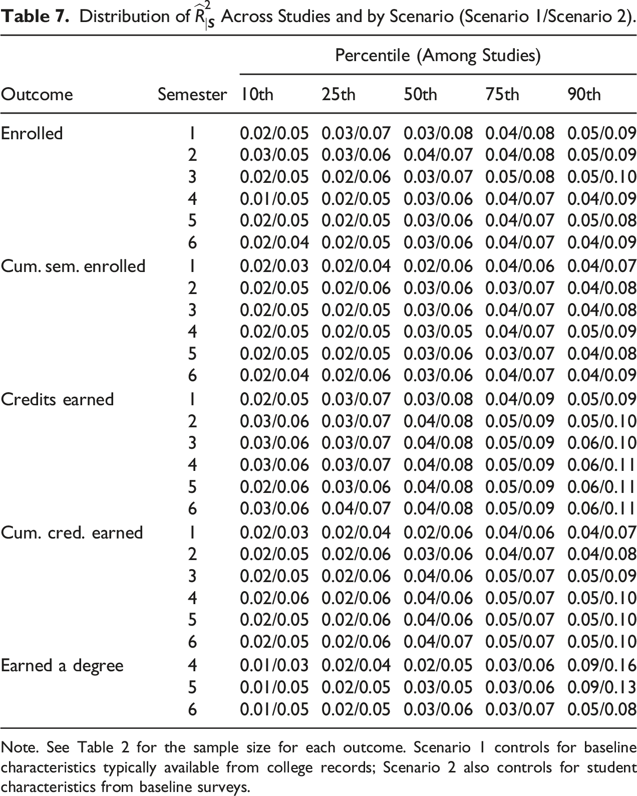
In this section, we present estimates of the proportion of the outcome variance explained by covariates within blocks ( ${\widehat{R}}_{|\mathit{S}}^2$ ) for each of the main outcomes (enrollment, credits earned, and degree completion). Estimates of $R_{|\mathit{S}}^2$ were generated for different scenarios that reflect the types of baseline covariates that may be available to researchers. Recall that the MDTE decreases as the proportion of outcome variation explained by the baseline covariates ( $R_{|\mathit{S}}^2$ ) increases. Estimates of $R_{|\mathit{S}}^2$ are summarized in Table 7.

Table 7.

Distribution of ${\widehat{R}}_{|\mathit{S}}^2$ Across Studies and by Scenario (Scenario 1/Scenario 2).

		Percentile (Among Studies)
Outcome	Semester	10th	25th	50th	75th	90th
Enrolled	1	0.02/0.05	0.03/0.07	0.03/0.08	0.04/0.08	0.05/0.09
	2	0.03/0.05	0.03/0.06	0.04/0.07	0.04/0.08	0.05/0.09
	3	0.02/0.05	0.02/0.06	0.03/0.07	0.05/0.08	0.05/0.10
	4	0.01/0.05	0.02/0.05	0.03/0.06	0.04/0.07	0.04/0.09
	5	0.02/0.05	0.02/0.05	0.03/0.06	0.04/0.07	0.05/0.08
	6	0.02/0.04	0.02/0.05	0.03/0.06	0.04/0.07	0.04/0.09
Cum. sem. enrolled	1	0.02/0.03	0.02/0.04	0.02/0.06	0.04/0.06	0.04/0.07
	2	0.02/0.05	0.02/0.06	0.03/0.06	0.03/0.07	0.04/0.08
	3	0.02/0.05	0.02/0.05	0.03/0.06	0.04/0.07	0.04/0.08
	4	0.02/0.05	0.02/0.05	0.03/0.05	0.04/0.07	0.05/0.09
	5	0.02/0.05	0.02/0.05	0.03/0.06	0.03/0.07	0.04/0.08
	6	0.02/0.04	0.02/0.06	0.03/0.06	0.04/0.07	0.04/0.09
Credits earned	1	0.02/0.05	0.03/0.07	0.03/0.08	0.04/0.09	0.05/0.09
	2	0.03/0.06	0.03/0.07	0.04/0.08	0.05/0.09	0.05/0.10
	3	0.03/0.06	0.03/0.07	0.04/0.08	0.05/0.09	0.06/0.10
	4	0.03/0.06	0.03/0.07	0.04/0.08	0.05/0.09	0.06/0.11
	5	0.02/0.06	0.03/0.06	0.04/0.08	0.05/0.09	0.06/0.11
	6	0.03/0.06	0.04/0.07	0.04/0.08	0.05/0.09	0.06/0.11
Cum. cred. earned	1	0.02/0.03	0.02/0.04	0.02/0.06	0.04/0.06	0.04/0.07
	2	0.02/0.05	0.02/0.06	0.03/0.06	0.04/0.07	0.04/0.08
	3	0.02/0.05	0.02/0.06	0.04/0.06	0.05/0.07	0.05/0.09
	4	0.02/0.06	0.02/0.06	0.04/0.06	0.05/0.07	0.05/0.10
	5	0.02/0.05	0.02/0.06	0.04/0.06	0.05/0.07	0.05/0.10
	6	0.02/0.05	0.02/0.06	0.04/0.07	0.05/0.07	0.05/0.10
Earned a degree	4	0.01/0.03	0.02/0.04	0.02/0.05	0.03/0.06	0.09/0.16
	5	0.01/0.05	0.02/0.05	0.03/0.05	0.03/0.06	0.09/0.13
	6	0.01/0.05	0.02/0.05	0.03/0.06	0.03/0.07	0.05/0.08

Note. See Table 2 for the sample size for each outcome. Scenario 1 controls for baseline characteristics typically available from college records; Scenario 2 also controls for student characteristics from baseline surveys.

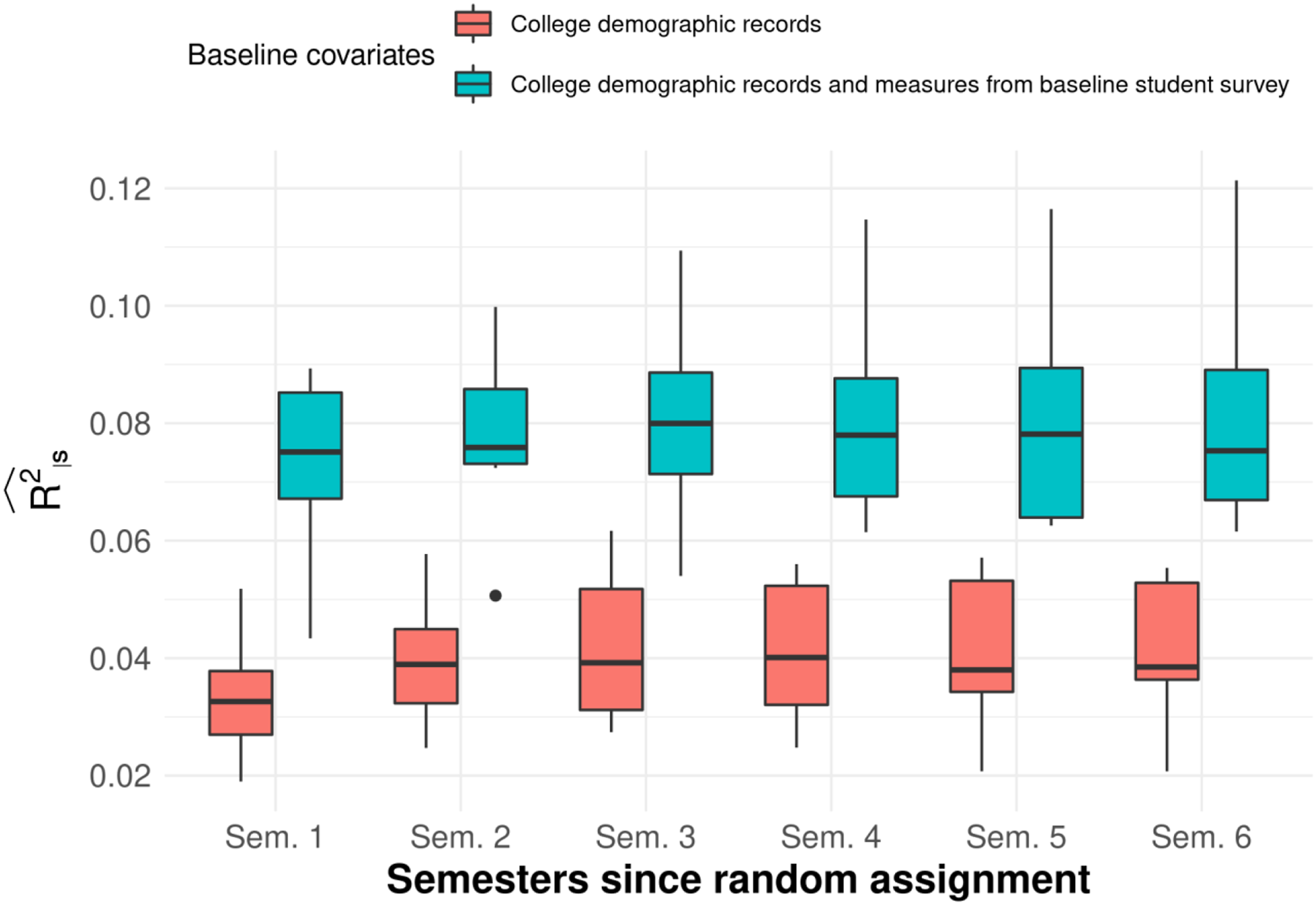
The key finding is that estimates of the $R_{|\mathit{S}}^2$ are quite small across all outcomes examined here, especially when compared to the pretest-posttest relationships often seen in the K-12 literature (e.g., Bloom et al., 2007; Hedges & Hedberg, 2014). Values are less than 0.10, regardless of the types of covariates included in the model. Two patterns—or rather, the lack thereof—are notable: (1) controlling for baseline covariates collected through surveys does not meaningfully increase the ${\widehat{R}}_{|\mathit{S}}^2$ , and (2) the ${\widehat{R}}_{|\mathit{S}}^2$ is stable across the first six semesters of follow-up and does not decrease as one might expect given that outcomes typically are harder to predict as one goes further into the future. (This pattern of findings is illustrated in Figure 2 for cumulative credits earned.)

Figure 2.

Box plot of $R_{|\mathit{S}}^2$ for cumulative credits earned at the end of each semester, by type of baseline covariate. Note. The main analytic sample for this outcome includes 8 studies and 5649 students.

When only covariates available from college demographic records are used (Scenario 1), ${\widehat{R}}_{|\mathit{S}}^2$ generally falls between 0.02 and 0.05 for all the outcomes and time periods examined. There are no noticeable trends over time for any outcome, suggesting that however little explanatory power the covariates have is maintained over the first six semesters. There does not appear to be much variation across interventions, either: the spread between the 10^th percentile and 90^th percentile rarely exceeds 0.05.

When a richer set of covariates from baseline surveys are also used (Scenario 2), estimates of $R_{|\mathit{S}}^2$ are higher as expected but still consistently small, typically between 0.05 and 0.08. This suggests that collecting additional demographic information may yield an increase in explanatory power that is too small to meaningfully reduce the MDTE. For example, for an RCT where $J\overline{n}$ = 1,000, $\overline{T}$ = 0.50, 1- $\beta$ = 0.80, $\alpha$ = 0.05, and ${\sigma }_{|S}$ =5.69 (the median in semester 1), the MDTE for the effect on cumulative credits earned decreases from 0.98 to 0.96 when $R_{|\mathit{S}}^2$ increases from 0.05 to 0.10.

As a supplemental analysis (based on a smaller subset of studies), we also examined whether controlling for placement test scores as covariates (in addition to college demographic records) increases $R_{|\mathit{S}}^2$ . However, the gain in ${\widehat{R}}_{|\mathit{S}}^2$ from adding placement test covariates is roughly the same as adding the survey covariates: quite small. Overall, these findings are similar to those from the literature on placements tests as a predictor of students’ college performance; Belfield and Crosta (2012) find that college placement tests explain only 6% of the variation in credits earned.

Overall, the small values of ${\widehat{R}}_{|\mathit{S}}^2$ across the board indicate that in CC studies, the explanatory power of the kinds of baseline covariates examined in the present analysis may not be large enough to appreciably reduce sample size requirements. For example, all else equal, a set of covariates that yield an $R_{|\mathit{S}}^2$ of 0.05 would reduce the sample requirements by 5%, or 50 students in a 1000-student study, relative to no covariates. The results from this paper also confirm that CC researchers should not use $R_{|\mathit{S}}^2$ assumptions from K-12 studies, which tend to be much larger. The main reason is likely that K-12 studies often rely on a pre-test covariate and a post-test outcome measure—such measures are often aligned with each other, continuous, and reliable, thus yielding high explanatory power. ²⁴

Design Parameters for College Grade Point Average

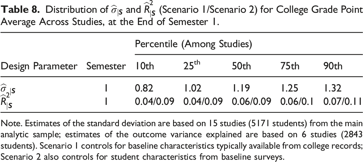
This section discusses the design parameters for college GPA. As discussed earlier college GPA is not typically a primary outcome in community college studies because it can only be measured for students who remain enrolled, so we focus here only on parameter estimates at the end of the first semester (Table 8). ²⁵

Table 8.

Distribution of ${\widehat{\sigma }}_{|\mathit{S}}$ and ${\widehat{R}}_{|\mathit{S}}^2$ (Scenario 1/Scenario 2) for College Grade Point Average Across Studies, at the End of Semester 1.

		Percentile (Among Studies)
Design Parameter	Semester	10th	25th	50th	75th	90th
${\widehat{\sigma }}_{|\mathit{S}}$	1	0.82	1.02	1.19	1.25	1.32
${\widehat{R}}_{|\mathit{S}}^2$	1	0.04/0.09	0.04/0.09	0.06/0.09	0.06/0.1	0.07/0.11

Note. Estimates of the standard deviation are based on 15 studies (5171 students) from the main analytic sample; estimates of the outcome variance explained are based on 6 studies (2843 students). Scenario 1 controls for baseline characteristics typically available from college records; Scenario 2 also controls for student characteristics from baseline surveys.

With respect to the within-block standard deviation, the median estimate across studies is 1.19. Though there is variation across studies, the amount of variation is the smallest of any outcome examined in this paper for the first semester.

Like the other outcomes examined in this paper, the variance in college GPA explained by baseline covariates is small—the median estimate is 0.06 (Scenario 1) and 0.09 (Scenario 2)—and controlling for placement tests does not appreciably increase ${\widehat{R}}_{|\mathit{S}}^2$ . These findings are similar to those from prior studies of placement tests as predictors of college performance. Belfield and Crosta (2012) find that college placement tests explain only 5% of the variation in college GPA. Similarly, Scott-Clayton (2012) finds that placement tests explain about 2% of the variation in students’ grades in their first college-level English course, and 13% of the variation in students grades in their first college-level course in Math.

Conclusion

The findings from this paper highlight several important lessons for planning RCTs in a community college setting. Importantly, these lessons differ substantively from the guidance for planning K-12 studies, so as intended, the present paper’s findings fill an important gap with respect to planning well-powered RCTs of interventions delivered to community college students.

First, researchers should be mindful of the follow-up period when planning their study. For cumulative semesters enrolled and credits earned, ${\sigma }_{|S}$ (and the MDTE) can be larger in later semesters—4.4 to 7.6 times larger in follow-up semester 6 than semester 1 for these outcomes. This makes it especially important for researchers to select design parameters that align with the time period of their key research questions. Ideally, researchers should power their study based on the latest follow-up semester given their research questions. For studies of interventions whose effects do not increase over time, however, doing so will likely require recruiting a larger sample of students, which may not always be possible. If powering the study based on later semesters is not feasible, then estimated effects that were statistically significant in early semesters may become statistically insignificant in later semesters even if their magnitude is the same or larger—a pattern caused by the “fuzz out” of effects rather than their “fade out”. To disentangle these explanations for non-significant findings in later semesters, researchers should estimate effects in early semesters—and compare them to the magnitude of effects in later semesters—to aid with interpretation. More generally, even if longer-term effects “fuzz out”, there can still be value to underpowered longer-term findings because they can contribute to knowledge-building if they are included in meta-analyses.

Second, when planning CC RCTs, researchers should consider that there can be substantial variation in ${\sigma }_{|S}$ (and the MDTE) across settings, making it tricky to pin down a value to plug in for MDTE calculations. This can be especially true for enrollment outcomes in early semesters as well as degree completion. For these outcomes, the MDTE is 3–4 times larger when assumptions about ${\sigma }_{\Vert \mathit{S}}$ are based on the 75th quartile in the distribution compared to the 25th percentile. This variation may be a result of the context of the study, the population targeted, or other factors. In those circumstances, it is probably worth choosing a range of ${\sigma }_{|\mathit{S}}$ values (e.g., the 25th and 75th percentiles from this paper) and then making study design decisions based on factors like cost, feasibility of recruiting larger samples, and tolerance for greater uncertainty.

Given the substantial variation in ${\sigma }_{|\mathit{S}}$ across studies for some outcomes, researchers could also consider leveraging extant data to obtain a better estimate for their target population. For example, during the planning phase, estimates of outcome variation could be obtained from the study colleges based on data for current or previous students who are eligible for the intervention. For binary outcomes, another source of information are publicly available datasets; the Integrated Postsecondary Education Data System (IPEDS), for example, includes mean levels for some binary outcomes (like graduation rates) at the college level and for student subgroups, which can be used to derive the standard deviation of these outcomes. ²⁶ Using publicly available data sources is especially suitable when all eligible students will be participating in the study and the target population aligns with the population examined in IPEDS. ²⁷ If the sample for a planned study will include a self-selected group of students whose outcomes may vary from the general or eligible population at the college—and if the study will include multiple cohorts—another option is to update the expected MDTE at the end of the first study year based on parameters estimates for the first cohort, to determine whether the planned sample size is sufficient or whether additional (or fewer) cohorts should be recruited.

The third lesson from this paper is that the kinds of baseline covariates that are typically available from surveys and college records are likely to explain very little of the variation in student outcomes. When planning a study, researchers should assume a very low or null value for ${\mathrm{R}}_{|\mathit{S}}^2$ , in the range of 0–0.05. Unlike K-12 studies, where the outcomes of interest (like test scores) can also be measured at baseline, covariates in CC studies cannot be relied upon to meaningfully reduce the MDTE. Hence, researchers’ plans for collecting baseline data for a study should be based on considerations related to describing the sample, establishing baseline similarity between their treatment and control groups, and defining student subgroups—as opposed to improving the precision of estimated effects.

Ideally, this paper will eventually be one of many future studies providing guidance to researchers on planning RCTs in community college settings. Over time, the empirical literature on K-12 design parameters has grown to include estimates from several states and for different study designs. Similarly, as the number of CC studies increases, there will be opportunities to supplement the findings from this paper with estimates from additional colleges and sites, and to examine unanswered but important questions.

One limitation of our analysis—which future studies may address—is whether controlling for students’ high school outcomes could meaningfully increase the ${\mathrm{R}}_{|\mathit{S}}^2$ . For example, Belfield and Crosta (2012) find that high school GPA explains 21% and 14% of the variation in college GPA and credits earned, respectively. Although these larger ${\mathrm{R}}_{|\mathit{S}}^2$ may still not appreciably affect the MDTE, ²⁸ the extent to which high school transcript data can improve the precision of estimated effects on college outcomes warrants examination with additional datasets, including studies where the target population is prospective students or applicants. Similarly, another avenue to explore—relevant to studies where the target population is continuing students—is the explanatory power of GPA and credits earned by students in prior semesters.

Another key question not addressed by this paper is the magnitude of effects that CC studies should be powered to detect. For example, is an MDTE of 5 percentage points on graduation rates achievable or should the study be powered to detect even smaller effects? The effect of an intervention depends on several factors including the context (the setting and target population); the design of the intervention and how well it is implemented; how different it is from “business as usual”; and the amount of intervention received by students. In the context of K-12 interventions, national and study-specific datasets have been used to generate useful benchmarks for achievable and policy-relevant effect sizes (Bloom, Hill et al., 2008; Hill et al., 2008; Kraft, 2020). Similar benchmarks are needed to guide the planning of evaluations of interventions implemented in community colleges. We plan to tackle this issue in forthcoming research.