Sage Journals: Discover world-class research

Abstract

Attrition in longitudinal studies is a major threat to the representativeness of the data and the generalizability of the findings. Typical approaches to address systematic nonresponse are either expensive and unsatisfactory (e.g., oversampling) or rely on the unrealistic assumption of data missing at random (e.g., multiple imputation). Thus, models that effectively predict who most likely drops out in subsequent occasions might offer the opportunity to take countermeasures (e.g., incentives). With the current study, we introduce a longitudinal model validation approach and examine whether attrition in two nationally representative longitudinal panel studies can be predicted accurately. We compare the performance of a basic logistic regression model with a more flexible, data-driven machine learning algorithm—gradient boosting machines. Our results show almost no difference in accuracies for both modeling approaches, which contradicts claims of similar studies on survey attrition. Prediction models could not be generalized across surveys and were less accurate when tested at a later survey wave. We discuss the implications of these findings for survey retention, the use of complex machine learning algorithms, and give some recommendations to deal with study attrition.

Keywords

Machine learning attrition longitudinal studies predictive modeling generalizability

Data of longitudinal panel surveys constitute an important resource for educational, psychological, sociological, and health-related research (e.g., Behr et al., 2020; Rackoff & Newman, 2020). In contrast to cross-sectional data, longitudinal data allow to study developmental trajectories or within-person change in addition to between-person differences (Voelkle et al., 2014). However, the strength of longitudinal designs—assessing the same individuals at multiple occasions—also entails the risk of attrition, which is defined as temporary or permanent dropout of participants. High attrition rates are a major problem in longitudinal research affecting the validity of conclusions drawn from such data (Schoeni et al., 2012). More precisely, systematic dropout of participants sharing common characteristics (e.g., low socioeconomic status) renders the remaining sample unrepresentative, which in turn can lead to biased results (Heffetz & Reeves, 2019; Little & Rubin, 2002). For example, a longitudinal study on the effects of counseling on depression in which participants with the highest depression scores are most likely to drop out of the sample would falsely indicate a therapy to be more effective (Nicholson et al., 2017).

With the current study, we try to predict attrition using data-driven machine learning algorithms. Insights about relevant predictors can then be used to take potentially more effective measures to anticipate and prevent attrition such as targeted incentives for at-risk participants (Lynn, 2017; Pforr et al., 2015). We compare the predictive accuracy of logistic regressions models with a machine learning algorithm, namely, gradient boosting machines (GBM; Friedman, 2001) in two longitudinal panel studies: Midlife in the United States (MIDUS) and Panel Analysis of Intimate Relationships and Family Dynamics (pairfam). Finally, we evaluate our results in terms of generalizability across studies and survey waves, respectively.

Strategies in Dealing With Panel Attrition

In the following, we will shortly present methods that are used to ensure the representativeness of the sample—(a) statistical modeling, (b) poststratification weights, or (c) oversampling/refreshment samples—and discuss their strengths and limitations. First, to address wave nonresponse, that is, participants’ data completely missing for a study wave in longitudinal studies, one could use the same procedures that are recommended in the missing data literature for item nonresponse (e.g., Enders, 2010; Little & Rubin, 2002). However, imputation-based or model-based approaches rely on the assumption of missing at random (Schafer & Graham, 2002), that is, the occurrence of missing values does not depend on the expression of the variable itself or on the expression of other variables in the data set after controlling for other observed variables. This prerequisite is problematic, as participants’ most likely drop out systematically (missing not at random) and variables that are associated with this process are often unknown in advance or difficult to measure. However, recently promising approaches on handling non-random missing data have been developed (for an overview, see Kleinke et al., 2020; Van Buuren, 2018). Researchers often try to reduce potential bias by incorporating relevant auxiliary variables in multiple imputation that might produce robust results despite common concerns (Mustillo & Kwon, 2014), but not in all cases (Hardt et al., 2012). Simpler methods such as listwise or pairwise deletion are used regularly and often lead to biased estimates (Jeličić et al., 2009).

A second approach to compensate for attrition bias is to use poststratification weights. Groups or individuals are assigned weights according to their inversed probability of participation (Seaman & White, 2013). Thus, the usefulness of weighting hinges on whether all relevant predictors of attrition are integrated into the statistical model that is used to calculate these probabilities (Gelman, 2007). As weighting does not replace missing values and requires complete data, any occurring item nonresponse must be addressed beforehand (e.g., using multiple imputation). Consequently, the later waves’ sample sizes of a longitudinal study still lack statistical power. Also, weights often lead to an increased variance of estimators (Schmidt & Woll, 2017) and must be adjusted depending on which study waves or variables are analyzed.

A third approach is oversampling, which refers to the countermeasure of recruiting more participants who are likely to drop during a longitudinal study. Oversampling recognizes attrition as inevitable and tries to buffer the unavoidable unrepresentativeness of the data and to reduce selection bias by starting with an unbalanced sample at baseline. Following a similar logic, refreshment samples consist of new participants added at subsequent measurement occasions that are often sampled using the same sampling procedure as for the initial recruitment (Deng et al., 2013). Whereas additional participants generally enhance statistical power, it has been advised to select refreshment participants who share characteristics with nonrespondents to avoid introducing bias (Dorsett, 2010). Additional negative aspects of using oversampling or refreshment samples are their high costs and that they often not sufficiently compensate bias and therefore have to be combined with other strategies.

Drawbacks of Common Approaches to Analyzing Panel Attrition

Previous studies often examined attrition with different variables that are routinely collected at baseline such as demographic variables using logistic regressions (Eisner et al., 2018). This research repeatedly reported that males, singles, people with migration background, less educated, and urban living participants are at higher risk of becoming nonrespondents (Radler & Ryff, 2010; Young et al., 2006). Given that longitudinal studies usually focus on a specific topic and that panels are time-restricted, the breadth and depth of these variables are somewhat limited. But it is plausible to assume that the decision to (regularly) take part in longitudinal studies can be influenced by several factors beyond demographics such as personality (e.g., Lugtig, 2014) or health (e.g., Jacobsen et al., 2021). However, studies on personality or health focus on specific sets of variables, neglecting others.

Taken together, the selection and quantity of predictors used in previous research to predict attrition are often limited. Moreover, the assumption of exclusively linear effects on attrition is questionable. Radler and Ryff (2010) showed that, for example, age interacted with subjective health when predicting attrition in the second study wave of MIDUS: Elderly participants only had a higher attrition probability when they also rated their subjective health as poorly, whereas older participants in excellent health showed significantly lower attrition rates. Not addressing such interaction effects may result in less accurate models.

Another common drawback of traditional attrition modeling approaches is that it is unclear whether their results are generalizable. The ability of a model to provide accurate and generalizable predictions is especially essential in applied research (Rocca & Yarkoni, 2020; Shmueli, 2010) such as study retention. To enable panel administrators to employ effective retention strategies (e.g., person-specific incentives at future waves), a prediction model also has to hold in future waves. In general, to quantify the unbiased predictive accuracy, any model must be evaluated on new data, which is often achieved by splitting a data set into a training-validation and a testing data set. However, the question whether a model predicting attrition will also hold in future waves or across different longitudinal studies goes beyond this form of internal cross-validation. Rather, it aims at the generalizability of the results. Generalizability concerns the extent to which the study results apply across different items assessing the same construct (item sampling), across different participants (person sampling), across different measurement occasions (time sampling), and across different analytical methods (method sampling). As these aspects of longitudinal testing are of particular interest for study planning, researchers should ask to what extent their prediction models generalize across them.

Predicting Panel Attrition Using Machine Learning

A few recent studies have picked up on the notion of temporally validating their models of attrition and including nonlinear and interaction effects by using machine learning algorithms to predict attrition in longitudinal studies (Jacobsen et al., 2021; Kern et al., 2019; Zinn & Gnambs, 2020). Machine learning algorithms are often recommended to efficiently deal with extensive data, collinearity of predictors, and complex relations between predictors and outcomes (e.g., Zou & Hastie, 2005). The assumption in these studies is that the reasons for participants to drop are complex and that the complexity of the method should match this causal complexity. For example, Kern et al. (2019) used different sets of predictors with various machine learning algorithms to predict attrition in a longitudinal German panel study. To validate their prediction models, the authors performed temporal cross-validation, which consisted of the following steps: A prediction model was built using data of all participants present at Wave 1 to predict the participation status at Wave 2. The resulting model is then tested using all active participants of Wave 2 to predict participation status at Wave 3. This validation approach was repeated for all 18 survey waves.

Using baseline variables and information on previous response behavior, a random forest algorithm achieved the highest predictive accuracy with an average area under the curve (AUC) of .875.¹ However, these promising results must be taken with a grain of salt. First, participants were automatically excluded from the panel when they were inactive for three waves in a row which is problematic because the outcome is logically dependent on a set of predictors, leading to inflated accuracies. Second, due to the temporal cross-validation scheme, most participants in the training data remain in the test data at later waves. Although this might seem justified at first glance since the study results do not have to generalize to other participants outside the given study sample, from a statistical point of view, an overlap of participants in training and test data leads to inflated accuracies, especially for tree-based algorithms (e.g., Jacobucci et al., 2021).

The Present Study

The present study has three main objectives: First, we aim to empirically test the notion that attrition can be predicted more accurately by means of machine learning algorithms that are able to incorporate nonlinear or interaction effects of heterogeneous predictors. To this end, we compare the predictive accuracy of a tree-based machine learning algorithm, GBM, and a logistic regression model. GBM sequentially combine multiple single decision trees that usually have a comparably poor predictive accuracy (Breiman, 2001). One advantage of GBM is that researchers do not have to a priori parameterize the relationship between an outcome and its predictors, which makes them popular for supervised classification tasks (e.g., Schroeders et al., 2022).

Second, we are interested in the longitudinal predictive accuracy of models on attrition. To validate prediction models, we employ a temporal validation approach with strictly disjoint training and testing data. This model validation strategy represents a stricter and more realistic test of predictive accuracy for future survey waves that are not bound to a specific group of participants. The third goal of this study is to tackle this issue of generalizability. Thus, we compare the prediction of attrition across two longitudinal large-scale studies that differ greatly in their study aims, sample, time frame: While one study is primarily concerned with midlife development of health and well-being in the United States with one wave every 9 years, the other is an annual German survey on partnership and family dynamics. Both studies measure similar constructs in their baseline assessment albeit sometimes using slightly different items. In terms of dimensions of generalizability, the items, persons, and time frame differ to a substantial degree allowing to gauge the generalizability of results across studies.

Method

Sample and Design

MIDUS

MIDUS is an American national survey carried out by the MacArthur Midlife Research Network (Brim et al., 2004). Each survey wave consists of a phone interview and additional questionnaires that participants have to send back. Starting in 1995, there was a random digit dialing sample of 4,244 participants as well as siblings of some of these participants (N = 950) and a twin sample (N = 1,914). Subsequent survey waves of MIDUS were conducted 9 years later in 2004 (second wave) and in 2013 (third wave). More information about MIDUS and the data of the first three waves can be found at http://www.midus.wisc.edu/data/. We consider participants as responding if they completed all parts of a survey wave. Therefore, we only use the subset of participants who completed all parts of survey at the first study wave (N = 6,325).

Pairfam

Pairfam is an annually conducted national survey on partnership and family dynamics in Germany (Huinink et al., 2011). It started in 2008 with a sample of 12,402 participants from three age cohorts (1971–1973, 1981–1983, and 1991–1993). Information about the participants are gathered via computer-assisted personal interviewing. Participants who were nonresponding in a previous wave, but did not explicitly decline their participation, are contacted again. After two nonresponses in a row, participants are excluded from the panel. The scientific use file and more information can be accessed at https://www.pairfam.de/. The following analyses were conducted on a subset of N = 11,875, because we excluded 527 participants with implausible values (BMI > 50).

Measures

We used core demographics, health, and personality related variables that have been shown to correlate with longitudinal attrition in previous studies and were available at baseline, except for personality in the pairfam study (see Supplemental Table S1 at https://osf.io/usjr7/). All categorical variables were dummy coded prior to the analysis using the first category as reference. The outcome participation status was dichotomously coded, irrespective of the reason.

Statistical Analyses

The current analyses are prediction models based on logistic regressions and gradient boosted machines. Irrespective of the algorithm, one important issue of any prediction is to reduce overfit, that is, to reduce the tendency of “statistical models to mistakenly fit sample-specific noise as if it were signal” (Yarkoni & Westfall, 2017, p. 3) while obtaining the highest predictive accuracy possible. To quantify the “true” or unbiased predictive accuracy, any prediction model has to be evaluated on new data—also called test data or withhold sample (Rocca & Yarkoni, 2020; Yarkoni & Westfall, 2017). Validating a prediction model with new data of an independent study is the most rigorous way of testing its generalizability (Dwyer et al., 2018). However, this is not always a feasible option and researchers often resort to workarounds such as multiple splitting their data into a training and testing data set to obtain robust estimates that resolve overfitting.

We used the following two validation strategies for the first three survey waves of MIDUS and pairfam, respectively: First, we ignored the temporal aspect of predicting future events and split the data into training data (80%) and testing data (20%; see the upper part of Figure 1), that is, training and testing the predictive model was done using the same measurement occasion (Wave 2). Second, we added a temporal validation strategy in which the aforementioned splitting of the data in strictly disjoint training and testing data is combined with temporal model validation (see the lower part of Figure 1). More precisely, we trained the model on 80% of the data at Wave 1 to predict status at Wave 2 and tested the resulting model using the active participants of the remaining 20% at Wave 2 to predict participation status at Wave 3. In doing so, we avoided any overlap of training and testing data and were also able to validate the prediction of the participation status of a future Wave 3.

Figure 1.

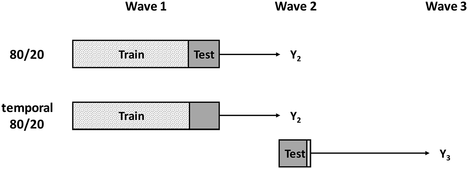
Different Cross-Validation Approaches in a Longitudinal Study Context. Excluded participants at Wave 2 are represented by the white section of the rectangle.

To avoid biased predictions due to highly unbalanced data, we used up-sampling to match the sample size of nonrespondents to respondents in the training data. The testing data were not affected by this procedure. Missing values were imputed separately for the training and testing data (i.e., after the 80/20 split) using the k-nearest neighbors algorithm implemented in caret. Nearest neighbor imputation procedures are hot-deck imputations in which a given number (k) of observations that are similar to the observation with a missing value (according to a distance metric, in this analysis the Euclidean distance) are used to replace missing values (e.g., Beretta & Santaniello, 2016). We used the default settings for imputation which were mean values of k = 5. For training the models, we used 10-fold cross-validation. To evaluate the classification into respondents and nonrespondents, we report balanced accuracy, that is, the mean of sensitivity and specificity. Sensitivity represents the ratio of correctly identified nonrespondents to all nonrespondents; specificity represents the ratio of correctly identified respondents to all respondents. Balanced accuracy was calculated for each testing data set of the 1,000 iterations.

All analyses were conducted using the R package caret (Kuhn, 2008) as an interface for modeling and prediction. We compared the predictive accuracy of a logistic regression and the GBM algorithm of the R package gbm (Version 2.1.5; Greenwell et al., 2019). We used the following default settings for the gbm tuning parameters: interaction depth of 1, 2, or 3; a minimum leaf size of 10; a shrinkage of .10; and number of trees 50, 100, or 150. As a sensitivity check of so-called hyperparameters on study results, we compared the default settings with a larger grid (interaction depth of 1, 2, 3, or 4, a minimum leaf size of 10, 20, or 50, a sequence of shrinkage values between .001 and .201 using steps of .01, and the number of trees 50, 100, 150, 300, or 500). The overall number of combinations in the larger grid was 1,260 as opposed to nine in the default settings. Considering that we split the data 1,000 times, we estimated 1,260,000 models with the larger grid compared with 9,000 with the default grid. Supplemental Figure S1 (see at https://osf.io/usjr7/) shows the balanced accuracies for MIDUS and pairfam and both validation strategies for both grids. The results show that the larger grid did not lead to any substantial improvement in the predictive accuracy. Thus, we focus the presentation and discussion of our results on those of the default grid. Annotated analyses scripts are available at https://osf.io/usjr7/.

Results

Following a suggestion of an anonymous reviewer, we checked whether the quality of the data at hand is eligible to be analyzed with the proposed methods. Results of this kind of “prestudy” showed that the data can be analyzed with logistic regression and GBM, that is, that the prediction accuracy can be reproduced given a known missing procedure. More information on these analyses can be found in a supplement in the OSF project at https://osf.io/usjr7/.

Both samples differ with respect to persons studied, items administered, and time frame considered. For example, participants of MIDUS were on average 21 years old, had an 11 percentage points lower share of migration background, and were more than twice as likely married than participants of the pairfam study. Education level and occupation status were measured differently across both studies and MIDUS had more information on chronic health conditions and personality than pairfam. With respect to attrition, in MIDUS 38% dropped from first to second wave (i.e., 2,396 of initially 6,325 participants) and another 20% from the second to third wave (1,283). In pairfam, 27% dropped out from first to second wave (i.e., 3,174 of the initial 11,875 participants) and another 9% from second to third wave. We provide an extensive Supplemental Table S1 showing descriptive statistics of all predictor variables for MIDUS and pairfam, respectively, and correlation plots of all predictor variables and participation status in the OSF project.

Figure 2 shows the balanced accuracies of 1,000 iterations for the logistic regressions and the GBM models for both studies and both validation approaches. Overall, it was not possible to accurately differentiate between nonrespondents and respondents. In the following, we will consider the results of the traditional 80/20 validation approach first. The amount of overfit (i.e., difference in the balanced accuracies between training and testing sample) was less pronounced for the logistic regressions (a difference in balanced accuracies of <.01 for MIDUS and .01 for pairfam) than for the GBM (.04 for MIDUS and .03 for pairfam). In general, both algorithms yielded almost identical balanced accuracies.

Figure 2.

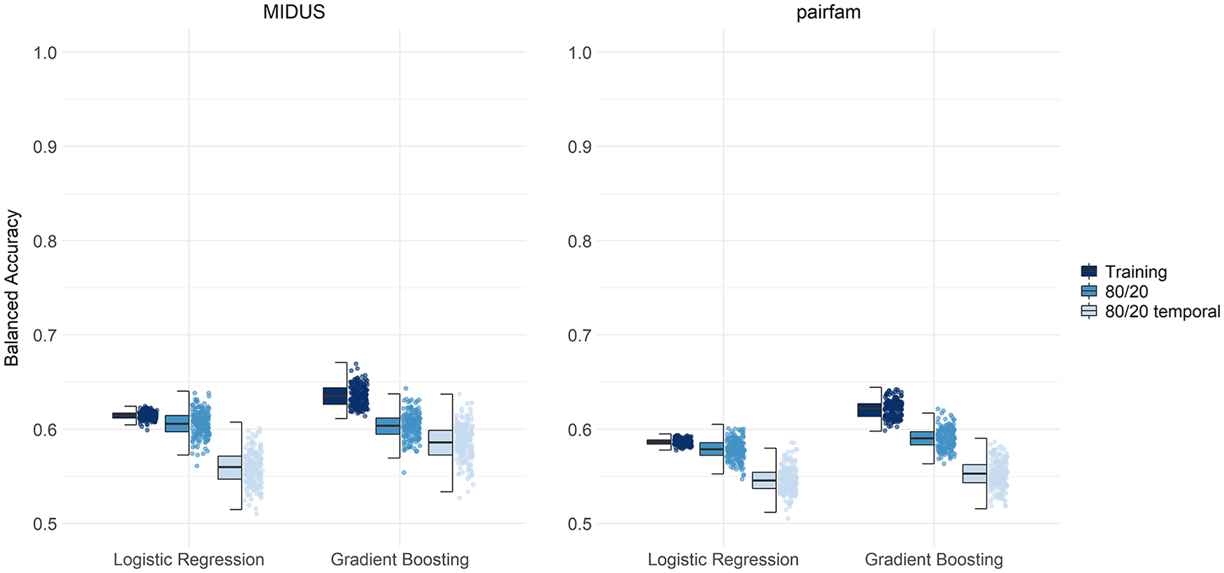
Balanced Accuracies for Predicting Attrition in MIDUS and pairfam. The boxplots represent the interquartile range, the solid line represents the median, and the whiskers 1.5 times the interquartile range. Balanced accuracy values of 200 randomly selected values are displayed as jittered distribution on the right with outliers as triangles.

Next, we focus on the disjoint temporal cross-validation. As to the question whether GBM outperforms logistic regression, the findings are mixed: Logistic regression yielded averaged balanced accuracies of .56 (MIDUS) and .55 (pairfam), and GBM achieved .59 (MIDUS) and .55 (pairfam) in the 80/20 temporal validation. Considering the much higher computational effort, the more complex (and ambiguous) model interpretation in GBM, and the mediocre overall balanced accuracies, the differences were—as in the traditional 80/20 validation approach—rather small and negligible.

To evaluate whether the respective models can be used for predicting attrition in future waves, the comparison of accuracies across both approaches are of particular interest. A decline in accuracies between the traditional 80/20 and the disjoint 80/20 approach was observed: For MIDUS, the averaged balanced accuracies of the 80/20 approach were higher (logistic regression: .61, GBM: .60) than those of the 80/20 temporal validation approach (.56 and .59, respectively). For pairfam, the nontemporal approach yielded higher averaged balanced accuracy values of .58 (logistic regression) and .59 (GBM) than the temporal validation with both .55. In summary, the already inaccurate prediction models lost further predictive accuracy when validated in a longitudinal framework.

The corresponding specificities and sensitivities for all models can be found as Supplemental Figures S3 und S4 in the OSF project (see at https://osf.io/usjr7/). For MIDUS, the averaged sensitivities were .53 (logistic regression) and .55 (GBM) and thus lower than the averaged specificities (.59 and .62, respectively). For pairfam, the averaged sensitivities were .55 (logistic regression) and .53 (GBM), hence nearly the same as the averaged specificities (.54 and .57, respectively). To conclude, these differences are rather small, but for MIDUS, the group of respondents could be detected slightly more accurately compared with the nonrespondents. These sensitivities translate to positive predictive values (i.e., the proportion of true nonrespondents of all participants who were flagged as nonrespondents) of .39 (logistic regression) and .41 (GBM) for MIDUS and .21 (logistic regression) and .22 (GBM) for pairfam.

Which Variables Predict Attrition?

For an overview of variable importances, we present the standardized regression coefficients of the logistic regression models averaged across all 1,000 iterations in Table 1. Overall, there was little consistency in regression coefficients across both surveys. For example, in MIDUS, the highest level of education was the predictor with the largest effect on attrition, whereas the level of education was not among the most important predictor variables in pairfam. Age had a negative effect on attrition in MIDUS (i.e., older participants were more likely to participate again) and a positive one in pairfam. In pairfam, the migration background was the second-most important variable, whereas in MIDUS migration background played no significant role in predicting attrition.

Table 1.

Averaged Standardized Coefficients of the Logistic Regression Models.

No.	MIDUS			pairfam
No.	Variable	M	SD	Variable	M	SD
1	Highest level of education	−.30	.02	Full–time employment	.24	.03
2	Age	−.27	.03	Migration background	.19	.02
3	Sex	−.25	.02	Homemaker	.15	.02
4	Instrumental activities of daily living	.19	.02	Number of household members	−.13	.02
5	Widow or widower	.16	.02	Age	.13	.03
6	Separated	.15	.02	Vocational training	.11	.01
7	Agreeableness	.15	.02	Self-employed	.11	.02
8	Conscientiousness	−.15	.02	Unemployed	.11	.02
9	Physical health, self-evaluated	−.14	.02
10	Divorced	.13	.02
11	Never been married	.12	.02
12	Current employment—Retired	−.12	.03
13	BMI	−.12	.02

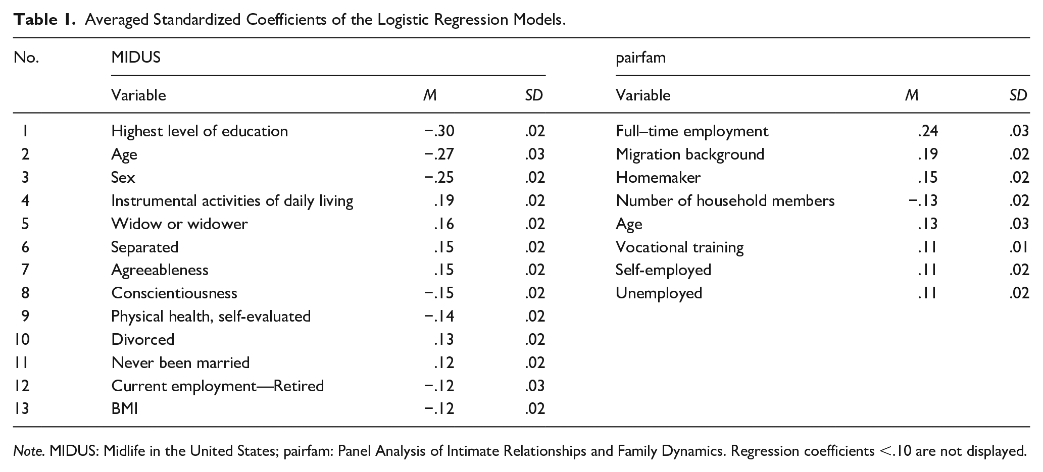
Note. MIDUS: Midlife in the United States; pairfam: Panel Analysis of Intimate Relationships and Family Dynamics. Regression coefficients <.10 are not displayed.

Discussion

High rates of systematic attrition can lead to biased results of studies using longitudinal data (Heffetz & Reeves, 2019; Little & Rubin, 2002). We argued that the optimal way to deal with attrition is to prevent it as best as possible, for example, with target-specific incentives. To achieve this goal, predicting attrition in future survey waves is more important than explaining possible underlying causal relationships of attrition. Thus, we focus on the prediction of attrition using machine learning algorithms in a longitudinal validation framework. The results of this study showed that the issue of attrition cannot be easily solved by applying more complex statistical models, that is, GBM did not outperform logistic regression analyses in predictive accuracy.

From a practical point of view, a central question is which strategy in dealing with attrition—target-specific incentives, equal distribution of incentives, over- or refreshment sampling—is most promising or cost-effective. The answer to this seemingly straightforward question depends on several parameters. For the following thought experiment, we focus on three of these parameters: (a) the overall available resources, (b) the percentage of participants who remained instead of dropping out, and (c) the positive predictive value of a prediction model. Let us assume that there is a budget of €20,000 available to implement retention measures to retain as much as possible of 1,000 (of 4,000) participants that are at risk of dropping out at a next survey wave. As a first strategy, one could prophylactically provide all 4,000 participants with incentives worth €5 such as sending thank you and birthday cards. With small investments per person, assuming a persuading effect of 5%, 50 of 1,000 at-risk participants could be converted.

A second approach could be to incentivize only those participants identified at risk of dropping out by a predictive model with €50 and assume that this will have the desired effect (staying active participants in the study) on 50% of them. The success of this second strategy depends on the predictive accuracy of the model. Within the budget of €20,000, using a perfect prediction model (positive predictive value = 1), it would be possible to persuade 200 participants to stay in the study (i.e., €20,000 / €50 = 400 participants, all of them get correctly flagged and funded, and half of them get convinced to stay). A model with a positive predictive value of .40 (as in our results for MIDUS) would still result in 80 participants (i.e., €20,000 / €50 = 400 participants, 40% of them get correctly flagged and funded, and half of them get convinced to stay). With a dropout rate of 25%, a model that is as accurate as random guessing would have a positive predictive value of .25 and result in 50 convinced participants (i.e., €20,000 / €50 = 400 participants, 25% of them get correctly flagged and funded, and half of them get convinced to stay). Thus, even small increments in positive predictive value translate into more successful retention of participants. However, there is no one-size-fits-all strategy that researchers must apply, rather the conditions of the individual longitudinal study have to be taken into account.

A third approach to deal with attrition could be to renounce the attempt of persuading participants and to sample new participants to replace all dropouts (refreshment). The cost of this approach depends on the number of waves a participant has been active (because the participants’ “value” accumulates across study waves) and on the resources needed for an assessment (e.g., online surveys are more economical than extensive examinations by medical professionals). However, retaining participants is always preferable over recruiting new ones (e.g., for analyzing intraindividual trajectories).

On the Generalizability of Prediction Models

The results concerning the variable importance were not generalizable across studies. In the introduction, we proposed four dimensions of generalizability: item sampling, person sampling, time sampling, and method sampling. First, different items and operationalizations of the same constructs (e.g., education and occupation) could have led to differences in variable importances. But also different cultural contexts could have a moderating effect. For example, although the participants’ migration background was defined in the same way in both studies, it could have a diverging effect due to different cultural and political implications in the United States and Germany (e.g., Berry et al., 2006). Second, the participants of MIDUS and pairfam already differed from each other at the respective baseline assessments. These different populations combined with the different topics of the panels also contributed to the nongeneralizability of effects: MIDUS is primarily concerned with midlife development of health and well-being, maybe leading to higher responding rates in older participants. In pairfam, younger nonsingle participants are more likely to participate again, which fits in with the fact that pairfam is a survey on partnership and family dynamics. Third, in MIDUS the survey waves are 9 years apart, whereas pairfam has annual survey waves and therefore places a higher burden on the resources of participants. However, regardless of the mechanisms underlying these differences, a model developed using MIDUS data cannot be used to predict attrition in pairfam and vice versa.

In addition to this nongeneralizability across items and persons, which also is true for cross-sectional studies, the nongeneralizability across measurement occasions is a specific that complicates matters in longitudinal studies. There is a very plausible explanation for this: If participants with certain characteristics drop out more likely, some of them will be no longer active participants at the next survey wave, altering the population for which nonresponse is to be predicted at a following survey wave. Either the same predictors also contribute to the prediction of nonresponse for the remaining individuals at future waves or their effects and importance also shift. The results of this study support the latter notion, that is, the reasons why people dropout change jointly with the participants. However, if one and the same model does not apply to or fit equally well for multiple survey waves, it is not useful for proactively planning survey retention strategies.

More Complex Models Are Not Better Suited to Predict Attrition

With respect to the last dimension of generalizability, the method sampling, the results are intriguing: The more complex data-driven models did not lead to substantial incremental in predictive accuracy in comparison with simple, logistic models. From this, one can conclude that the effects are mostly linear and that for reasons of parsimony a less complex model is preferable over computationally extensive and harder to interpret algorithms. The question arises, however, why other recent studies using machine learning algorithms to predict survey attrition reported relatively high predictive accuracies (e.g., Kern et al., 2019; Zinn & Gnambs, 2020). There are two reasons: First, in studies reporting higher accuracies, the previous response status was used as a predictor variable that, on one hand, was the most important predictor variable. However, on the other hand, this information is not available in longitudinal surveys without temporal nonrespondents (i.e., participants coming back at later study waves) as in this study. Second, it has been found that machine learning algorithms outperforming more simple models is often due to an insufficient distinction between training and testing samples (e.g., Jacobucci et al., 2021). In this study and in contrast to the traditional validation approach, we used a validation approach that also guarantees disjoint training and testing samples in a longitudinal context. Consequently, our predictive accuracies were lower.

To sum up, our rather strict approach at testing the accuracy of attrition models involving different survey occasions, two greatly differing longitudinal studies, and the comparison of a more basic modeling approach with a complex machine learning algorithm shed light on seldom asked, let alone solved problems within survey retention research. Since attrition models could not be generalized across studies and measurement occasions and their predictive accuracies were low in general, there is no clear answer to the question how to best tackle the issue of longitudinal attrition. However, under specific assumptions, even models with relatively low accuracies could be a useful tool for targeted incentives and for survey planning.

Footnotes

Declaration of Conflicting Interests

The author(s) declared no potential conflicts of interest with respect to the research, authorship, and/or publication of this article.

Funding

The author(s) received no financial support for the research, authorship, and/or publication of this article.

ORCID iDs

Kristin Jankowsky

Ulrich Schroeders

Supplemental Material

Supplemental material for this article is available online.

Notes

References

Behr

Giese

Teguim Kamdjou

H. D.

Theune

(2020). Early prediction of university dropouts—A Random Forest approach. Jahrbücher für Nationalökonomie und Statistik, 240(6), 743–789. https://doi.org/10.1515/jbnst-2019-0006

Beretta

Santaniello

(2016). Nearest neighbor imputation algorithms: A critical evaluation. BMC Medical Informatics and Decision Making, 16, Article 74. https://doi.org/10.1186/s12911-016-0318-z

Berry

J. W.

Phinney

J. S.

Sam

D. L.

Vedder

(2006). Immigrant youth: Acculturation, identity, and adaptation. Applied Psychology, 55(3), 303–332. https://doi.org/10.1111/j.1464-0597.2006.00256.x

Breiman

(2001). Random forests. Machine Learning, 45, 5–32. https://doi.org/10.1023/A:1010933404324

Brim

O. G.

Ryff

C. D.

Kessler

R. C.

(2004). The MIDUS national survey: An overview. In Brim

O. G.

Ryff

C. D.

Kessler

R. C.

(Eds.), How healthy are we? A national study of well-being at midlife (pp. 1–34). University of Chicago Press.

Deng

Hillygus

D. S.

Reiter

J. P.

Zheng

(2013). Handling attrition in longitudinal studies: The case for refreshment samples. Statistical Science, 28(2), 238–256. https://doi.org/10.1214/13-sts414

Dorsett

(2010). Adjusting for nonignorable sample attrition using survey substitutes identified by propensity score matching: An empirical investigation using labour market data. Journal of Official Statistics, 26(1), 105–125.

Dwyer

D. B.

Falkai

Koutsouleris

(2018). Machine learning approaches for clinical psychology and psychiatry. Annual Review of Clinical Psychology, 14(1), 91–118. https://doi.org/10.1146/annurev-clinpsy-032816-045037

Eisner

N. L.

Murray

A. L.

Eisner

Ribeaud

(2018). A practical guide to the analysis of nonresponse and attrition in longitudinal research using a real data example. International Journal of Behavioral Development, 43(1), 24–34. https://doi.org/10.1177/0165025418797004

10.

Enders

C. K.

(2010). Applied missing data analysis. Guilford Press.

11.

Friedman

J. H.

(2001). Greedy function approximation: A gradient boosting machine. Annals of Statistics, 29(5), 1189–1232. https://doi.org/10.1214/aos/1013203451

12.

Gelman

(2007). Struggles with survey weighting and regression modeling. Statistical Science, 22(2), 153–164. https://doi.org/10.1214/088342306000000691

13.

Greenwell

Boehmke

Cunnigham

., & GBM Developers. (2019). gbm: Generalized boosted regression models (Version 2.1.5) [Computer software]. https://CRAN.R-project.org/package=gbm

14.

Hardt

Herke

Leonhart

(2012). Auxiliary variables in multiple imputation in regression with missing X: A warning against including too many in small sample research. BMC Medical Research Methodology, 12(1), Article 184. https://doi.org/10.1186/1471-2288-12-184

15.

Heffetz

Reeves

D. B.

(2019). Difficulty of reaching respondents and nonresponse Bias: Evidence from large government surveys. Review of Economics and Statistics, 101(1), 176–191. https://doi.org/10.1162/rest_a_00748

16.

Huinink

Brüderl

Nauck

Walper

Castiglioni

Feldhaus

(2011). Panel Analysis of Intimate Relationships and Family Dynamics (pairfam): Conceptual Framework and Design. Zeitschrift für Familienforschung, 23(1), 77–101. https://madoc.bib.uni-mannheim.de/30017/

17.

Jacobsen

Ran

Liu

Chang

C.-C. H.

Ganguli

(2021). Predictors of attrition in a longitudinal population-based study of aging. International Psychogeriatrics, 33, 767–778. https://doi.org/10.1017/s1041610220000447

18.

Jacobucci

Littlefield

A. K.

Millner

A. J.

Kleiman

E. M.

Steinley

(2021). Evidence of inflated prediction performance: A commentary on machine learning and suicide research. Clinical Psychological Science, 9(1), 129–134. https://doi.org/10.1177/2167702620954216

19.

Jeličić

Phelps

Lerner

R. M.

(2009). Use of missing data methods in longitudinal studies: The persistence of bad practices in developmental psychology. Developmental Psychology, 45(4), 1195–1199. https://doi.org/10.1037/a0015665

20.

Kern

Weiss

Kolb

J.-P.

(2019). A longitudinal framework for predicting nonresponse in panel surveys. arXiv: 1909.13361

21.

Kleinke

Reinecke

Daniel

Spiess

(2020). Applied multiple imputation: Advantages, pitfalls, new developments and applications in R. Springer.

22.

Kuhn

(2008). Building predictive models in r using the caret package. Journal of Statistical Software, 28(5), 1–26. https://doi.org/10.18637/jss.v028.i05

23.

Little

R. J. A.

Rubin

D. B.

(2002). Statistical analysis with missing data (2nd ed.). Wiley.

24.

Lugtig

(2014). Panel attrition: Separating stayers, fast attriters, gradual attriters, and lurkers. Sociological Methods & Research, 43(4), 699–723. https://doi.org/10.1177/0049124113520305

25.

Lynn

(2017). From standardised to targeted survey procedures for tackling nonresponse and attrition. Survey Research Methods, 11(1), 93–103. https://doi.org/10.18148/srm/2017.v11i1.6734

26.

Mustillo

Kwon

(2014). Auxiliary variables in multiple imputation when data are missing not at random. The Journal of Mathematical Sociology, 39(2), 73–91. https://doi.org/10.1080/0022250x.2013.877898

27.

Nicholson

J. S.

Deboeck

P. R.

Howard

(2017). Attrition in developmental psychology: A review of modern missing data reporting and practices. International Journal of Behavioral Development, 41(1), 143–153. https://doi.org/10.1177/0165025415618275

28.

Pforr

Blohm

Blom

A. G.

Erdel

Felderer

Fräßdorf

Hajek

Helmschrott

Kleinert

Koch

Kreiger

Kroh

Saßenroth

Schmiedeberg

Trüdinger

E. -M.

Rammstedt

(2015). Are incentive effects on response rates and nonresponse bias in large-scale, face-to-face surveys generalizable to Germany? Evidence from ten experiments. Public Opinion Quarterly, 79(3), 740–768. https://doi.org/10.1093/poq/nfv014

29.

Rackoff

G. N.

Newman

M. G.

(2020). Reduced positive affect on days with stress exposure predicts depression, anxiety disorders, and low trait positive affect 7 years later. Journal of Abnormal Psychology, 129(8), 799–809. https://doi.org/10.1037/abn0000639

30.

Radler

B. T.

Ryff

C. D.

(2010). Who participates? Accounting for longitudinal retention in the MIDUS national study of health and well-being. Journal of Aging and Health, 22(3), 307–331. https://doi.org/10.1177/0898264309358617

31.

Rocca

Yarkoni

(2020, November 12). Putting psychology to the test: Rethinking model evaluation through benchmarking and prediction. https://doi.org/10.31234/osf.io/e437b

32.

Schafer

J. L.

Graham

J. W.

(2002). Missing data: Our view of the state of the art. Psychological Methods, 7(2), 147–177. https://doi.org/10.1037//1082-989X.7.2.147

33.

Schmidt

Woll

(2017). Longitudinal drop-out and weighting against its bias. BMC Medical Research Methodology, 17, Article 164. https://doi.org/10.1186/s12874-017-0446-x

34.

Schoeni

R. F.

Stafford

Mcgonagle

K. A.

Andreski

(2012). Response rates in national panel surveys. The ANNALS of the American Academy of Political and Social Science, 645(1), 60–87. https://doi.org/10.1177/0002716212456363

35.

Schroeders

Schmidt

Gnambs

(2022). Detecting careless responding in survey data using stochastic gradient boosting. Educational and Psychological Measurement, 82(1), 29–56. https://doi.org/10.1177/00131644211004708

36.

Seaman

S. R.

White

I. R.

(2013). Review of inverse probability weighting for dealing with missing data. Statistical Methods in Medical Research, 22(3), 278–295. https://doi.org/10.1177/0962280210395740

37.

Shmueli

(2010). To explain or to predict? Statistical Science, 25(3), 289–310. https://projecteuclid.org/euclid.ss/1294167961

38.

Van Buuren

. (2018). Flexible imputation of missing data (2nd ed.). CRC Press.

39.

Voelkle

M. C.

Brose

Schmiedek

Lindenberger

(2014). Toward a unified framework for the study of between-person and within-person structures: Building a bridge between two research paradigms. Multivariate Behavioral Research, 49(3), 193–213. https://doi.org/10.1080/00273171.2014.889593

40.

Yarkoni

Westfall

(2017). Choosing prediction over explanation in psychology: Lessons from machine learning. Perspectives on Psychological Science, 12(6), 1100–1122. https://doi.org/10.1177/1745691617693393

41.

Young

A. F.

Powers

J. R.

Bell

S. L.

(2006). Attrition in longitudinal studies: Who do you lose? Australian and New Zealand Journal of Public Health, 30(4), 353–361. https://doi.org/10.1111/j.1467-842x.2006.tb00849.x

42.

Zinn

Gnambs

(2020). Analyzing nonresponse in longitudinal surveys using Bayesian Additive Regression Trees: A nonparametric event history analysis. Social Science Computer Review. Advance online publication. https://doi.org/10.1177/0894439320928242

43.

Zou

Hastie

(2005). Regularization and variable selection via the elastic net. Journal of the Royal Statistical Society: Series B (Statistical Methodology), 67(2), 301–320. https://doi.org/10.1111/j.1467-9868.2005.00503.x

Validation and generalizability of machine learning prediction models on attrition in longitudinal studies

Abstract

Keywords

Strategies in Dealing With Panel Attrition

Drawbacks of Common Approaches to Analyzing Panel Attrition

Predicting Panel Attrition Using Machine Learning

The Present Study

Method

Sample and Design

MIDUS

Pairfam

Measures

Statistical Analyses

Results

Which Variables Predict Attrition?

Discussion

On the Generalizability of Prediction Models

More Complex Models Are Not Better Suited to Predict Attrition

Footnotes

Declaration of Conflicting Interests

Funding

ORCID iDs

Supplemental Material

Notes

References