Sage Journals: Discover world-class research

Abstract

The analysis of cross-lagged relationships is a popular approach in prevention research to explore the dynamics between constructs over time. However, a limitation of commonly used cross-lagged models is the requirement of equally spaced measurement occasions that prevents the usage of flexible longitudinal designs and complicates cross-study comparisons. Continuous-time modeling overcomes these limitations. In this article, we illustrate the use of continuous-time models using Bayesian and frequentist approaches to model estimation. As an empirical example, we study the dynamic interplay of physical activity and health, a classic research topic in prevention science, using data from the “Midlife in the United States (MIDUS 2): Daily Stress Project, 2004–2009.” To help prevention researchers in adopting the approach, we provide annotated R scripts and a simulated data set based on the results from analyzing the MIDUS 2 data.

Keywords

Continuous-time models longitudinal data autoregressive models cross-lagged models

In prevention research, many studies have been concerned with the bidirectional, dynamic interplay of psychological, medical, and health-related variables and constructs. For instance, physical activity (PA) was related to academic performance (Aaltonen et al., 2016), executive functioning (Farina, Tabet, & Rusted, 2016), depression (Lindwall, Larsman, & Hagger, 2011; Stavrakakis, de Jonge, Ormel, & Oldehinkel, 2012), fear-avoidance beliefs (Leonhardt et al., 2009), allostatic load (Read & Grundy, 2014), and habit (van Bree et al., 2017); health was related to social activities (Kim & Yoon, 2017) and depression (Kim, Noh, Park, & Kwon, 2014). The argumentation in such studies often starts with the observation that two variables are associated, but that the directionality of the association is unclear. Therefore, longitudinal designs are chosen to predict values of a variable from previous values of another variable. In fact, temporal priority is usually considered one necessary condition for causality (e.g., Chambliss & Schutt, 2016). One common statistical method for modeling the interplay of repeatedly measured variables is cross-lagged panel analysis (e.g., Kearney, 2017; Selig & Little, 2012), sometimes also referred to as linear panel models (Greenberg & Kessler, 1982), causal models (Bentler, 1980), or autoregressive cross-lagged models (Bollen & Curran, 2006). The primary objective of cross-lagged analysis is “to examine the stability and relationships between variables over time to better understand how variables influence each other over time” (Kearney, 2017, p. 312). The amount of stability in a construct is described by an autoregressive effect, that is, the regression coefficient when a variable is regressed on itself at a previous point in time. In the social sciences, smaller autoregressive coefficients (closer to zero) are often interpreted as indicating less stability, whereas larger autoregressive coefficients indicate more stability (Kearney, 2017). The cross-lagged effects represent the effect of a previous state of a variable on another variable controlled for the prior level of the variable predicted. This control strategy allows one to rule out the possibility that a cross-lagged effect is only due to the fact that the two variables are correlated at the previous time point (Selig & Little, 2012) and is also necessary to minimize bias in the estimation of cross-lagged effects (Cole & Maxwell, 2003; Gollob & Reichardt, 1987). Although several limitations and drawbacks of cross-lagged models have been at the center of discussion (cf. Kearney, 2017; Selig & Little, 2012), there clearly “is a place for the use of the panel model in developmental research” (Selig & Little, 2012, p. 269), because they can help to better understand the longitudinal relations between variables.

One major issue that needs consideration, however, is the role of time and the implications of how time is incorporated (see, e.g., Voelkle, Gische, Driver, & Lindenberger, 2018). In crossed-lagged models, the autoregressive and cross-lagged effects depend on the chosen time interval length between discrete measurement occasions. In practice, this often implies several disadvantages: (1) Constant interval lengths between measurement occasions within a study need to be assured. This prevents researchers from modeling data from flexible longitudinal designs that are, for instance, heavily used in experience sampling, ambulatory assessment, and ecological momentary assessment approaches. (2) Cross-study comparisons are complicated because identical effects may appear different if different time intervals are being used across studies, whereas different effects may incorrectly appear similar (Voelkle, Oud, Davidov, & Schmidt, 2012). (3) The researcher faces the challenging task of choosing exactly the right time interval at which an effect occurs. To overcome these shortcomings, continuous-time models have been proposed (cf. van Montfort, Oud, & Voelkle, 2018). As we demonstrate in the next section, continuous-time models (1) permit the analysis of data from flexible longitudinal designs with differing time intervals between and within individuals, (2) facilitate cross-study comparisons, and (3) allow for exploring the unfolding of effects across time.

Continuous-time models have a long history (Bergstrom, 1988), and the relationship between discrete-time and continuous-time models has been discussed by many authors (for a recent overview of continuous-time models in the behavioral and related sciences, see van Montfort et al., 2018). Theoretically, we can distinguish between processes that occur only at discrete time points and processes that exist continuously, but are only observed at discrete time points. Arguably, most processes in the behavioral and related sciences are of the latter kind. Mood, health, and cognitive functioning are all constructs that exist continuously within a person, but are only observed at selected time points.

If the discrete-time model is the true data-generating model for the processes, then only values at specific moments in time (i.e., discrete occasions) exist. Their serial dependency is described by the autoregressive effects and the cross-lagged effects. In contrast, a continuous-time model assumes the continuous existence of the process. Theoretically, it would be possible to measure this process at any arbitrary point in time. In practice, however, there exist only few discrete measurement occasions, and the continuous-time model tries to identify the continuous-time process that has led to these discrete measures.

Purpose and Scope

We describe and illustrate continuous-time models using an empirical example with a prototypical research question from prevention research: Are people who engage in sports/physical activities more healthy or do healthy people engage in more sports/physical activities?

This question was, for instance, raised by Becker (2011) and is of gerontological, medical-sociological, economic, sport-scientific, and public health-related relevance. Of course, this general research question can and needs to be broken down into concrete operationalizations, time frames of effects, and targeted populations. For instance, a systematic review by Reiner, Niermann, Jekauc, and Woll (2013) summarizes long-term health benefits of PA for adults within the age range of 18–85 years. For school-aged children and youth, a systematic review was conducted by Janssen and LeBlanc (2010), for adolescents by Granger et al. (2017), and for 0- to 4-year-old children by Timmons et al. (2012). Results from studies investigating short-term relationships between PA and health have been systematically reviewed by Bravata et al. (2007). Systematic reviews that concern the relationship of PA and pain can, for instance, be found in the publications by Sitthipornvorakul, Janwantanakul, Purepong, Pensri, and van der Beek (2011) and Geneen et al. (2017).

Results across studies, populations, and operationalizations seem to be inconsistent. For example, Sitthipornvorakul et al. (2011) report that “[c]onflicting evidence was found for the association between physical activity and low back pain in both general population and school children” (p. 683), whereas “[s]trong evidence was found for no association between physical activity and neck pain among school children” (p. 683). Geneen et al. (2017) report inconsistent results as well but state that at least PA appears to not cause harm. Granger et al. (2017) also report that “there is conflicting evidence regarding the relationship between PA levels and self-reported health status” (p. 100) for adolescents. In contrast, “[n]o serious inconsistency in any of the studies reviewed” (Timmons et al., 2012, p. 773) were found when investigating the relationship between PA and health in the early years. For the population of toddlers, there was “moderate-quality evidence to suggest that increased or higher PA was positively associated with bone and skeletal health” (Timmons et al., 2012, p. 773). In a similar vein, Janssen and LeBlanc (2010) state that the findings of their systematic review “confirm that physical activity is associated with numerous health benefits in school-aged children and youth” (p. 13). Likewise, Reiner et al. (2013) conclude that “physical activity appears to have a positive long-term influence on all selected diseases” (p. 1). In summary, there is no general consensus concerning the relationship between PA and health, and their dynamic interplay (i.e., the question whether PA affects health and/or health affects PA) is unclear.

The bidirectional nature of such a research question clearly calls for models in which both effects (i.e., PA on health as well as health on PA) are included, like bivariate continuous-time models. We use longitudinal data from the “Midlife in the United States (MIDUS 2): Daily Stress Project, 2004–2009” (Ryff & Almeida, 2017) and the R package ctsem (Driver, Oud, & Voelkle, 2017). We provide ctsem syntax for frequentist and Bayesian model estimation to illustrate the flexibility of the approach and to help other researchers in adopting the approach within their preferred modeling framework.

The article is organized as follows: We start by (1) describing multivariate continuous-time models for normally distributed manifest variables. Next, we (2) use a bivariate continuous-time model on empirical data for illustration purposes and finally (3) conclude with a discussion of our work.

Multivariate Continuous-Time Models

In this section, we briefly describe multivariate continuous-time models using matrix algebra formulations. Readers who are less interested in technicalities but primarily interested in the application of continuous-time models may skip this section and proceed directly to the empirical example. Researchers who are interested in a stepwise introduction to the mathematical-technical background of the approach are referred to Voelkle et al. (2012). For details on Bayesian hierarchical continuous-time models, see Driver and Voelkle (2018) and Hecht, Hardt, Driver, and Voelkle (2019).

In longitudinal designs with unequally spaced measurement occasions, there are responses of j = 1,…, J persons at several points in time, t_jp , with p = 1,…, P_j being a running index that denotes the discrete measurement occasion and P_j being the person-specific number of measurement occasions (see Hecht, Hardt, et al., 2019, for details and illustrations). The manifest responses, θ_jpf, of person j at measurement occasion p on variable f = 1,…, F (with F being the total number of variables or “processes”) are stacked into the column vector θ _jp.

The continuous-time model is given by:

d θ_{j} (t) = (A θ_{j} (t) + b + b_{j}) d t + G d W_{j} (t)

with

Q = G G'

where A is the square drift matrix of order F containing the continuous-time auto-effects on the main diagonal and cross-effects on the off-diagonals; Q is the symmetric diffusion covariance matrix of order F containing the diffusion variances on the main diagonal and the diffusion covariances on the off-diagonals; G is the Cholesky factor of the diffusion covariance matrix Q and scales the white noise represented by $d W_{j} (t)$ ; b is a column vector with F continuous-time intercepts; and $b_{j}$ is a column vector with person-specific deviations from the continuous-time intercepts (for details, see Driver & Voelkle, 2018; Oud & Delsing, 2010; Voelkle et al., 2012). Solving this equation for a given starting point and a time interval leads to the discrete-time model:

θ_{j p} = A_{Δ_{j (p - 1)}}^{*} θ_{j (p - 1)} + b_{Δ_{j (p - 1)}}^{*} + b_{j Δ_{j (p - 1)}}^{*} + ω_{j (p - 1)}

ω_{j (p - 1)} \sim N (0, Q_{Δ_{j (p - 1)}}^{*})

for p ≥ 2, where $A_{Δ_{j (p - 1)}}^{*}$ is the square autoregression matrix of order F containing the autoregressive effects on the main diagonal and the cross-lagged effects on the off-diagonals; $Q_{Δ_{j (p - 1)}}^{*}$ is the symmetric process error covariance matrix of order F containing the process error variances on the main diagonal and the process error covariances on the off-diagonals; $b_{Δ_{j (p - 1)}}^{*}$ is a column vector containing F discrete-time intercepts; and $b_{j Δ_{j (p - 1)}}^{*}$ is a column vector containing person-specific deviations from the discrete-time intercepts. These discrete-time parameters all depend on person-specific and occasion-specific interval lengths Δ _j ₍ _p ₋ ₁₎ = t_jp − t_j ₍ _p ₋ ₁₎ and can be calculated from the continuous-time parameters, equations (5) to (11) in the Appendix (for examples and illustrations, see Hecht, Hardt, et al., 2019). In Table 1, we provide an overview of possible terms to distinguish corresponding discrete-time and continuous-time parameters.

Table 1.

Discrete-Time Versus Continuous-Time Parameter Labels.

Discrete time		Continuous time
Parameter	Label	Parameter	Label
$A_{Δ}^{*}$	Autoregression matrix	$A$	Drift matrix
$A_{Δ}^{*}$ [k, k]	Autoregressive effect	$A$ [k, k]	Auto-effect
$A_{Δ}^{*}$ [k, l]	Cross-lagged effect	$A$ [k, l]	Cross-effect
$Q_{Δ}^{*}$	Process error^a matrix	$Q$	Diffusion covariance matrix
$Q_{Δ}^{*}$ [k, k]	Process error^a variance	$Q$ [k, k]	Diffusion variance
$Q_{Δ}^{*}$ [k, l]	Process error^a covariance	$Q$ [k, l]	Diffusion covariance
$b_{Δ}^{*}$	Dt intercepts	$b$	Ct intercepts
$Σ_{bΔ}^{*}$	Dt intercepts covariance matrix	$Σ_{b}$	Ct intercepts covariance matrix
$Σ_{bΔ}^{*}$ [k, k]	Dt intercepts variance	$Σ_{b}$ [k, k]	Ct intercepts variance
$Σ_{bΔ}^{*}$ [k, l]	Dt intercepts covariance	$Σ_{b}$ [k, l]	Ct intercepts covariance

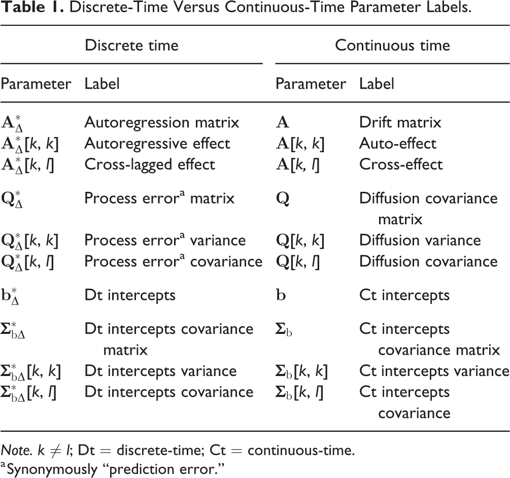
Note. k ≠ l; Dt = discrete-time; Ct = continuous-time.

^a Synonymously “prediction error.”

In autoregressive models, the prediction from a previous measurement occasion is lacking for the first measurement occasion (p = 1). Options for conceptualizing, estimating, and imposing stationarity constraints on parameters related with modeling the first measurement occasion can be found in the work of Driver et al. (2017) and Driver and Voelkle (2018).

Empirical Example

Data

We used data from the “Midlife in the United States (MIDUS 2): Daily Stress Project, 2004–2009” (Ryff & Almeida, 2017), namely variables B2DA4AH/B2DA4AM (PA in hours/minutes) and B2DSYMAV (average symptom severity [SS], 1 = very mild, 10 = very severe). The former two variables were combined into one variable that indicates PA in hours since the interviewer last spoke with the respondent, that is, the amount of PA roughly in the last 24 hr (Inter-university Consortium for Political and Social Research [ICPSR] user support, personal communication, January 9, 2019). The original data set contains data from 2,022 study participants who were each assessed on eight consecutive days.

Treatment of Extreme Cases and Missing Values

The data from 372 persons were deleted, because they had a value of zero for all PA measurements and thus do not belong to the population of interest (i.e., persons who engage in PA). For the remaining 1,650 persons, there are no missing values on the variable SS, that is, all 1,650 × 8 = 13,200 values are observed. On the variable PA, 940 values (7.1%) are missing with zero to seven (M = 0.57, SD = 1.19) missing values per person. Missing values are dealt with by full information maximum likelihood (FIML) estimation, which is also the default setting in ctsem (Oud & Voelkle, 2014; Voelkle & Oud, 2013). In principle, FIML may be complemented and/or replaced by other approaches to deal with missing values such as multiple imputation. However, future research is necessary to evaluate such alternatives. Further, the option to use auxiliary variables (e.g., Collins, Schafer, & Kam, 2001) is not yet implemented in ctsem.

Descriptive Statistics

The person means (across the eight measurement occasions) ranged from 0.01 hr to 10.50 hr (M = 0.83, SD = 1.01) for PA and from 0.98 to 8.01 (M = 2.53, SD = 1.31) for SS. The within-person standard deviations ranged from 0 hr to 5.50 hr (M = 0.85, SD = 0.83) for PA and from 0 to 4.39 (M = 1.14, SD = 0.73) for SS. The age of persons in our sample ranged from 33 years to 83 years (M = 56.28, SD = 12.17) and 55.9% were female and 44.1% male.

Model

We estimated the multivariate continuous-time model described above for F = 2 variables, that is, PA and SS, assuming that the processes are stationary. Thus, there are 12 free model parameters as defined above: drift matrix with auto-effects and cross-effects: $A = [\begin{matrix} a_{PA} & a_{SS \to PA} \\ a_{PA \to SS} & a_{SS} \end{matrix}]$ , diffusion covariance matrix: $Q = [\begin{matrix} σ_{PA}^{2} & σ_{PA \leftrightarrow SS} \\ σ_{PA \leftrightarrow SS} & σ_{SS}^{2} \end{matrix}]$ , continuous-time intercepts: $b = [\begin{matrix} b_{PA} \\ b_{SS} \end{matrix}]$ , and covariance matrix of continuous-time intercepts: $Σ_{b} = [\begin{matrix} σ_{b_{PA}}^{2} & σ_{b_{PA \leftrightarrow SS}} \\ σ_{b_{PA \leftrightarrow SS}} & σ_{b_{SS}}^{2} \end{matrix}]$ .

Analysis

We ran the continuous-time model using R 3.5.2 (R Core Team, 2018) and the R package ctsem (Driver, Oud, & Voelkle, 2018), which offers frequentist estimation of continuous-time models by interfacing to OpenMx (Neale et al., 2016) and Bayesian estimation by interfacing to the Stan software (Carpenter et al., 2017). To illustrate the flexibility of the approach and to help other researchers in adopting it within their preferred modeling framework, we report the results of both and provide the scripts for both approaches in the Online Supplemental Material. In particular, Bayesian models are gaining in popularity in many disciplines and are used for many different reasons, for instance, to include previous knowledge, to estimate otherwise intractable models, to model uncertainty (van de Schoot, Winter, Ryan, Zondervan-Zwijnenburg, & Depaoli, 2017), and to stabilize parameter estimates (e.g., Zitzmann, 2018). However, often an obstacle is the long run time that might prevent users from using Bayesian estimation. Therefore, users of the R package ctsem can decide whether the advantages of the Bayesian estimation (e.g., the possibility to include prior information) justifies the long model run time. As shown below, for weakly informative priors, the Bayesian and frequentist estimation come to roughly the same results. Thus, the much faster frequentist estimation may be preferred in the case of weak prior information (and given that the model is implementable in the frequentist framework).

The function ctFit() of the R package ctsem provides frequentist estimation using maximum likelihood, whereas Bayesian estimation is implemented by the function ctStanFit(). The complete syntax to run the model in both estimation frameworks on a simulated data set based on our results is provided in the Online Supplemental Material. For the frequentist model, we used the OpenMx default optimizer CSOLNP and for the Bayesian model the default burnin (50% of the chain), the default aggregation statistic (mean of the chain), and the default priors (see Driver & Voelkle, 2018), the latter being “weakly informative for typical conditions in the social sciences” (Hecht, Hardt, et al., 2019, p. 9). We ran the Bayesian model with one chain and 16,000 iterations. As a convergence statistic, we report the potential scale reduction factor $\hat{R}$ (Gelman & Rubin, 1992) and as a precision statistic the effective sample size (for a discussion of both, see, e.g., Zitzmann & Hecht, 2019). Run time and RAM usage of the frequentist estimation were barely noticeable, whereas the Bayesian estimation needed approximately 2.64 GB RAM and 2 days and 20 hr run time¹ on one Intel Xeon Gold 5120 (2.20 GHz) CPU of a 64-bit Linux Debian 9 “Stretch” computer (kernel version 4.9.0-8-amd64).

Results

Table 2 presents the results of the continuous-time model estimated with the frequentist and Bayesian estimation methods. In the Bayesian model, convergence ( $\hat{R}$ ) and precision (N _eff) were very satisfactory for all parameters. Results between both estimation methods differ just slightly. For this reason, we focus on the parameter estimates from the frequentist approach in the following. The continuous-time parameters describe the underlying process “independent” of the length of the time intervals between discrete measurement occasions and can be used to derive corresponding discrete-time parameters for any arbitrary interval length. The technical details of this computation are provided in equations (5) to (11) in the Appendix. Figure 1 shows the dependency of derived discrete-time parameters on time interval length for our model. Clearly, all model-implied discrete-time parameters vary depending on the time interval length. The auto-effects decrease with increasing interval length. This is plausible as a value is less predictive for the consecutive value the more time passes. The cross-lagged effects follow an inverse U-shape in our example, with the maxima for an interval length of roughly half a day. The process error variation, the discrete-time intercept variation, and the discrete-time intercepts increase with increasing interval length and converge to their asymptotic long-range values (displayed as solid horizontal lines).

Figure 1.

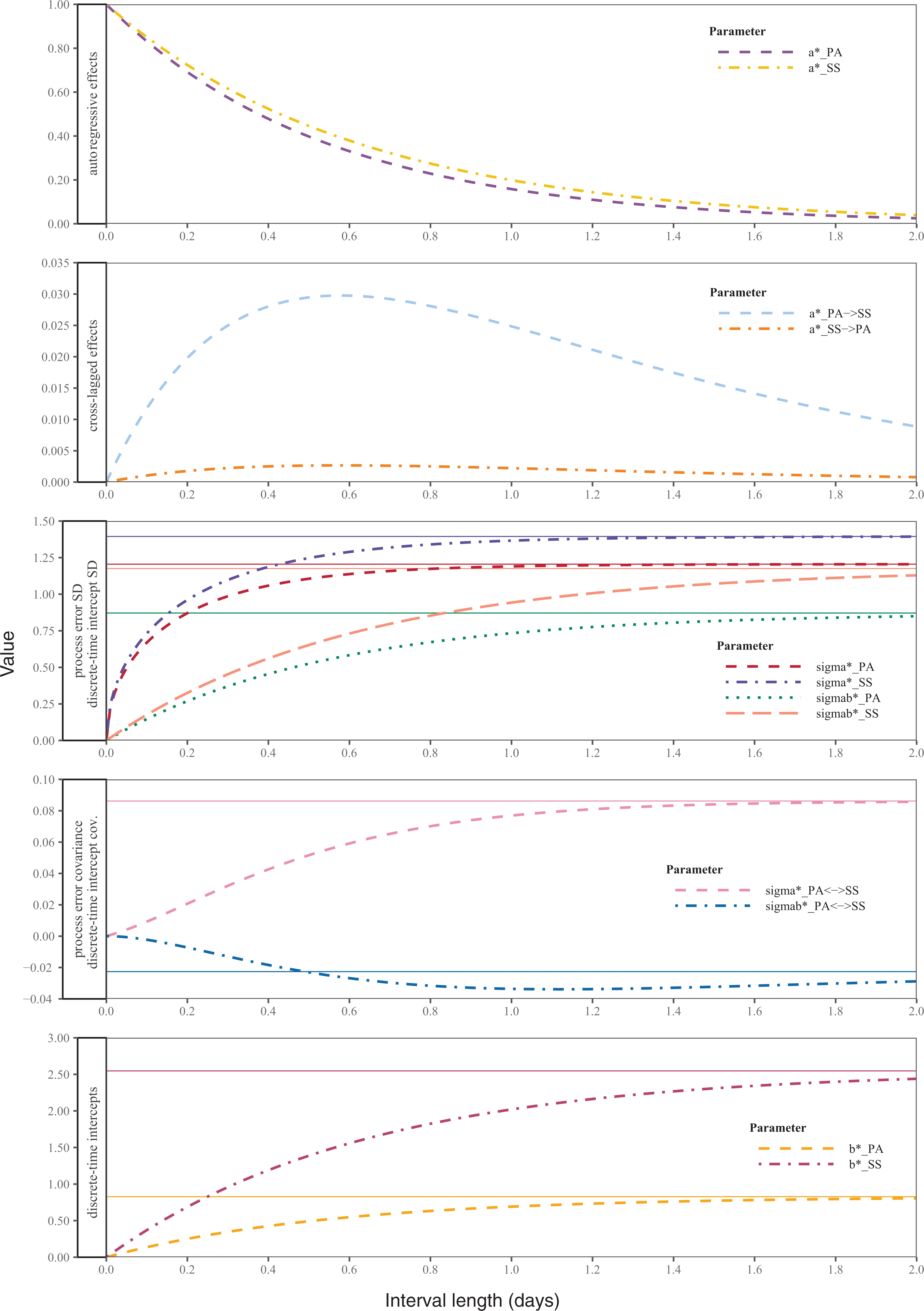
Model-Implied Derived Discrete-Time Parameters Depending on Time Interval Length. Note. Solid horizontal lines represent asymptotic long-range parameter values.

Table 2.

Results of the Frequentist and Bayesian Continuous-Time Model for Physical Activity and Symptom Severity (MIDUS 2 data).

		Frequentist estimation					Bayesian estimation
Parameter name	Parameter	Est.	SE	p	95% CI		Est.	95% BCI		$\hat{R}$	N _eff
Parameter name	Parameter	Est.	SE	p	LL	UL	Est.	LL	UL	$\hat{R}$	N _eff
Auto-effect	$a_{PA}$	−1.845	.078	<.001	−1.999	−1.691	−1.862	−2.032	−1.713	1.000	4,465
Auto-effect	$a_{SS}$	−1.617	.059	<.001	−1.733	−1.501	−1.627	−1.751	−1.513	1.000	4,095
Cross-effect	$a_{PA \to SS}$	0.140	.072	.053	−0.002	0.282	0.141	−0.002	0.284	1.000	4,382
Cross-effect	$a_{SS \to PA}$	0.013	.055	.818	−0.095	0.120	0.014	−0.092	0.120	1.000	2,626
Diffusion SD	$σ_{PA}$	2.315	.044	<.001	2.228	2.402	2.324	2.240	2.418	1.000	6,096
Diffusion SD	$σ_{SS}$	2.503	.040	<.001	2.425	2.581	2.510	2.433	2.592	1.000	5,451
Diffusion correlation	$r_{PA \leftrightarrow SS}$	0.012	.025	.627	−0.037	0.061	0.010	−0.031	0.055	1.000	5,046
Ct intercept	$b_{PA}$	1.496	.154	<.001	1.193	1.798	1.505	1.213	1.811	1.000	2,904
Ct intercept	$b_{SS}$	4.002	.162	<.001	3.685	4.320	4.028	3.712	4.376	1.000	4,179
Ct intercept SD	$σ_{b_{PA}}$	1.608	.084	<.001	1.444	1.772	1.628	1.467	1.810	1.000	2,371
Ct intercept SD	$σ_{b_{SS}}$	1.907	.087	<.001	1.736	2.078	1.923	1.761	2.107	1.000	2,474
Ct intercept correlation	$r_{b_{PA \leftrightarrow SS}}$	−0.095	.069	.170	−0.231	0.041	−0.095	−0.230	0.040	1.000	2,068

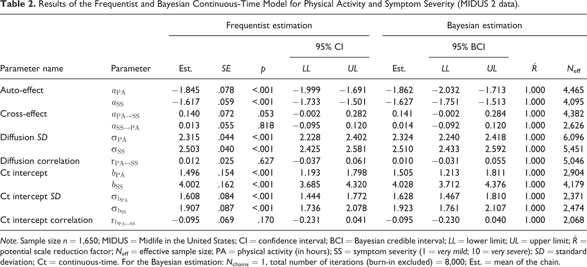
Note. Sample size n = 1,650; MIDUS = Midlife in the United States; CI = confidence interval; BCI = Bayesian credible interval; LL = lower limit; UL = upper limit; $\hat{R}$ = potential scale reduction factor; N _eff = effective sample size; PA = physical activity (in hours); SS = symptom severity (1 = very mild; 10 = very severe); SD = standard deviation; Ct = continuous-time. For the Bayesian estimation: N _chains = 1, total number of iterations (burn-in excluded) = 8,000; Est. = mean of the chain.

Figure 1 illustrates some key advantages of continuous-time models over discrete-time models. As can be seen, the discrete-time parameters differ depending on the length of the time interval between measurements. Thus, studies in which discrete-time cross-lagged models based on different time intervals were used would come to different results and conclusions, whereas this problem is resolved in continuous-time models. Further, discrete-time models rely on equal-interval nonindividualized spacings of measurement occasions and may perform poorly when this design feature is not given (De Haan-Rietdijk, Voelkle, Keijsers, & Hamaker, 2017; Hecht, Hardt, et al., 2019).

However, in contrast to discrete-time parameters, the parameter estimates of the continuous-time model (reported in Table 2) lack an intuitive interpretation. For reasons of interpretation, it is thus useful to transform them back into well interpretable discrete-time parameters. Here, the advantage of continuous-time models come into play again: we are not bound to the interval length used for data collection, but can choose any time interval of interest. For instance, for a discrete-time model describing day-to-day effects, we calculate the discrete-time parameters for the interval length Δ = 1 day using equations (5) to (11) in the Appendix. The autoregression matrix for this time interval is then:

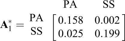
A_{1}^{*} = \begin{matrix} PA \\ SS \end{matrix} \begin{matrix} PA & SS \\ [\begin{matrix} 0.158 & 0.002 \\ 0.025 & 0.199 \end{matrix}] \end{matrix}

We see that there are low autoregressive effects for both processes. That means that PA on one day has only a weak effect on PA the following day. The same holds for SS: there is only a small effect of SS on one day on SS the next day. The cross-lagged effects are essentially zero and nonsignificant; thus, there is no relevant impact from one variable on the other.

The long-range within-person process variation characterizes the uncertainty about process states for a time interval approaching infinity. Likewise, the long-range process means and their between-person variation describe the mean levels and individual differences in mean levels for a time interval approaching infinity. From these parameters (see Table 3), we can compute the fraction of between-person variation to total variation, which is often called “intra-class correlation,” for both processes:

Table 3.

Long-Range Parameters.

Parameter name	Parameter	Value
Long-range process SD	$σ_{\infty_{PA}}^{*}$	1.205
Long-range process SD	$σ_{\infty_{SS}}^{*}$	1.395
Long-range processes correlation	$r_{\infty_{PA \leftrightarrow SS}}^{*}$	0.051
Long-range mean	$μ_{θ \infty_{PA}}^{*}$	0.828
Long-range mean	$μ_{θ \infty_{SS}}^{*}$	2.547
Long-range means SD	$σ_{μ_{θ \infty_{PA}}}^{*}$	0.871
Long-range means SD	$σ_{μ_{θ \infty_{SS}}}^{*}$	1.175
Long-range means correlation	$r_{μ_{θ \infty_{PA \leftrightarrow SS}}}^{*}$	−0.022

Note. SD = standard deviation. For the calculation of long-range parameters, results from the frequentist model and equations (13), (14), and (16) from the Appendix were used.

{ICC}_{PA} = \frac{σ_{μ_{θ \infty_{PA}}}^{2^{*}}}{σ_{μ_{θ \infty_{PA}}}^{2^{*}} + σ_{\infty_{PA}}^{2^{*}}} = \frac{{0.871}^{2}}{{0.871}^{2} + {1.205}^{2}} = 0.343

{ICC}_{SS} = \frac{σ_{μ_{θ \infty_{SS}}}^{2^{*}}}{σ_{μ_{θ \infty_{SS}}}^{2^{*}} + σ_{\infty_{SS}}^{2^{*}}} = \frac{{1.175}^{2}}{{1.175}^{2} + {1.395}^{2}} = 0.415

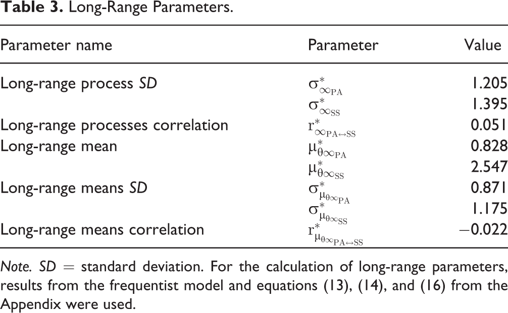
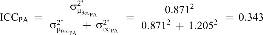
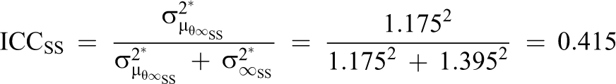
Thus, 34.3% of the long-range variance in PA and 41.5% of the long-range variance in SS is due to between-person variability.

In line with Voelkle et al. (2012), we computed p values by dividing the parameter estimate by its standard error to test for significance. All parameters except both cross-effects and both correlations are significantly different from zero (α = .05). As an effect size statistic for the (nonsignificant) cross-effects, we calculated the explained variance, R ², for derived discrete-time cross-lagged effects by comparing the derived process error variances from our reported model to the ones from a model where the respective cross-effect was set to zero. Just like the discrete-time cross-lagged effects, the explained variance depends on the length of the time interval. For the effect of PA on SS, the maximum R ² was .000664, whereas the effect size of SS on PA was essentially zero (R ² < 10⁻⁶). These are extremely small effect sizes which are unlikely to have any practical meaning.

Discussion

Cross-lagged models are routinely used in prevention research. However, as discussed in this article, the use of discrete-time cross-lagged panel models is associated with a number of problems that can be overcome by continuous-time modeling. Continuous-time models allow for using flexible longitudinal designs with unequally spaced measurement occasions, facilitate cross-study comparisons of results, and help exploring the unfolding of cross-lagged effects across different time intervals. In this article, we illustrated the use of a bivariate continuous-time model to investigate the dynamic interplay of PA and health, a classic research topic in prevention science. The most interesting effects in cross-lagged analyses are the cross-lagged effects. In the data from the “Midlife in the United States (MIDUS 2): Daily Stress Project, 2004–2009” (Ryff & Almeida, 2017), we found nonsignificant cross-lagged effects with extremely low effect sizes. Although our analysis was an illustrative example to highlight the advantages of continuous-time modeling, our results might add to the current state of research concerning the dynamic interplay of PA and health/pain, for which empirical evidence has been reported to be inconsistent and conflicting (e.g., Geneen et al., 2017; Sitthipornvorakul et al., 2011).

When interpreting our findings, however, several limitations need to be taken into consideration: (1) We only modeled average cross-effects. Persons might vary in the strength of the dynamic interplay of PA and health. In future studies, this should be investigated; this call for modeling random effects in cross-lagged models was also put forward by, for instance, Selig and Little (2012). (2) The time resolution in the analyzed data was rather low as the measurement of PA and SS was with respect to the last 24 hr. More fine-grained timing information, for instance, obtained from experience sampling and ambulatory assessment approaches might help to carve out effects more precisely. (3) Because the constructs were assessed with a single item, measurement error might be a problem (Selig & Little, 2012). In future studies, more reliable measurements could be used. (4) As a proxy for health (or sickness), we used the average score of physical SS ratings from the MIDUS 2 daily assessments. For differently framed and operationalized health and activity constructs, results may be different. (5) As this was a secondary analysis, the generalizability of our results is (mostly) determined by the sampling procedures and properties of the MIDUS 2 study. (6) We assumed stationarity, roughly speaking, this means that the variance and the mean of a process are constant over time. Furthermore, Bayesian estimation of continuous-time models is very slow (e.g., almost 3 days in our case). Future research should investigate how run time of such models could be reduced. One promising approach is illustrated by Hecht, Gische, Vogel, and Zitzmann (2019).

We presented a specific model from the class of continuous-time models that was suitable for the targeted research question. Many other variants of continuous-time models exist (e.g., van Montfort et al., 2018). Continuous-time models have, for example, been extended to include measurement models (e.g., Arminger, 1986; Boker, Neale, & Rausch, 2004; Chow, Lu, Sherwood, & Zhu, 2016; Deboeck & Boulton, 2016; Driver et al., 2017; Hamaker, Nesselroade, & Molenaar, 2007; Hecht, Hardt, et al., 2019; Oravecz, Tuerlinckx, & Vandekerckhove, 2011; Oud & Delsing, 2010; Oud & Jansen, 2000; Singer, 2012; Voelkle et al., 2012), to model random subject effects (e.g., Driver & Voelkle, 2018; Hecht, Hardt, et al., 2019; Oravecz & Tuerlinckx, 2011; Oud & Delsing, 2010), and for modeling nonstationary processes (e.g., Bandi & Phillips, 2010).

In conclusion, continuous-time models overcome some limitations of cross-lagged models and may help to gain a better understanding of dynamic interrelationships in prevention sciences.

Supplemental Material

Supplemental Material, JBD885026_ct.midus.bayes - Continuous-time modeling in prevention research: An illustration

Supplemental Material, JBD885026_ct.midus.bayes for Continuous-time modeling in prevention research: An illustration by Martin Hecht and Manuel C. Voelkle in International Journal of Behavioral Development

Supplemental Material

Supplemental Material, JBD885026_ct.midus.frequentist - Continuous-time modeling in prevention research: An illustration

Supplemental Material, JBD885026_ct.midus.frequentist for Continuous-time modeling in prevention research: An illustration by Martin Hecht and Manuel C. Voelkle in International Journal of Behavioral Development

Supplemental Material

Supplemental Material, JBD885026_midus.simulated - Continuous-time modeling in prevention research: An illustration

Supplemental Material, JBD885026_midus.simulated for Continuous-time modeling in prevention research: An illustration by Martin Hecht and Manuel C. Voelkle in International Journal of Behavioral Development

Footnotes

Funding

The author(s) declared receipt of the following financial support for the research, authorship, and/or publication of this article: We acknowledge support by the Open Access Publication Fund of Humboldt-Universität zu Berlin.

ORCID iD

Martin Hecht

Note

Appendix

References

Aaltonen

Latvala

Rose

R. J.

Kujala

U. M.

Kaprio

Silventoinen

(2016). Leisure-time physical activity and academic performance: Cross-lagged associations from adolescence to young adulthood. Scientific Reports, 6, 1–10. doi:10.1038/srep39215

Arminger

(1986). Linear stochastic differential equation models for panel data with unobserved variables. Sociological Methodology, 16, 187–212. doi:10.2307/270923

Bandi

F. M.

Phillips

P. C. B.

(2010). Nonstationary continuous-time processes. In Aït-Sahalia

Hansen

L. P.

(Eds.), Handbook of financial econometrics: Tools and techniques (pp. 139–201). Amsterdam, The Netherlands: Elsevier. doi.org/10.1016/B978-0-444-50897-3.50006-7

Becker

(2011). Sport zur Gesundheitsförderung oder treiben nur Gesunde Sport? [Sport for health promotion or do only healthy people engage in sports?]. Wiesbaden, Germany: VS Verlag für Sozialwissenschaften. doi:10.1007/978-3-531-92750-3

Bentler

P. M.

(1980). Multivariate analysis with latent variables: Causal modeling. Annual Review of Psychology, 31, 419–456. doi:10.1146/annurev.ps.31.020180.002223

Bergstrom

A. R.

(1988). The history of continuous-time econometric models. Econometric Theory, 4, 365–383. doi:10.1017/S0266466600013359

Boker

S. M.

Neale

Rausch

(2004). Latent differential equation modeling with multivariate multi-occasion indicators. In van Montfort

Oud

J. H. L.

Satorra

(Eds.), Recent developments on structural equation models (pp. 151–174). Dordrecht, The Netherlands: Kluwer Academic.

Bollen

K. A.

Curran

P. J.

(2006). Latent curve models: A structural equation perspective. Hoboken, NJ: Wiley-Interscience.

Bravata

D. M.

Smith-Spangler

Sundaram

Gienger

A. L.

Lin

Lewis

… Sirard

J. R.

(2007). Using pedometers to increase physical activity and improve health: A systematic review. Journal of the American Medical Association, 298, 2296–2304. doi:10.1001/jama.298.19.2296

10.

Carpenter

Gelman

Hoffman

M. D.

Lee

Goodrich

Betancourt

… Riddell

(2017). Stan: A probabilistic programming language. Journal of Statistical Software, 76, 1–32. doi:10.18637/jss.v076.i01

11.

Chambliss

D. F.

Schutt

R. K.

(2016). Making sense of the social world: Methods of investigation (5th ed.). Thousand Oaks, CA: Sage.

12.

Chow

S. M.

Sherwood

Zhu

(2016). Fitting nonlinear ordinary differential equation models with random effects and unknown initial conditions using the stochastic approximation expectation-maximization (SAEM) algorithm. Psychometrika, 81, 102–134. doi:10.1007/s11336-014-9431-z

13.

Cole

D. A.

Maxwell

S. E.

(2003). Testing mediational models with longitudinal data: Questions and tips in the use of structural equation modeling. Journal of Abnormal Psychology, 112, 558–577. doi:10.1037/0021-843X.112.4.558

14.

Collins

L. M.

Schafer

J. L.

Kam

C. M.

(2001). A comparison of inclusive and restrictive strategies in modern missing data procedures. Psychological Methods, 6, 330–351. doi:10.1037/1082-989X.6.4.330

15.

Deboeck

P. R.

Boulton

A. J.

(2016). Integration of stochastic differential equations using structural equation modeling: A method to facilitate model fitting and pedagogy. Structural Equation Modeling: A Multidisciplinary Journal, 23, 888–903. doi:10.1080/10705511.2016.1218763

16.

De Haan-Rietdijk

Voelkle

M. C.

Keijsers

Hamaker

E. L.

(2017). Discrete- vs. continuous-time modeling of unequally spaced experience sampling method data. Frontiers in Psychology, 8, 1–19. doi:10.3389/fpsyg.2017.01849

17.

Driver

C. C.

Oud

J. H. L.

Voelkle

M. C.

(2017). Continuous time structural equation modelling with R package ctsem. Journal of Statistical Software, 77, 1–35. doi:10.18637/jss.v077.i05

18.

Driver

C. C.

Oud

J. H. L.

Voelkle

M. C.

(2018). ctsem: Continuous time structural equation modelling (Version 2.7.6) [Computer software]. Retrieved from http://CRAN.R-project.org/package=ctsem

19.

Driver

C. C.

Voelkle

M. C.

(2018). Hierarchical Bayesian continuous time dynamic modeling. Psychological Methods, 23, 774–799. doi:10.1037/met0000168

20.

Farina

Tabet

Rusted

(2016). The relationship between habitual physical activity status and executive function in individuals with Alzheimer’s disease: A longitudinal, cross-lagged panel analysis. Aging, Neuropsychology, and Cognition, 23, 234–252. doi:10.1080/13825585.2015.1080213

21.

Gelman

Rubin

D. B.

(1992). Inference from iterative simulation using multiple sequences. Statistical Science, 7, 457–472.

22.

Geneen

L. J.

Moore

R. A.

Clarke

Martin

Colvin

L. A.

Smith

B. H.

(2017). Physical activity and exercise for chronic pain in adults: An overview of cochrane reviews. Cochrane Database of Systematic Reviews, 1, CD01127. doi:10.1002/14651858.CD011279.pub3

23.

Gollob

H. F.

Reichardt

C. S.

(1987). Taking account of time lags in causal models. Child Development, 58, 80–92.

24.

Granger

Di Nardo

Harrison

Patterson

Holmes

Verma

(2017). A systematic review of the relationship of physical activity and health status in adolescents. European Journal of Public Health, 27, 100–106. doi:10.1093/eurpub/ckw187

25.

Greenberg

D. F.

Kessler

R. C.

(1982). Equilibrium and identification in linear panel models. Sociological Methods & Research, 10, 435–451.

26.

Hamaker

E. L.

Nesselroade

J. R.

Molenaar

P. C. M.

(2007). The integrated trait-state model. Journal of Research in Personality, 41, 295–315. doi:10.1016/j.jrp.2006.04.003

27.

Hecht

Gische

Vogel

Zitzmann

(2019). Integrating out nuisance parameters for computationally more efficient Bayesian estimation – An illustration and tutorial. Structural Equation Modeling: A Multidisciplinary Journal. Advance online publication. doi:10.1080/10705511.2019.1647432

28.

Hecht

Hardt

Driver

C. C.

Voelkle

M. C.

(2019). Bayesian continuous-time Rasch models. Psychological Methods, 24, 516–537. doi:10.1037/met0000205

29.

Janssen

LeBlanc

A. G.

(2010). Systematic review of the health benefits of physical activity and fitness in school-aged children and youth. International Journal of Behavioral Nutrition and Physical Activity, 7, 1–16. doi:10.1186/1479-5868-7-40

30.

Kearney

M. W.

(2017). Cross-lagged panel analysis. In Allen

M. R.

(Ed.), The SAGE encyclopedia of communication research methods (pp. 312–314). Thousand Oaks, CA: Sage.

31.

Kim

D. E.

Yoon

J. Y.

(2017). The reciprocal causal relationship between social activities and health with reference to the cognitive function level among community-dwelling older adults: A cross-lagged panel analysis. Journal of Korean Academy of Community Health Nursing, 28, 13–22. doi:10.12799/jkachn.2017.28.1.13

32.

Kim

Noh

J. W.

Park

Kwon

Y. D.

(2014). Body mass index and depressive symptoms in older adults: A cross-lagged panel analysis. PLoS ONE, 9, 1–9. doi:10.1371/journal.pone.0114891

33.

Leonhardt

Lehr

Keller

Luckmann

Basler

H. D.

Baum

… Becker

(2009). Are fear-avoidance beliefs in low back pain patients a risk factor for low physical activity or vice versa? A cross-lagged panel analysis. GMS Psycho-Social-Medicine, 6, 1–12. doi:10.3205/psm000057

34.

Lindwall

Larsman

Hagger

M. S.

(2011). The reciprocal relationship between physical activity and depression in older European adults: A prospective cross-lagged panel design using SHARE data. Health Psychology, 30, 453–462. doi:10.1037/a0023268

35.

Neale

M. C.

Hunter

M. D.

Pritikin

J. N.

Zahery

Brick

T. R.

Kirkpatrick

R. M.

… Boker

S. M.

(2016). OpenMx 2.0: Extended structural equation and statistical modeling. Psychometrika, 81, 535–549. doi:10.1007/s11336-014-9435-8

36.

Oravecz

Tuerlinckx

(2011). The linear mixed model and the hierarchical Ornstein–Uhlenbeck model: Some equivalences and differences. British Journal of Mathematical and Statistical Psychology, 64, 134–160. doi:10.1348/000711010X498621

37.

Oravecz

Tuerlinckx

Vandekerckhove

(2011). A hierarchical latent stochastic differential equation model for affective dynamics. Psychological Methods, 16, 468–490. doi:10.1037/a0024375

38.

Oud

J. H. L.

Delsing

M. J. M. H.

(2010). Continuous time modeling of panel data by means of SEM. In van Montfort

Oud

J. H. L.

Satorra

(Eds.), Longitudinal research with latent variables (pp. 201–244). Berlin, Germany: Springer.

39.

Oud

J. H.

Jansen

R. A. R. G.

(2000). Continuous time state space modeling of panel data by means of SEM. Psychometrika, 65, 199–215. doi:10.1007/BF02294374

40.

Oud

J. H. L.

Voelkle

M. C.

(2014). Do missing values exist? Incomplete data handling in cross-national longitudinal studies by means of continuous time modeling. Quality & Quantity, 48, 3271–3288. doi:10.1007/s11135-013-9955-9

41.

R Core Team. (2018). R: A language and environment for statistical computing. (Version 3.5.2) [Computer Software]. Vienna, Austria: R Foundation for Statistical Computing. Retrieved from http://www.R-project.org/

42.

Read

Grundy

(2014). Allostatic load and health in the older population of England: A crossed-lagged analysis. Psychosomatic Medicine, 76, 490–496. doi:10.1097/PSY.0000000000000083

43.

Reiner

Niermann

Jekauc

Woll

(2013). Long-term health benefits of physical activity: A systematic review of longitudinal studies. BMC Public Health, 13, 1–9. doi:10.1186/1471-2458-13-813

44.

Ryff

C. D.

Almeida

D. M.

(2017). Midlife in the United States (MIDUS 2): Daily stress project, 2004–2009 [Data file, documentation, and code book]. Ann Arbor, MI: Inter-University Consortium for Political and Social Research. doi:10.3886/ICPSR26841.v2

45.

Selig

J. P.

Little

T. D.

(2012). Autoregressive and cross-lagged panel analysis for longitudinal data. In Laursen

Little

T. D.

Card

N. A.

(Eds.), Handbook of developmental research methods (pp. 265–278). New York, NY: The Guilford Press.

46.

Singer

(2012). SEM modeling with singular moment matrices Part II: ML-Estimation of sampled stochastic differential equations. The Journal of Mathematical Sociology, 36, 22–43. doi:10.1080/0022250X.2010.532259

47.

Sitthipornvorakul

Janwantanakul

Purepong

Pensri

van der Beek

A. J.

(2011). The association between physical activity and neck and low back pain: A systematic review. European Spine Journal, 20, 677–689. doi:10.1007/s00586-010-1630-4

48.

Stavrakakis

de Jonge

Ormel

Oldehinkel

A. J.

(2012). Bidirectional prospective associations between physical activity and depressive symptoms. The TRAILS study. Journal of Adolescent Health, 50, 503–508. doi:10.1016/j.jadohealth.2011.09.004

49.

Timmons

B. W.

LeBlanc

A. G.

Carson

Connor Gorber

Dillman

Janssen

… Tremblay

M. S.

(2012). Systematic review of physical activity and health in the early years (aged 0–4 years). Applied Physiology, Nutrition, and Metabolism, 37, 773–792. doi:10.1139/h2012-070

50.

Van Bree

R. J. H.

Bolman

Mudde

A. N.

van Stralen

M. M.

Peels

D. A.

de Vries

Lechner

(2017). Modeling longitudinal relationships between habit and physical activity: Two cross-lagged panel design studies in older adults. Journal of Aging and Physical Activity, 25, 464–473. doi:10.1123/japa.2016-0212

51.

Van de Schoot

Winter

S. D.

Ryan

Zondervan-Zwijnenburg

Depaoli

(2017). A systematic review of Bayesian articles in psychology: The last 25 years. Psychological Methods, 22, 217–239. doi:10.1037/met0000100

52.

Van Montfort

Oud

J. H. L.

Voelkle

M. C.

(Eds.). (2018). Continuous time modeling in the behavioral and related sciences. Cham, Switzerland: Springer.

53.

Voelkle

M. C.

Gische

Driver

C. C.

Lindenberger

(2018). The role of time in the quest for understanding psychological mechanisms. Multivariate Behavioral Research, 53, 782–805. doi:10.1080/00273171.2018.1496813

54.

Voelkle

M. C.

Oud

J. H. L.

(2013). Continuous time modelling with individually varying time intervals for oscillating and non-oscillating processes: Continuous time modelling. British Journal of Mathematical and Statistical Psychology, 66, 103–126. doi:10.1111/j.2044-8317.2012.02043.x

55.

Voelkle

M. C.

Oud

J. H. L.

Davidov

Schmidt

(2012). An SEM approach to continuous time modeling of panel data: Relating authoritarianism and anomia. Psychological Methods, 17, 176–192. doi:10.1037/a0027543

56.

Zitzmann

(2018). A computationally more efficient and more accurate stepwise approach for correcting for sampling error and measurement error. Multivariate Behavioral Research, 53, 612–632. doi:10.1080/00273171.2018.1469086

57.

Zitzmann

Hecht

(2019). Going beyond convergence in Bayesian estimation: Why precision matters too and how to assess it. Structural Equation Modeling: A Multidisciplinary Journal, 26, 646–661. doi:10.1080/10705511.2018.1545232

Supplementary Material

Please find the following supplemental material available below.

For Open Access articles published under a Creative Commons License, all supplemental material carries the same license as the article it is associated with.

For non-Open Access articles published, all supplemental material carries a non-exclusive license, and permission requests for re-use of supplemental material or any part of supplemental material shall be sent directly to the copyright owner as specified in the copyright notice associated with the article.

0.00 MB

0.07 MB

0.00 MB

0.07 MB

0.35 MB