
Abstract
Drawing inferences about dynamics of psychological constructs from intensive longitudinal data requires the measurement model (MM)—indicating how items relate to constructs—to be invariant across subjects and time-points. When assessing subjects in their daily life, however, there may be multiple MMs, for instance, because subjects differ in their item interpretation or because the response style of (some) subjects changes over time. The recently proposed “latent Markov factor analysis” (LMFA) evaluates (violations of) measurement invariance by classifying observations into latent “states” according to the MM underlying these observations such that MMs differ between states but are invariant within one state. However, LMFA is limited to normally distributed continuous data and estimates may be inaccurate when applying the method to ordinal data (e.g., from Likert items) with skewed responses or few response categories. To enable researchers and health professionals with ordinal data to evaluate measurement invariance, we present “latent Markov latent trait analysis” (LMLTA), which builds upon LMFA but treats responses as ordinal. Our application shows differences in MMs of adolescents’ affective well-being in different social contexts, highlighting the importance of studying measurement invariance for drawing accurate inferences for psychological science and practice and for further understanding dynamics of psychological constructs.
Keywords
Introduction
Intensive longitudinal data (ILD; e.g., Hamaker & Wichers, 2017) allow one to investigate the dynamics over time of latent (i.e., unobservable) psychological constructs. By frequently gathering data (say at more than 50 measurement occasions) of multiple subjects, new insights regarding subject-specific dynamics can be obtained, which have clinical implications. For instance, studies are being conducted on dynamics in emotions and behaviors related to mental health (e.g., Myin-Germeys et al., 2018; Snippe et al., 2016), and ILD can also be used to tailor interventions to the subject’s real-time dynamics of negative affect (van Roekel et al., 2017). Such data is efficiently gathered by means of Experience Sampling Methodology (ESM; Scollon et al., 2003), in which subjects repeatedly rate questionnaire items over several weeks, say five times a day, at randomized time-points. The recent steep increase in such datasets (e.g., Hamaker & Wichers, 2017; van Roekel et al., 2019) is related to novel technologies to efficiently gather these data with the use of smartphone apps. Hence, there is an urgent need to also develop novel analytical methods.
In order to draw valid inferences about the measured constructs, either for scientific or clinical purposes, it is crucial that the measurement model (MM) is invariant (i.e., constant) across time and subjects (i.e., having within- and between-person invariance). The MM indicates to what extent the latent constructs (or “factors”) are measured by which items, as indicated by the “factor loadings.” For continuous data, the MM is obtained by factor analysis (FA). If measurement invariance (MI) holds, the constructs are conceptually equal and thus comparable across subjects and over time. Often, MI is not tenable because response styles, substantive changes in item interpretation, or changes in the nature of the measured construct may affect the MM. That is, people may differ from each other in their MMs, for instance, depending on psychopathology, but one subject may also differ over time in its own MM, for instance, depending on the social context in which the questionnaire is filled in. When the non-invariance patterns are undetected or ignored, they cause a potential threat to valid inferences using standard methods for comparing factor means across time and subjects. For instance, changes in subjects’ overall emotional well-being may be (partly) due to changes in how subjects interpret the items. Changes in the MM are also important phenomena in their own right. For instance, detecting MM changes is crucial for valid decisions about treatment allocation over time and such changes may even signal the onset of a mental episode. Consider, for example, a psychologist who measures positive affect (PA) and negative affect (NA) in patients with a bipolar disorder. Patients in manic episodes often encounter high arousal PA such as feeling energetic or excited together with high arousal NA such as being irritated or distracted (American Psychiatric Association, 2013). This might result in a MM with one bipolar “arousal” factor contrasting “low” versus “high” arousal. When patients encounter depressive episodes, PA is generally lower and NA at least somewhat higher (Hamaker et al., 2010), which might correspond to a MM with two separate PA and NA factors or one bipolar “valence of affect” factor. Assessing MI thus allows for more accurate conclusions, but may also open up novel possibilities of early detection of subtle changes in daily functioning.
In order to assess for whom and when a MM applies, Vogelsmeier, Vermunt, van Roekel, and De Roover (2019) developed a novel method called latent Markov factor analysis (LMFA) for tracking and diagnosing MM changes for continuous responses in ILD. LMFA combines a latent Markov model (LMM; Bartolucci et al., 2014; Collins & Lanza, 2010) with mixture FA (McLachlan & Peel, 2000; McNicholas, 2016): The LMM clusters subject- and time-point-specific observations into a few dynamic latent classes or “states” according to the MMs underlying these observations and mixture FA evaluates which MM applies for each state. Thus, every state pertains to a different MM and the MM is invariant within one state. Note that not all MMs may apply to each subject. Some subjects may constantly stay in one state while others may transition between different states. By investigating the state memberships, one can see which subjects and measurements are comparable regarding their underlying MM. Investigating the state-specific MMs offers insights into the underlying dynamics and it also helps researchers make decisions about subsequent analyses. For example, when at least “partial” invariance holds across states (i.e., only a few MM parameters differ; Byrne et al., 1989), researchers could study discrete changes in factor means by repeating the LMLTA analysis, restricting invariant MM parameters to be equal across states, and adding factor means to the model.
The new method has raised awareness of possible MM changes in ILD among fundamental and applied researchers who are now eager to evaluate which MM applies to which subject at which time-point (Horstmann & Ziegler, 2020). However, an important limitation of LMFA is the assumption of having normally distributed continuous response items. This assumption is often violated in ILD. Although continuous items are sometimes used (e.g., participants are asked to give their answer by sliding on the Visual Analog Scale from 0 (“not at all”) to 100 (“very much”), many studies use multiple Likert items with five to seven categories for their assessment. Even though it has been shown that items with five or more categories might be treated as continuous (Dolan, 1994), it becomes problematic if the item response distributions are heavily skewed (e.g., when most responses have a 0 score, which is quite common with less frequent thoughts, emotions, or behaviors). FA is not robust against strong deviations from normality and, therefore, may yield inaccurately estimated parameters (Kappenburg-ten Holt, 2014; Rhemtulla et al., 2012; Vermunt & Magidson, 2005). Note that the same problem generally applies to studies that use ordinal items with less than five categories, although this is less common in ILD data. If the normal approximation is clearly incorrect, a better alternative is to treat the items as ordinal and to specify the probability of responding in a certain category by means of “item response theory” or “latent trait” (LT) models, where “trait” refers to a latent construct in the psychometric literature (Vermunt & Magidson, 2016).
The aim of this paper is to combine the strength of LT models to adequately deal with ordinal data with the strengths of LMFA to trace complex measurement non-invariance patterns in the data. The novel and much-needed latent Markov latent trait analysis (LMLTA) for ordinal data is obtained by replacing the mixture FA by a mixture multidimensional version of Muraki’s (1992) “generalized partial credit model” (GPCM) that treats the responses as ordinal. The second section describes LMLTA and how it compares to LMFA. The third section illustrates the empirical value of LMLTA to detect MM changes in ordinal data on adolescents’ well-being in different social contexts. Finally, the fourth section concludes with some points of discussion and future directions of research.
Method
Data Structure
In LMLTA, we assume intensive longitudinal observations that are nested within subjects and we assume multiple Likert and, therefore, ordinal items with response categories ranging, for instance, from
Latent Markov Latent Trait Analysis
In LMLTA, just as in LMFA, a LMM specifies transitions between discrete latent states (e.g., manic and depressive state) characterized by state-specific MMs (e.g., state 1 contains one arousal factor and state 2 two affect factors). A LMM is basically a latent class model (Lazarsfeld & Henry, 1968) and thus a method to find unobserved classes of observations with comparable response patterns. A LMM allows subjects to transition between latent classes over time, which is why the classes are called “states.” To get more insight into what possibly predicts state memberships, one may explore the relation between the state memberships and time-varying or time-constant explanatory variables or “covariates.” For instance, sleep quality and disruptions in the daily routine may increase the probability to transition to a manic state (Hamaker et al., 2010). The state-specific MMs are latent variable models that indicate which latent constructs are measured by which items and to what extent. The choice for the type of latent variable model directly follows from the assumed item response distribution: An LT model for ordinal data is used in LMLTA and a FA model for continuous data is used in LMFA.
The parameters in LMLTA can be estimated with the same approaches as in LMFA, using Latent GOLD (LG; Vermunt & Magidson, 2016) syntax. The first approach is a one-step full information maximum likelihood (FIML) estimation (Vogelsmeier, Vermunt, van Roekel, & De Roover, 2019) and the second approach is a three-step (3S) procedure that splits the estimation of the LMM and the state-specific MMs (Vogelsmeier, Vermunt, Bülow, & De Roover, 2019). The latter approach has advantages, especially regarding model selection with covariates. In the following, we first describe the LMM and then introduce the particular LT model applied in this paper and compare it to the FA model in LMFA. Thereafter, we discuss the two possible estimation procedures and the advantages of the 3S estimation.
Latent Markov model
The LMM is a probabilistic model with two assumptions (e.g., Bartolucci et al., 2014; Collins & Lanza, 2010): (1) The probability of being in state k (with
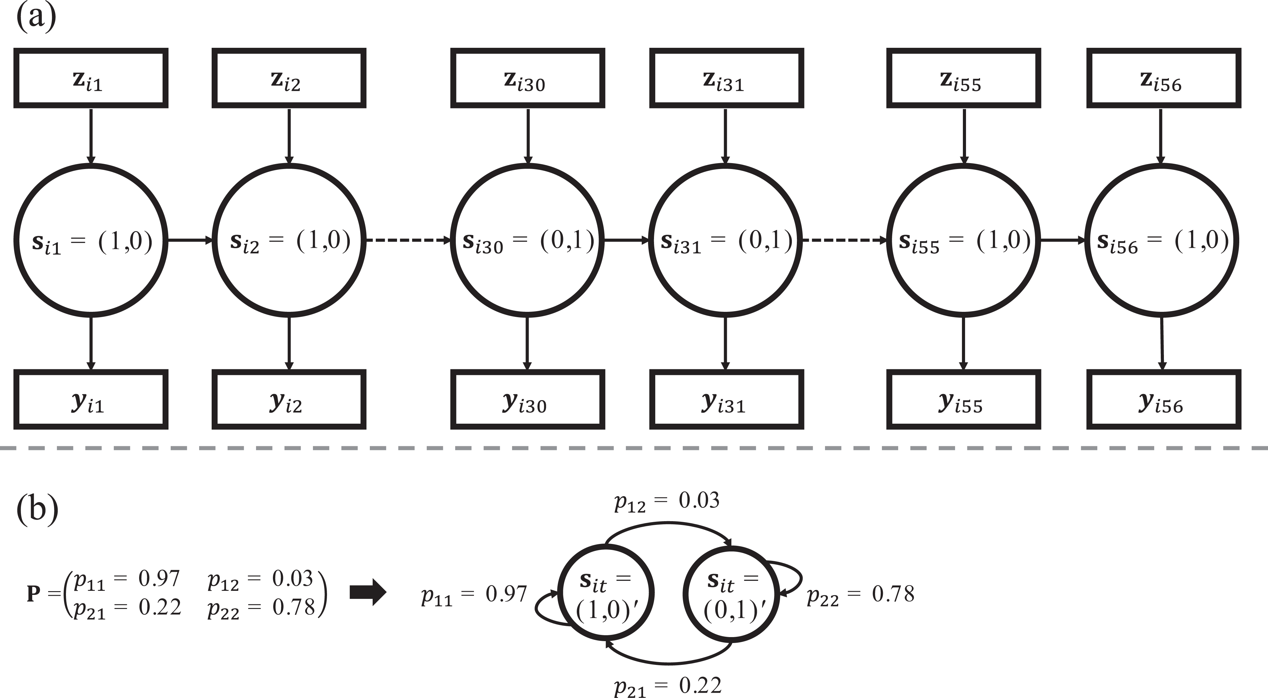
Part (a) is a graphical illustration of a latent Markov chain from the latent Markov latent trait analysis model. The binary vectors
A LMM is characterized by the “initial state,” “transition,” and “response” probabilities. Together, the parameters form the joint distribution of the observations and states. This is:
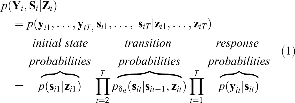
for subject i. The initial state and transition probabilities may depend on subject- and time-point-specific covariates
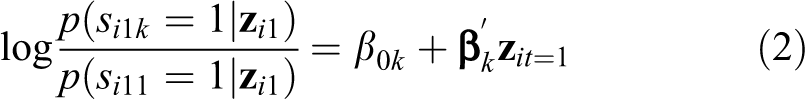
for
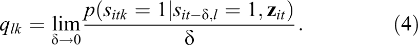
Transition probabilities are the probabilities to be in state
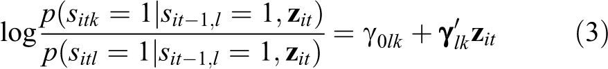
with
In the CT-LMM, the transition probabilities themselves are a function of the interval

Hence, covariates to predict any of the parameters (i.e., initial state and transition probabilities or intensities) are included by means of regression, as is usually done in LMMs (e.g., Bartolucci et al., 2014; Vermunt et al., 1999; Visser et al., 2009).
Instead of using only observed covariates in any of the parameters, one may also use a time-constant or time-varying latent categorical variable that classifies subjects according to their transition pattern or initial state probabilities into latent classes (Crayen et al., 2017; Vermunt et al., 2008). This “mixture (CT-)LMM” captures the most relevant between-subject differences in the transition process. The number of latent classes can be based on theory and interpretability or selected using information criteria such as the Bayesian information criterion (BIC, Schwarz, 1978) or the convex hull (CHull; Ceulemans & Kiers, 2006) method. An example is shown in the application (Application section).
Finally, the response probabilities
Measurement model
The MMs determine how the responses
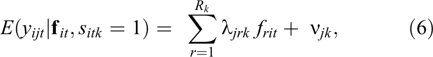
where Rk
is the state-specific number of factors,
In LMLTA, the ordinal responses
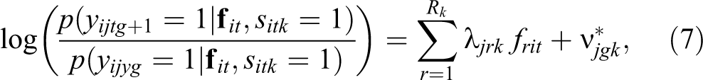
for
When comparing Equation (6) and Equation (7), the loading parameters for the FA model and the GPCM are clearly conceptually similar. In both cases, they indicate how strongly an item j measures a latent factor
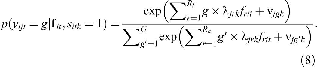
As in LMFA, the state-specific joint response probabilities for LMLTA at time point t are obtained by marginalizing over the latent factors. Moreover, the J item responses are assumed to be conditionally independent given the latent factors and the state membership. Therefore, the response probabilities are (e.g., Johnson & Bolt, 2010):
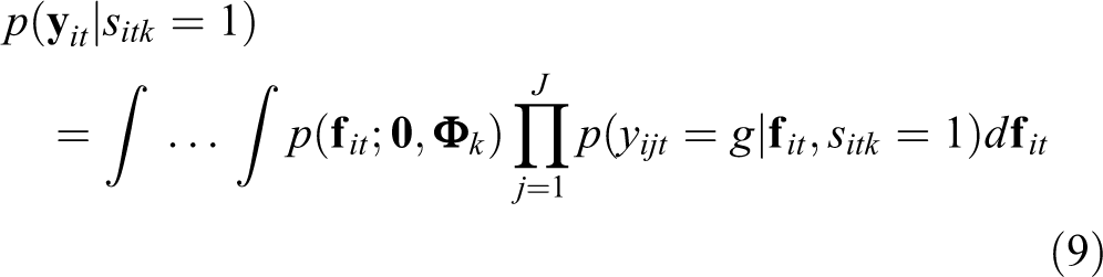
with
To enable the exploration of all kinds of MM changes, including the number and nature of the factors, an exploratory model is used in both methods. In contrast to a confirmatory model—in which certain factor loadings are assumed to be absent and therefore, set to zero—an exploratory model estimates all loadings.
1
However, both models are unidentified without further constraints. To partially identify the models and set a scale to the Rk
factors, one may restrict the factor means to zero and the factor (co)variances
As becomes apparent from Equation (6) and Equation (7), in either model, the state-specific MMs can differ in terms of the number of factors, the loadings, the intercepts, and the factor covariance matrices. However, there is an important difference between the two methods. In LMFA, states may also differ regarding unique variances, say
Besides this difference, MI analyses with FA and LT models are similar as their primary concern is to detect parameter differences. However, different words may be used to describe (non-) invariance. When using a LT model, researchers typically specify the lack of invariance, which is called “differential item functioning” (DIF). More specifically, “uniform DIF” is present when only intercepts differ, in our case across latent states, and “non-uniform DIF” is present when loadings differ across states, whether intercepts are equal or not (Bauer, 2017). In contrast, when using a FA model, researchers typically specify which level of invariance has been reached, starting from an invariant number of factors and pattern of zero loadings, followed by invariant loadings, intercepts, and finally unique variances (Meredith, 1993). In the next paragraph, we will describe how to obtain the estimates that are used to investigate the level of invariance in LMLTA.
Maximum likelihood estimation
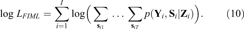
The parameters in LMLTA are obtained with maximum likelihood (ML) estimation. One may choose between (1) the one-step FIML estimation and (2) the 3S estimation, just as is the case for LMFA. However, estimating the LMLTA model with either approach is computationally more complex than estimating the LMFA model. Therefore, LMLTA is limited regarding the number of factors that can be estimated (i.e., including more than three factors is usually unfeasible; see Appendix B for detailed explanations). First, for the FIML estimation (Vogelsmeier, Vermunt, van Roekel, & De Roover, 2019), the following loglikelihood function, derived from the joint distribution in Equation (1), has to be maximized:
In LG, the ML estimates are obtained with the forward-backward algorithm (Baum et al., 1970), which is an efficient version of the Expectation Maximization algorithm (Dempster et al., 1977), tailored to LMMs. Additionally, in the Maximization step, a Fisher algorithm is used to update the log-intensities and a combination of the Expectation Maximization and the Newton-Raphson algorithm (De Roover et al., 2017) is used to update the state-specific MM parameters.
Second, the 3S estimation (Vogelsmeier, Vermunt, Bülow, & De Roover, 2019) builds upon Vermunt’s (2010) ML method and decomposes the estimation into three steps. First, in step 1, the state-specific MMs are obtained with a mixture GPCM while treating repeated measures Estimating state-specific MMs (disregarding the dependence of the observations). Assigning observations to the states (depending on the most likely state membership). Estimating the (mixture) CT-LMM with fixed MMs (correcting for step 2’s classification error).
The 3S estimation is almost as good as the FIML estimation in terms of parameter estimation. Only the state recovery is slightly worse and the standard errors can be slightly overestimated (Vogelsmeier, Vermunt, Bülow, & De Roover, 2019). 5 Apart from that, the 3S approach comes with several advantages. First, step-wise procedures are more intuitive for researchers who use complex methods such as LMLTA or LMFA to analyze their data because it is in line with how they prefer to conduct their analyses (Vermunt, 2010). That is, they see the investigation of the different MMs underlying their data as a first step and the investigation of subject’s transitions between the MMs over time as well as the exploration of possible covariate effects as a next step.
Second, LMLTA (like LMFA) is an exploratory method, which entails that the best number of states k and factors per states Rk
has to be determined. To this end, a large number of (plausible) models has to be estimated and compared by means of loglikelihood-based criteria that consider fit and parsimony. The evaluation of model selection criteria in LMLTA is beyond the scope of this article but, based on previous findings for related methods (Bulteel et al., 2013; Vogelsmeier, Vermunt, van Roekel, & De Roover, 2019), we suggest to use the BIC in combination with the CHull and compare the three best models in terms of interpretability. Note that CHull balances fit and parsimony without making distributional assumptions and, thus, may perform better for some empirical datasets. In the FIML estimation, the number of models to be compared grows fast. For example, there are nine models when comparing models with one to three states and one to two factors per state. When adding different (sets of) covariates to the CT-LMM, the nine models have to be re-estimated for every set of covariates (e.g.,
Third, the FIML estimation takes several hours for each model while the 3S estimation is usually done in less than 30 minutes. This makes the FIML estimation less desirable, or even unfeasible, when researchers want to explore several covariate effects on MM changes. For all these reasons, we employ the 3S estimation in this study (for details, see Online Supplement S.1).
Application
Data
The data stem from a larger “Grumpy or Depressed?” study, which aimed to assess whether daily mood profiles (i.e., variability in affect) would predict the risk for depression in adolescents in the long run as recent work has indicated that the short-term dynamics could be linked to long-term psychopathology (e.g., Maciejewski et al., 2019; for a description of the study, see, e.g., de Haan-Rietdijk et al., 2017; Janssen et al., 2020; van Roekel et al., 2019). Briefly, during three 7-day measurement bursts or “waves” (with approximately 3-month intervals in between), 250 Dutch adolescents (12 to 16 years old) completed up to eight questionnaires per day at random moments (median interval: 2.25 hours). 8 Out of the 250 adolescents, 164 participated in all three waves, 38 in two of the waves and 48 in one of the waves. In total, the adolescents completed 14,432 questionnaires.
Measures
For each assessment, adolescents indicated the degree to which 12 affect items applied to them (see Table 1) using 7-point Likert items (ranging from
The dataset contains several covariates but, in this study, we focused on the social context and depression as we found these variables particularly interesting to relate to possible MM changes: Emotional experiences may vary depending on the social context. For instance, adolescents may experience elevated positive mood when being among friends, whereas they may be somewhat more irritable and unhappy in the company of their parents, and more demotivated at school (Kendall et al., 2014; Soenens et al., 2017; van Roekel et al., 2013). For some adolescents, mood may be context-independent. Firstly, some adolescents could be in an overall positive mood regardless of the social context (Dietvorst et al., under review). Secondly, adolescents with a depression and those at risk for developing a depression may be rather stable in their emotions in that they often feel unhappy and irritable in any social context (Dietvorst et al., under review; Kendall et al., 2014; Silk et al., 2011). Therefore, for some adolescents, we expect a particular state membership to be more likely in one social context than in another, but also that adolescents differ in their state membership stability, for example, based on their depression level.
Description of the Applied Mixture CT-LMLTA Model
We will examine the context-dependency of state memberships by regressing the transition intensities (as defined in Equation (5)) on the social context covariates when estimating the CT-LMM (in step 3 of the estimation). To capture potential between-adolescent differences in stability, we will include a latent class variable that automatically classifies the adolescents based on their transition patterns, making the model a mixture CT-LMM as briefly introduced in the Latent Markov Latent Trait Analysis section. To see how many different patterns there are, we will compare models with one to three classes in terms of their fit by means of the BIC and CHull. Note that adolescents are allowed to transition to another class at the beginning of each wave—because subjects may change in their transition patterns over time (possibly related to their wave-specific depression scores—such that the latent class variable is, strictly speaking, another state variable modeled via a DT-LMM (note that a DT model makes sense here as the intervals between the waves are approximately the same for all adolescents). To prevent confusion with the MM state, we will just refer to this latent variable as “class,” with
The specification of the initial class (for
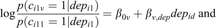

respectively. Note that this application is meant to illustrate the empirical value of tracing MM changes with LMLTA. No hypotheses were pre-registered and all analyses are exploratory so that interesting findings should be validated in future research before drawing any conclusions.
Obtaining and Investigating the Results of the Mixture CT-LMLTA Model
Below, we follow the three consecutive steps of the 3S estimation described in Latent Markov Latent Trait Analysis section.
Step 1 & 2: Estimating state-specific MMs & assigning observations to the states
Model selection
To select the best fitting model, we conducted the mixture GPCM analysis for models with one to three states and one to two factors per state (i.e., nine models 10 ). Considering one to two factors not only preserves computational feasibility but also makes sense for affect questionnaires as PA and NA are often found as primary affect dimensions that may collapse into one bipolar factor if the emotions are strongly negatively related (Dejonckheere et al., 2018; Vogelsmeier, Vermunt, Bülow, & De Roover, 2019). We selected the model with two states and two factors in each state because it was the best according to the BIC and among the two best models according to the CHull (for model selection details, see the Online Supplement S.2; for the syntax of the selected model, see Online Supplement S.4). Forty-two percentage of the observations belonged to MM 1 and 58% to MM 2.
Results and interpretation
To examine the between-state MM differences, we first looked at the state-specific loadings in Table 1. Note that we modeled the covariance matrices in both states. To set the factor scales, we set the loadings of the items “happy” on factor 1 and “unhappy” on factor 2 equal to 1 in both states. To eliminate rotational freedom, we set the remaining loadings of the same items equal to zero. This has led to a well-interpretable simple structure. State 1 is characterized by separate PA and NA factors that correlated negatively (
Differences in Factor Loadings, Factor (Co-)Variances, Factor Correlations, and Item Means Across the two States.
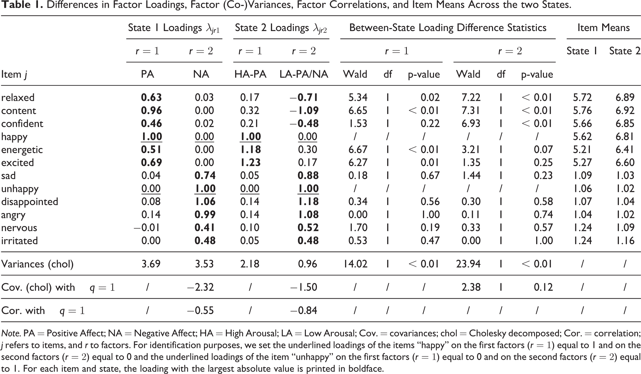
Note. PA = Positive Affect; NA = Negative Affect; HA = High Arousal; LA = Low Arousal; Cov. = covariances; chol = Cholesky decomposed; Cor. = correlation; j refers to items, and r to factors. For identification purposes, we set the underlined loadings of the items “happy” on the first factors (
Next, we investigated the between-state differences in the mean item scores. These scores are directly related to the state- and category-specific intercepts (which are given in Supplement 3 Table 2), but the item means are easier to interpret. They are calculated as
Step 3: Estimating the mixture CT-LMM with fixed MMs
Since each adolescent may have a different MM at different measurement occasions, we examined adolescents’ transitions from one state to another. Additionally, as motivated above, we investigated (1) whether adolescents differed in their state- (and thus MM-) memberships by classifying the adolescents based on their transition patterns (i.e., transitions between states from one measurement occasion to the next) into latent classes that could differ across the three waves, (2) whether the wave-specific covariate depression had an influence on this class membership, and (3) whether the time-varying social context covariates (family, classmates, and friends) affected the transitions between the states and whether these effects differed across classes. To this end, we estimated the mixture CT-LMM with the state assignments from step 2 of our analysis as indicators, while accounting for the inherent classification errors. Note that the correction was hardly necessary as the classification errors were very small due to a high state separation (with
Model selection
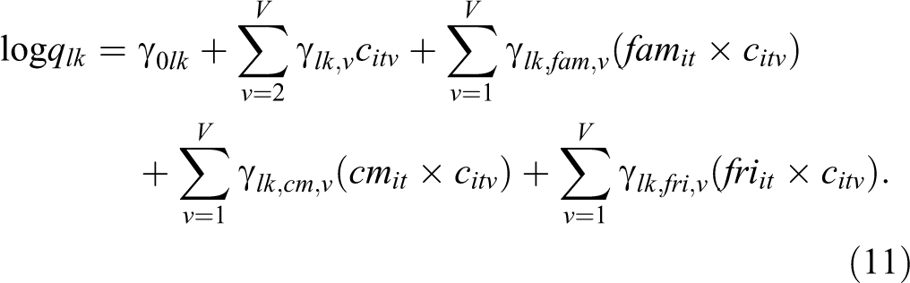
We first estimated the “full” model as summarized in Equation (11) and (12) for one to three classes (i.e., with all possible covariates as just described). In the two- and three-class solutions, the effects of depression on the initial class (
Results and interpretation
Table 2 shows the parameters of the final model. First, we looked at the three classes that captured differences in adolescents’ between-state transitions. To this end, we computed the probabilities for the median interval (2.25 h) and mean covariate values: 14
Parameter Estimates for the Mixture CT-LMM in Step 3 of LMLTA.
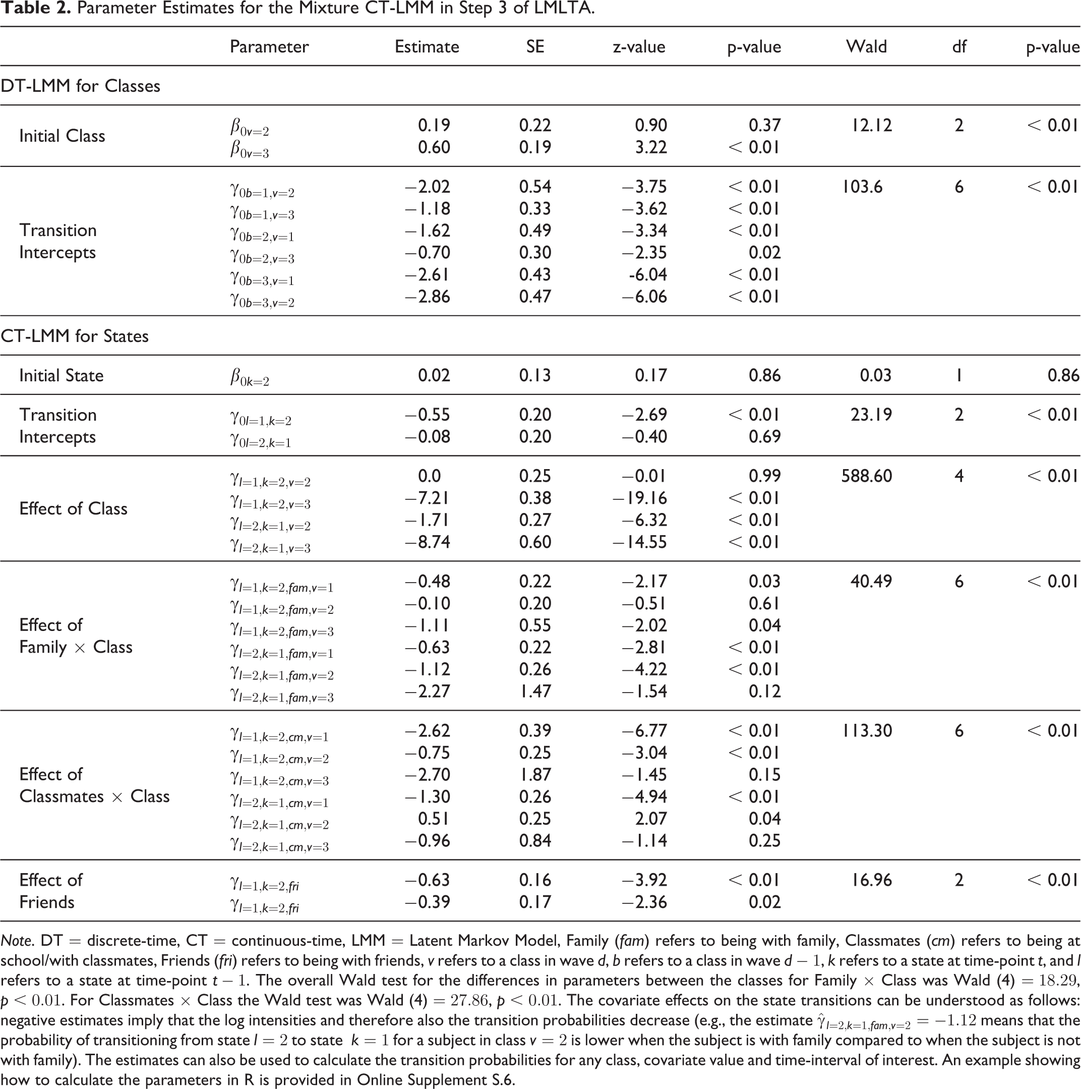
Note. DT = discrete-time, CT = continuous-time, LMM = Latent Markov Model, Family (
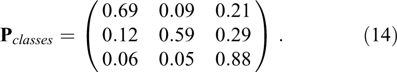
Class 1 and 2 each include 25% of the adolescents, whereas 50% were assigned to class 3. As can be seen from the relatively large values in column 1 of
Thus, over the three waves, adolescents developed a more stable assessment of their feelings. Perhaps their repeated answers to the questionnaire helped them to develop emotional awareness.
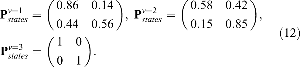
Considering the most prominent results (i.e.,
For adolescents in class 1, being with classmates decreased both the probability of moving to state 2 and moving to state 1 (
In all three classes, being with friends (compared to not being with friends) decreased the probability of moving to state 2 (
Summary of the LMLTA findings
We conclude that two MMs were underlying adolescents’ responses: in state 1 (42% of all observations), adolescents distinguished mainly between PA and NA and had a slightly worse mood than in state 2 (58% of all observations), where adolescent distinguished more between LA-PA (e.g., content) and HA-PA (e.g., excited) than they did between (LA-)PA and NA; (2) three state-transition patterns were found, implying that adolescents indeed differed in the stability of their emotional experience: in class 1, adolescents frequently transitioned between the states with a high probability to be in state 1; in class 2 they frequently transitioned but were more likely to be in state 2, and in class 3, they mainly stayed in one of the two states; (3) depression did not influence the class membership and thus the transition pattern; (4) for the unstable classes 1 and 2, being with family increased the probability to be in state 1; (5) for class 1, being with classmates increased the probability of staying in either state; (6) for all classes, being with friends—and for class 2, being with classmates—increased the probability to be in state 1. Our results show that researchers can obtain valuable insights from investigating MM changes and that it is important to consider the possibility that changes in positive or negative affect (e.g., evaluated by means of investigating changes in sum scores) could come from variability in the underlying MMs. Therefore, the novel method LMLTA (or LMFA) can improve the emerging trend of studying emotional dynamics as predictors of future well-being and psychopathology. In the future, it would be interesting to study the MMs and transition patterns in a larger group of adolescents with (different levels of) depression and to include other covariates that may explain differences in transition patterns and state-membership probabilities. For example, stress can cause a simplified representation of emotions (Dejonckheere et al., 2019), which can lead to very high correlations between emotions.
Discussion
In recent years, the awareness of potential measurement model (MM) changes in intensive longitudinal data—and the associated comparability problems—increased among substantive researchers and they are keen to evaluate such changes with new methods like latent Markov factor analysis (LMFA) (Horstmann & Ziegler, 2020). Understanding subject- and context-dependent MMs in more detail may benefit future studies on daily life dynamics and also have clinical implications, for instance, when MMs can be related to the onset of psychopathology. However, up to now, only researchers whose data contained (approximately) normally distributed continuous items could benefit from LMFA, whereas intensive longitudinal data often contain ordinal item responses with few categories or skewed distributions. In this article, we combined the strength of LMFA to evaluate MM changes over time with the strength of latent trait (LT) models accommodate ordinal data in the new latent Markov latent trait analysis (LMLTA).
We showed that LMFA and LMLTA are similar as they both capture discrete changes or differences in subjects’ underlying MM and thus in how latent constructs are measured by observed item responses. The difference lies in the type of latent variable model that is used to specify the relations between the latent constructs and observed variables, which directly follows from the assumed distribution of the observed item responses. Whereas the factor analysis (FA) model in LMFA assumes normally distributed continuous item responses, the generalized partial credit model (GPCM) in LMLTA assumes ordinal responses. The GPCM differs from the FA model in that (1) it has one intercept per item category and not one per item, (2) error variances cannot be freely estimated as they need to be fixed for identification, (3) rotation is only possible by means of setting identifying constraints, and (4) the number of constructs that can be included in the model is limited due to the computationally more complex estimation. This implies that, in LMLTA, more parameters have to be estimated, error variances are assumed to be identical across states, and the model specification is less flexible than in LMFA. For these reasons, we believe that LMFA should be the preferred method if the items are approximately normal and are measured with at least five categories (Dolan, 1994). The robustness of LMFA against violations of normality has never been evaluated, however. In the future, it would therefore be important to formulate more concrete guidelines on the basis of a simulation study that is tailored to intensive longitudinal data and that provides information on the robustness of LMFA, for instance, in terms of sample size and number of measurement occasions, degree of skewness, and number of item response categories. In the meantime, researchers should be cautious and, in case of doubt, opt for LMLTA and compare its results to those of LMFA.
By investigating differences in discrete MM changes over time in relation to covariates, LMLTA is a valuable step toward validly studying psychological dynamics. Additionally, as briefly described in the introduction, the results of LMLTA may also help researchers decide on subsequent analyses. When invariance is clearly untenable, further evaluating dynamics with an approach that builds upon the invariance framework is simply not appropriate. However, observations for which invariance holds can be used to study dynamics in latent processes with standard analyses (e.g., growth models, Muthén, 2002, or dynamic structural equation modeling, Asparouhov et al., 2017), without results being influenced by differences in the underlying MMs. Moreover, if partial invariance holds across states, one may also continue with latent process analyses either by removing items with non-invariant parameters or by allowing for state- (or subject- and time-point-) specific parameters. Finally, we would like to highlight that there is no gold standard yet in how to analyze intensive longitudinal data and the latent variable framework that LMLTA is based on is only one possibility. There are various other reasonable frameworks for analyzing the data (e.g., network psychometrics; Epskamp, 2020; Marsman et al., 2018) and decisions about the data analysis can considerably impact, for example, clinical recommendations (Bastiaansen et al., 2020). Therefore, in the future, it would be desirable to compare perspectives about psychological phenomena from various modeling approaches.
Supplemental Material
Supplemental Material, Accepted_VogelsmeierEtal2020_LMLTA_highlightedSupplement - Latent Markov Latent Trait Analysis for Exploring Measurement Model Changes in Intensive Longitudinal Data
Supplemental Material, Accepted_VogelsmeierEtal2020_LMLTA_highlightedSupplement for Latent Markov Latent Trait Analysis for Exploring Measurement Model Changes in Intensive Longitudinal Data by Leonie V. D. E. Vogelsmeier, Jeroen K. Vermunt, Loes Keijsers and Kim De Roover in Evaluation & the Health Professions
Footnotes
Appendix A
Declaration of Conflicting Interests
The author(s) declared no potential conflicts of interest with respect to the research, authorship, and/or publication of this article.
Funding
The author(s) disclosed receipt of the following financial support for the research, authorship, and/or publication of this article: The research leading to the results reported in this paper was sponsored by the Netherlands Organization for Scientific Research (NWO) [Research Talent grant 406.17.517; Veni grant 451.16.004; Vidi grant 452.17.011]. Funding for data collection came from Utrecht University, Dynamics of Youth seed project, awarded to Loes Keijsers, Manon Hillegers et al.
Supplemental Material
Supplemental material for this article is available online.
Notes
References
Supplementary Material
Please find the following supplemental material available below.
For Open Access articles published under a Creative Commons License, all supplemental material carries the same license as the article it is associated with.
For non-Open Access articles published, all supplemental material carries a non-exclusive license, and permission requests for re-use of supplemental material or any part of supplemental material shall be sent directly to the copyright owner as specified in the copyright notice associated with the article.