
Abstract
Accurate assessment of perfusion in vital organs like the pancreas is crucial for monitoring various pathologies, particularly tumors and their growth. While tumor growth inhibition usually results in decreased vascularization, current techniques for non-invasive and cost-effective perfusion assessment lack sufficient vessel separability for pancreatic applications, hindering optimal treatment selection and monitoring. Ultrasound (US) imaging offers advantages like low cost, rapid acquisition, non-invasiveness, and non-ionizing radiation. However, speckle, patient-related and acquisition-related motion artifacts, and limitations in distinguishing contrast-enhanced blood vessels, particularly in single frames, pose significant challenges. This study presents a novel solution utilizing image analysis of US contrast agents (UCAs) to characterize vascularization. The approach involves data denoising, selection of static frames, spatio-temporal registration, and deconvolution. The post-processed images are analyzed based on temporal intensity changes and normalized to extract trends. Data from 13 patients undergoing chemotherapeutic treatment with FOLFIRINOX or gemcitabine/abraxane were analyzed. Though no direct effects on vascularization are expected, the results suggest a correlation between derived vascularization trends (based on B-mode and CEUS data) and observed clinical treatment outcomes. Four patients exhibited negative slope (related to vascularization regression) aligned with clinical improvement, while six showed positive slope (related to increased vascularization) coinciding with treatment deterioration. Two patients displayed negative slopes without clinical improvement, and one patient displayed positive slope but had clinical improvement. These findings indicate the potential of this method to estimate treatment efficacy and guide personalized therapy, although the sample size is small and further investigation is warranted.
Keywords
Introduction
P
Pancreatic cancer, predominantly adenocarcinoma (accounting for approximately 90% of cases 2 ), is a highly aggressive disease associated with a poor prognosis. 3 One-year survival rates are 25%, dropping to 5% to 22% at 5 years.4,5 Risk factors include smoking, obesity, diabetes, and certain genetic conditions. 6 Diagnosis is challenging due to late-stage symptoms and involves imaging, blood tests, and biopsy.6 -11
Currently, surgical resection remains the primary curative treatment option for patients with pancreatic cancer, however fewer than 20% of patients are eligible for this intervention. The primary objective of surgery is to achieve complete tumor resection, ensuring no microscopic cancer cells remain at the primary tumor site. This objective is often complicated by the inherent poor vascularization characteristic of PDAC. 12
For patients with unresectable PDAC, treatment options may include chemotherapies such as Gemcitabine/Abraxane or FOLFIRINOX treatments to help shrink the tumor and manage symptoms. If the treatment demonstrates efficacy and results in significant tumor regression, surgical intervention may become a viable option.
To optimally treat PDAC patients, tumor staging is a crucial step. The staging of pancreatic cancer is based on the results of helical CT and tumor-node-metastasis classification according to the most recent edition of the “American Joint Committee on Cancer.” The goal of CT imaging is to determine the position and size of the tumor, the involvement of veins and arteries, and the presence of metastasis.
Stages I and II typically include tumors confined to the pancreas with minimal or no involvement of major vessels. Tumors of stage III are extended beyond the pancreas, involving the superior mesenteric vein, portal vein or splenic vein. Stage IV tumors involve the superior mesenteric artery or celiac axis.
Tumor stage serves as a critical determinant for assessing resectability. Stage I and II are considered resectable, stage II to III tumors are borderline resectable pancreatic cancer (BRPC), depending on whether a safe and complete resection and the reconstruction of the affected veins and arteries are possible. Stage IV tumors are metastatic PDAC and are considered non-resectable.
Precise tumor staging allows clinicians to provide the optimal treatment to the patients based on the advancement of the disease. 12
Ultrasound, a non-invasive and real-time imaging modality, holds significant promise for monitoring PDAC stage due to its ability to visualize subtle changes in tissue morphology, vascularity, and local tumor invasion, offering a cost-effective and accessible alternative for disease progression assessment. 13
Ultrasound Contrast Agents
Contrast agents, used in contrast enhanced ultrasound (CEUS) imaging, are designed to enhance signal and provide real-time insights into tissue morphology and vascularization. 14 Ultrasound contrast agents (UCAs) consist of gas-filled microbubbles that are injected intravenously to enhance ultrasound images. These microbubbles produce a signal enhancement of 20 to 30 dB due to their distinct acoustic impedance compared to the surrounding tissues.14,15 To ensure stability, the microbubbles consist of a shell made of lipids, proteins or polymers, to encapsulate gases such as perfluorobutane. 14 These microbubbles, typically 1 to 5 µm in diameter, are small enough to circulate through capillaries and allow visualization of microvasculature.14,16 The microbubbles oscillate non-linearly in response to ultrasound waves, creating a strong acoustic backscatter that enhances contrast in imaging. 14 CEUS can also be used for treatment augmentation.
Treatment Augmentation by Sonoporation
PDAC is characterized by a dense stromal environment, known as desmoplasia, which not only supports tumor growth but also creates a physical and immunological barrier that limits drug delivery and immune cell infiltration. 17 This tumor characteristic has prompted the use of sonoporation as a strategy to overcome the physical barriers to drug delivery.
In this study population, sonoporation (cellular sonication), the use of ultrasonic waves to increase the permeability of the cell plasma membrane by oscillating microbubbles (cavitation), was employed in order to increase the permeability of the drugs through the vasculature. Previous studies suggested that trans-abdominal CEUS can be employed for improved drug delivery18,19 in pancreatic cancer treatment.
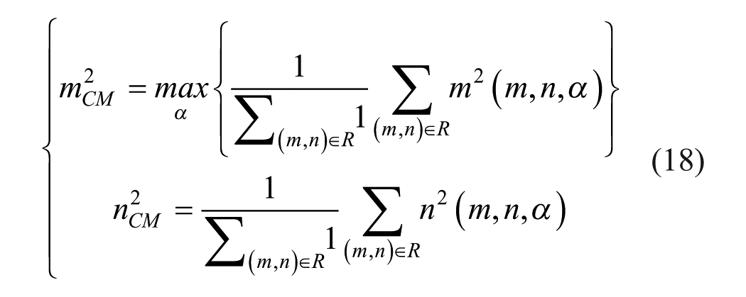
Vascularization Assessment for Treatment Evaluation
Despite the potential of CT perfusion imaging for PDAC treatment monitoring, accurate assessment faces several challenges, including the highly desmoplastic tumor microenvironment which impedes contrast agent delivery and washout, the heterogeneous nature of tumor perfusion, and the difficulty in distinguishing viable tumor from post-treatment fibrotic changes. Furthermore, standardization of imaging protocols, kinetic models, and quantitative parameters across different modalities and centers remains a significant hurdle for widespread clinical implementation. 20
CEUS presents several advantages in the study of pancreatic cancer. Notably, it facilitates the differentiation between various subtypes of solid pancreatic lesions based on their distinct contrast enhancement patterns. 21 Furthermore, CEUS aids in the differential diagnosis of pseudocysts and cystic tumors. 22 CEUS provides a robust assessment of tissue vascularization in humans.23 -25
This work aims to enable the estimation of treatment efficacy based on vascularity analysis in readily obtainable CEUS data:
- investigate the use of CEUS for treatment monitoring in patients undergoing chemotherapy treatment augmentation by sonoporation.
- investigate the potential of CEUS to predict treatment response.
Objectives
This research investigates the use of CEUS to visualize pancreatic perfusion, associating it with pancreatic cancer status to evaluate treatment outcomes. The treatment is standard-of-care chemotherapy, augmented with a sonoporation process. The perfusion assessment assumes vascularity changes according to tumor status but not as a direct effect from anti-angiogenesis drugs, since the therapeutics medicines used in this work are not anti-angiogenesis.
The hypothesis: Treatment response is expected to result in decreased vasculature and perfusion while the opposite is expected from non-responders.
The clinical research conducted by our collaborators in Philadelphia and Bergen is designed to enhance drug permeability within the pancreas utilizing sonoporation. Our research, which focuses on the vascularity assessment, constitutes a component of this collaborative and comprehensive endeavor.
The broader field has explored various applications of ultrasound in pancreatic cancer, such as analyzing vascular invasion through ultrasound 26 and evaluating response to treatment with high intensity focused ultrasound (HIFU). 27 Herein, we aim to estimate the response to a non-invasive treatment using conventional (non-HIFU) ultrasound instrumentation, leveraging our developed image processing pipeline. The purpose of this research is to estimate treatment response with the use of CEUS-derived metrics. In an environment where it is challenging to obtain sufficient amount of data for machine learning (ML) methods.
Phantom
To validate the research methodologies, a preliminary evaluation was conducted on a phantom. This phantom setup was used to test the image processing algorithm, including its vascularization assessment capabilities.
Methods
Clinical Trial
As part of an ongoing Phase II clinical trial on augmenting standard-of-care chemotherapeutic regimens with sonoporation, an analysis of a subset of active subjects was conducted. The subset was defined by a minimum of three finished treatment sessions, to enable the establishment of preliminary trendlines for changes. Sessions were spaced approximately 2 weeks apart. The clinical trial was approved by the institutional review boards (IRBs) of both Thomas Jefferson University in Philadelphia, USA and Haukeland Hospital in Bergen, Norway, as well as by the Food and Drug Administration (FDA), with investigational new drug (IND) number 153874, and registered with CliniclTrials.gov, with national clinical trial (NCT) number 04821284.
The trial evaluates the safety and efficacy of the two standard-of-care chemotherapies Gemcitabine/Abraxane or FOLFIRINOX treatments of patients with inoperable adenocarcinoma of the pancreas, comparing augmentation with Sonazoid™ (UCA) and ultrasound treatment to chemotherapy alone.
It should be noted that the mentioned medicines are not expected to directly change the vascularity.
Patients
The patients enrolled in this study were diagnosed with Stage II or higher PDAC and were scheduled for standard-of-care chemotherapy. Subjects were then randomized (1:1 ratio) into two groups: The first group was treated with standard-of-care chemotherapy alone (control group), while the other group received standard-of-care chemotherapy combined with sonoporation to enhance the delivery of therapeutics. Data from 13 patients from the experimental group have been analyzed.
Technical Details
Patient data were acquired with a C1–6 curved linear probe using LOGIQ™ E10 scanner (GE HealthCare, Waukesha, WI, USA). Acquisitions were performed for B-mode and contrast imaging employing transducer frequencies of 2.5 and 4 MHz correspondingly, in dual imaging mode. 60 seconds video clips were recorded to capture the UCA wash-in phase. Imaging depths, ranging from 6 to 13 cm, were selected based on patient body habitus. The acquisition frame rate was 8 Hz, and the mechanical index (MI) was 0.10 to 0.20. Images were captured with resolutions of either 748 × 1346 or 900 × 1442 pixels (Rows × Columns) in a 4-D (Y, X, RGB, Time) uint8 (

Each patient underwent a series of sonoporation treatments, which continued until either surgical intervention was possible or the patient could no longer comply with the treatment, typically due to chemotherapy side effects or PDAC progression. The imaging protocol included:
- B-mode scan during wash-in, from arrival and 60 seconds on.
- Initiation of Sonazoid™ infusion (rate of 0.18 ml/kg/h).
- CEUS scan during wash-in, from arrival and 60 seconds on.
- Sonoporation treatment augmentation for 20 minutes.
The algorithm code developed for this study was implemented in MATLAB® (R2019a).
Phantom
A custom phantom (Figure 1) with simulated vessels was fabricated in our laboratory. During fabrication, we optimized the agarose stiffness and minimized air bubbles (noise). This involved iterative adjustments of agar concentration, heating temperature, stirring, cooling, and degassing. Polytetrafluoroethylene tubes (200 µm inner diameter, 450 µm outer diameter) were chosen to mold simulated vessels to be perfused with microbubbles and were removed before imaging to avoid signal interference. SonoVue®28 which was readily available, was used instead of Sonazoid™, due to budgetary constraints. SonoVue® microbubbles (2–8 µm diameter, mean 2.5 µm) were selected for their size compatibility with human capillary networks (<7 µm) and biocompatibility.14,16 The microbubbles consist of a phospholipid/polyethylene glycol (PEG) shell (biocompatible), filled with sulfur hexafluoride gas (SF6, safe and clinically used). 28
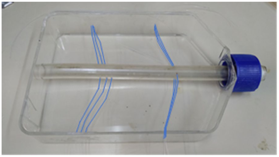
The phantom’s structure with marked tubes.
While it is not optimal to use different UCAs, the difference in performance is considered negligible for the purposes of this study. Their mean diameters are of a similar order of magnitude (Sonazoid™: 1–5 µm diameter, mean 2.1 µm), and the phantom study served solely for the calibration of the image processing algorithm, requiring only fundamental microbubble properties rather than the specific chemical attributes of the contrast agents.
Phantom data were acquired with the following parameters:
- Manufacturer: GE Healthcare Ultrasound.
- Model Name: Vivid S70, Transducer: Linear 9L.
- Width/Columns: 1016 (pixels), Height/Rows: 708 (pixels).
- dx: 0.00511 (cm/pixel), dy: 0.00511 (cm/pixel).
- Cine Rate: B-mode 24 (frames/second), CEUS 30 (frames/second).
- Transducer Frequency: B-mode 10 (MHz), CEUS 4 (MHz).
- MI: 0.1
Data Analysis
The algorithm (Figure 2) presented herein integrates a combination of features and functionalities to establish a framework designed to predict treatment outcomes based on CEUS data from several treatment sessions, thereby, ideally, facilitating informed decision-making in early stages. A detailed explanation of the algorithm components is provided in subsequent sections.
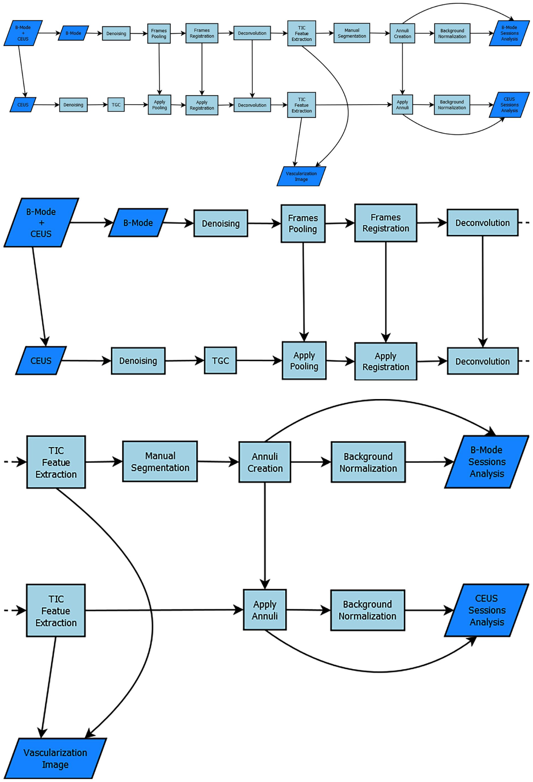
A scheme of the different functions forming the algorithm’s structure. Top—full scheme, middle—data preparation zoom-in (left half of the scheme), bottom—feature extraction zoom-in (right half of the scheme).
The algorithm’s workflow involves the following key steps:
- Preparation: Multiplicative model → Wavelet denoising → Time Gain Compensation → Frames selection → Registration.
- Analyzing: Segmentation → Deconvolution → Maximum Intensity Projection + Time-Intensity Analysis.
- Conclusion: Normalization → Estimation.
Denoising
Multiplicative model
To maximize information extraction from CEUS images, comprehensive preprocessing is essential. This involves understanding and removing inherent noise sources, while preserving image fidelity. Common noise sources include electronic noise, background tissue, and breathing motion. 29
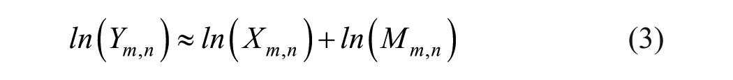
The primary challenge in denoising US images, excluding various artifacts, stems from the speckle pattern. Speckle arises from the inherent characteristics of ultrasound wave scattering 30 within the imaged tissue. This phenomenon which can be modeled as multiplicative, non-Gaussian noise (2) poses a significant denoising challenge compared to additive noise.

Where
To convert the multiplicative model into an additive model a logarithmic transformation is applied (3), which yields a Gaussian-like additive noise with a zero mean
The logarithmic image (denoted by
Wavelet decomposition
Although various speckle filters exist, wavelet denoising (WD) provides a powerful alternative. WD has demonstrated advantages upon alternatives in speckle reduction and contrast enhancement in ultrasound images.
29
WD utilizes wavelets, small wave-shaped functions that act as building blocks for signal analysis. However, for effective signal decomposition and reconstruction, these wavelets must possess unique mathematical properties: square-integrability (
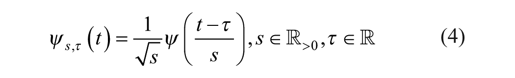

where
Convolution of the signal with wavelet function will extract its coefficient in the same wavelet space, meaning:

Wavelet decomposition utilizes a two-step filtering process: high-pass filter (HPF) and low-pass filter (LPF) followed by down sampling. The original image undergoes row-wise filtering, separating detail and approximation components. Subsequent down sampling by a factor of 2 reduces the resolution. The resulting sub-images are further filtered column-wise with HPF and LPF, followed by down sampling. This process yields four decomposed images represented by wavelet coefficients. A universal threshold is then applied for further analysis.
Threshold
Wavelet thresholding for denoising employs two main strategies: sub-band and global thresholding. Sub-band thresholding estimates noise variance in horizontal, vertical, and diagonal sub-bands at each decomposition level. This estimation starts from the outer spectral bands (higher levels) and progresses inwards. Threshold values are then calculated using the Visu shrinkage rule. 32 In contrast, global thresholding estimates noise variance only in the diagonal band, but the resulting threshold is applied to all sub-bands (horizontal, vertical, and diagonal). This approach leverages the assumption that the diagonal band holds most high-frequency components and consequently, higher noise content. Notably, thresholding is not applied to the approximation level to avoid reconstruction artifacts.
The thresholding process, also referred to as “wavelet shrinkage,” utilizes various techniques: hard, soft, semi-soft (firm), and stretch thresholding. The effectiveness of shrinkage hinges on the sparsity of the wavelet coefficients, with most coefficients ideally being zero. 32
This work employs soft thresholding of a universal threshold for denoising. Soft thresholding avoids artifacts that might arrive with hard thresholding, due to its sharp changes in coefficient values. We utilize the bior4.4 wavelet and determine the decomposition level (denoising level) based on the minimum of two criteria:
Soft thresholding:
Visu shrinkage rule is thresholding by applying universal threshold. The universal threshold:

where the threshold
The estimated local noise variance
This threshold is based on the fact that for a zero mean independent and identically distributed (IID) Gaussian process with variance
Time gain compensation (TGC)
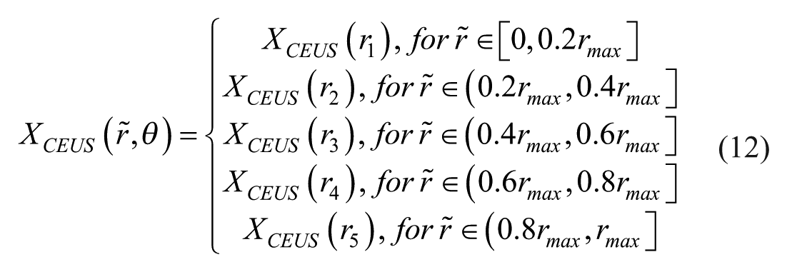
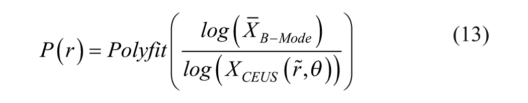
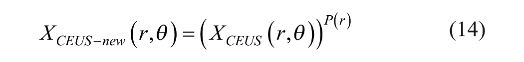
Due to signal attenuation, CEUS data exhibits depth-dependent signal reduction. To address this, an adaptive enhancement system (correction for TGC) is employed. It divides the image (with intensity values of double [0,1]) into five axial depth levels of equal size. Histograms are then calculated for each level, including their lateral extensions. From these histograms, the mean intensity value for each depth level is extracted. The B-mode image’s log-transformed mean value is subsequently divided by the log-transformed mean values of the CEUS image. Finally, a fourth-degree polynomial is fitted to these five normalized values, and the image is adjusted using this polynomial (similar to adaptive gamma correction).
Frames selection
Following noise reduction, frames for analysis were selected from B-mode video as the most static frames compared with a pre-selected B-mode frame (the reference frame). The corresponding CEUS frames for analysis were chosen based on the same temporal indices as their B-mode counterparts. This reference frame showcases the clearest visualization of the tumor and was selected by an experienced radiologist. Frame selection was based on cross-correlation with the reference frame. Only frames exhibiting high correlation were then combined (typically neighboring frames or those within the same phase in the physiological cycle, such as breathing or heartbeat), resulting in a new video clip with a sequence of maximally static frames relative to the reference (Figure 3).
The frames selection is applied by normalized cross-correlation (NCC):
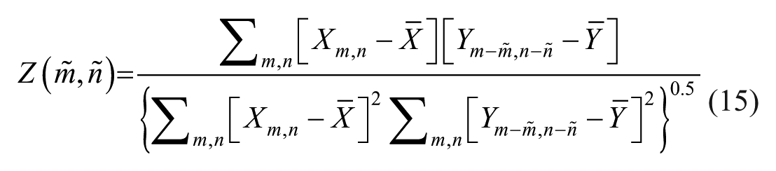

Where
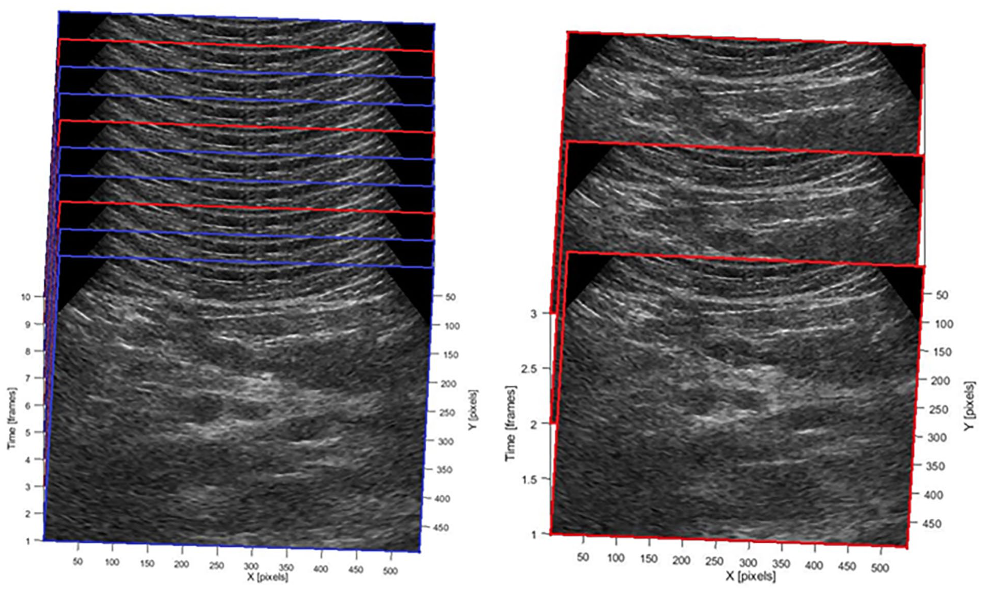
A scheme of the frames’ selection. On the left image there are red and blue edges frames. The red edges represent images with high cross-correlation. On the right there are only the red edges frames left.
A dual-thresholding system is employed to identify robust matches. Initially, cross-correlated frames are ranked in descending order based on their NCC values. The top 10% of frames exhibiting the highest correlation values are retained. Subsequently, this subset of frames is further filtered to include only those with NCC values exceeding 0.66 (~2/3, as it avoids different organs positions, and keeps enough frames for analysis), ensuring a minimum level of correlation for all selected frames.
These threshold values were determined to establish a meaningful selection process. The initial percentile-based threshold aims to capture a small but sufficient number of the highest-correlating frames for subsequent analysis. The second absolute threshold is intended to ensure that the selected frames exhibit a substantial level of static similarity, while remaining sufficiently inclusive for analysis given the available data. It is important to note that these thresholds were not subjected to formal optimization through training due to the limited dataset.
The remaining video clips are therefore in the length of
Registration
Following frame selection, image registration further reduces motion artifacts within the video clip. Frame selection rearranges frames and sets a threshold, while registration attempts to align all frames to a chosen reference frame and to preserve key information. This is achieved using a non-rigid pyramid method with four levels and three iterations.33,34 Deformation fields are calculated based on the B-mode video (assumed less noisy) and then applied to the corresponding CEUS frames within the same clip. This approach leverages the assumption that both modalities experience similar deformations due to their near-simultaneous acquisition from the same anatomical region.
For the phantom study, B-mode and CEUS data were acquired sequentially due to the controlled experimental conditions. Conversely, in the patient cohort, simultaneous acquisition of B-mode and CEUS images was performed, with a temporal resolution of
Segmentation
Lesion segmentation on video clips (Figure 4) was performed manually by a physicist and a radiologist in consensus. This segmentation was specifically conducted on the B-mode images, with simultaneous reference to the correlated activity observed in the CEUS data.
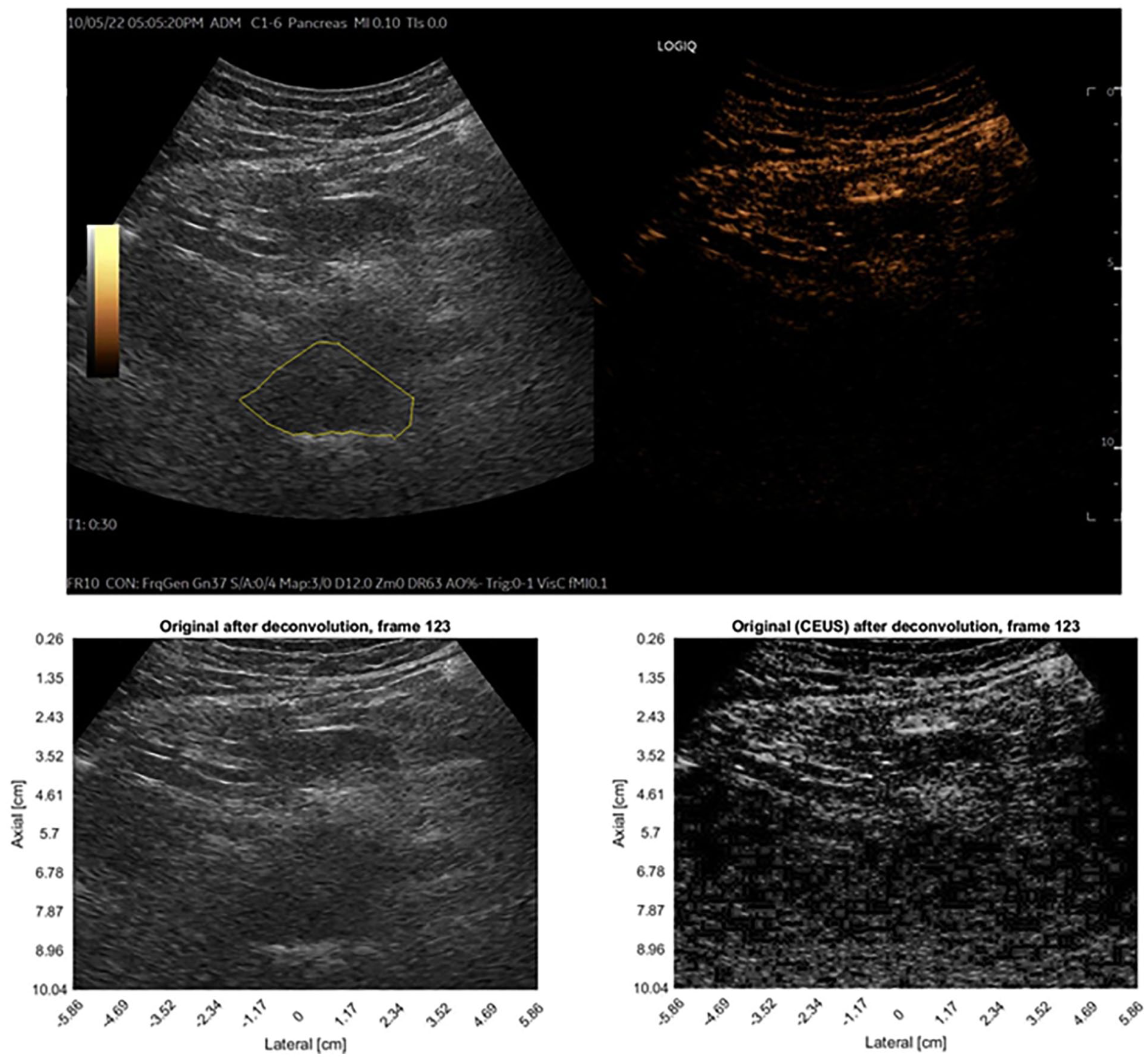
Top—The original video format, prior to the analysis (patient 003, session 2). Tumor contoured in yellow, appears hypoechoic (dark) on B-mode US. bottom—post-processing images of B-mode (left) and CEUS (right).
A new segmentation was performed in each session.
Polygon
To expedite the manual segmentation process within the analysis workflow, a custom graphical user interface (GUI) was developed. This facilitated the creation of high-fidelity lesion masks using polygon territory marking (manually selected dots, connected with straight continuous line to form a closed polygon shape) within the B-mode video clips themselves (Figure 5).
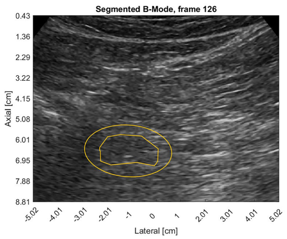
Example segmentation of a tumor. The inner polygon (center) marks the lesion. The elliptic ring bounds its surroundings.
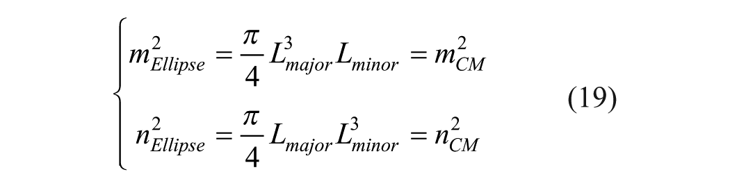
Ellipse
To incorporate information of the microenvironment surrounding the tumor, and additional subregion was selected. Based on a simplistic assumption that the tumors are elliptically shaped, an elliptic fit is first applied based on the polygonal tumor region and then a concentric ring system is derived based on the ellipse, in order to dilate the tumor contour and incorporate the surrounding tumor microenvironment.
The center of mass of the region (pixel fractions):
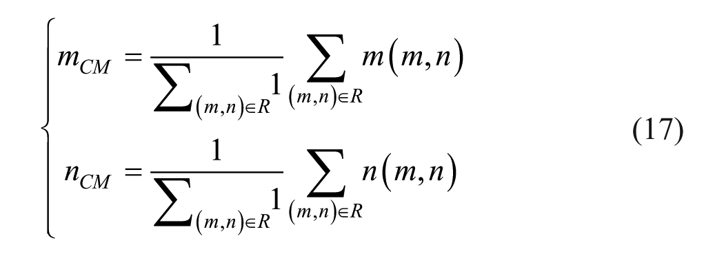
Where
Where
Ring
Lesion analysis employed a concentric ring system derived from an inscribed ellipse. Ring radii were determined in centimeters (not pixels) to ensure consistent spacing. This approach created rings with a constant radial distance of 0.5 cm between their inner and outer boundaries (Figure 5).
Deconvolution
Resolution
Beyond speckle, the inherent PSF of the imaging system fundamentally limits spatial resolution, potentially obscuring fine details. To mitigate this effect, several methods were explored, including maximum intensity projection (MIP), temporal compounding (TC), and deconvolution.
Approaches
Deconvolution offers several approaches to address image resolution limits imposed by the PSF. The most intuitive method is inverse convolution. This technique assumes a known PSF, representable as a matrix due to convolution properties. By applying the Moore-Penrose pseudoinverse of the PSF matrix to the image, inverse convolution aims to recover a more realistic image (sharper). Inverse convolution, while intuitive, suffers from sensitivity to noise amplification due to the inverse matrix properties.
ML methods 35 can achieve promising results in deconvolution but typically necessitate extensive labeled datasets comprising both PSFs and their corresponding ground truth TRFs. Acquiring such a large dataset was not feasible within the scope of this clinical trial. Instead, we propose an iterative deconvolution method.
Iterative deconvolution
The iterative deconvolution process aims to restore the tissue reflectivity function (TRF) image, from the given point spread function (PSF) image.
The process is explained in the following sections:
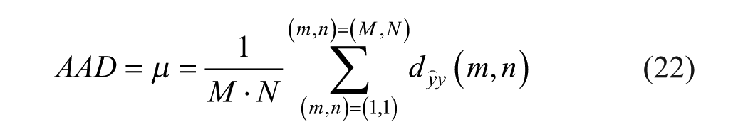
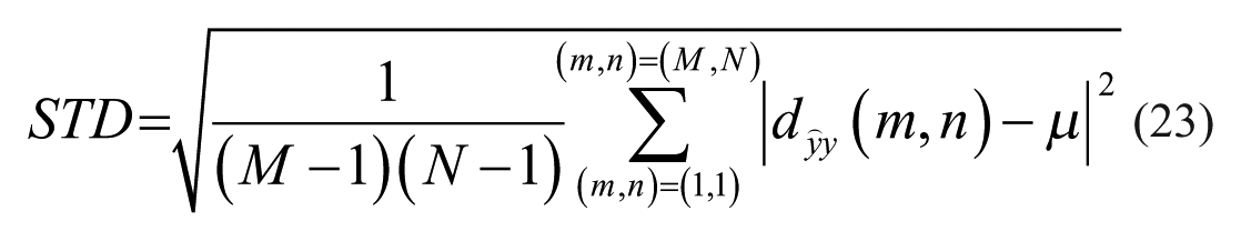
Loss
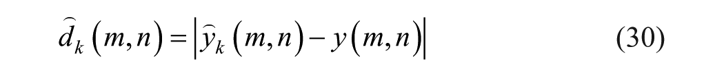
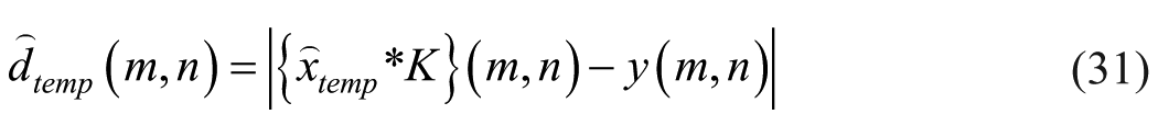
The criteria employed for comparing the different reconstruction methods were maximal absolute difference (MAD), average absolute difference (AAD), standard deviation (STD) of absolute difference and root mean square (RMS) of absolute difference. All of the above are calculated pixel-wise on the difference image (20) between the reconstructed image (the forward convolution of the TRF image) and the PSF image:


Where
Kernel
The initial assumption of the kernel was a 2-dimensional (2-D) normalized Gaussian:

Where
A small part of the PSF image is chosen to include a local peak of intensity, and it is used for the calibration of the kernel’s properties (
Iterations
The first deconvolution iteration sets a reduced intensity version of the original image (by soft thresholding) as the TRF image, for initial sparsity. The following deconvolution steps are applied by iterations up to a sufficient result (a pre-defined difference threshold) or reaching the iterations limit. After each iteration equation (29), the change value decreases, so that the TRF image would converge (Figure 6).
Each pixel in the temporary deconvolved image (the TRF image) is checked for improvement in its matching reconstructed pixel as well as in its nearest neighbors (local difference image), before accepting the change. This improvement is measured by minimizing the absolute difference between the original image and the temporary reconstructed image. If the change of the observed pixel minimizes the temporary local difference image (compared to its effect on its neighbors) the change is chosen. This pixel then changes its value by the change value of the current iteration.

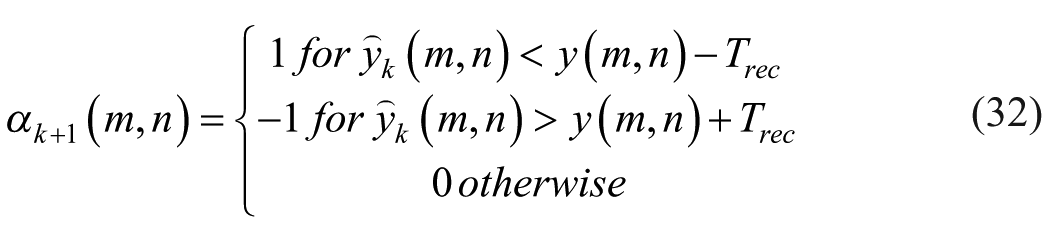
Where
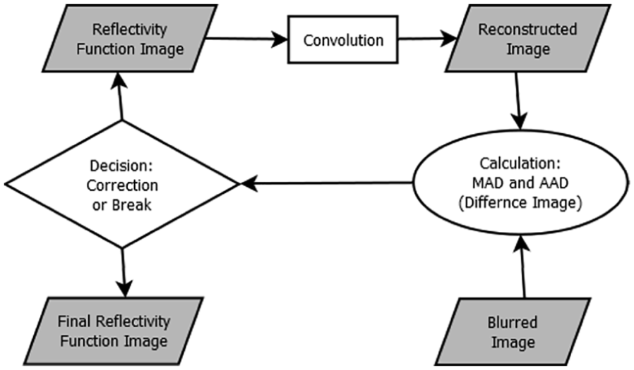
The iterative algorithm diagram.
Considering the limitations of noise sensitivity and data requirements, the iterative deconvolution method was chosen for its ability to achieve user-defined accuracy with an estimated PSF.
Perfusion Assessment
Maximum Intensity Projection (MIP)
MIP is a commonly employed tool for visualizing and analyzing blood flow. Its effective application necessitates several stringent conditions: a static transducer position, a constant acquisition angle, and spatially stationary organs. These conditions are frequently unmet in dynamic clinical settings. Additionally, MIP assumes negligible high-frequency, high-intensity noise artifacts. While valuable for visualizing sparse contrast agent flow paths, these limitations render MIP less suitable for quantitative US perfusion assessment. Thus, here it was combined with time intensity analysis (TIA) to improve its performance.
Time-Intensity Analysis (TIA)
The TIA approach analyzes the temporal intensity changes within a region of interest (ROI) to characterize the temporal behavior of observed UCA. In CEUS, TIA can be used to assess the temporal behavior of different tissues based on their characteristic echo patterns (hyperechoic, hypoechoic, etc.) or movement patterns. This analysis leverages established knowledge of UCA dynamics and tissue behavior in US images. We focused here on: maximum, mean, standard deviation, and difference between sessions. In this way the analysis was not significantly compromised by the frames’ selection. From these features we composed fusion images:
- “structure analysis” image represents the mean B-mode after registration (a.r.).
- “vascularity analysis” image is a composite of the MIP CEUS after deconvolution (a.d.) merged with the standard deviation (STD) CEUS after registration (a.r.).
Both fusion images are calculated pixelwise, by multiplying each element of both images with each other, which keeps the same range of values ([0,1]⋅[0,1]→[0,1]).
Quantification
Perfusion quantification currently lacks standardized criteria due to varying measurement conditions. Therefore, for this study, the spatial average intensity within a defined region of interest (ROI) was chosen as the primary metric. This ROI was measured in previous and subsequent frames, within the selected frames, for its temporal analysis. For assessing long-term trends related to treatment and lesion progression, comparisons were drawn between different video clips (different treatment sessions). However, given that each video clip possesses slightly different properties (e.g., mean intensity, noise levels), the chosen perfusion quantification method necessitates normalization for meaningful interpretation.
Normalization
Perfusion quantification relies on the average intensity of the time-dependent images, within a defined ROI. To facilitate comparisons across treatment sessions with varying probe settings, a normalization process was implemented. This involves dividing all intensity (of ROI) measures (mean and standard deviation) by the background intensity (mean of the whole sectional image) from the same session while accounting for depth and processing condition (original, registered, or deconvolved). This approach enables comparisons between sessions with a common baseline.
However, it is important to acknowledge limitations. While normalization can reveal deviations above or below baseline, significant background variations across sessions may obscure trends in isolated segment values. Observed trends may not hold true if background intensities differ substantially. The normalization method assumes that total image intensities represent both mean (background) intensity and segments intensities, as multiplications of the former. The multiplication coefficients represent the trend. Additionally, it assumes intensity values do not reach saturation before or after normalization.
Classification
The fusion images include dynamic information from the video clip and are cropped to the ROIs of the tumor and its most adjacent ring and averaged, and the same process goes for the whole image, for normalization. Following the normalization, the derived intensity values, combined with the standard deviation values, from the longitudinal treatment sessions were plotted against time (different sessions). Linear regression analysis was then applied to these data points to determine the temporal trend of vascularity within the treatment sessions, as indicated by the slope of the regression line.
The areas analyzed comprised the tumor volume and its immediately adjacent peritumoral ring, assuming this annulus (yellow ring in Figure 5) forms the best representation of the external tumor vessels. Three types of normalized mean images were combined (averaged) in order to balance their properties. These images were the original image (“before registration”), the registered image (“after registration”) and the deconvolved image (“after deconvolution”). These averaged images were cropped by the tumor area and its surrounding ring and averaged in these areas, on both the B-mode and the CEUS videos, creating four values per treatment session for temporal plot.
The four resulting slope values, corresponding to these regions, were subsequently summed, and this aggregate slope value served as the basis for classification. The different slopes were summed to produce a single classification value that incorporates all inputs while remaining simple enough to minimize the risk of overfitting. The assumption made here is that an increased slope (sum) is correlated with an increased vascularity and thus with a disease progression, and vice versa (decreased slope ↔ decreased vascularization ↔ treatment response). Progression is assessed by the medical oncologists’ team based on CT results (tumor size), biomarkers (CA19-9) and tumor activity (PET imaging) combined. Responders were selected for surgery.
This rudimentary classification approach was selected to demonstrate proof of concept rather than to achieve optimal classification accuracy. Furthermore, this simplified method was chosen to mitigate the risk of overfitting the limited dataset that a more complex classification model might introduce.
Several operations were employed to extract the results 29 :
- Mean squared error (MSE) was utilized for the creation of the slopes trendlines when fitting to the data from different sessions.
- The final results (increased/decreased vascularity) were compared with the clinical outcome reported by the attending clinicians.
Results
Phantom
To ensure the algorithm’s accuracy and usefulness, a comprehensive analysis process (Figure 7, Table 1) was performed on a custom-made agar-based phantom. This analysis followed the processes detailed in the Denoising, Deconvolution, Perfusion Assessment, sections. The ground truth mask image was calculated as the active pixels (non-zero STD) in the phantom B-mode video, assuming both the phantom and the transducer were spatially fixed.
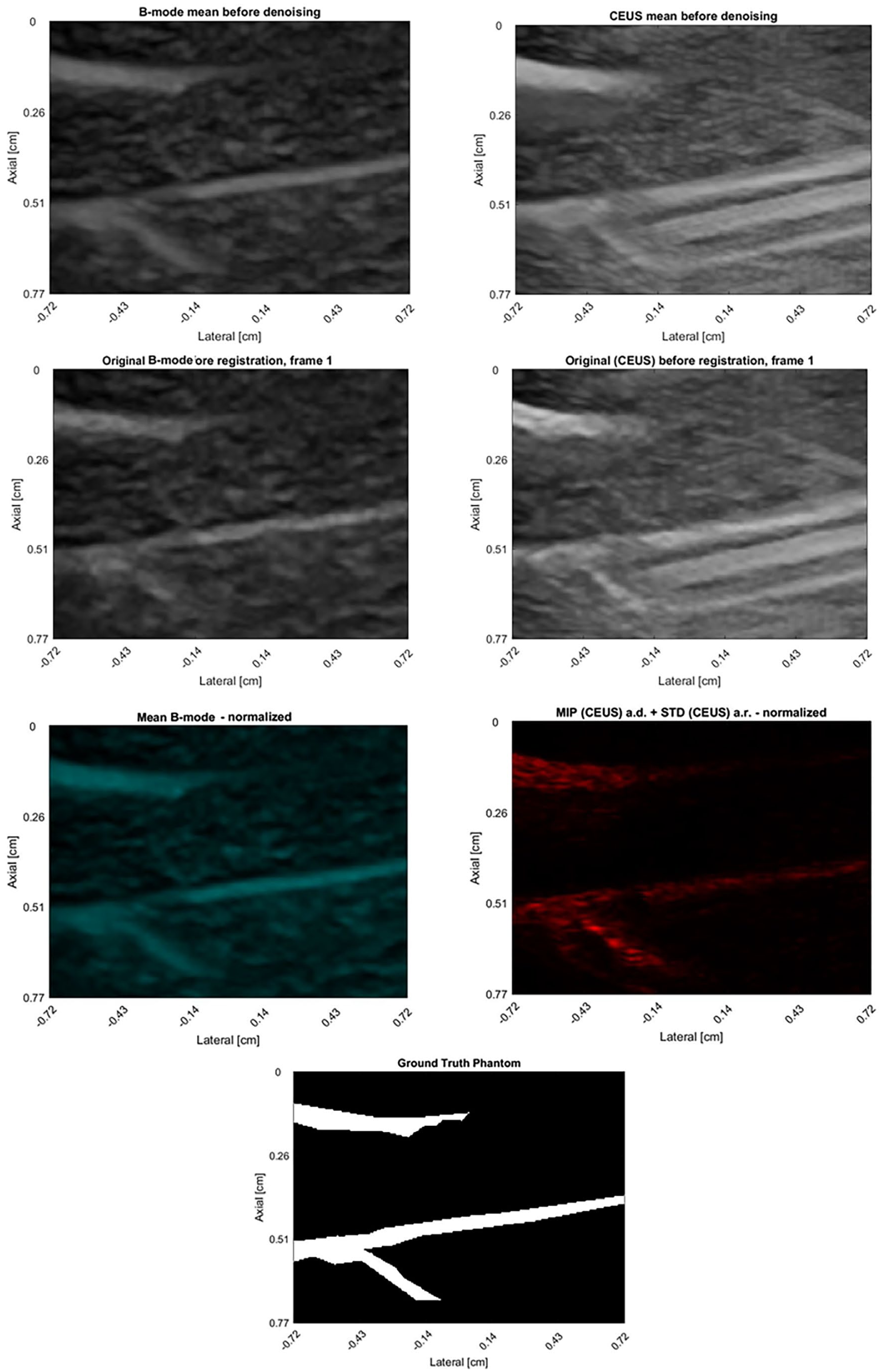
Top left: B-mode image of the phantom. Top right: CEUS image of the phantom. Middle-Top left: Denoised B-mode image of the phantom. Middle-Top right: Denoised CEUS image of the phantom. Middle-Bottom left: Structure extraction from the phantom. Middle-Bottom right: Vascularity extraction from the phantom. Bottom: Ground truth labeled vascularity. a.r. = After registration, a.d. = After deconvolution.
Vascularization Is Defined by the Intensity Properties Within the Marked Pixels Mask (5408 White Pixels in the Ground Truth Image) in Different Images.
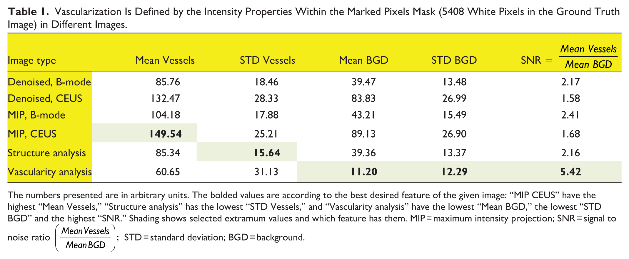
The numbers presented are in arbitrary units. The bolded values are according to the best desired feature of the given image: “MIP CEUS” have the highest “Mean Vessels,” “Structure analysis” has the lowest “STD Vessels,” and “Vascularity analysis” have the lowest “Mean BGD,” the lowest “STD BGD” and the highest “SNR.” Shading shows selected extramum values and which feature has them. MIP = maximum intensity projection; SNR = signal to noise ratio
Pancreas
The patient cohort’s outcomes were categorized into two main groups based on clinical response:
- Unresponsive group: Patients 001, 002, 004 (Figure 8), 006, 007, 010, 011, and 012 exhibited disease progression. Six patients of this group displayed a common characteristic: increased intensity levels, suggesting increased vascularization. Notably, patients 001 and 011 had disease progression but were categorized by the algorithm as having decreased vascularization, while patient 001 was weakly categorized by the algorithm (the sum of slopes:
- Responsive group: Patients 003 (Figure 9), 005, 008, 009, and 013 either underwent surgery or experienced stable PDAC. This group was characterized by decreased intensity levels, indicative of reduced vascularization. Notably, patient 013 had treatment response but was categorized by the algorithm as having increased vascularization, although it was also weakly categorized by the algorithm (the sum of slopes:
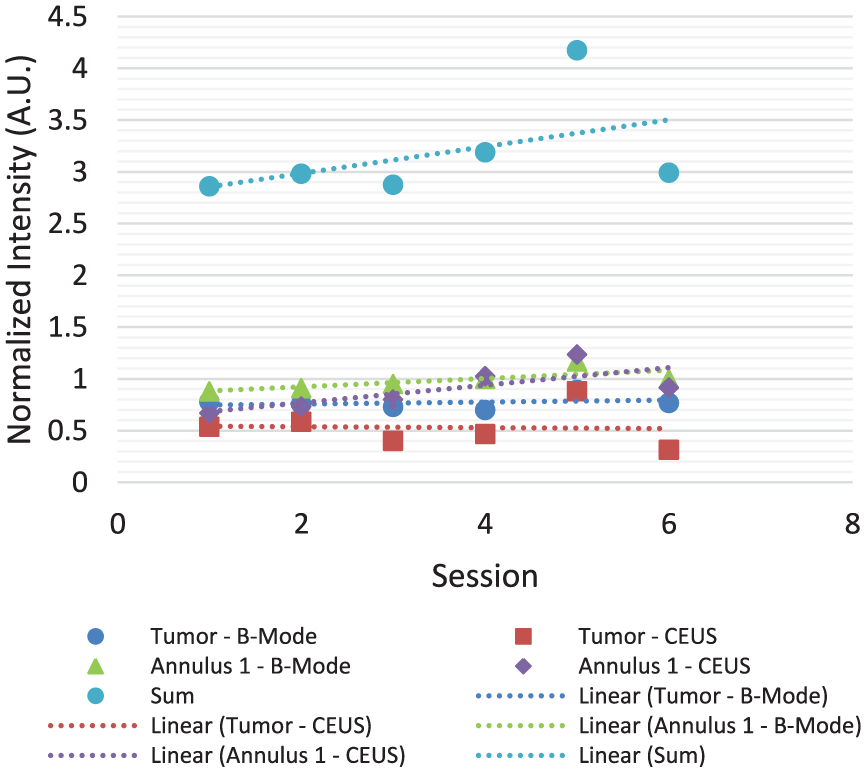
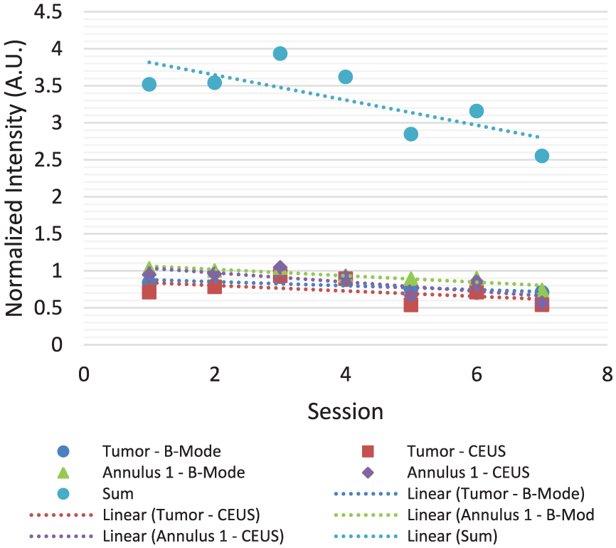
Patient 004. Increasing intensity suggests increased vascularization. Annulus 1—Yellow ring, an index for peripheral vascularity.
Patient 003. Declining intensity suggests decreased vascularization. Annulus 1—Yellow ring, an index for peripheral vascularity.
From the table above (Table 2) one can observe a label fit of 10 out of 13 cases, which represent success rate of 76.9% in predicting the treatment outcomes.
Vascularization Predictions Versus Clinical Outcome Labeling.
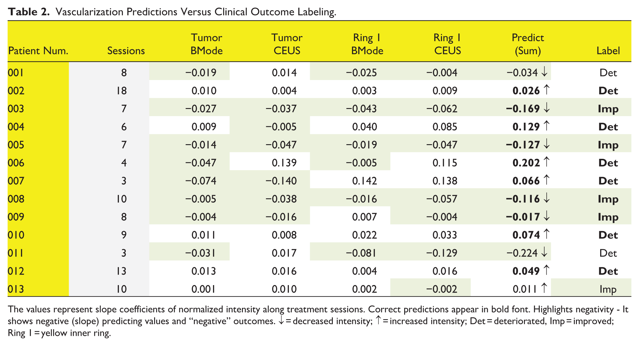
The values represent slope coefficients of normalized intensity along treatment sessions. Correct predictions appear in bold font. Highlights negativity - It shows negative (slope) predicting values and “negative” outcomes. ↓ = decreased intensity; ↑ = increased intensity; Det = deteriorated, Imp = improved; Ring 1 = yellow inner ring.
Discussion
This study investigated the use of US imaging to assess changes in tumor vasculature during pancreatic cancer treatment with sonoporation. CEUS also allowed visualization of microvasculature around the tumor.23,36
The framework focuses on the quantitative assessment of tumor vascularity and its correlation with therapeutic responses. By integrating advanced image processing techniques and statistical analyses, this approach seeks to provide a more accurate and reproducible method for evaluating tumor microvascular changes. Ultimately, the goal is to enhance the precision of monitoring therapeutic efficacy, thereby facilitating personalized treatment strategies and improving patient outcomes in pancreatic cancer.
The mechanics of the drugs used in this study are as follows 37 : FOLFIRINOX—a combination therapy including leucovorin (FOL), 5-fluorouracil (5-FU, F), irinotecan (IRIN), and oxaliplatin (OX), Gemcitabine/Abraxane/Nanoparticle Albumin–bound Paclitaxel (Nab-Paclitaxel)—a commonly used chemotherapeutic drug, composed of paclitaxel bound to albumin.
These mechanisms sabotage the forming of new cancer cells and thus, indirectly, their vascular supplies are expected to decrease as well. Changes in vascular evolution of the functional tumor vessels were found to be closely associated with tumor regression after anticancer treatment. 38
A key challenge was noise in the US images, as well as lack of vascularity, addressed by wavelet filtering and motion correction techniques, improving the detection of signal from background noise. Following image processing, we identified lesions and analyzed blood vessel behavior using deconvolution and MIP methods. Intensity changes were tracked to quantify perfusion. Nonetheless, the frames selection process lost a significant amount of the data and could have damaged the accuracy of the intensity values.
In direct context, the data analyzed was in a digital imaging and communications in medicine (DICOM) format, which is assumed to be log-compressed by the manufacturer. As we do not have access to the compression protocol and other image manipulation which might have taken place, we handled the data as if it was not modified at all. A more accurate analysis would incorporate handling of the log-compression or the use of raw data (with phase, such as RF or IQ data), or demodified data.
A primary drawback from the iterative deconvolution method is computational complexity, potentially impeding future real-time applications. In this work, there were no real-time demands, and it served us well due to its other mentioned advantages.
A better way to quantify the vasculature might be a dilation of the segmented tumor, instead of elliptic rings, and it should be considered in a follow-up research.
The limited number of patients and recorded treatment sessions limited the possibilities of analysis and therefore dividing them into training and test datasets was unrealistic and inaccurate. Thus, a very basic classification method was chosen, both due to the available opportunities and to avoid overfitting with the labeled results. This affects mainly patients 006, 007 and 011 which had 4, 3 and 3 sessions each, correspondingly. The linear regression in these cases might be doubtful.
The movement of both the patients and the sonographers also affects the results, and its impact proceeds to the registration and segmentation parts of the algorithm. The segmentation is sensitive to changes and should be done under careful supervision. Small deviations can change the overall results.
Nonetheless, analysis of patients’ data revealed correlations between changes in vascularity and treatment response. The method achieved a 76.9% success rate in predicting outcomes, with limitations including the need for manual segmentation and sensitivity to motion artifacts. Future applications include improved visualization of vasculature, treatment monitoring, and using the outcome prediction to modify and personalize the patient care.
Conclusion
This study identified promising correlations between a novel analysis of vascular changes and clinical outcomes in patients receiving sonoporation-enhanced chemotherapy with FOLFIRINOX or Gemcitabine/Abraxane. These findings suggest the potential for predicting treatment success using the described method.
Although these results may be influenced by the specific drugs tested, the methodology, which utilizes CEUS imaging holds promise for application with other chemotherapeutic regimens. Further validation in larger patient populations is essential. This approach, with further development, could offer a valuable tool for identifying ineffective treatments early, potentially improving patient outcomes and personalized therapy strategies.
Footnotes
Acknowledgements
I would like to thank Prof. Dan Adam for taking me under his supervision, and for his guidance and suggestions along the research. His ideas helped me broaden my mindset and my professional knowledge, and I am grateful for the opportunity I have been given. And I would like to thank my family, my colleagues and my friends who supported me along the way.
Declaration of Conflicting Interests
The authors declared no potential conflicts of interest with respect to the research, authorship, and/or publication of this article.
Funding
The authors disclosed receipt of the following financial support for the research, authorship, and/or publication of this article: The generous financial help of the National Institutes of Health (NIH, Grant R01CA199646) and the Technion Jacobs graduate school is gratefully acknowledged.