Sage Journals: Discover world-class research

Abstract

Why do some places prosper while others do not? Measuring community-level prosperity is of widespread academic concern and public interest. While quality of life research on urban places is well established, insights into the prosperity of rural places are less developed. Further, much of the rural-oriented literature focuses on economic growth, which has the potential to mask non-growth prosperity characteristics. We follow Isserman et al. (2009) in their efforts to measure community-level prosperity outside the growth-paradigm for U.S. counties. We use geographic sequence analysis to build on their “prosperity index” by extending it longitudinally to measure prosperity at four (approximated) points in time (1990, 2000, 2008–2012, 2018–2022). Sequence analysis allows us to organize multivariate, longitudinal data into prosperity sequence sets – what we term “prosperity pathways” – thus highlighting the importance of time and history into a spatially-informed analysis of prosperity. Our findings enable us to confirm what is ostensibly true in that prosperity is a dynamic and evolutionary process with significant geographic variation.

Keywords

sequence analysis place prosperity community well-being quality of life community development

Introduction

Why do some places prosper while others struggle? Measuring community-level prosperity is of widespread academic and public interest, but the available research on this front largely focuses on urban places, leaving a dearth of research on rural places. Further, much of the rural-oriented literature focuses solely on economic growth indicators such as population, employment, income, and business formation, which has the potential to mask non-growth prosperity evident in many, especially rural, places. To provide insights into the question of place prosperity, Isserman et al. (2009) created a straightforward prosperity index. In this study, we longitudinally extend the Isserman, Feser, and Warren Prosperity Index (hereafter, the “IFW Index”) and evaluate the “path of prosperity” for counties using sequence analysis – an analytical tool to identify, illustrate, and analyze categorical patterns especially in longitudinal data (Losacker and Kuebart 2024). We expand more on this relatively new method in a later section (Data and Methods).

There are significant challenges in defining and measuring place prosperity. First, the literature is rife with alternative measures and definitions making it difficult to identify the outcome of “prosperity.” Indeed, as noted by both Veréb et al. (2024), in a review of the rural focused literature, and Dsouza et al. (2023) in a complementary review of the literature with an urban focus, the literature overall is challenged by the lack of common terminology with some authors talking in terms of well-being or wellness, others vitality, and still more use quality of life or social welfare.¹ Further, most analyses are cross-sectional, treating prosperity as a status rather than a dynamic process. In doing so, there is limited knowledge of changes in prosperity and the factors that drive it, both of which are key to informing policy aimed at place improvement.

With our analysis, we utilize an established definition of prosperity (i.e., the IFW Index), analyze the full breadth of U.S. counties with an intentional consideration of places across the urban-rural spectrum, and consider prosperity over time to better understand the temporal evolution of prosperous places. First, we summarize the IFW Index across four intercensal periods (1990, 2000, ACS 2008–2012, ACS 2018–2022). Then, using sequence analysis, we analyze what we term “prosperity pathways,” which are the resulting sequences of prosperity scores over the study period. We create a novel typology – what we call the “Prosperity Pathway Typology” – to illustrate and categorically interpret prosperity pathway types. We then evaluate the Prosperity Pathway Typology using subsample equivalency testing across a wide range of measures of community prosperity (or well-being or quality of life), which allows us to cross-validate the pathway index to other indicators commonly used in place prosperity literature.

This study advances place-based prosperity literature through four novel contributions, largely through our application of sequence analysis. First, our study offers a comprehensive (rural and urban) analysis of prosperity. Second, we approach prosperity as a dynamic process by extending the analysis over time. Third, we apply sequence analysis to place, rather than individuals – an emerging advancement in sequence analysis methods. Fourth, we create a “Prosperity Pathway Typology” that maintains the uniqueness of place while organizing prosperity pathway types. Ultimately, we demonstrate the heterogeneity of place prosperity and suggest a way forward in making sense of these multiple routes to “prosperity.” Though sequence analysis is a relatively new method, especially for economic geography, we aim through this study to demonstrate its broad utility.

Measuring Prosperity

Understanding place prosperity and the challenges it entails is an important area for research as it has implications for policy agendas and funding allocations, as well as household-level decision making on matters such as family and/or business relocation or personal/business investment. In particular, the well-being of smaller and more rural places, which is less understood, is important for both rural places themselves and for the places that rely on them. As articulated by Green and Zinda (2014), struggles of rural places often have consequences reaching far beyond the bounds of rurality, in part because of the deep reliance of urban places on rural places. Within the context of central place theory, there is a clear interdependency among places of different sizes (Mulligan 1984; Mulligan et al. 2012). In the simplest sense, larger more urban central places offer specialized goods and services to smaller surrounding areas, while smaller more rural places support larger ones by providing a nearby customer base. Beyond commercial ties, the socioeconomic difficulties of rural places matter for the prosperity of all places, from, for example, the security of national food supply to the well-being of the natural environment. Social, economic, and environmental justice issues do not grow any less significant as population density decreases.

Extensive research has sought to measure prosperity and a number of sometimes-synonymous and adjacent concepts such as community well-being (Deller and Parr 2021; Francois et al. 2024; Park and Deller 2021; Schmidt et al. 2024; Veréb et al. 2024), vitality (Etuk and Acock 2017), livability (Dsouza et al. 2023; Kashef 2016; Okulicz-Kozaryn 2013; Wei et al. 2023), and quality of life (Dissart and Deller 2000; Messer and Dillman 2011). Dsouza and her colleagues (2023, 1), however, have found, “minimal consensus across studies on the conceptualization” of quality-of-life, livability or well-being. Substantial variation across terms and how concepts are mobilized for research have led to an inconsistent definition and measurement of “prosperity.” As most recently noted by Veréb and colleagues (2024, 1), the resulting measures are for the most part incompatible with one another, producing a literature that comes across as, “highly fragmented, even contradictory.” In an empirical example of this so-called “chaos”, Etuk and Acock (2017) create and evaluate a prosperity index using factor analysis. They find while their index captures many dimensions of community, it does not successfully measure an underlying concept of community vitality, or prosperity. Though there is no shortage of studies on place prosperity, the lack of consistency in defining prosperity leaves a glaring challenge to the literature.

This lack of definitional consistency is perhaps rooted in the heterogeneity of how different people think about well-being and quality of life: what makes one place’s quality of life higher relative to another place is in the eye of the beholder, begging the question “prosperity for whom?” (Kashef 2016). Some people place high value on access to a variety of cultural venues and events (e.g., museums, theaters, concerts, arts fairs, etc.) while other people place high value on outdoor recreational opportunities and natural amenities. These tastes and preferences also vary across space and over time (Booi and Boterman 2020; Fuguitt and Brown 1990). This heterogeneity is reflected in the literature through “researcher bias” or “observer bias” where a researcher’s personal beliefs, expectations, or assumptions can unintentionally influence the research design (i.e., selection of well-being or quality of life measures) or interpretations of a study.

As another challenge, in many contexts prosperity has been treated synonymously with growth. Growth is a convenient metric as places can be easily compared by how fast their economies grow, how many new jobs they create, how many new houses they build, or how many new people they attract. Indeed, the challenges associated with defining and quantifying prosperity (or well-being or quality of life) are a likely reason that rural development scholars, and economists in particular, have tended to focus on traditional notions of growth. By focusing on growth, researchers bypass the difficulties inherent in defining and measuring well-being or quality of life.

While growth and prosperity are intertwining concepts, they are distinct. That is, growth and prosperity should be considered as separate, but mutually informative, concepts. Conflating growth and prosperity can yield misleading interpretations, especially for rural places, in at least two ways. First, successful rural places often grow and are reclassified as urban places. This produces a narrative that rural places are perpetually left behind. This point was evangelized by Isserman (2001, 2005) and has since been acknowledged for some time (Artz et al. 2005; Coburn et al.2007; Deller and Conroy 2022; Waldorf 2007). In fact, nearly a century before Isserman made his critique, Galpin (1915) discussed the same phenomenon in his early study of a rural Wisconsin county.

Second, many rural places are not growing, nor are they declining, and from a narrow growth perspective, they appear stagnant. This stability, however, is recognized by many as a key contributor to their prosperity. For example, Monroe, Wisconsin in Green County has maintained stable agricultural and recreation-based industries as well as a population of around 10,000 with little deviation (±400) for at least the last 30 years. Despite, or maybe because of this observed stagnation, Monroe is still seen by and large as a “good place to live” and has a vibrant business community. This is a familiar story of many rural places, where those with local knowledge firmly believe these places to be doing well, even though the economy statistically appears stagnant and the population unchanged. Equally as familiar are stories of places inundated with growth, and subsequently struggling. For example, the population of Bozeman, Montana, has nearly tripled in the last 30 years. Infrastructure development and commercial investment are booming. By measures of growth, Bozeman could be called a success story, even prosperous. Severe housing shortages and inadequate social services, however, have left some feeling as if the well-being or quality of life in Bozeman has deteriorated (e.g., Browning and Johns 2024; Shelly 2023). By narrowly focusing on growth (more people, more jobs, more businesses, etc.) as the sole metric of place-based success, we mark these two sorts of places as less-than: a conclusion that can be experientially false and thus an insufficient measure of prosperity.

Disentangling the measurement of prosperity from growth exposes the ways communities across the urban-rural continuum are not homogenous, and nor are their experiences of prosperity. A mountainous college town’s prosperity is not the same as the prosperity of a major urban region. A great deal of effort in place prosperity research revolves around questions of what to include in prosperity measurement that captures the diversity of local experiences. Who’s to say unemployment, for example, is a key indicator of prosperity over crime, or health, or the environment? Why one set of indicators and not others? Should the set of indicators be limited or more extensive? The answers may depend on the community being evaluated. Such “modeling uncertainty” is a consistent challenge in economics (Schmidt et al. 2024), but this challenge becomes especially critical in the interdisciplinary study of place prosperity due to the applied nature of the endeavor.

Empirical studies are increasingly attentive to the multifaceted nature of place prosperity. This includes considering how elements vital to prosperity, such as poverty, vary by both time and place (Curtis et al. 2019). Continuing to explore prosperity from a spatiotemporal lens is an area of critical importance to produce a more encompassing picture of prosperity, especially along the urban-rural continuum. For example, in a recent study analyzing the geographic and temporal distribution of rural livability in China, Wei, Wang, and Fahad (2023) find higher degrees of spatial clustering of their rural livability index over time. That is, space becomes an increasingly relevant feature of livability, but the way it changes is spatially dependent. Put another way, place prosperity research is beginning to highlight how a place is not simply “prosperous” or not, but rather moves in and out of states of more or less prosperity.

In this study, we longitudinally extend and develop the Isserman, Feser, and Warren Prosperity Index – a well-received (e.g., Khatiwada 2014; Rahe 2009; Wilson and Rahe 2016) ordinal prosperity index designed with a rural focus. While we do not herald the IFW Index as the most preferred measure of prosperity, we draw on this Index over others because of its significant advancement in many of the challenges facing place prosperity scholarship, especially in its demonstration of how growth-oriented and urban-centric approaches mask the prosperity of rural places. However, our approach critiques the IFW cross-sectional approach and joins the growing literature calling for more longitudinal and spatial assessments of prosperity (e.g., Kashef 2016). Like Wei and colleagues (2023) among others, we aim to take a spatiotemporal approach to the study of rural prosperity.

The Isserman, Feser, and Warren Prosperity Index

The Isserman et al. (2009) Prosperity Index (IFW Index) is calculated by the composite “score” of four county-level indicators: the poverty rate, the unemployment rate, the high school dropout rate, and a substandard housing measure. The IFW Index is the sum of each of the indicator’s prosperity scores, with an index range of 0 (not meeting any of the prosperity indicators’ criteria) to 4 (meeting all indicators’ criteria).

The poverty rate is the percentage of the county’s population that has a household income at or below the national poverty line. If the county’s poverty rate is below the national average poverty rate, then the county meets the poverty indicator’s criterion for prosperity. For example, if the national average poverty rate is 10 percent but a county’s poverty rate is 8 percent, the county would score a “1” for this prosperity indicator. If the county’s poverty rate is 12 percent, the county would score a “0”. The unemployment rate is similarly measured. The unemployment rate is determined as the percentage of the working population that is not working but seeking employment. If the county’s average unemployment rate is lower than the national average, then the county meets the criterion for prosperity for this indicator. The high school dropout rate is measured as the percentage of 16- to 19-year-olds who are not enrolled in school nor graduated from high school. The same prosperity measurement is used: a below-average dropout rate is a score of “1” for this indicator’s prosperity score.

The housing problems indicator is a Census created county-level indicator of substandard housing conditions. It is composed of four sub-indicators: the percentage of the housing stock (1) without plumbing facilities, (2) without full kitchen facilities, (3) with a high occupancy rate (>1.01 persons per room), and (4) with owner costs or rent exceeding 30 percent of household income. If a county exceeds the national average for any of these four sub-indicators, it does not meet the criterion for prosperity for the housing problems indicator. That is, to meet the prosperity criterion, a county must have a below average amount of housing stock without plumbing or kitchen facilities, a below average rate of households with high occupancy, and a below average percent of households paying more than 30 percent of their income on housing costs.

The IFW Index has served as a foundation for ongoing studies of (rural) prosperity. Subsequent studies have replicated, extended, and employed the Index in distinct ways. For example, in an early adoption of the IFW Index, Rahe (2009) uses the four indicators of prosperity to identify counties that consistently achieve above average outcomes since 1980. This study is aligned with our own study’s objectives of identifying prosperity pathways and profiling cases to learn for purposes of intervention. Khatiwada (2014) uses the IFW Index to explore spatial patterns in prosperity. This is a replication of the Isserman et al. (2009) study but scores prosperity using principal component analysis instead of composite scoring and employs spatial modeling to assess heterogeneity in prosperity. Wilson and Rahe (2016) replicate and longitudinally extend the IFW Index using 2000 decennial Census data and 2008–2012 5-year American Community Survey (ACS) estimates to approximate 2010. They use these data to first identify counties that remained prosperous (score of 4) in the 10-year period and then measure county prosperity level against federal expenditures. They find prosperous rural non-core counties are associated with higher rates of federal expenditures; this finding exhibits spatial dependence within the county level data when using a spatial lag model regressing on federal expenditures. This study also explores the stability of the IFW Index post-recession. They find that overall prosperity declines, but rural prosperity grows. While our study is distinct from these prior replication and extension studies, the consistency in findings across scholars is encouraging in supporting the continued use of the IFW Index as a method for assessing prosperity.

Data & Methods

We expand the cross-sectional IFW Index to a longitudinal approach using US Census data. We use decennial Census data for 1990 and 2000, and American Community Survey (ACS) 5-year estimates (2008–2012 and 2018–2022) to approximate years ∼2010 and ∼2020. While some caution must be extended when comparing decennial and ACS Census data, for longitudinal studies of this time period, blending the two is necessary to capture relevant survey questions. While using 1-year estimates may have been a better match to decennial years, we use the 5-year ACS estimates to more adequately include rural and small counties omitted in the 1-year estimates. This decision is consistent with prior replication studies of the IFW Index (Wilson and Rahe 2016). Our decision to use 1990 as the starting Census period for analysis was motivated in part by data consistency, especially for the substandard housing indicator, as well as to capture the significant changes in rural poverty during the 1990s (Jolliffe 2003).

We begin by first replicating the Isserman et al. (2009) findings using 2000 decennial Census county-level data. We then extend this method for 1990, ∼2010, and ∼2020.² Following Isserman et al. (2009), to calculate a prosperity score, we compare the county-level indicator value to the national average. A 0–1 dummy variable is assigned to each county-year indicator value; if the indicator is “better” than the national average, the score is 1, else 0. The prosperity score is the summation of the four indicators (i.e., 0–4).

To improve the interpretability of the longitudinally extended IFW Index, we use sequence analysis combined with clustering techniques. Sequence analysis is a method of encoding categorical pattern structures. In other words, it is a methodological approach used to study sequences of social behaviors, events, or processes. The method developed in the natural sciences for DNA sequencing and was shepherded into the social sciences by Abbott (1995). In the social sciences, sequence analysis is most often applied to life course processes. For example, Klaesson and Wixe (2023) use sequence analysis in their study of pathways immigrants take through the labor market as students, employees, business owners, and outside of the labor market. An important contribution of our study to sequence analysis literature is the application of sequence analysis to place, rather than to individuals. A recent example of how sequence analysis has been used in this way comes from Connor et al. (2024) in their study of economic mobility of rural children. Like Connor and colleagues (2024), we use sequence analysis to visualize and interpret place-based socioeconomic trajectories.

Sequence analysis is a powerful tool to empirically and visually articulate complex processes over time. In the case of this study, using sequence analysis as a tool to quantify, locate, and interpret prosperity as a process that varies spatially and temporally is significant for future studies of (rural) community well-being and advocates for improved quality of life. Indeed, these objectives align with what Losacker and Kuebart (2024) recently named as the primary objectives of sequence analysis: to “uncover the underlying structure of sequence sets, unveil and cluster typical trajectories, identify prominent characteristics among groups, and examine the interplay between sequences and additional covariates.” Sequence analysis, when combined with clustering, enables us to organize sequence sets into a Prosperity Pathway Typology that straightforwardly visualizes every county, not just the conditional mean as in regression analysis. The method also allows us to “unveil and cluster typical trajectories” of community-level prosperity. In the case of this study, this results in findings that directly confront the narrative of rural decline and presumed value of urbanization.

Performing sequence analysis first involves setting a range of “states.” At each point in time of the sequence analysis, a state is assigned to each observation. In the case of this study, a state is the individual-year prosperity score of a county. That is, states can range from a score of 0–4 for each county-year. The states are then strung together to create a “sequence,” or what we refer to here as an interpretable “Prosperity Pathway.” Each county in the sample has a unique sequence representing the states of prosperity over the study period. One of the principal ways sequence analysis is particularly useful in social science research is by combining it with cluster analysis. We use cluster analysis to group sequences (or pathways) together. This improves the interpretability of findings and visualizes similar sequence groups. By grouping sequences together, researchers can identify typologies in the data that would otherwise be obscured by the sheer quantity or complexity of data.

Findings

The first step in our analysis is to replicate the IFW Index for each temporal point: 1990, 2000, ∼2010, and ∼2020. In 1990, we find 595 counties score as “prosperous” (i.e., 4) on the IFW Index. In 2000, we find 829 prosperous counties. This finding is inconsistent with Isserman et al.’s (2009) findings by 6 counties, but aligns with Wilson and Rahe’s (2016) findings. In ∼2010, we find 743 prosperous counties. This finding diverges from Wilson and Rahe (2016), who find 715 prosperous counties. Their ∼2010 replication, however, does not include Alaska or Hawaii, which may explain some of this variability. In ∼2020, we find 621 prosperous counties. 190 counties remain “prosperous” for the entire study period (Figure 1) – a finding we further explore in later steps. The findings for each of the four individual study years are summarized and spatially shown in Appendix A.

Figure 1.

“Always prosperous” counties; 1990, 2000, ∼2010, ∼2020.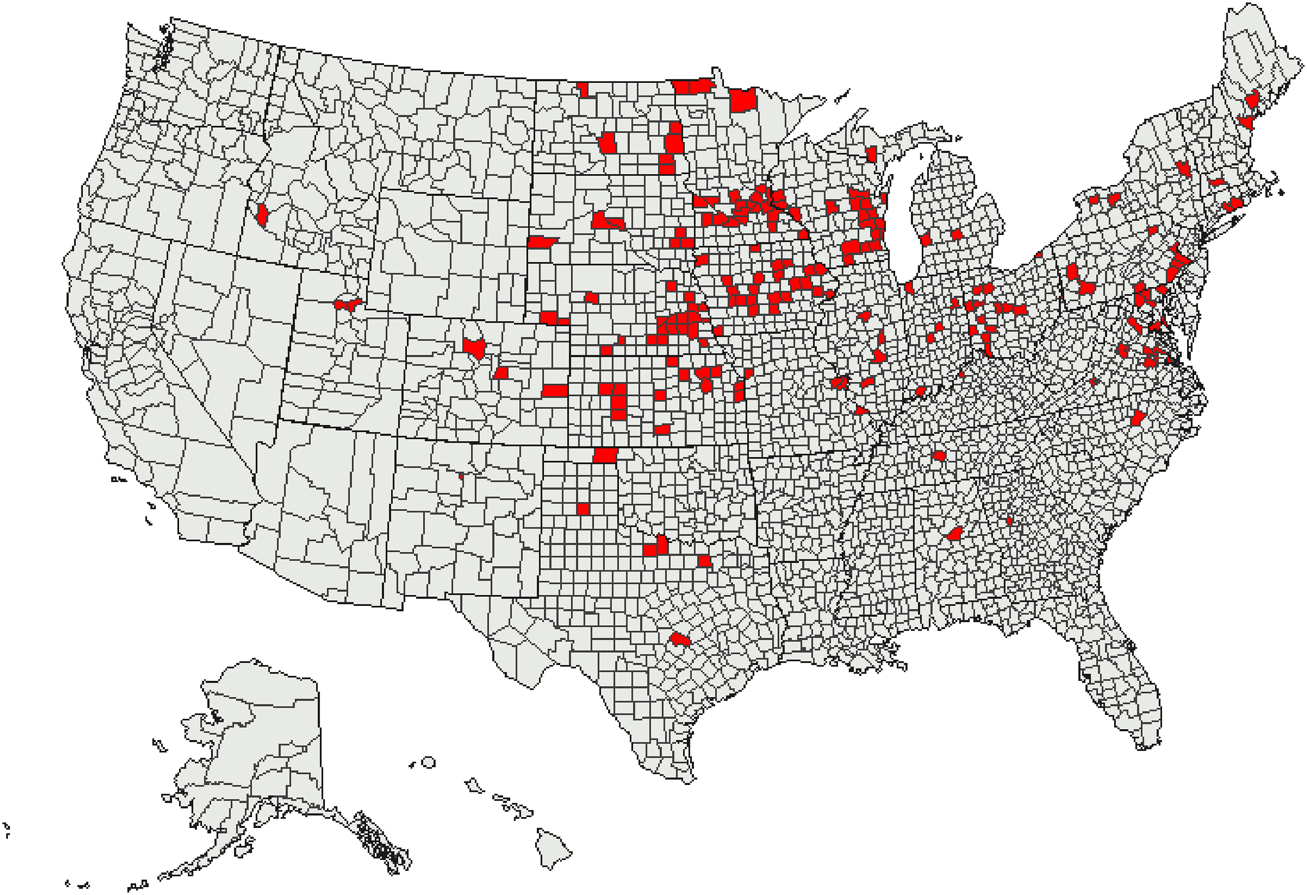

The next step of our analysis strings together the findings of each individual study year to create sequences – what we interpret as “prosperity pathways.” The sequence analysis plot in Figure 2 illustrates the prosperity scores (states) for a random subsample of all counties at each temporal point. The x-axis of a sequence analysis plot represents the data year. The y-axis represents the number of sequences (i.e., pathways). The fill color represents the state, which in the case of our study, is the prosperity score. Each row in a plot corresponds to one county’s sequence. Thus, a county’s prosperity pathway can be visualized by reading across the years for that county’s particular row in the plot.

Figure 2.

Subsample, prosperity pathways (n = 15).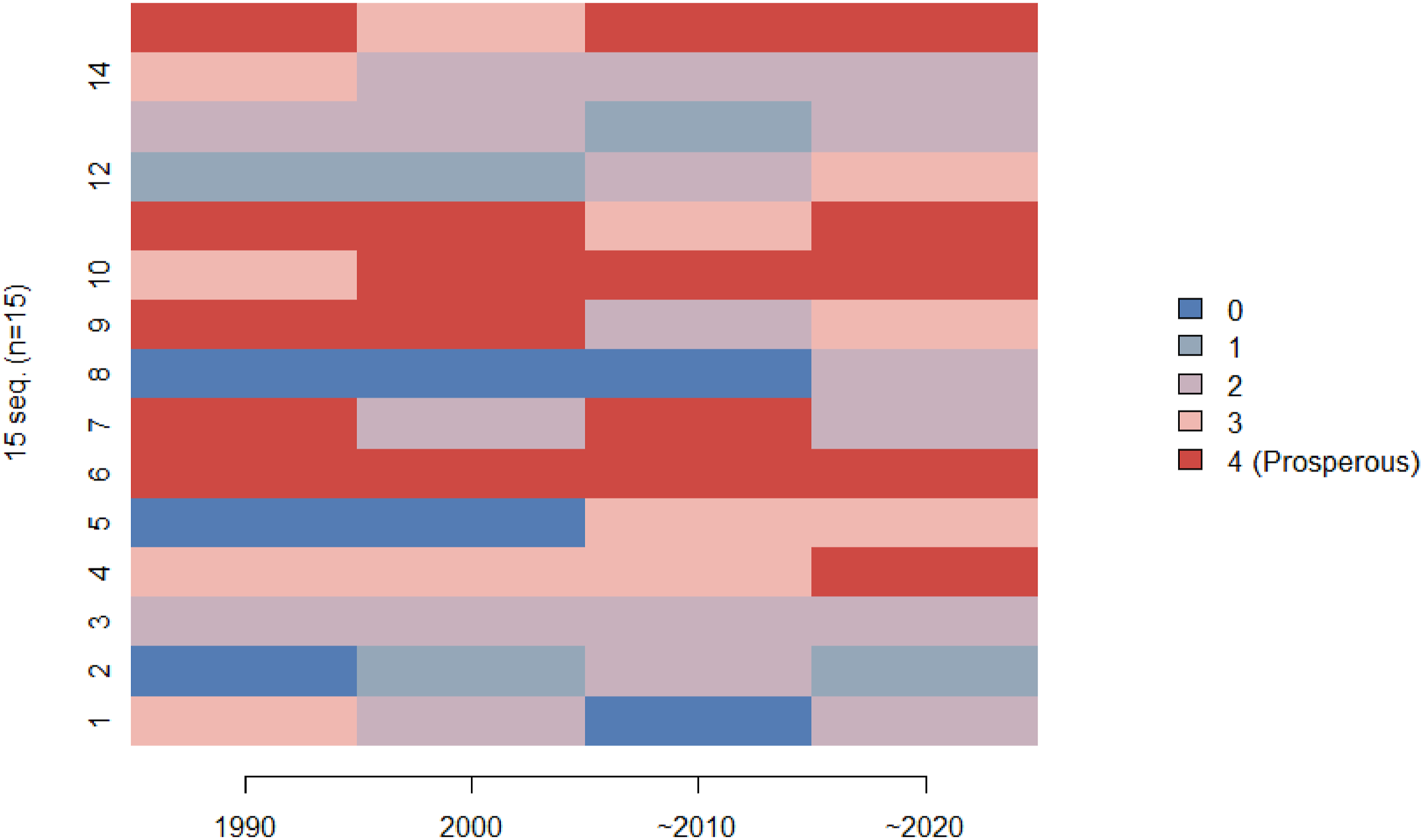

The result is a depiction of prosperity pathways. Again, by pathway, we mean the combination of prosperity scores over the study period. For example, in Figure 2, County 1 scores 3 in 1990, 2 in 2000, 0 in ∼2010, and 2 in ∼2020. This example county’s pathway would then be coded as “3-2-0-2”. County 7’s pathway is “4-2-4-2.”

Through sequence analysis, 313 unique prosperity pathways are revealed. That is, there are more than 300 combinations of prosperity scores over the three-decade period. This finding strongly suggests there is no one way to “achieve” prosperity, nor one way for prosperity to erode. While this finding is to some degree ostensibly true, sequence analysis illuminates in no uncertain terms the breadth of pathways to (and from) prosperity. By way of sequence analysis, we empirically reveal, quantify, and locate prosperity as a dynamic and amorphous place-based characteristic. Such documentation enables discussion of the breadth and variety of Prosperity Pathways beyond casual or broad strokes approximation. Framed from an alternative perspective, however, note that 625 sequences are theoretically possible. Thus, it may come as a surprise, given the data, to only find 313 unique sequences. This suggests there may be some meaningful patterns shaping prosperity pathways. Identifying what those patterns are and how the resulting insights can be translated into policy actions is an important next step for place prosperity research.

More than 300 sequences across more than 3,000 counties make it difficult to identify patterns or trends to assess prosperity. Thus, we use cluster analysis strategies to sort county prosperity pathways into a five-part typology ranging from “lacking measurable prosperity” to “extremely prosperous” (Figure 3). Grouping the sequences into a five-point typology was a conceptually motivated decision based on findings from dendrogram visualization, in reference to the IFW Index scaling, and as an appropriate balance between detail and readability. From a software perspective, we created the typology using the TraMineR RStudio package designed to summarize and analyze categorical sequence data (Gabadinho et al. 2011). The package enables encoding sequence data and the creation of a typology using cluster analysis.

Figure 3.

Typology of prosperity pathways.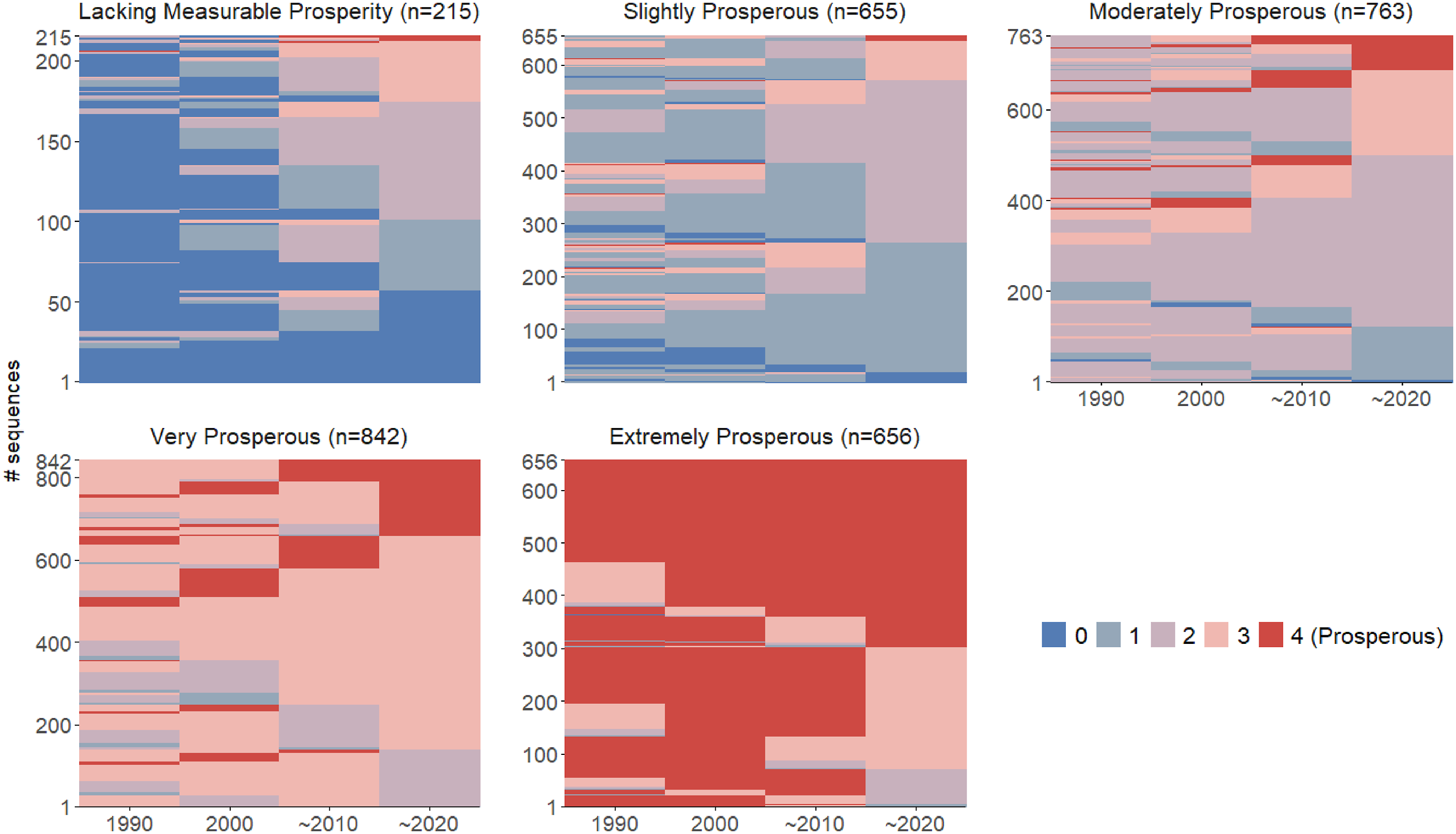

The five groups of the Prosperity Pathway Typology are formed based on pathway similarity, rather than equal size groupings. As a result, the typology is not normally distributed but is skewed: less than seven percent of counties fall into the “lacking measurable prosperity” pathway type, compared to more than 20 percent of counties in the “extremely prosperous” type. Groupings reflect the mode IFW Index score. That is, the five-point scale generally corresponds with the 0–4 indexing, with mostly scores of 0 in the “lacking measurable prosperity” group, mostly 1 in the “slightly prosperous” group, and so on.

Evaluating Prosperity Pathways

While the identified Prosperity Pathway Typology is a helpful first step in understanding notions of prosperity, the Typology in isolation provides little insight into potential policy actions. That is, the Prosperity Pathway Typology mostly follows expectations with few surprises: places with relatively low rates of poverty and unemployment, above average high school graduation rates, and below average substandard housing stock do seem to represent characteristics of prosperity. One way to derive more informative insights from the Typology (and combat the chaos within the quality-of-life literature) is to test its consistency with other prosperity indicators that appear in the literature. To do so, we use subsample equivalency testing. If the Typology is consistent with other commonly used measures this lends support to the robustness of the measure as well as begins laying the foundation for policy insights and literature comparability.

Our central hypothesis is that more prosperous places (proxied by counties) will have better corresponding values of the alternative well-being or quality of life measures. The evidence in support of this hypothesis will come from two steps. First, under the null of no difference in alternative measures of well-being or quality of life across the Prosperity Pathway Typology, significant results from the subsample equivalency indicate the well-being measures do differ across the Prosperity Pathway Typology as expected. Second, given that there is statistical significance in the first step, the means are examined for patterns across the Typology. We expect more prosperous types to correspond to higher (lower) values of the positive (negative) alternative measures. For example, we would expect greater prosperity scores to correlate with higher life expectancy (a positive measure of community well-being) but a lower rate of low-birthweight (a negative measure of community well-being).

The subsample equivalency tests include two tests for central tendency and three nonparametric tests of distribution. The central tendency tests are the ANOVA F-test for mean equivalency and the nonparametric median test of central tendency. The median test categorizes all scores as above or below the median and then tests for differences among the subsamples. The test of median equivalency tests the null hypothesis that the medians of the populations from which the samples are drawn are identical. The median test is considered elementary, but because there are so few assumptions, a statistically significant result is very convincing. The van der Waerden, Savage and Kruskal–Wallis, or Wilcoxon are nonparametric tests that compare the distribution of the measures of community well-being across the subsamples as defined by the Prosperity Pathway Typology. The van der Waerden test is a nonparametric test for the homogeneity of samples based on the rank statistic where the rank scores are the quantiles of a standard normal distribution. The Savage test is similar but is built on an exponential distribution. Kruskai–Wallis is like the Wilcoxon test but is for several subsamples and does not assume a normal distribution.

The alternative measures of well-being include a broad set of local characteristics. Drawing on the existing literature (e.g., Deller and Parr 2021; Etuk and Acock 2017; Francois et al. 2024; Kashef 2016; Messer and Dillman 2011; Okulicz-Kozaryn 2013; Park and Deller 2021; Schmidt et al. 2024; Turkoglu 2015; Wei et al. 2023; Yurui et al. 2020) along with three reviews of this literatures (Dissart and Deller 2000; Dsouza et al. 2023; Veréb et al. 2024), we analyze 21 separate measures grouped into five broad categories including measures of health outcomes, social capital, human capital, economic and population characteristics.

If the analysis reveals the Prosperity Pathway Typology is consistent with the selected alternative measures, this lends a level of confidence in the utility of the Typology and any observable patterns can help inform policy options. This approach is particularly useful given small sample sizes or when we have no priors on the distribution of the data. Subsample equivalency testing, however, cannot infer causation. It can be seen as necessary, but not sufficient, in determining if a variable of interest statistically varies across the Typology. Thus, in one sense, this method lays a minimum threshold for a relationship between our measure and other ideas of well-being and quality of life. In other words, if we fail to find any patterns in the well-being or quality of life measures using this approach, there is likely no relationship to be found using more sophisticated approaches. As such, any insights into policy must be tempered.

The results of the subsample equivalency tests are provided in Table 1. First, across the five categories within the Prosperity Pathway Typology, nearly every indicator shows statistically significant differences across the Prosperity Pathway Typology and varies in the expected way. Only one measure, the density of social advocacy groups within the social capital category, does not appear to vary across the Prosperity Pathway Typology in a statistically meaningful way. Second, looking at the differences in the subsample means, the patterns are consistent across 20 of the 21 measures: the “Extremely Prosperous” group routinely scores “better” than Very-, Moderately-, Slightly-, and Lacking Measurable Prosperity counties. For example, “Extremely Prosperous” counties have higher voter turnout rates and Census participation rates; higher life expectancies, along with lower low-birthweights; and higher educational attainment and performance (i.e., testing) levels. A reasonable conclusion is that our Prosperity Pathway Typology ratings are consistent with alternative measures of well-being or quality of life.

Table 1.

Prosperity pathway typology ratings and broader community characteristics

	Lacking measurable prosperity	Slightly prosperous	Moderately prosperous	Very prosperous	Extremely prosperous	F test	Kruskal-Wallis	Median one-way	Van der Waerden one-way	Savage one-way
Health measures of wellbeing
Average number of physically unhealthy days per month	3.99	3.97	3.72	3.32	2.95	404.73	1139.61	940.52	1073.30	813.01
Average number of physically unhealthy days per month	3.99	3.97	3.72	3.32	2.95	(0.0001)	(0.0001)	(0.0001)	(0.0001)	(0.0001)
Average number of mentally unhealthy days per month	5.04	5.13	5.00	4.66	4.36	199.62	649.90	465.39	631.37	489.54
Average number of mentally unhealthy days per month	5.04	5.13	5.00	4.66	4.36	(0.0001)	(0.0001)	(0.0001)	(0.0001)	(0.0001)
Life expectancy (years)	75.0	75.0	76.3	77.9	78.8	192.26	761.77	622.55	695.47	431.68
Life expectancy (years)	75.0	75.0	76.3	77.9	78.8	(0.0001)	(0.0001)	(0.0001)	(0.0001)	(0.0001)
Percent low birthweight	10.08	9.40	8.41	7.55	6.95	229.32	705.42	615.56	691.74	677.08
Percent low birthweight	10.08	9.40	8.41	7.55	6.95	(0.0001)	(0.0001)	(0.0001)	(0.0001)	(0.0001)
Human capital
Average reading grade performance	2.73	2.87	2.98	3.07	3.17	168.63	542.17	427.01	539.61	382.40
Average reading grade performance	2.73	2.87	2.98	3.07	3.17	(0.0001)	(0.0001)	(0.0001)	(0.0001)	(0.0001)
Average math grade performance	2.69	2.81	2.95	3.06	3.19	191.51	585.63	461.63	594.64	442.35
Average math grade performance	2.69	2.81	2.95	3.06	3.19	(0.0001)	(0.0001)	(0.0001)	(0.0001)	(0.0001)
Percent age 25 and over graduate or professional degree	6.70	6.46	7.30	7.94	9.09	36.42	174.35	118.71	175.56	139.25
Percent age 25 and over graduate or professional degree	6.70	6.46	7.30	7.94	9.09	(0.0001)	(0.0001)	(0.0001)	(0.0001)	(0.0001)
Education index (higher values lower educational attainment)	1.212	1.362	1.320	1.083	0.868	64.81	246.97	195.06	227.25	171.58
	1.212	1.362	1.320	1.083	0.868	(0.0001)	(0.0001)	(0.0001)	(0.0001)	(0.0001)
Social capital
Percent voter turnout	60.40	60.50	63.34	68.06	72.21	180.25	632.10	529.72	591.21	426.01
Percent voter turnout	60.40	60.50	63.34	68.06	72.21	(0.0001)	(0.0001)	(0.0001)	(0.0001)	(0.0001)
Percent census participation	50.87	53.35	56.12	58.54	66.65	155.82	593.96	387.50	601.18	692.60
Percent census participation	50.87	53.35	56.12	58.54	66.65	(0.0001)	(0.0001)	(0.0001)	(0.0001)	(0.0001)
Number of religious congregations per 1K population	2.20	2.49	2.54	2.59	2.09	14.50	71.72	48.41	70.54	48.38
Number of religious congregations per 1K population	2.20	2.49	2.54	2.59	2.09	(0.0001)	(0.0001)	(0.0001)	(0.0001)	(0.0001)
Religious diversity index	0.439	0.487	0.495	0.462	0.415	50.25	207.23	158.98	180.97	172.03
Religious diversity index	0.439	0.487	0.495	0.462	0.415	(0.0001)	(0.0001)	(0.0001)	(0.0001)	(0.0001)
Number of social advocacy organizations per 1K population	0.083	0.061	0.061	0.064	0.065	1.84	12.16	7.98	10.39	7.20
Number of social advocacy organizations per 1K population	0.083	0.061	0.061	0.064	0.065	(0.1186)	(0.0162)	(0.0923)	(0.0344)	(0.1259)
Number of professional organizations per 1K population	0.128	0.141	0.160	0.166	0.191	7.74	72.15	74.78	61.86	60.07
Number of professional organizations per 1K population	0.128	0.141	0.160	0.166	0.191	(0.0001)	(0.0001)	(0.0001)	(0.0001)	(0.0001)
Economic characteristics
Establishment formation rate	0.093	0.088	0.090	0.090	0.084	7.91	33.00	30.22	32.11	35.15
Establishment formation rate	0.093	0.088	0.090	0.090	0.084	(0.0001)	(0.0001)	(0.0001)	(0.0001)	(0.0001)
Establishment churn rate	0.188	0.181	0.180	0.179	0.169	12.86	57.69	32.63	59.98	46.43
Establishment churn rate	0.188	0.181	0.180	0.179	0.169	(0.0001)	(0.0001)	(0.0001)	(0.0001)	(0.0001)
Percent change in population 2000 to 2019	4.53	3.38	7.09	7.26	8.47	5.56	17.85	11.31	22.94	19.16
Percent change in population 2000 to 2019	4.53	3.38	7.09	7.26	8.47	(0.0002)	(0.0013)	(0.0233)	(0.0001)	(0.0007)
Percent change in employment 2000 to 2019	13.03	4.27	9.17	11.65	12.72	5.29	34.84	24.27	36.37	40.26
Percent change in employment 2000 to 2019	13.03	4.27	9.17	11.65	12.72	(0.0003)	(0.0001)	(0.0001)	(0.0001)	(0.0001)
Percent of total Employment in proprietorships	20.78	20.66	21.80	23.05	21.77	19.31	69.04	49.69	69.88	84.54
Percent of total Employment in proprietorships	20.78	20.66	21.80	23.05	21.77	(0.0001)	(0.0001)	(0.0001)	(0.0001)	(0.0001)
Population
Age index (higher values associated with younger populations)	−0.547	−0.668	−0.492	−0.334	−0.531	12.20	51.59	44.95	53.26	40.42
	−0.547	−0.668	−0.492	−0.334	−0.531	(0.0001)	(0.0001)	(0.0001)	(0.0001)	(0.0001)
Median age	37.16	38.99	40.43	41.05	40.97	34.24	150.77	103.31	146.27	81.35
Median age	37.16	38.99	40.43	41.05	40.97	(0.0001)	(0.0001)	(0.0001)	(0.0001)	(0.0001)

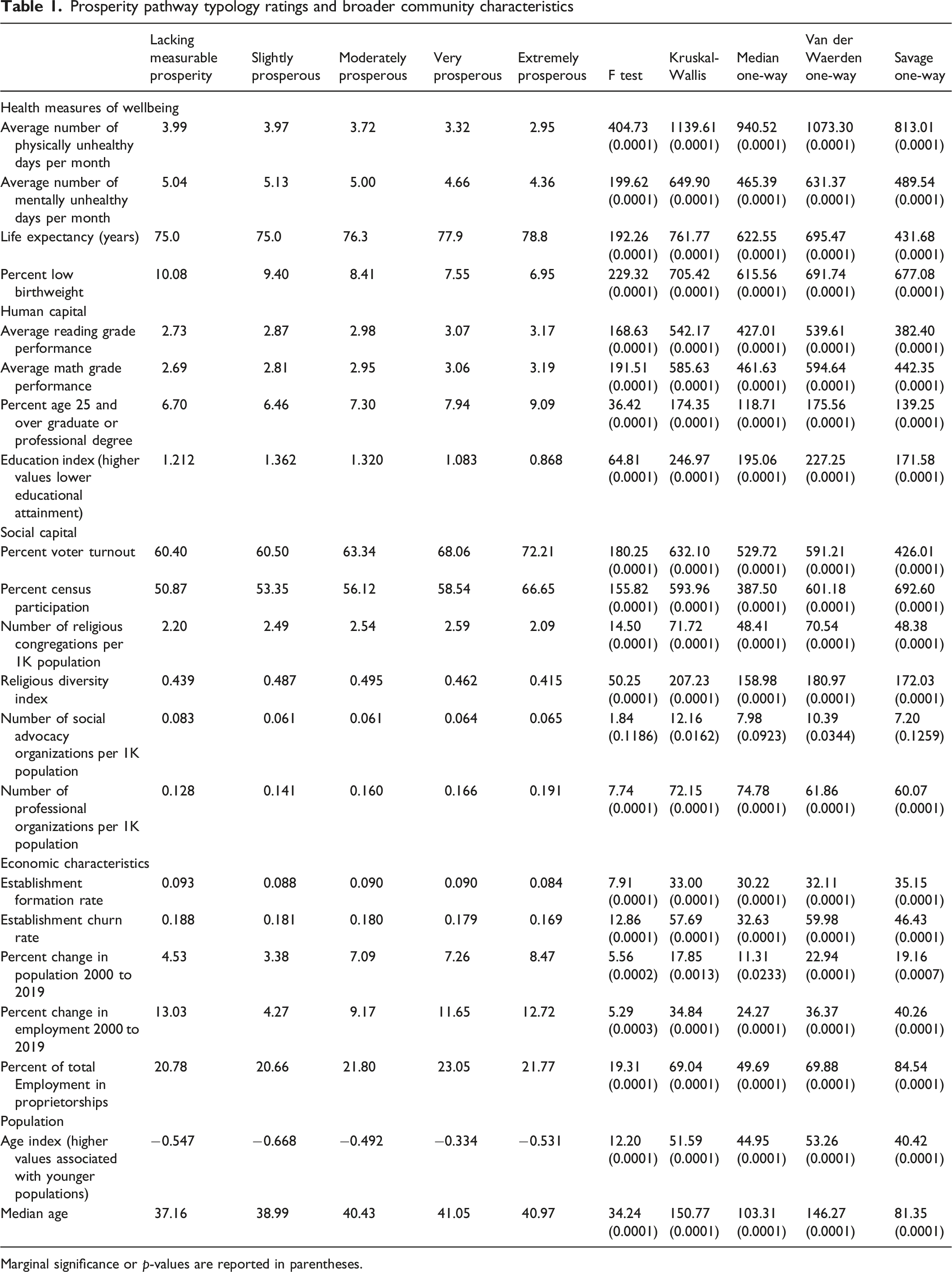
Marginal significance or p-values are reported in parentheses.

Turning attention to the economic characteristic measures, which are designed to proxy more traditional growth measures, the results are more subtle depending on the specific measure. While the statistical tests find that the subsamples across the five prosperity types are different, the pattern across the types is less clear. For example, between 2000 and 2019, both population and employment growth tended to be higher in more prosperous counties. The pattern holds except for counties classified as consistently “Lacking Measurable Prosperity”, which also tended to have slightly higher growth rates. For establishment formation rates, a measure of entrepreneurial activity, it is the highest for counties “Lacking Measurable Prosperity” and the lowest for “Extremely Prosperous” counties. This could reflect differences in entrepreneurship of necessity versus opportunity (Coffman and Sunny 2021). Indeed, it may be the case that counties that consistently score below average for prosperity experience higher rates of entrepreneurship of necessity because of low employment opportunities, whereas “Extremely Prosperous” places provide sufficiently deep employment opportunities to put downward pressure on entrepreneurship of necessity.

The Prosperity Pathway Typology carries promise as a measure of prosperity. For many measures of community well-being or quality of life, the Prosperity Pathway Typology provides results that are consistent with expectations. There are, however, a handful of measures, mostly those associated with different ways of thinking about economic performance, where the results are not consistent with expectations. This limited evidence of inconsistent results between prosperity and economic performance speaks directly to an underlying motivation for this line of prosperity (well-being or quality of life) research: growth and prosperity are not the same. These results suggest that there are places that are growing based on conventional metrics but are not necessarily improving prosperity.

Prosperity Across Geography

With evidence of a robust typology, we proceed with spatial analysis of our measure. To identify spatial patterns within the data we represent the Prosperity Pathway Typology numerically: 0 for “Lacking Measurable Prosperity”, 1 for “Slightly Prosperous”, and so on. A simple mapping of the Prosperity Pathway Typology (Figure 4(a)) and a simple Global Moran’s I (0.445, p < .05) suggest positive spatial dependency within the data; thus, the spatial distribution may not be random. A casual interpretation of the spatial pattern visualized in Figure 4(a) reveals greater prosperity in the Upper Midwest, Great Plains, and New England. Iowa is identified as a particularly “prosperous” state. The Southeast (e.g., the lower half of the Mississippi River region), and Southwest (e.g., southern Texas and the Arizona and New Mexico border region), as well as in parts of the Pacific Northwest, are consistently less prosperous. To further explore these spatial patterns, we conduct both a hot spot analysis, the Getis-Ord Gi* statistic, to identify clusters of similar prosperity types in the Prosperity Pathway Typology (Figure 4(b)) along with a spatial outlier analysis using the Anselin Local Moran’s I statistic to identify places (counties) that are very different compared to their neighbors (Figure 4(c)). We do not include Alaska and Hawaii in these analyses given the importance of spatial contiguity for these tests.

Figure 4.

(a) Map of prosperity pathway typology, (b) Spatial clustering of prosperity pathway typology, (c) Oultlier analysis of prosperity pathway typology.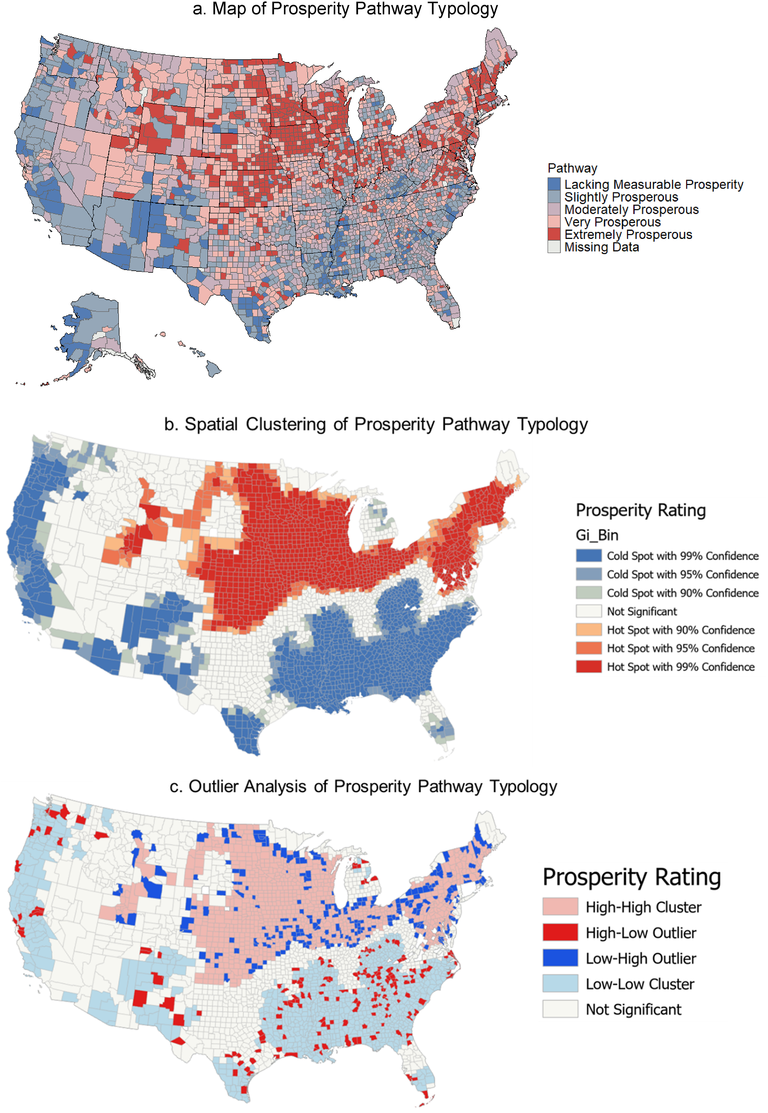

The casual observations drawn from Figure 4(a) are largely confirmed through the Getis-Ord Gi* statistic (Figure 4(b)): much of the region historically associated with the “Rust Belt” through the northern portions of the Great Plains is associated with greater prosperity as defined by Prosperity Pathway Typology. There are three larger geographic clusters of counties that can be characterized as less prosperous: much of the Deep South including parts of eastern Kentucky, parts of West Virginia, and much of western Tennessee; some of the Southwest including much of New Mexico and eastern Arizona; and a broad swath of the Pacific coast. There are also smaller geographic pockets of low prosperity such as the southern tip of Texas, parts of southern Florida, and parts of northeastern Michigan.

The spatial outlier analysis provided in Figure 4(c) largely complements the patterns identified by the Getis-Ord Gi* statistic, but the presence of outliers provides additional insights. Here we can see several counties in the Deep South that are identified as prosperous but are surrounded by low-prosperity counties. Consider, for example, Kenedy County in southern Texas (“Very Prosperous” Prosperity Pathway Type) is surrounded by counties with low prosperity values. Kenedy County is an extremely rural county. With a population of 350, it is the third-least populous county in Texas and fourth-least populous in the United States. At the same time, in many of the larger regions identified as high prosperity, there are counties categorized as less prosperous. A common pattern is prosperous suburban counties surrounded by less prosperous urban core counties such as Chicago (Cook County, Illinois) and Milwaukee (Milwaukee County, Wisconsin). The existence of these “outlier” places suggests the need for a more nuanced view of place prosperity, one that takes seriously both regional relevance and unique place characteristics.

Prosperity Across the Urban-Rural Continuum

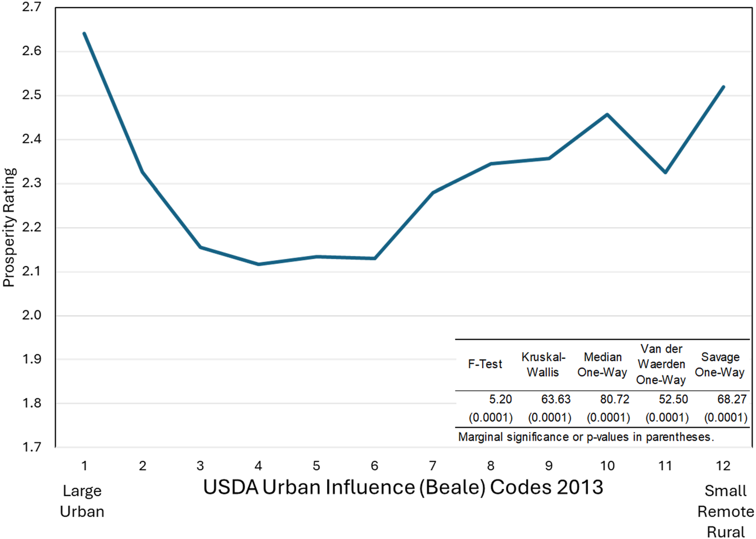
While the overview of the outlier analysis based on the Local Moran’s I is insufficient to draw inferences about differences in prosperity across the urban-rural continuum, there is sufficient prima facie evidence to suggest that such differences exist. To explore differences across the urban-rural spectrum, we group counties using three different systems of rural classification and again apply subsample equivalency testing methods to each.

The first classification system comes from the U.S. Office of Management and Budget (OMB) and classifies counties into three groups. Metropolitan counties are those that are part of a large city and its surrounding suburbs and towns with an urban core population of 50,000 or more, forming an integrated economic and social unit defined by commuting patterns. Micropolitan counties are smaller than a metropolitan area and center around a smaller city or town with an urban core population between 10,000 and 50,000. Nonmetropolitan counties are the remaining relatively rural counties. The second classification is a variation of the first using the traditional metropolitan and nonmetropolitan distinctions, but with nonmetropolitan grouped as either adjacent or nonadjacent to a metropolitan county, with the latter counties being considered remote rural counties. The final grouping uses the U.S. Department of Agriculture’s Urban Influence Codes (UICs), which provide finer classifications of rural counties beyond the simple nonmetropolitan grouping. UICs categorize counties based on their absolute size and proximity to metropolitan areas, micropolitan areas, and access to larger population centers. There are 12 categories ranging from large metropolitan counties with a population of at least one million, to the most rural, which are those not adjacent to a metro or micro area and that do not contain a town of at least 2,500 residents. While the UICs provide a finer level of detail, some care in interpretation is required because they are an ordinal ranking that orders counties based on their relative position or rank; UICs do not provide information about the magnitude of the differences between the class or grouping.

The results for the metropolitan-micropolitan-nonmetro and metropolitan/nonmetro adjacent/nonmetro nonadjacent subsample analysis are provided in Table 2. The observed differences in the subsample distributions are statistically significant. On average, metropolitan counties have the greatest prosperity, followed by nonmetropolitan counties, particularly those that could be considered remote. The subgroupings with the lowest average prosperity are for micropolitan and adjacent nonmetropolitan counties. While these results suggest there are differences in prosperity across the urban-rural divide, these simple three subgroupings do not provide sufficient insights to draw meaningful inference. The subsample equivalency testing using the Urban Influence Codes (UICs) provides a finer insight into urban-rural differences. We map the subsample means in Figure 5, along with the test statistics. Here there is a clear, and significant, U-shaped pattern between prosperity rating and the urban-rural spectrum. Consistent with the two simpler sets of results (Table 2), where the most urban and smallest most rural counties are the most prosperous.

Table 2.

Prosperity pathway typology ratings over the urban-rural divide

	Metropolitan	Micropolitan	Neither metro/ micro	F-test	Kruskal- Wallis	Median one-way	Van der Waerden one-way	Savage one-way
Prosperity Rating	2.442	2.227	2.296	7.56 **(0.0005)	17.36 **(0.0002)	15.16 **(0.0005)	15.32 **(0.0005)	26.04 ***(0.0001)
	Metro	Nonmetro adjacent	Nonmetro remote
Prosperity Rating	2.442	2.156	2.400	16.82 ***(0.0001)	37.03 ***(0.0001)	38.67 ***(0.0001)	31.78 ***(0.0001)	40.54 ***(0.0001)

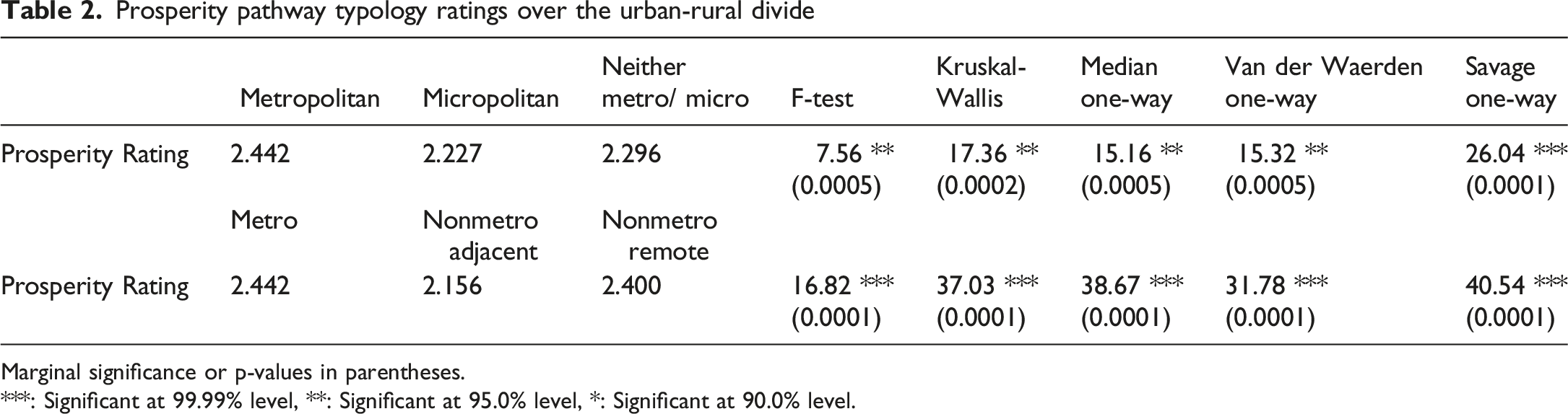
Marginal significance or p-values in parentheses.

***: Significant at 99.99% level, **: Significant at 95.0% level, *: Significant at 90.0% level.

Figure 5.

Prosperity pathway typology rating across the urban-rural divide.

Prosperity Over Time: Stability and Change

Our findings from the Prosperity Pathway Typology suggest prosperity changes over time, is regionally informed, and varies across the urban-rural continuum. One of the main challenges in place prosperity research relates to the dynamic nature of prosperity itself. Places evolve, rendering them more or less prosperous as people move in and out, businesses open and close, and policies come and go. Our Prosperity Pathway Typology addresses this challenge by illuminating the ways prosperity is stable or changing in places over time. This contribution is especially relevant for applied questions around how to create, or maintain, prosperity. Here, we offer three insights into the stability and change of prosperity, as elucidated by the Prosperity Pathway Typology. To emphasize these points, we select several illustrative county examples to serve as “case studies” or “vignettes” (Barkley 2008).

First, when comparing the prosperity types to population growth, our approach reveals how population, and likely other growth measures, offer inadequate depictions of place prosperity. Three counties exemplify this point. Rockingham County, New Hampshire is a straightforward example of a place where population growth and prosperity appear aligned. Rockingham County is a coastal retreat area with significant prosperity improvement – jumping from 2 in 1990 to 4 in 2000 and thereafter. The fourth wealthiest county in New England, Rockingham County is categorized as “extremely prosperous.” The county has had sizable population growth, especially in the latter half of the twentieth century and was the fastest growing New Hampshire county from 2010 to 2020. Thus, it may be tempting to connect this growth to the improving prosperity pathway, telling a story of prosperity rooted in urbanization. On the other hand, Garfield County, Nebraska is less amenity rich and has consistently lost population since 1950 (except for moderate growth in 2010). This county’s prosperity score, however, is also improving from 2 in 1990 to 3 in 2000 to 4 in ∼2010 and ∼2020. This is a “moderately prosperous” county, on an upward trajectory, despite persistent population loss. A resulting narrative from this county suggests population change is not an effective proxy measure for prosperity. As a final example of this point, despite significant and sustained population growth, Cache County, where Utah State University is located, has retained a score of 3 for the study period and is categorized as “very prosperous.” Population growth in this county does not correspond to any change in prosperity. Why the prosperity-population relationship of Rockingham, Garfield, and Cache Counties are experienced differently is left opaque; however, this lack of consistency suggests maintaining a skepticism of using growth as a one-dimensional assessment of prosperity.

Second, we find stability in prosperity within all categories, but stability is characteristically different across places. Around 13 percent of all counties (406 counties) included in the longitudinal sample, never change prosperity score and fall into their respective type group (i.e., 0 for lacking measurable prosperity, 1 for slightly prosperous, etc.). This stability occurs for counties ranging from the most prosperous to the least. For example, Ozaukee County, Wisconsin is in the “extremely prosperous” group and has scored a 4 for each study period year. Ozaukee County is a predominately White high-income suburb north of Milwaukee, one of the most racially segregated cities in the United States (Levine 2020). On the other hand, Fresno County, California has scored a 0 for each study period year and in our study is coded as “lacking measurable prosperity.” Fresno County has a majority Latinx population and is the hub of Central Valley agricultural production. One way our spatiotemporal approach explores the question of why some places prosper while others do not is through identifying the stability of prosperity across time. The finding that explicitly names places like Ozaukee County as stable in its extreme prosperity and Fresno County as stable in its lack of “prosperity” makes it nearly impossible to ignore the influence of historical legacy, such as racial oppression, in understanding place prosperity.

As a clear example of how historical legacy shapes contemporary place prosperity, in our study, Washington County, Mississippi also scores a 0 for all four study period years and is classified as “lacking measurable prosperity.” In 1860, Washington County had the second highest enslaved population in the United States, a fact with considerable modern-day implications, as findings from O’Connell (2012) identify 1860 slave concentration to be directly related to contemporary inequalities. Thus, in addition to shedding light on the stability of prosperity, or lack thereof, there are indications of the pathway typologies aligning with extensive previous research findings around historical processes and contemporary well-being. Though our study does not unpack the reasons for prosperity or lack thereof, the longitudinal approach is telling of the ways prosperity is a spatiotemporal process with lasting implications.

A third insight comes from the diversity of prosperity pathways and the courses of change over time. While some counties in our study demonstrate remarkable stability in prosperity over time, we find other counties, even within a prosperity “type”, experience substantial change in prosperity and the path of change is different across counties. For some places, the change is sudden, with relatively clear cause. One example is Clayton County, Georgia, located just south of Atlanta. In 2008, the Clayton County School District lost its accreditation due to administrative shortcomings surrounding the district school board (Lohr 2008). This corresponds to a drop in prosperity score, from 2 in 1990 and 2000 to 0 in ∼2010 and ∼2020. Although the county changed from a more moderate score to the lowest score, the county is within the “lacking measurable prosperity” category in the Prosperity Pathway Typology. While this is an immediate “shock” event, there are other cases where the change occurs more over time. For example, Maui County, Hawaii made international headlines when devastating wildfires broke out in late summer 2023, but it is likely these effects were exacerbated by climate effects that have led Hawaii to see a more than 30 percent reduction in wet season rainfall since 1990 (Longman et al. 2015). The persistent drought conditions that led to the Maui wildfires are perhaps one part of the narrative for Maui County’s declining prosperity. Maui County is in the “slightly prosperous” category, scoring a 3 in 1990 and 2000, 2 in ∼2010, and 1 in ∼2020. This eroding prosperity is certainly part of the conversation alongside the devastating effects of the 2023 wildfire. Unlike Clayton County, which experienced a policy change that corresponds with an immediate prosperity change, places like Maui County reflect a slower change in prosperity, one more reflective of long-term trajectories of change.

The insights we derive here, by way of these selective examples, demonstrate the utility of sequence analysis in both scholarly and applied settings. First, that population growth is not a reliable barometer for place prosperity can shape future research directions. Improving our understanding of the relationship between population and prosperity is critical for local community economic development, for example in decision-making around where to direct local resources to promote community well-being. Second, the notable stability of prosperity, and the ways that stability may be related to persistent historical context, calls for a more locally informed, regional approach to measuring quality of life. Such an approach stands to equip local practitioners with more nuanced data relevant for their own applications. Finally – and perhaps most encouragingly – we find that prosperity does change. Geography need not be destiny (Isserman et al. 2009, 328). More research is required to understand the nature of these changes – the types, drivers, and consequences of changing prosperity. As noted above, this application of sequence analysis and subsequent analysis of the patterns uncovered ought not be used to make definitive policy recommendations as any notions around causation are not addressed.

Conclusion

To move beyond narrow concepts of economic growth as the only measure of community prosperity, there has been substantial growth in the number of studies on place prosperity, sometimes referred to as well-being, vitality, livability, or quality of life. As might be implied by the breadth of terms used to measure place prosperity, there is an alarming absence of empirical consistency in how researchers think about and measure well-being, especially across disciplinary bounds. Indeed, as described by Veréb et al. (2024), the current state of the literature could best be described as in a state of chaos.

Within this ongoing discourse, we find calls for taking place heterogeneity seriously, deemphasizing growth as a one-dimensional proxy for well-being, and considering prosperity as a process rather than a fixed state. In this study, we take steps to address these concerns by developing one well-received prosperity index. In doing so, we explore opportunities to engage with the noted challenges within this body of research. This includes assessing prosperity across the urban-rural divide and over time as well as conceptually advancing the applications of sequence analysis in ways that aid our efforts to organize prosperity pathways into a typology that retains the uniqueness of places.

The findings from this study demonstrate prosperity is temporally dynamic and spatially relevant. We find more than 300 prosperity pathways, supporting the perspective that there is no universal roadmap to achieving prosperity; however, we maintain there are tangible ways to better understand the relative prosperity of places, the many ways places experience prosperity, and how prosperity changes over time and place. We investigate these possibilities by developing a Prosperity Pathway Typology, which we evaluate through subsample equivalency testing and spatial analysis. Through this evaluation, we find consistency across other measures of prosperity and further evidence to support economic growth is not a reliable proxy to measure prosperity. We find prosperity can be stable over time, but that stability is characteristically different depending on place. While some places are marked by stability, we also find prosperity can and does change – a promising finding for those invested in the betterment of places. However, how and why those places change is an area in need of further exploration.

As we have already noted, there are limitations to the IFW Index approach that carry through to the Prosperity Pathway Typology. The IFW Index, and consequently the Prosperity Pathways Typology, is parsimonious in at least two ways. First, the narrow scope of indicators to measure prosperity largely ignores issues of equality (including by race and gender), health, environmental degradation, and the nexus of these missing components – all of which clearly matter for the lived experience of places. While the broader measures of the IFW Index to some degree capture these matters (e.g., measuring health through poverty), the lack of explicit reckoning with these issues is consequential for how we interpret prosperity findings. Places shape matters of, for example, racial equality, which in turn shape places (Lipsitz 2011). Again, that Fresno County, California is identified as “lacking measurable prosperity” and Ozaukee County, Wisconsin is identified as “extremely prosperous” is no accident, but the mechanisms behind this assessment are obscured by the absence of meaningful measures of structural inequality in these indices.

Second, regional patterning in prosperity is overwhelmingly evident and the IFW Index model includes no spatial controls to address this fact. While we acknowledge, and in fact champion, the notion that prosperity can take many forms, that the Prosperity Pathway Typology and the IFW Index suggest Iowa is consistently more prosperous than places like New York City, Chicago, or Los Angeles raises skepticism. What prosperity is for a major urban center will be decidedly different from what makes a remote rural town prosperous. Although measurements at the county-level are convenient for analysis, this scalar unit may mask important within-county variation and draws concern for earnest nationwide comparability, especially across the urban and rural continuum (Bell 2007). Comparing all counties to a single national average, as these indices do, does not sufficiently take rurality and regional context into account. Instead, comparing to a metro average or a regional average may be more effective in accounting for the way spatial relationships affect prosperity.

Despite the limitations of the IFW Index, and the derived Prosperity Pathway Typology, we find the simplicity of the Index composition advantageous in exploring the conceptual notion of prosperity as a dynamic process over time and space. The four indicators that make up the IFW Index are inarguably relevant to prosperity, albeit incomplete. Places with low poverty, high education rates, plentiful jobs, and good quality housing do in fact seem to be better places to live, at least in some ways. However, what this study demonstrates is that prosperity does not look the same across places. More than 300 prosperity pathways indicate prosperity itself is not a stagnant term. No universal roadmap to prosperity exists. Thus, to measure prosperity, future research must consider how indicators of prosperity may vary over place: what matters for prosperity in one place may not be the same as what matters someplace else.

The policy implications of this line of work are clear: top-down approaches to community betterment are likely to fail as such approaches cannot reflect the diverse ways places think about prosperity. Policies that are extremely effective in some places may fail elsewhere. Grassroots or bottom-up policy initiatives that allow places to define their own notions of prosperity enable the development of policy strategies that leverage the uniqueness of place, including the unique role they play within broader regional economic systems. This is of course not to say higher levels of government at the state and federal levels do not play a role in community betterment initiatives; they are, however, in a supportive role, allowing a place to self-determine what prosperity looks like for itself and how best to enhance quality of life given its individual circumstances. Though there is still a long way to go in this line of research, wading through the chaos to better understand how places thrive remains a worthwhile endeavor for the well-being of those who call these places home.

Footnotes

Acknowledgements

Our thanks to the members of the Rural Livability Lab and the Spatial Thinking Working Group for their helpful comments and support in the shaping of this publication. We are also grateful for the contributions of David Heinritz, Mary McDermott, and Sara Peters.

ORCID iDs

Danielle Schmidt

Tessa Conroy

Funding

The authors disclosed receipt of the following financial support for the research, authorship, and/or publication of this article: Financial support for the research, authorship, and publication of this article comes from the Wisconsin Rural Partnership Initiative at the University of Wisconsin-Madison, part of the USDA-funded Institute for Rural Partnerships (2023-70500-38915) and the United States Department of Commerce Economic Development Administration in support of Economic Development Authority University Center [Award No. ED21CHI3030029].

Declaration of Conflicting Interests

The authors declared no potential conflicts of interest with respect to the research, authorship, and/or publication of this article.

Data Availability Statement

Data is available from the authors upon request.*

Notes

Appendix

Table A1.

1990 IFW index results, by region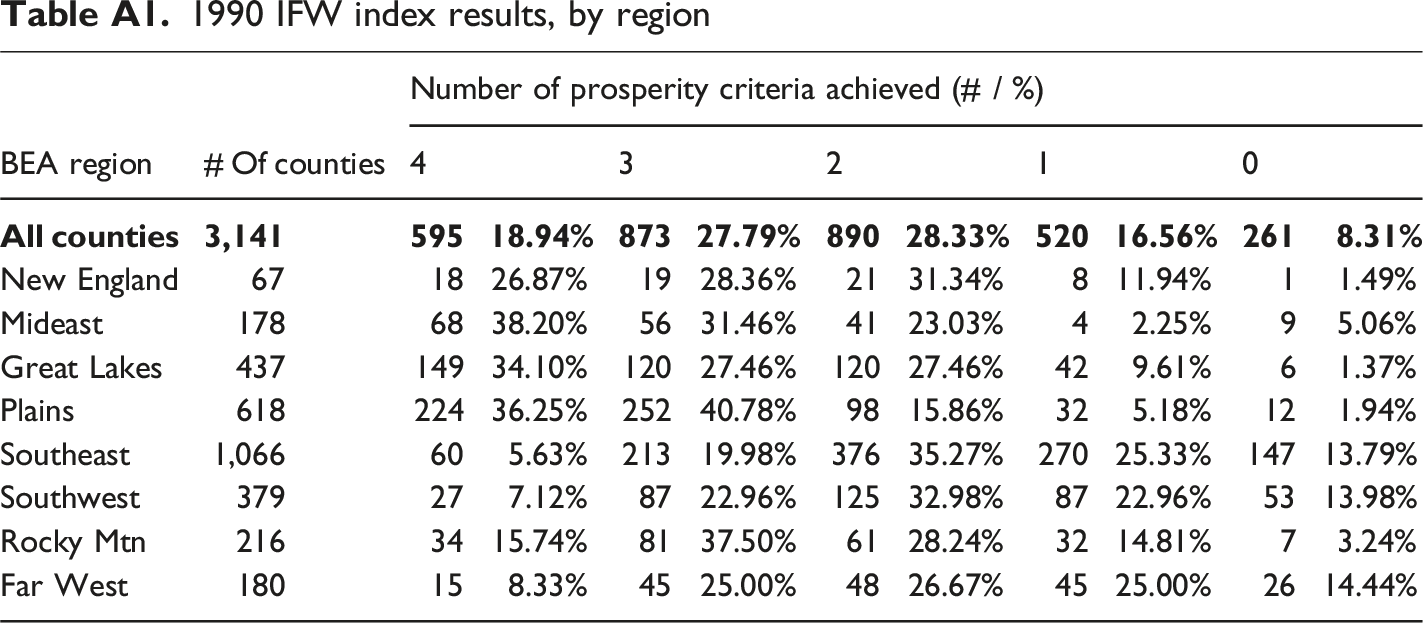

BEA region	# Of counties	Number of prosperity criteria achieved (# / %)
BEA region	# Of counties	4		3		2		1		0
All counties	3,141	595	18.94%	873	27.79%	890	28.33%	520	16.56%	261	8.31%
New England	67	18	26.87%	19	28.36%	21	31.34%	8	11.94%	1	1.49%
Mideast	178	68	38.20%	56	31.46%	41	23.03%	4	2.25%	9	5.06%
Great Lakes	437	149	34.10%	120	27.46%	120	27.46%	42	9.61%	6	1.37%
Plains	618	224	36.25%	252	40.78%	98	15.86%	32	5.18%	12	1.94%
Southeast	1,066	60	5.63%	213	19.98%	376	35.27%	270	25.33%	147	13.79%
Southwest	379	27	7.12%	87	22.96%	125	32.98%	87	22.96%	53	13.98%
Rocky Mtn	216	34	15.74%	81	37.50%	61	28.24%	32	14.81%	7	3.24%
Far West	180	15	8.33%	45	25.00%	48	26.67%	45	25.00%	26	14.44%

Table A2.

2000 IFW index results, by region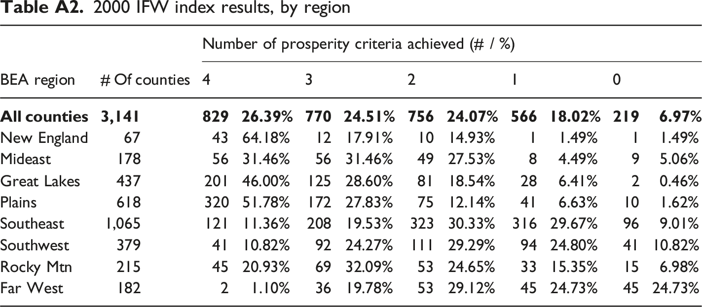

BEA region	# Of counties	Number of prosperity criteria achieved (# / %)
BEA region	# Of counties	4		3		2		1		0
All counties	3,141	829	26.39%	770	24.51%	756	24.07%	566	18.02%	219	6.97%
New England	67	43	64.18%	12	17.91%	10	14.93%	1	1.49%	1	1.49%
Mideast	178	56	31.46%	56	31.46%	49	27.53%	8	4.49%	9	5.06%
Great Lakes	437	201	46.00%	125	28.60%	81	18.54%	28	6.41%	2	0.46%
Plains	618	320	51.78%	172	27.83%	75	12.14%	41	6.63%	10	1.62%
Southeast	1,065	121	11.36%	208	19.53%	323	30.33%	316	29.67%	96	9.01%
Southwest	379	41	10.82%	92	24.27%	111	29.29%	94	24.80%	41	10.82%
Rocky Mtn	215	45	20.93%	69	32.09%	53	24.65%	33	15.35%	15	6.98%
Far West	182	2	1.10%	36	19.78%	53	29.12%	45	24.73%	45	24.73%

Table A3.

∼2010 IFW index results, by region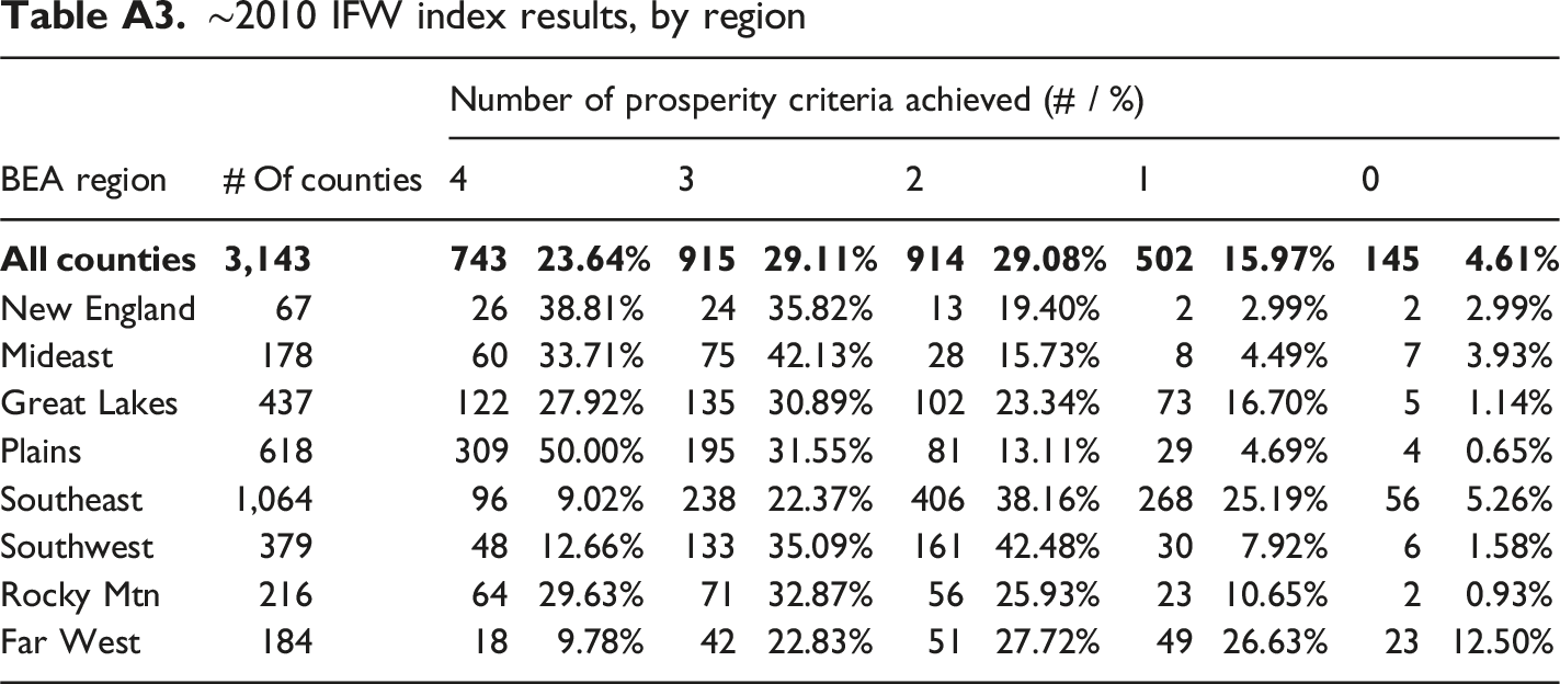

BEA region	# Of counties	Number of prosperity criteria achieved (# / %)
BEA region	# Of counties	4		3		2		1		0
All counties	3,143	743	23.64%	915	29.11%	914	29.08%	502	15.97%	145	4.61%
New England	67	26	38.81%	24	35.82%	13	19.40%	2	2.99%	2	2.99%
Mideast	178	60	33.71%	75	42.13%	28	15.73%	8	4.49%	7	3.93%
Great Lakes	437	122	27.92%	135	30.89%	102	23.34%	73	16.70%	5	1.14%
Plains	618	309	50.00%	195	31.55%	81	13.11%	29	4.69%	4	0.65%
Southeast	1,064	96	9.02%	238	22.37%	406	38.16%	268	25.19%	56	5.26%
Southwest	379	48	12.66%	133	35.09%	161	42.48%	30	7.92%	6	1.58%
Rocky Mtn	216	64	29.63%	71	32.87%	56	25.93%	23	10.65%	2	0.93%
Far West	184	18	9.78%	42	22.83%	51	27.72%	49	26.63%	23	12.50%

Table A4.

∼2020 IFW index results, by region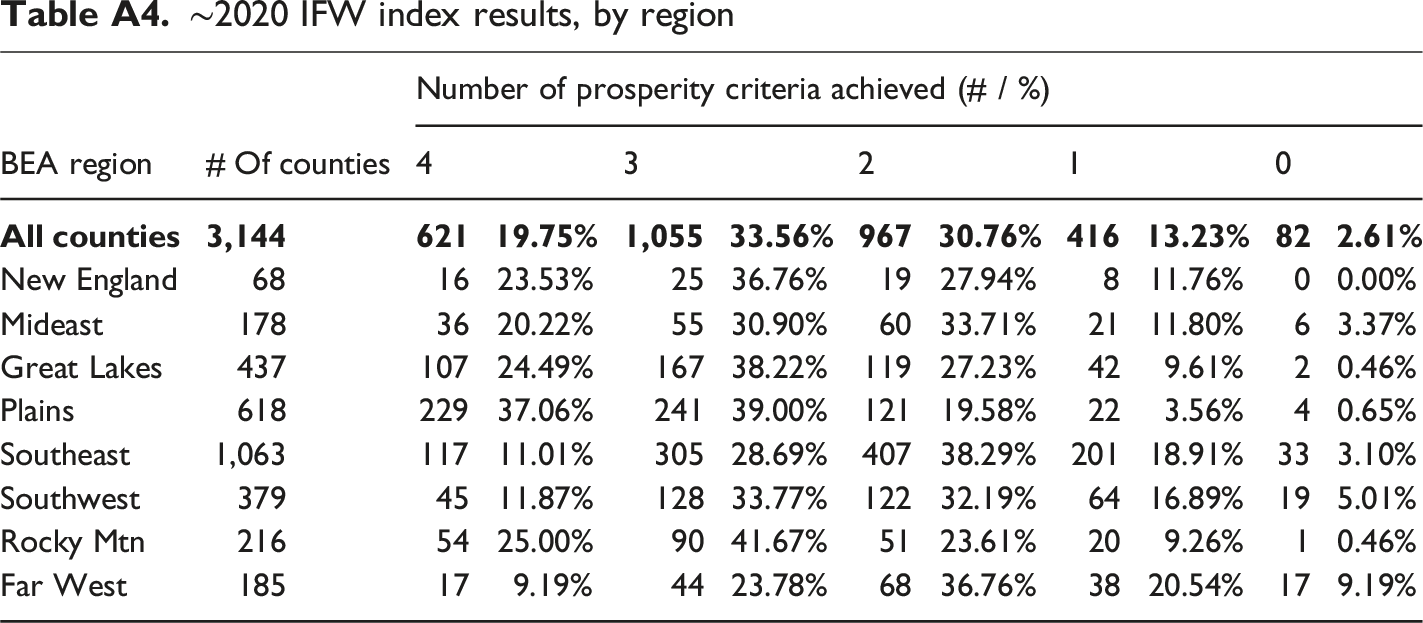

BEA region	# Of counties	Number of prosperity criteria achieved (# / %)
BEA region	# Of counties	4		3		2		1		0
All counties	3,144	621	19.75%	1,055	33.56%	967	30.76%	416	13.23%	82	2.61%
New England	68	16	23.53%	25	36.76%	19	27.94%	8	11.76%	0	0.00%
Mideast	178	36	20.22%	55	30.90%	60	33.71%	21	11.80%	6	3.37%
Great Lakes	437	107	24.49%	167	38.22%	119	27.23%	42	9.61%	2	0.46%
Plains	618	229	37.06%	241	39.00%	121	19.58%	22	3.56%	4	0.65%
Southeast	1,063	117	11.01%	305	28.69%	407	38.29%	201	18.91%	33	3.10%
Southwest	379	45	11.87%	128	33.77%	122	32.19%	64	16.89%	19	5.01%
Rocky Mtn	216	54	25.00%	90	41.67%	51	23.61%	20	9.26%	1	0.46%
Far West	185	17	9.19%	44	23.78%	68	36.76%	38	20.54%	17	9.19%

Figure A1.

County-level map of 1990 IFW index.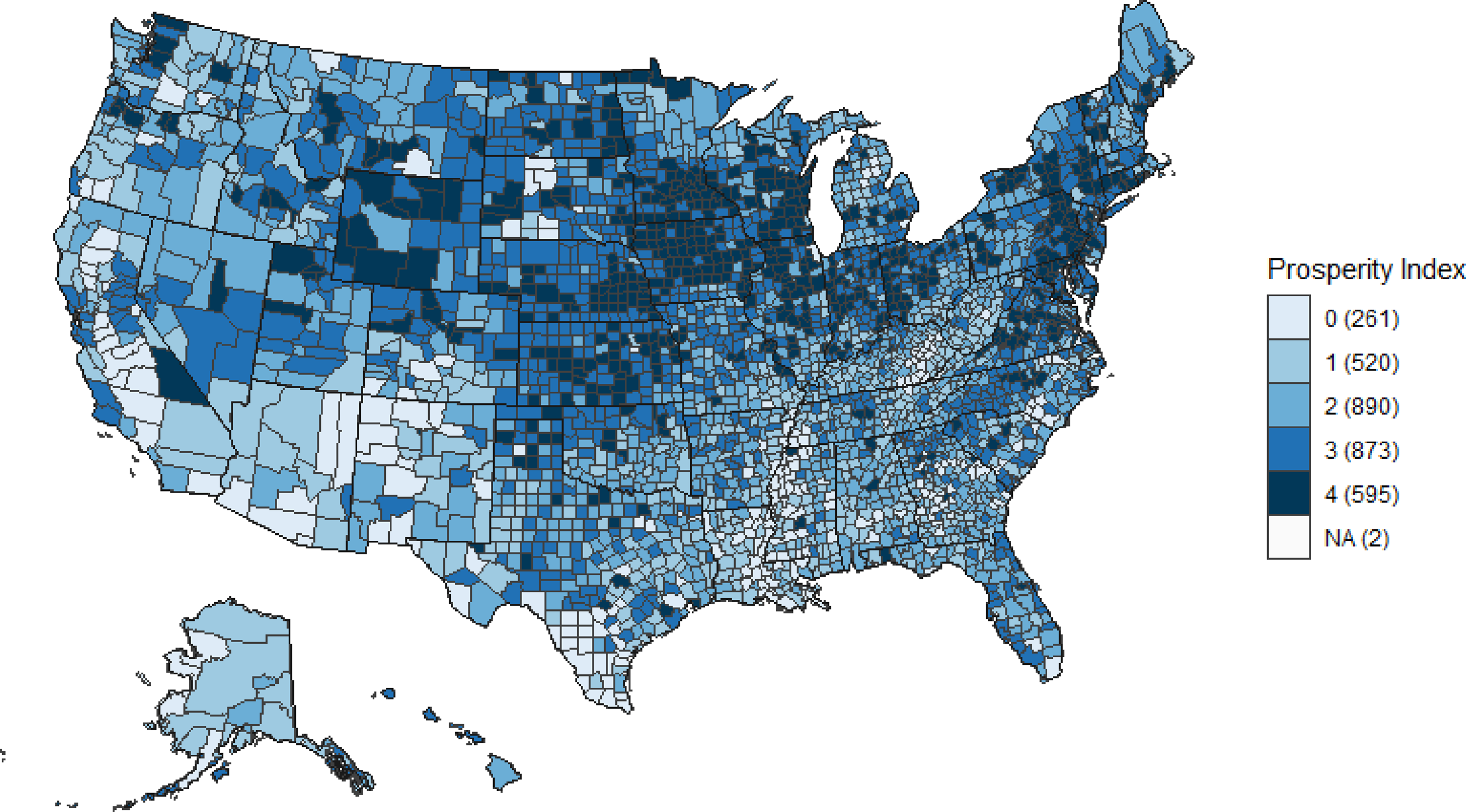

Figure A2.

County-level map of 2000 IFW index.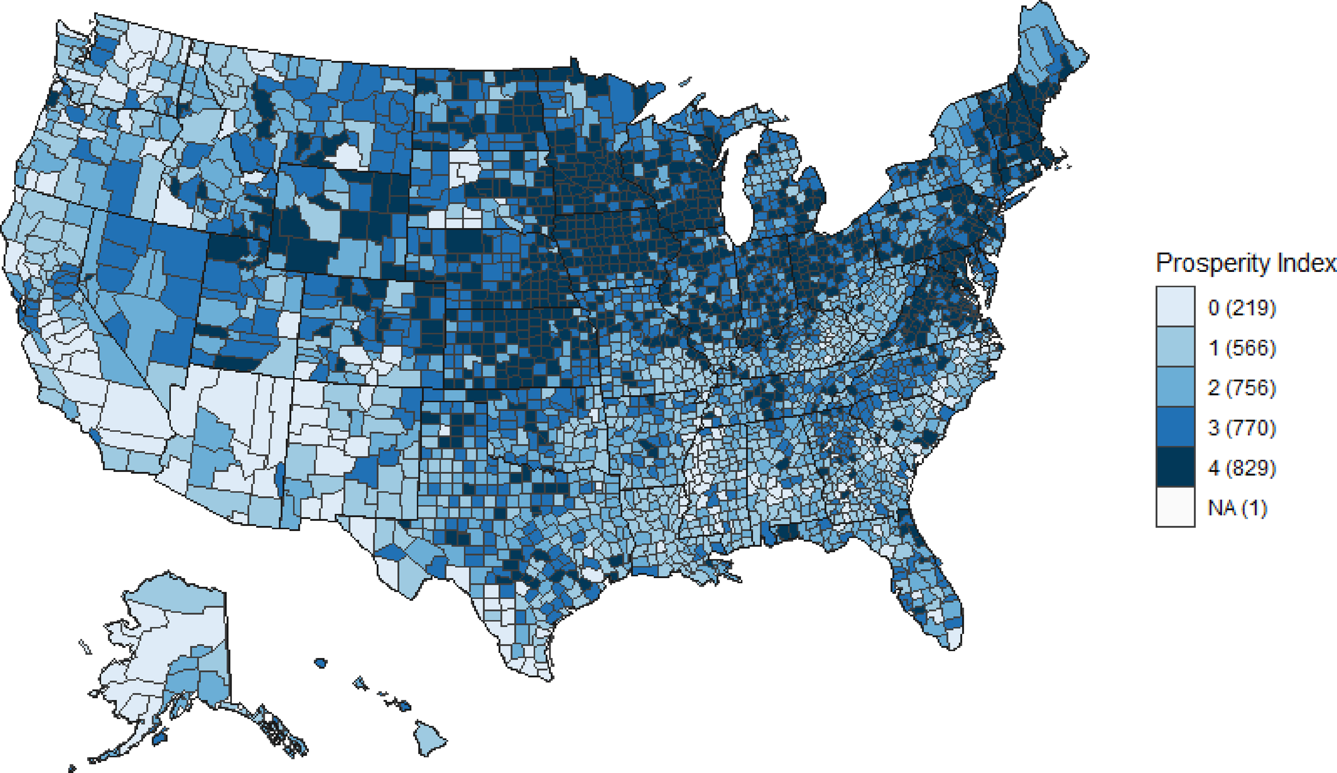

Figure A3.

County-level map of ∼2010 IFW index.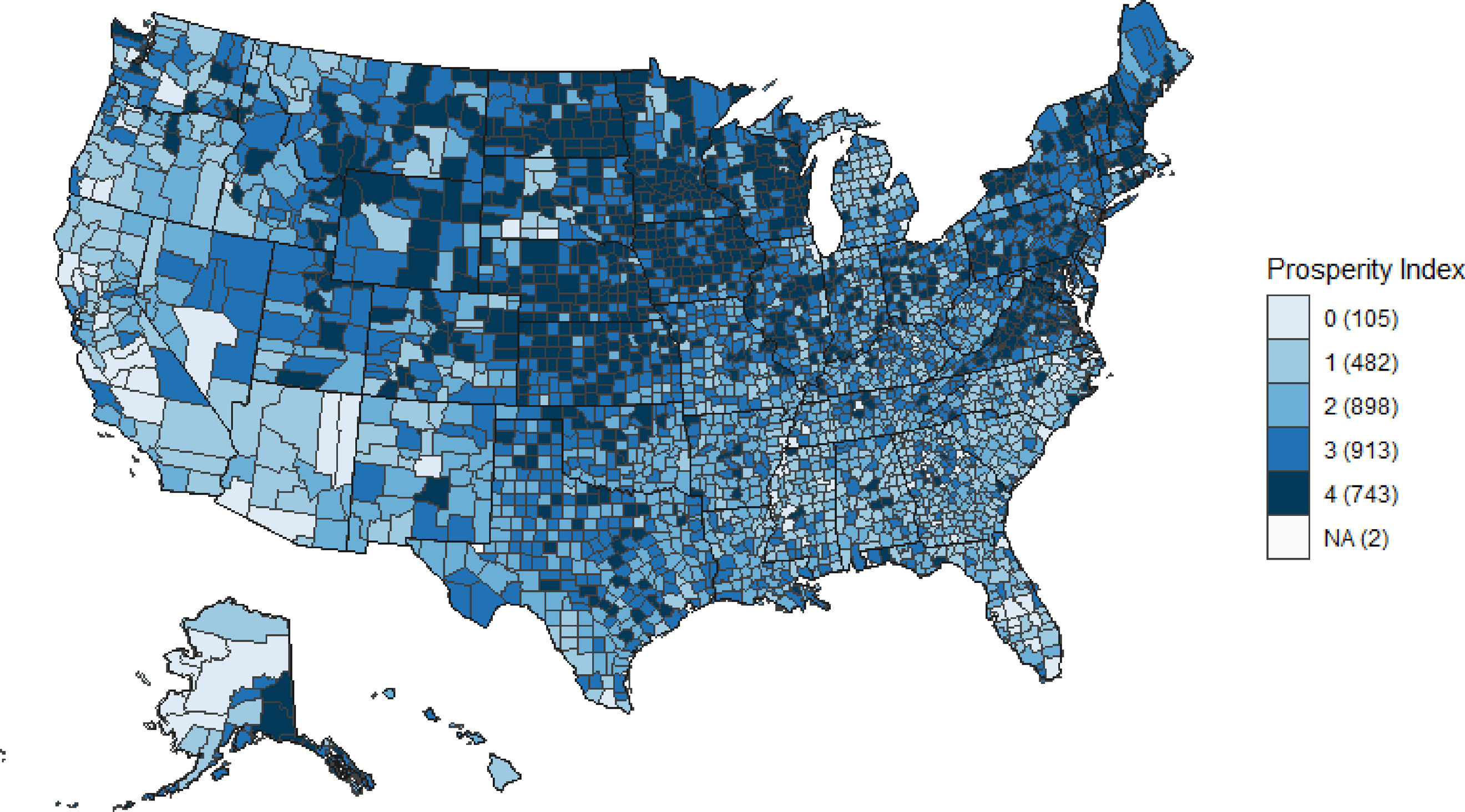

Figure A4.

County-level map of ∼2020 IFW index.

References

Abbott

Andrew

. 1995. “Sequence Analysis: New Methods for Old Ideas.” Annual Review of Sociology 21: 93–113. doi:10.1146/annurev.so.21.080195.000521.

Artz

Georgeanne M.

Hall

Arthur P.

Orazem

Peter

. 2005. Exaggerated Tales of Rural Economic Decline. No. 050225. Brandmeyer Center for Applied Economics, School of Business, University of Kansas.

Barkley

David L.

2008. “Evaluations of Regional Competitiveness: Making a Case for Case Studies.” The Review of Regional Studies 38 (2): 121–43. doi:10.52324/001c.8260.

Bell

Michael M.

2007. “The Two-Ness of Rural Life and the Ends of Rural Scholarship.” Journal of Rural Studies 23 (4): 402–15. doi:10.1016/j.jrurstud.2007.03.003.

Booi

Hester

Boterman

Willem R.

. 2020. “Changing Patterns in Residential Preferences for Urban or Suburban Living of City Dwellers.” Journal of Housing and the Built Environment 35 (1): 93–123.

Browning

Kellen

Johns

Louise

. 2024. “Big Sky, Big Growth: How Montana’s Newcomers Are Shaping its Senate Duel.” The New York Times; May 26, 2024, sec. U.S. https://www.nytimes.com/2024/05/26/us/politics/montana-senate-bozeman-growth.html

Coburn

Andrew F.

MacKinney

A. Clinton

McBride

Timothy D.

Mueller

Keith J.

Slifkin

Rebecca T.

Wakefield

Mary K.

. 2007. “Choosing Rural Definitions: Implications for Health Policy.” Rural Policy Research Institute Health Panel Issue Brief; #2, March.

Coffman

Chad D.

Sunny

Sanwar A.

. 2021. “Reconceptualizing Necessity and Opportunity Entrepreneurship: A Needs-Based View of Entrepreneurial Motivation.” Academy of Management Review 46 (4): 823–825. doi:10.5465/amr.2019.0361.

Connor

Dylan S.

Xie

Siqiao

Uhl

Johannes H.

, et al. 2024. “Spatial Poverty Dynamics and Social Mobility in Rural America.” Population, Space and Place 30: e2802. doi:10.1002/psp.2802.

10.

Curtis

Katherine J.

Lee

Junho

O’Connell

Heather A.

Zhu

Jun

. 2019. “The Spatial Distribution of Poverty and the Long Reach of the Industrial Makeup of Places: New Evidence on Spatial and Temporal Regimes.” Rural Sociology 84 (1): 28–65. doi:10.1111/ruso.12216.

11.

Deller

Steven C.

Conroy

Tessa

. 2022. “Regional Economic Trends Across the Urban-Rural Divide.” In Rural Areas in Transition, edited by Walzer

Normal

Merret

Christopher

, 19–44. Routledge.

12.

Deller

Steven

Parr

Jackson

. 2021. “Does Student Loan Debt Hinder Community Well-Being?” International Journal of Community Well-Being 4: 263–285. doi:10.1007/s42413-020-00107-1.

13.

Dissart

J.-C.

Deller

Steven C.

. 2000. “Quality of Life in the Planning Literature.” Journal of Planning Literature 15 (1): 135–161. doi:10.1177/08854120022092962.

14.

Dsouza

Nishita

Carroll-Scott

Amy

Bilal

Usama

Headen

Irene E.

Reis

Rodrigo

Martinez-Donate

Ana P.

. 2023. “Investigating the Measurement Properties of Livability: A Scoping Review.” Cities & Health 7 (5): 839–853. doi:10.1080/23748834.2023.2202894.

15.

Etuk

Lena E.

Acock

Alan

. 2017. “Toward a Rural Community Vitality Measurement Practice.” Community Development 48 (1): 141–53. doi:10.1080/15575330.2016.1251480.

16.

Francois

Jean R.

Katherine

S. Nelson

Burchfield

Emily K.

. 2024. “Linking Diversity–Productivity Conditions of Farming Systems with the Well-Being of Agricultural Communities.” Sustainability 16 (16): 6826. doi:10.3390/su16166826.

17.

Fuguitt

Glenn V.

Brown

David L.

. 1990. “Residential Preferences and Population Redistribution: 1972–1988.” Demography 27 (4): 589–600.

18.

Gabadinho

Alexis

Ritschard

Gilbert

Müller

Nicolas S.

Studer

Matthias

. 2011. “Analyzing and Visualizing State Sequences in R with TraMineR.” Journal of Statistical Software 40: 1–37. doi:10.18637/jss.v040.i04.

19.

Galpin

Charles Josiah

. 1915. “The Social Anatomy of an Agricultural Community.” University of Wisconsin Agricultural Experiment Station Research Bulletins 20 (38): 1–34.

20.

Green

Gary Paul

Zinda

John Aloysius

. 2014. “Rural Development Theory.” In Handbook of Rural Development, edited by Green

Gary Paul

, 3–20. Edward Elgar Publishing.

21.

Isserman

Andrew M.

2001. “Competitive Advantages of Rural America in the Next Century.” International Regional Science Review 24 (1): 38–58. doi:10.1177/016001701761013006.

22.

Isserman

Andrew M.

2005. “In the National Interest: Defining Rural and Urban Correctly in Research and Public Policy.” International Regional Science Review 28 (4): 465–99. doi:10.1177/0160017605279000.

23.

Isserman

Andrew M.

Feser

Edward

Warren

Drake E.

. 2009. “Why Some Rural Places Prosper and Others Do Not.” International Regional Science Review 32 (3): 300–342. doi:10.1177/0160017609336090.

24.

Jolliffe

Dean

. 2003. “Nonmetro Poverty: Assessing the Effect of the 1990s.” ERS Feature: Rural Poverty & Well-Being (blog); September 1. https://www.ers.usda.gov/amber-waves/2003/september/nonmetro-poverty-assessing-the-effect-of-the-1990s/

25.

Kashef

Mohamad

. 2016. “Urban Livability Across Disciplinary and Professional Boundaries.” Frontiers of Architectural Research 5 (2): 239–53. doi:10.1016/j.foar.2016.03.003.

26.

Khatiwada

Lila K.

2014. “Modeling and Explaining County-Level Prosperity in the U.S.” Journal of Regional Analysis and Policy 44 (2): 143–56. doi:10.22004/ag.econ.243970.

27.

Klaesson

Johan

Wixe

Sofia

. 2023. “Place and Immigrant Labour Market Integration: A Sequence Analysis Approach.” European Urban and Regional Studies 30 (4): 404–29. doi:10.1177/09697764231166358.

28.

Levine

Marc V.

2020. The State of Black Milwaukee in National Perspective: Racial Inequality in the Nation’s 50 Largest Metropolitan Areas, 56. Center for Economic Development Publications. University of Wisconsin. https://dc.uwm.edu/ced_pubs/56

29.

Lipsitz

George

. 2011. “Introduction: Race, Place and Power.” In How Racism Takes Place, 1–21. Temple University Press.

30.

Lohr

Kathy

. 2008. “Georgia’s Clayton County Schools Lose Accreditation.” NPR; August 29, 2008, sec. Education. https://www.npr.org/2008/08/29/94095347/georgias-clayton-county-schools-lose-accreditation

31.

Longman

Ryan J.

Diaz

Henry F.

Giambelluca

Thomas W.

. 2015. “Sustained Increases in Lower-Tropospheric Subsidence Over the Central Tropical North Pacific Drive a Decline in High-Elevation Rainfall in Hawaii.” Journal of Climate 28 (22): 8743–59. doi:10.1175/JCLI-D-15-0006.1.

32.

Losacker

Sebastian

Kuebart

Andreas

. 2024. “Introducing Sequence Analysis to Economic Geography.” Progress in Economic Geography 2 (1): 100012. doi:10.1016/j.peg.2024.100012.

33.

Manson

Steven

Schroeder

Jonathan

Van Riper

David

, et al. 2023. IPUMS National Historical Geographic Information System. Dataset. doi:10.18128/D050.V18.0.

34.

Messer

Benjamin L.

Dillman

Don A.

. 2011. “Comparing Urban and Rural Quality of Life in the State of Washington.” In Investigating Quality of Urban Life: Theory, Methods, and Empirical Research, 315–343. Springer Netherlands.

35.

Mulligan

Gordon F.

1984. “Agglomeration and Central Place Theory: A Review of the Literature.” International Regional Science Review 9 (1): 1–42. doi:10.1177/016001768400900101.

36.

Mulligan

Gordon F.

Partridge

Mark D.

Carruthers

John I.

. 2012. “Central Place Theory and its Reemergence in Regional Science.” The Annals of Regional Science 48: 405–431. doi:10.1007/s00168-011-0496-7.

37.

Okulicz-Kozaryn

Adam

. 2013. “City Life: Rankings (Livability) Versus Perceptions (Satisfaction).” Social Indicators Research 110 (2): 433–51. doi:10.1007/s11205-011-9939-x.

38.

O’Connell

H. A.

2012. “The Impact of Slavery on Racial Inequality in Poverty in the Contemporary U.S. South.” Social Forces 90 (3): 713–34. doi:10.1093/sf/sor021.

39.

Park

SooJin

Deller

Steven

. 2021. “Effect of Farm Structure on Rural Community Well-Being.” Journal of Rural Studies 87: 300–313. doi:10.1016/j.jrurstud.2021.09.014.

40.

Rahe

Mallory L.

2009. Rural Eutopia: Can We Learn from Persistently Prosperous Places? PhD Thesis. University of Illinois at Urbana-Champaign. https://www.ideals.illinois.edu/items/14314/bitstreams/50806/data.pdf

41.

Schmidt

Claudia

Deller

Steven C.

Goetz

Stephan J.

. 2024. “Women Farmers and Community Well‐Being Under Modeling Uncertainty.” Applied Economic Perspectives and Policy 46 (1): 275–299. doi:10.1002/aepp.13406.

42.

Shelly

Nora

. 2023. “Bozeman’s ‘Invisible Crisis’ of Homelessness is Increasing.” Bozeman Daily Chronicle; December 22, 2023. https://www.bozemandailychronicle.com/news/city/bozeman-s-invisible-crisis-of-homelessness-is-increasing/article_80486450-9f8e-11ee-a763-1bbe5b04a7b9.html

43.

Turkoglu

Handan

. 2015. “Sustainable Development and Quality of Urban Life.” Procedia-Social and Behavioral Sciences 202: 10–14. doi:10.1016/j.sbspro.2015.08.203.

44.

Veréb

Vanda

Marques

Carla

Madureira

Livia

Marques

Carlos

Keryan

Tigran

Silva

Rui

. 2024. “What is Rural Well‐Being and How is it Measured? An Attempt to Order Chaos.” Rural Sociology. doi:10.1111/ruso.12536.

45.

Waldorf

Brigitte

. 2007. What is Rural and what is Urban in Indiana. Purdue Center for Regional Development.

46.

Wei

Kailei

Wang

Weilin

Shah

Fahad

. 2023. “Spatial and Temporal Characteristics of Rural Livability and its Influencing Factors: Implications for the Development of Rural Revitalization Strategy.” Environmental Science and Pollution Research 30 (17): 49162–79. doi:10.1007/s11356-023-25748-5.

47.

Wilson

Bev

Rahe

Mallory L.

. 2016. “Rural Prosperity and Federal Expenditures, 2000–2010.” Regional Science Policy & Practice 8 (1–2): 3–26. doi:10.1111/rsp3.12070.

48.

Yurui

Luyin

Qiao

Qianyi

Wang

Karácsonyi

David

. 2020. “Towards the Evaluation of Rural Livability in China: Theoretical Framework and Empirical Case Study.” Habitat International 105: 102241. doi:10.1016/j.habitatint.2020.102241.

Prosperity Across the United States: Revisiting the Isserman,Feser,and Warren Prosperity Index Using Sequence Analysis

Abstract

Keywords

Introduction

Measuring Prosperity

The Isserman, Feser, and Warren Prosperity Index

Data & Methods

Findings

Evaluating Prosperity Pathways

Prosperity Across Geography

Prosperity Across the Urban-Rural Continuum

Prosperity Over Time: Stability and Change

Conclusion

Footnotes

Acknowledgements

ORCID iDs

Funding

Declaration of Conflicting Interests

Data Availability Statement

Notes

Appendix

References