Sage Journals: Discover world-class research

Abstract

For decades, gravitational analysis has been a key instrument in analyzing spatial flows. Time and again, it has prompted new and challenging research questions. This paper provides a concise overview of the foundation, the conceptualization and empirical relevance of gravitational principles in regional science and spatial economics. Attention is also given to general “social physics” interpretations of gravity in spatial interaction models and to the impact of intangible distance frictions. The main emphasis in the study is placed on the significance of spatial impedance functions and gravity potential analysis. In particular, the paper focuses on cross-border trade and has three main goals: (i) to address the robustness of distance friction parameters related to trade borders, employing, inter alia, quantitative results from meta-analyses on trade models in spatial economics; (ii) to present a promising methodology based on gravity potential and the related gravitational gradient models that include directional intensities of flows; (iii) to test the validity of the latter approach on the basis of a vector gradient analysis of export patterns of the Netherlands. The paper argues that—despite the space-reducing impact of the modern digital technologies—gravitational principles still have an uncontested relevance in an analysis of spatial flows in regional science.

Keywords

gravity theory spatial interaction models social physics entropy gravity potential distance friction elasticity vector gradient

Introduction

Any human effort to attract goods, services or contacts from outside the home area needs trade, transport or communication. This premise is of particular relevance when the inclusive costs of home production (comprising all generalized transport costs, including psychological ones) exceeds the costs of production taking place elsewhere. Thus, relative cost differences (in particular, the border-crossing costs) between regions or countries, in combination with spatial productivity differences, largely affect the volume, nature and composition of cross-border trade, transportation and communication flows. There is extant literature in the area of international economics, economic growth theory, regional economics, transportation science and the new economic geography focusing on the foundations and appearances of cross-border linkages. Special attention has been paid to industrial heterogeneity, taste variety, differences in factor productivity caused by various inputs, and territorial competitiveness advantages (see e.g. Williamson 1967; Baldwin and Wyplosz 2004; Bröcker 2020). Given the efficiency gains from spatial interaction, all actors involved in cross-border flows will normally face a win-win situation for the domestic market (though not necessarily equal for all individual industrial sectors, population segments, labor markets or places; see Reggiani et al. 2012).

Beside the competitive cost and efficiency returns, there are other advantages that co-determine cross-border linkages. Depending on the size of the production and the consumer market, there is also a wide variety of production scale advantages, especially in areas with large industrial concentrations specializing in specific goods and services. Similar scale (and agglomeration) arguments hold true for technological innovation advantages in geographical space, e.g. in innovation districts (Romer 1994). The scale advantage argument is in line with Adam Smith’s (1776) view that large-scale production prompts efficiency-enhancing labor specialization. In the past decades, similar perspectives were offered in the new economic geography and the new trade theory, especially from a monopolistic competition perspective (see e.g. Dixit and Stiglitz 1977; Krugman 1979; Capello and Nijkamp 2020).

Economic activities (including trade) do not take place in a “wonderland of no spatial dimensions” (Isard 1956) but typically are confronted with the challenge of overcoming multiple barriers: physical, political, social and cultural. At the same time, cross-border trade may be facilitated by infrastructure improvements, efficient border procedures or electronic customs services, which may favor openness and globalization, and the resulting competitiveness (Crafts and Venables 2001; Yi 2003). On the contrary, strict trade barriers lead to high spatial interaction costs which would not exist in a perfect open world (Nijkamp 2021).

In the early days of the emergence of trade theory, most attention was paid to tangible barriers (e.g. mountains, rivers, customs barriers) which led to friction costs which are relatively easy to measure. More recently, we observe also a profound interest in intangible barriers such as institutional inertia, cultural impediments, political resistance, etc. (an informed overview in Linders 2006). Clearly, international or interregional trade takes place in a complex force field of intertwined spatial economies. The exchange of goods and services between countries and regions exerts a welfare-enhancing effect on consumers or agents in the respective countries or regions (see Andersson and Andersson 2017). Clearly, depending on the relative trade advantages and competences of the various players involved, the intensity and the composition of trade may vary from one area to another.

International economics and trade theory have developed various analysis frameworks to understand the origin and structure of trade and to provide policy lessons for an open and global economy. A point in case is Adam Smith’s theory of absolute advantage, David Ricardo’s theory of comparative advantage, the classical Dornbusch-Fisher-Samuelson trade approach, the standard Heckscher-Ohlin trade model (and its many extensions), the Leontief Input-Output model etc. (a review in Zielińska-Głębocka 2012; Starck 2012). Despite the great variety of conceptual and theoretical foundations of trade analysis in economics, notably most operational studies of international or interregional trade are, directly or indirectly, based on a common analysis framework, viz. the well-known gravity model.

The gravity model is undoubtedly the most popular and operational trade and spatial interaction model and has a long history (Anderson 1956; see also Section “A Brief History of Gravity Analysis in Regional Science”). The first thorough gravity application in macro-economics was presented by Tinbergen (1962), while later on, Linnemann (1966) developed a fully operational gravity model for international trade. However, in the context of trade, the conceptual foundation of the gravity model in geography was laid much earlier, by Janowski in 1908. Unfortunately, his study remained unknown due to the fact that it was published in Polish. A recent translation into English is provided in Janowski ([1908] 2013).

This paper has three specific aims. First, it offers a concise discussion of the history, the complementary side-roads and the vast application potential of the gravity model in regional science and geography, and in spatial sciences in general (including trade theory). Another aim is to highlight the importance of spatial impedance frictions such as spatial elasticities to trade and flows, both conceptually and empirically. Last but not least, a new perspective on gravity principles is offered by modeling and interpreting international trade flows by means of gravity potential models and gravitational gradient models, using Dutch export flows as a test case.

The paper is organized in the following way: the introductory section is followed by “A Brief History of Gravity Analysis in Regional Science” section with a concise sketch of the rich history, contours and application fields of gravitational analysis in regional science, geography, and trade/transport analysis. “Gravitational Analysis in Spatial Economics” Section highlights the basic gravity model and its variants, while “The Robustness of Distance -Friction Elasticities in Gravity Models: A Meta-Perspective” Section presents some findings from meta-analyses of gravity characteristics in heterogeneous trade flows, with special emphasis placed on friction elasticities. Next, in “Gravity Potential Modeling: Scalar and Vector Analysis of Spatial Flows” Section, we present gravitational analysis in a novel context of geographical accessibility in trade through gravity potential modeling and vector gradient analysis in international trade. “Gravity Potential Modeling of Dutch Trade Flows: An Example” Section is devoted to an illustrative application of directional gravity potentials for Dutch trade flows. The paper concludes with retrospective and prospective explorations of pathways for gravitational analysis in regional science.

A Brief History of Gravity Analysis in Regional Science

Early Contributions

The Newtonian gravitational model—initially developed and applied in physics—boasts a long history of several centuries in many sciences. It describes the impact of distance on the interaction between material objects in space. Over the last hundred years, the model has been largely applied in other disciplines such as astronomy, sociology, anthropology, biology, social psychology, demography, trade theory, and spatial sciences (including regional science, economic geography, trade theory, and transportation economics). Especially in spatial sciences, the gravity model has prompted a plethora of advanced quantitative research, notably in the context of spatial interaction models (including entropy models).

The gravity model was originally introduced to physics by Isaac Newton ([1686] 1999) in his seminal work on modern science, “Philosophiae Naturalis Principia Mathematica” (Mathematical Principles of Natural Philosophy) in the following standard form:

F = G \frac{M_{1} M_{2}}{r^{2}},

where:

F = gravity power,

M₁, M₂ = masses of two interacting bodies,

r = Euclidean space between the bodies’ centers,

G = gravitational constant.

In its standard formulation, the Newtonian gravity model has three important general characteristics:

It describes the interaction between two bodies; in a system consisting of more than two bodies (e.g., three), its dynamic trajectory may lead to chaos as proven by Poincaré in 1890 (see Stewart 2002).

The bodies’ masses and the physical distance between them are unambiguously defined.

The exponent of the power function in the denominator amounts to exactly 2, and is invariant.

Notably, in gravity models used later in other scientific disciplines, the last two properties are not necessarily maintained. On the other hand, these properties have been subjected to a wealth of applied research, e.g. in spatial economics and spatial econometrics. This holds true not only for the gravity model used in the analysis of international trade, but also (more generally) in spatial sciences in relation to transport, commuting or migration.

Most probably, the use of gravity theory as an analytical concept for human and spatial interactions in social sciences was first advocated by Carey (1858) who interpreted the interaction between points or groups in space in a way analogous to gravitation. His principal statement was: “Men tends, of necessity, to gravitate towards his fellow man” (p. 42). His pioneering work was operationalized for the first time in a study on migration flows between cities in the UK by Ravenstein (1885) who described spatial interaction between areas or groups in a standard gravity format. With the exception of Janowski ([1908] 2013), it took several decades before the gravity concept was furthered as an operational and testable proposition into spatial sciences. The noteworthy pioneers in the first part of the twentieth century included—with different scientific foundations and applications—Young (1924), Reilly (1931), Stewart (1941), Converse (1949) and Zipf (1949).

A New Wave of Interest

After WWII, it was in particular Isard (1956) who drew attention to the large operational scope and predictive potential of gravity models in regional science. From the mid-1950s onward, the gravity model gained increasing popularity in regional science (in particular, in interregional transport studies and retail models). Almost at the same time, gravity models entered international economics (in particular, in international trade theory; see Tinbergen 1962). Meanwhile, in both domains of spatial-economic research, i.e. regional science and international economics, the gravity model enjoyed an established position. A huge number of publications on the theory and application of gravity models in regional science emerged in the second part of the twentieth century (see e.g. Gould 1972; Batty 1976; Isard and McLaren 1982; Haynes and Fotheringham 1984; Foot 1987; Fotheringham and O’Kelly 1989; Nijkamp and Reggiani 1992; Sen and Smith 1995). The use of gravity models in a broad range of the spatial interaction phenomena is at present a dominant research practice in spatial sciences. Consequently, there is hardly any spatial interaction model not directly or indirectly inspired by the Newtonian law of gravitation.

Gravitational forces in spatial systems are—as mentioned above—based on relational interactions which are governed by spatial interdependences in the form of spatial attraction forces between two or more points in geographic space. Gravitation theory says that these attraction forces are proportional to the respective masses of the points and inversely proportional to their squared distances. Several authors have pioneered the development and conceptualization of gravity theory for spatial systems. The early contributors to regional science include in particular Isard (1960), Lukermann and Porter (1960), Batty (1970), Chisholm and O’Sullivan (1973), Isard and MacLaren (1982), followed by many others. This has ultimately led to the emergence of a well-known class of models, referred to as spatial interaction models.

Let us pause for a terminological remark: in a strict sense, the popular use of the term “gravity model” is not entirely correct. In most applications in spatial economics and geography, various types of spatial interaction models are used that may have a formal analogy to Newton’s gravity approach (Stewart 1941), but often have a much wider scope, as they deal in a consistent way with marginal constraints (Wilson 1970; Bröcker 2020). There are numerous studies however, where the concepts of gravity model and spatial interaction model are used interchangeably (see e.g. Niedercorn and Bechdolt 1969; Haynes and Fotheringham 1984; Sen and Smith 1995; Wilson 2000). Especially in the economics of international trade, the term “gravity model” is quite common, following the pioneering study of Tinbergen (1962); see, for instance, Krugman (1979).

Social Physics

There has been a parallel strand of literature on spatial sciences which also go back to gravitational principles, called social physics or, more recently, econophysics (see e.g. Mantegna and Stanley 2000). This approach started from the general class of spatial interaction models in social sciences and has gained much popularity in geography and regional science, starting with the seminal work of Wilson et al. (1969).

The social physics approach seeks, in general, use of principles from physics as a foundation for an analytical study of interactions in social science phenomena (e.g. migration, tourism, commuting). Next to standard gravitation theory and variants thereof, complementary approaches have gained much attention, in particular entropy theory (see e.g. Wilson 1970; and Wilson and Bennett 1985). The main idea is that the “mechanistic” nature of physics models may take a behavioral and relevant twist in social science interpretations of spatial interaction phenomena, based on probabilistic states of a spatial interaction system.

Beside the principles of physics, the entropy approach finds its origin in information theory (a general exposition in Theil 1967). The entropy principle in spatial interaction models aims to identify the most probable state of a system of flows. Snickars and Weibull (1977) offer a thorough information-theoretic foundation and interpretation of entropy models in social physics while Nijkamp (1975) provided a cost-minimization interpretation.

Nijkamp and Reggiani (1992) offered a broad exposition on the justification of social physics, including its methodological underpinning, based on spatial interaction theory, cost-efficiency principles, aggregate utility theory, statistical information theory, and micro-based choice theory (see also an informative overview by Bröcker 2020). A special class of approaches in the area of spatial interaction models can be found in the so-called intervening opportunities principles (see Stouffer 1969) and in the class of potential (or spatial attraction) models often used in retail studies. Over the past decades, spatial interaction models—either originating from standard gravity theory or from spatial entropy theory—have gained great popularity in analyses of flows in regional science, geography, demography and sociology. As argued by Couclelis (2009), entropy-based spatial interaction theory indicates a significant enrichment of the conventional Newtonian-based gravitational theory: “Wilson’s seminal statistical-mechanical derivation of spatial interaction (formerly “gravity”) models rescue these from the prevailing and the planetary analogizing, while also providing a philosophically significant insight into the value of an informational—as opposed to empiricist—perspective” (p. 80).

From an operational perspective, the measurement of masses and of distance frictions in a gravity-based trade model is not always easy (see also the previous sections). In addition to tangible barriers to spatial interaction, there are intangible distance frictions such as information barriers, cultural impediments, trade policy conflicts, language barriers, malfeasance in trade, etc. (see e.g. Poot 2004). Culture (including trust) and institutional solidity are decisive factors of the occurrence of cross-border or spatial interaction phenomena. This is also of importance to an analysis of spatial coherence and compact patterns. An illustrative early example of a study on the impact of (immaterial) culture on cross-border communication or interaction is provided in an early article by Klaassen, Wagenaar, and Van der Weg (1972) on the impact of language differences on the intensity of telecommunication flows between Flemings and Walloons in Belgium. Over the past two decades, there has been an abundance of non-material spatial interaction analyses. Examples of studies on cultural-institutional barriers include Anderson and Van Wincoop (2003), Beugelsdijk, de Groot, and van Schaik (2004), Combes, Lafourcade, and Mayer (2005), Guiso, Sapienzo, and Zingales (2004), Hutchinson (2002), Rauch (2001), Rauch and Trindade (2002), and Tranos and Nijkamp (2013). Finally, Linders (2006) also offers a plethora of empirical studies on intangible barriers (e.g., culture or institutions) in spatial interaction models.

It is an important statistical question whether a negative power-law function or a negative exponential function for the distance friction in a gravity model or spatial interaction model needs to be used (see e.g. Fotheringham and O’Kelley 1989; Wilson 2000). The power-law specification is a direct implication of a Newtonian gravitational approach that is commonly used in international trade modeling. It implies constant distance elasticities. However, there are numerous applications outside trade analysis, especially in the context of spatial interaction analysis, that employ exponential distance decay functions or alternative specifications (further discussion in Östh, Lyhagen, and Reggiani 2016).

It is also noteworthy that recently, a new trend has emerged in spatial interaction analysis and spatial flows models, based on modern proximity theory. Proximity is the counterpart of distance friction and aims to address the general attraction factors between two or more phenomena (a solid analysis in Torre and Wallet 2014, and a quantitative approach in Caragliu 2015). Proximity is not only a geographical phenomenon but is also expressed in terms of intensity of social relations, cultural similarity, technological cooperation, and the like. Gravitational principles of spatial interaction appear to apply also to quantitative spatial proximity studies. Applications and further studies can be found in Caragliu (2015), Caragliu and Nijkamp (2012), Kourtit (2016), and Tranos and Nijkamp (2013), to name a few. It is foreseeable that proximity analysis—as part of a behavioral force field research—will gradually be recognized in spatial interaction analysis.

Finally, it should be noted that over the past decades, various new directions in geographical applications of the gravity model have come to the fore, in particular on the man-made and political nature of distance barriers, the impacts of non-material flows, the dynamics of borders and the impact of digital (“spaceless”) technology. These issues in regional science and spatial economics are covered by Bröcker (1984), Deardorf (1998), Eichengreen and Irwin (1998), Frankel (1997), Linders (2006), Tranos and Nijkamp (2013), Bröcker (2020) and Nijkamp (2021) and others. In this study, we present alternative or complementary foundations of the gravity model for international trade analysis, drawing on geographic potential analysis. Before doing so, in the next section (“Gravitational Analysis in Spatial Economics” Section) we highlight the empirical importance of gravitational analysis for inter-country trade transport. This is followed by a presentation and discussion of the robustness of gravitational distance-friction coefficients—interpreted as elasticities—in cross-border trade models (“The Robustness of Distance-Friction Elasticities in Gravity Models: A Meta-Perspective” Section).

Gravitational Analysis in Spatial Economics

As mentioned, the Newtonian gravity principle has been largely applied in spatial economics (trade theory, transport economics, commuting patterns, migration theory etc.). In this section, we address in particular international cross-border flows and international trade. Trade flows mirror the mutual economic connectivity between countries. Therefore, it is conceivable that the gravity model—with numerous varieties—has often been used to analyze and map out the factors determining cross-border trade (see e.g. Mazurek 2016; Bröcker 2020). Another important reason is that the value of trade flows between pairs of countries is usually measurable, and hence provides a reliable basis for the econometric estimation of model parameters.

The widespread application of the gravity model in explaining and predicting flows in international trade has begun with the breakthrough work by Tinbergen (1962). We offer here a very concise description. His classical model had the form:

E_{i j} = α_{0} Y_{i}^{α_{1}} Y_{j}^{α_{2}} D_{i j}^{α_{3}},

while his extended model—with a view to the Netherlands’ trade position—was formulated as:

E_{i j} = α_{0} Y_{i}^{α_{1}} Y_{j}^{α_{2}} D_{i j}^{α_{3}} N^{α_{4}} P_{C}^{α_{5}} P_{B}^{α_{6}},

where:

E_ij—exports of country i to country j,

Y_i—GDP of origin country i,

Y_j—GDP of destination country j,

D_ij—distance between country i and country j,

N—dummy variable for neighboring countries,

P_C—dummy variable for Commonwealth preference,

P_B—dummy variable for Benelux preference,

α₀, α₁, α₂, α₃—parameters of the model.

These models were operationalized on the basis of export data from eighteen more developed countries in the world. The degree of adjusting these models to real data was for model (1): r² = 0.6724 (r = 0.82) and for model (2): r² = 0.7056 (r = 0.84), respectively. The introduction of three new variables in equation (3) increased the value of the r² only by 0.033, almost a negligible value. This was also noticed by Tinbergen: “Surprisingly enough, the introduction of three additional variables increased the correlation coefficient to 0.84 only” (Tinbergen, 1962, 266). Clearly, international trade is a mystery that calls for more evidence-based research on the puzzling issue.

Meanwhile, gravitational principles in spatial interaction models have gained much popularity. They have also been adjusted to different conceptual frameworks, such as Ricardian and Hecksher-Ohlin perspectives. As mentioned before, borders may be very heterogeneous in nature (Nijkamp 2021), so that the definition and specification of border impedance frictions in a gravity model of spatial interaction call for due attention. In particular, in (interregional or international) trade models the multilateral resistance between trading countries reflects both the importing and exporting country’s average trade impedance. Using a power function in a gravitational model for trade (like in the Tinbergen case) means a constant impedance (distance) elasticity. However, this way the relative power exerted by countries or regions in an open trade system could be disregarded. For instance, in their study on trade between the EU and the US, Krugman and Obstfeld (2009) found by correlating the relative size of EU countries (in % GDP) with the US share in trade exchange with EU countries, two groups of countries could be identified: (i) countries whose percentage share in trade with the US is bigger than the percentage size of their GDP (e.g. Ireland, the UK, the Netherlands); (ii) a remaining group with the opposite characteristics (e.g. France, Italy and Spain). The size of the economy and the border impedance clearly matters (see also Bergstrand 1985; McCallum 1995).

On the basis of this empirical study, a hypothesis may be advanced that trade exchange between two nations tends to grow if one partner’s economy is relatively bigger (cf. Krugman and Obstfeld 2009). If the economies of both partners are relatively small, trade exchange will also take place, but the volume will be smaller. This proposition is confirmed by simple empirical illustrative mapping of the size of Poland’s trade with the EU countries and the size of their GDP in 2015 (Figure 1).

Figure 1.

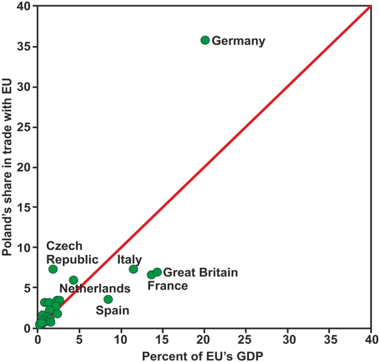
The size of European economies and the value of their trade exchange with Poland in 2015. Source: Own work based on EUROSTAT and Statistics Poland (2016).

Among the EU countries, Poland appears to enjoy the most intensive trade exchange with the biggest economies, i.e. Germany, Italy, the UK, and France. These are also countries with the biggest share of the GDP generated in the EU. The Czech Republic is an exception: Poland’s exchange is three times bigger than the Czech Republic’s GDP. The size of this country’s economy is different from that of the economies mentioned above, as it is significantly smaller. The situation is similar in countries like Lithuania, Slovakia and Hungary. They are Poland’s neighbors or are located in close vicinity. Poland’s trade exchange with all of them is approximately three times more intense than the GDP generated by these countries as compared to the overall EU GDP. This suggests clearly that the intensity of trade exchange between countries is also affected by the distance between the trading countries.

In relation to the former conclusions, the above proposition on distance frictions is a robust argument in favor of the use of the gravity model in explaining and predicting the spatial structure of international (or interregional) trade. Its simplest form is as follows:

T_{i j} = k \frac{{GDP}_{i} \cdot {GDP}_{j}}{d_{i j}^{β}},

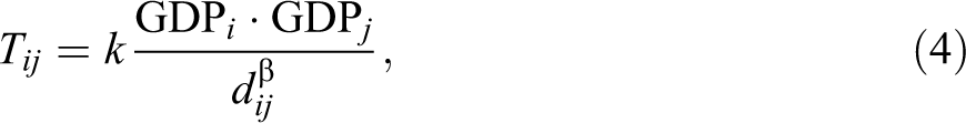
where:

T_ij = the value of trade between country i and country j,

k = the proportionality constant,

GDP_i = the GDP value of country i,

GDP_j = the GDP value of country j,

d_ij = distance between country i and country j,

β = exponent of a power function.

Despite a similar formal structure as in Newton’s model (1), our adjusted model (4) has the following features differentiating it from the traditional physical model:

Physical mass has been replaced by an economic value (GDP);

The distance is not strictly defined; this may be the geometric distance (Euclidean space), economic distance expressed by means of the interaction cost, or physical-geographical distance expressed in appropriate physical measurement units;

The exponent of the power function β and the constant K are not universally identical. Their values may change in time and space.

Therefore, despite the identical structure, model (4) employed in modeling cross-border trade flows is only an analogy to Newton’s model. As it has been mentioned, in order to enhance the precision of the assessment of trade relations between countries, gravity model has been subjected to numerous, oftentimes successful, modifications and amendments (see Salvatici 2013; Shepherd 2013). As argued above, a major empirical question is the value of the Newtonian distance friction coefficient. This issue is addressed in “The Robustness of Distance-Friction Elasticities in Gravity Models: A Meta-Perspective” Section.

The Robustness of Distance-Friction Elasticities in Gravity Models: A Meta-Perspective

The impedance function in a gravity model has been a source of much debate. By analogy to Newton’s gravitational principle, the expression of distance decay in spatial interaction assumes an inverse power function. In more recent history, an exponential distance friction function was also used (see Gould 1972; Haynes 1975; Hagget, Cliff, and Frey 1977), following the entropy-based spatial interaction model (Wilson 1970). For a profound conceptual and substantiative critique on these approaches please refer to Chen (2008, 2009, 2015). In recent years, we have witnessed a revival of power functions rather than exponential functions, mainly in the context of fractal dimensions of gravity (Batty and Longley 1994; Chen 2012).

In this section we address in particular the relevance of distance frictions, interpreted as elasticities in gravity analyses in spatial economics, in the context of a spatial impedance function. Elasticities are a standard concept introduced more than a century ago by Marshall (1842–1924) to gauge the relative impact of a price change on demand (see Krynski 1976). In the case of a power demand function, this price elasticity is constant, but in most cases elasticity is also a function of the prevailing price, the demand level and the size of the country.

Notably, the classical gravity model has a power function structure, so that a one percentage change in the (geometric or generalized) distance friction has also a percentage impact on the volume of bilateral trade equal to −β. This constant elasticity is an important feature of any gravity model. As mentioned already, especially in geography and regional science we observe also a frequent use of exponential distance friction functions (see Östh, Lyhagen, and Reggiani 2016). In the latter case, the distance elasticities may also be dependent on distance (or average travel costs). Further expositions on elasticity analysis can be found in Anderson (2010a); Anderson (2010b); Anderson and Yotov (2012); Bergstrand and Egger (2010); Brun et al. (2005); Carrére, De Melo, and Wilson (2009); Chaney (2013); De Benedictis and Taglioni (2011); Disdier and Head (2008); Head and Mayer (2010); Rautala (2015), and many others. There is also extant empirical literature on the empirics of the gravity model, starting from Tinbergen’s (1962) seminal contributions (see also Chaney 2013; Squartini and Garlaschelli 2014; or Almog, Bird, and Garlaschelli 2015). We first present interesting empirical findings on elasticity values, resulting from some meta analyses provided by literature on gravity modeling.

In 2008, Disdier and Head presented an in-depth meta-analysis of 103 studies and 1,467 estimated values of friction elasticity in gravity analysis (using a negative power function). Figure 2, drawn from their work (Disdier and Head 2008), indicates that the impact of distance did not change significantly until the 1970s, when it started to grow, as shown by the rise of |β|.

Figure 2.

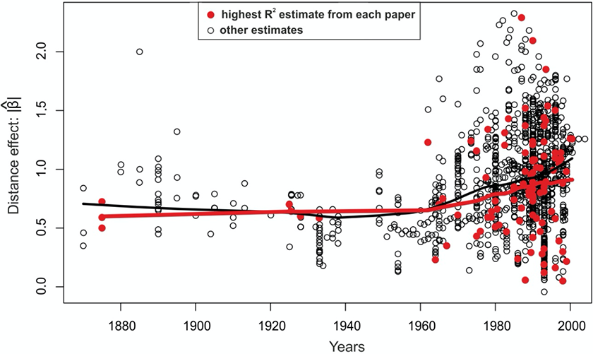
Changes in the impact of distance in gravity models in 1880–2000, showing an increase in elasticity |β|. Source: Disdier and Head (2008).

Next, Figure 3 presents the distribution of absolute β densities as well as their arithmetic mean (0.95) and their weighted arithmetic mean (using the inverse variance). Both approximate the modal value of distribution.

Figure 3.

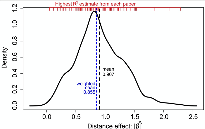
The estimated density of 1,467 |β| estimators. Source: Disdier and Head (2008).

Another meta-analysis, carried out later by Head and Mayer (2014: 160, Table 3.4)) on the basis of 159 studies by various authors and 2,509 estimations resulting from various methods, indicated that when all models are treated as one collection, the average elasticity amounted to (−0.93) (σ = 0.40). On the other hand, when only one category, namely structural gravity models, is taken into account,¹ the average elasticity appeared to be (−1.1) (σ = 0.41).

The most recent meta-analysis comprising 130 works and 1,470 estimated β’s was carried out by Tlustá (2015). Her results are close to the values presented by Disdier and Head (2008). The estimated average absolute elasticity β appeared to be 0.92. It is worth noting that its value does not decrease but tends to grow over time.

The three meta-analyses discussed above suggest that the average elasticity value approaches one. Therefore, in empirical gravity models the dependence between the intensity of trade flows and the distance friction tends to show an inverse proportionality. What is more, the absolute values of elasticity (β) tend to grow over time, i.e. the negative impact of the distance on the intensity of the trade exchange increases.

The latter conclusion defies the currently popular thesis of the diminishing (or even non-existent) role of distance in spatial relations due to the progress and wide-spread adoption of mainly information and communication technology (ICT). This is metaphorically referred to as “the death of distance” (cf. Cairncross 1997; Friedman 2005; Tranos and Nijkamp 2013). This issue was further examined by Carrére, De Melo, and Wilson (2009) who established the influence of distance on trade regionalization in countries with low incomes in 1970 and 2005. They employed four different methods to estimate the parameters of their gravity models. The average value of elasticity in 1970 amounted to –1.02, while in 2005 it was much higher, namely –1.2. Therefore, despite the expectations stemming from an increasing globalization, in the past 35 years the distinct role of distance between poorly developed countries has grown. This effect is sometimes referred to as a “distance puzzle.” For various reasons this may lead to a spatial segmentation of marginalized countries. The same conclusion was drawn by Brun et al. (2005). They examined, among others, the impact of distance on the volume of trade in 1962–1996, using a set of 130 countries, divided into three equivalent groups in the following combinations: Poor-Poor (P-P), Rich-Rich (R-R) and Poor-Rich (P-R). The estimated values of elasticity were as follows: P-P: –1.019, R-R: –0.716, and P-R: –0.978. Hence, distance appeared to weaken mostly the trade between poor countries (P-P). The research confirmed that “…poor countries have been marginalized by the recent wave of globalization while rich counties take advantage of the waning influence of the distance” (Brun et al. 2005, 115). Finally, Fratianni and Kang (2006) carried out even more in-depth research into the elasticity in gravity models. They took into consideration pairs of countries in seven configurations, as presented in Table 1.

Table 1.

Estimated Values of Elasticity.

	Configuration	Elasticity
1.	Both countries were OECD members	–0.73
2.	One country was an OECD member	–1.11
3.	Neither country was an OECD member	–1.29
4.	In both countries Christianity prevailed	–1.23
5.	In both countries Islam prevailed	–1.05
6.	In one country Christianity prevailed, in the other country Islam prevailed	–1.47
7.	Neither country was dominated by religion	–1.02

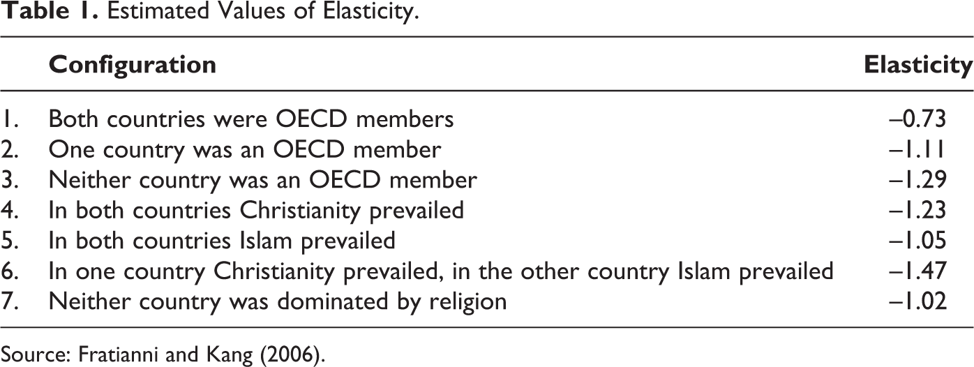
Source: Fratianni and Kang (2006).

Apparently, the values of elasticity as presented in Table 1 not only refer to distance frictions, but also to other relevant variables. They appear to vary depending on the culture, the level of development and religious-ethical traditions in the countries involved with international trade. Clearly, these countries are not homogeneous. These results also confirm the diversity in the spatial structure of international trade. This is because distance tends to have the smallest adverse effect on trade between the OECD countries or on those without a dominant religion. It is also worth noting that the elasticity is close to 1 in the case of countries where Islam is a dominant religion. We may thus conclude that the friction elasticity is an important factor correcting the gravitational effects in international trade, hence its spatial structure. Having now highlighted—conceptually and empirically—the role of distance frictions in gravitational analysis, in the next section we will focus on broader framing of gravitational principles in spatial sciences (including trade theory). We will resort to gravity potential analysis and present a new model that captures not only distance frictions, but also geometric spatial directions in a real world.

Gravity Potential Modeling: Scalar and Vector Analysis of Spatial Flows

Notably, gravitational principles in social physics allow for a profound analysis of spatial trade flows by using a scalar model of the gravity potential and, furthermore, also a geographic vector gradient field. These approaches fall under the general heading of gravity potential models.

Gravity Potential Model

The gravity potential model used in (spatial) economics does not directly refer to physical masses (such as the size of the population), but to the economic potential, related to the physical characteristics of a place of origin and destination. Examples of these proxies include income, capital or consumer expenditures. The inclusion of economic variables in the gravitation equation has brought gravity modeling into mainstream economics (see Starck 2012). As it has been mentioned, this approach was first applied by Tinbergen (1962) in his “Shaping the Word Economy”. His basic models have already been presented in equations (2) and (3).

Notably, in a standard gravity model the distance friction function does not affect the geographical direction of gravitational forces. This is less relevant in Newtonian gravitational analysis, but may be very important to the analysis of heterogeneous attraction forces in real-world geography.

From a modeling perspective, two prominent questions are to be raised in gravity-inspired international trade research: (i) given the variability in distance friction elasticities, how does trade accessibility of each individual country impact the relative volumes of imports and exports? (ii) given the fact that the impedance friction costs in a gravity model are determined only by distance, how are international trade patterns influenced by the location (i.e., the specific geographic coordinates) of each individual trading nation? This issue takes us into the realm of gravity potential theory (see also Chojnicki, Czyz, and Ratajczak 2011).

As presented by Gornisiewicz, Nijkamp, and Ratajczak (2020), the economic trade potential of a given country with respect to all other trading nations can be described by the following general gravity potential function (using GDP again as an expression of the strength of the potential field of accessibility):

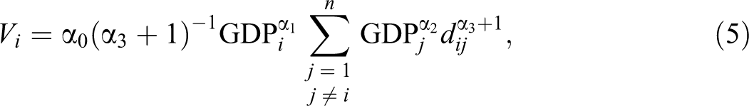
V_{i} = α_{0} {(α_{3} + 1)}^{- 1} {GDP}_{i}^{α_{1}} \sum_{\begin{matrix} j = 1 \\ j \neq i \end{matrix}}^{n} {GDP}_{j}^{α_{2}} d_{i j}^{α_{3} + 1},

In various empirical applications, the parameter $α_{3}$ may assume different values, which may lead to adjusted gravity potential functions (see for details Gornisiewicz, Nijkamp, and Ratajczak (2020)).

In regional science and geography research, usually a simplified expression of the geographic potential of a place is used, i.e.:

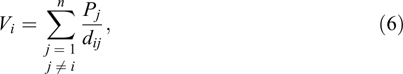
V_{i} = \sum_{\begin{matrix} j = 1 \\ j \neq i \end{matrix}}^{n} \frac{P_{j}}{d_{i j}},

where P_j stands normally for population mass (McCalden 1975). This expression has often been used in retail shopping models, urban facility use models and market area models. We note that equation (6) describing spatial accessibility is only valid if: (i) the distance friction coefficient $α_{3} = - 2$ ; and (ii) there is only a unit mass located in each point i (so that size does not matter for spatial effects) (an extensive argumentation in Sheppard 1979). These two conditions show the limited validity of the simplified geographical potential function, since: (i) as we have shown above, the numerical values of $α_{3}$ are mostly not equal to –2; (ii) a spatial anomaly (“potential inversion”) may arise: when a big and a small city are neighbors, the simplified potential model will predict that the small city has a disproportionally big mass. These two arguments require search for a more solid gravity potential function as specified in equation (4).

In addition to an appropriate analysis of the size, the distance impedance frictions and the accessibility of trading nations, we also have to address another relevant question, viz. the main geographical directions of exports and imports in the space-economy. This calls for a novel spatial vector gradient approach (see Subsection “The Gradient of Gravity Potential”).

5.2. The Gradient of Gravity Potential

As mentioned already, gravity potential modeling allows also to examine the direction of spatial flows. We note (see, for example, Landkof 1972) that the values of the gravity potential represent a scalar field which may be transformed into a vector field through differential geometry. This can be done by calculating the gradient of the potential field (normally marked by the symbol ∇). Therefore, for each point in a spatial field it is possible to determine both the direction as well as the directional intensity, which is an important feature of spatial flows and geographical spheres of influence, for example in international trade flows.

Geography matters in international trade, not only in terms of the elasticity of flows regarding distance (the Newtonian gravitational principle), but also in terms of specific geographically-oriented market areas, be it regional or (inter)national. As indicated above, a gravity potential field depicts a scalar accessibility field that is shaped by the economic mass (normally, GDP) of the trading countries concerned (see e.g. Ingram 1971; Salas-Olmedo, Garcia, and Gutierrez 2015; or Castanho et al. 2017). Now the geographic directions and the intensity of the trade flows can be identified by the vector gradient of the potential field at hand; each point can be associated with a precisely identified vector. Consequently, the gradient field is essentially a two-dimensional vector field. The gradient of the above mentioned potential V_i of a given point i can be represented as follows (see Gornisiewicz, Nijkamp, and Ratajczak 2020):

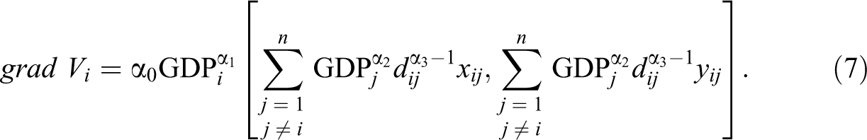
g r a d V_{i} = α_{0} {GDP}_{i}^{α_{1}} [\sum_{\begin{matrix} j = 1 \\ j \neq i \end{matrix}}^{n} {GDP}_{j}^{α_{2}} d_{i j}^{α_{3} - 1} x_{i j}, \sum_{\begin{matrix} j = 1 \\ j \neq i \end{matrix}}^{n} {GDP}_{j}^{α_{2}} d_{i j}^{α_{3} - 1} y_{i j}] .

The latter equation can be estimated in a stepwise way for identifying the gradient field of an export nation, starting off from the estimation of the underlying gravity model. On the basis of the estimate of the distance friction parameter (elasticity) $α_{3}$ , the potential V_i can be determined for the export country, so that the scalar field of potential can be estimated. Finally, the vector gradient field of the exporting area can be determined and geographically mapped out. More details and an extensive application can be found in Gornisiewicz, Nijkamp, and Ratajczak (2020). The latter modeling approach will now be employed for an illustrative application to the Dutch trade flows.

Gravity Potential Modeling of Dutch Trade Flows: An Example

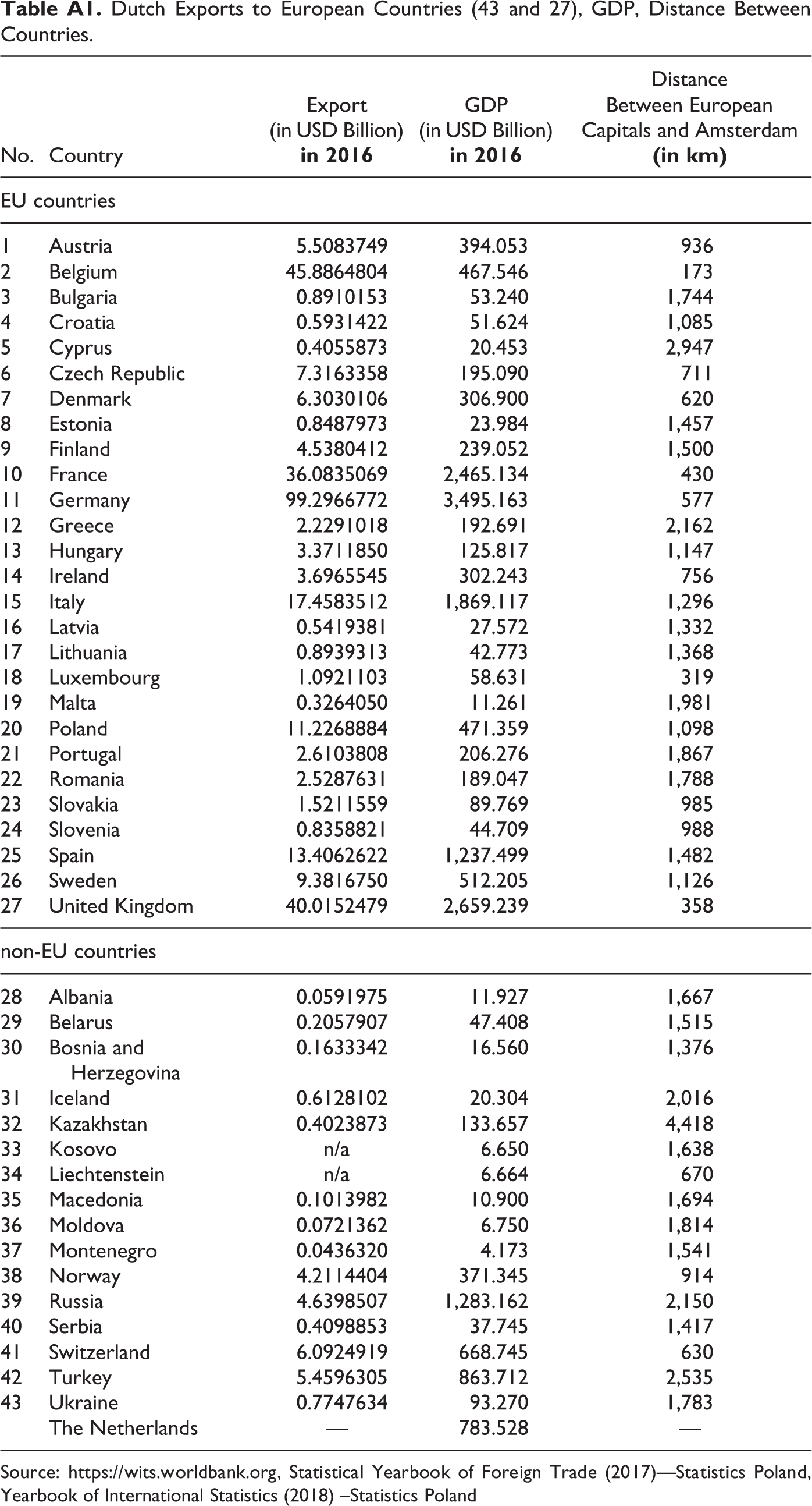
The main objective of the analysis presented here is the identification and assessment of gravity potential models of international trade with the simplest possible structure, with the aim of illustrating the way of constructing geographic potential model maps, and how to carry out a vector gradient analysis of trade flows. To this end, and for the sake of illustration, various data on Dutch exports will be used (see Appendix, Table A1).

A Potential-gradient Analysis of Dutch International Trade

The data included in Table A1 allow us to estimate by means of STATISTICA v.12.5 software the gravity-type models mapping out Dutch exports to European countries and, more narrowly, to the EU countries. The Netherlands is a well-developed state, with many trade interactions with other countries. It enjoys a relatively high GDP and exports regularly to various countries in the world. It is therefore plausible that gravity models depicting Dutch exports offer interesting mapping of spatial trade interactions.

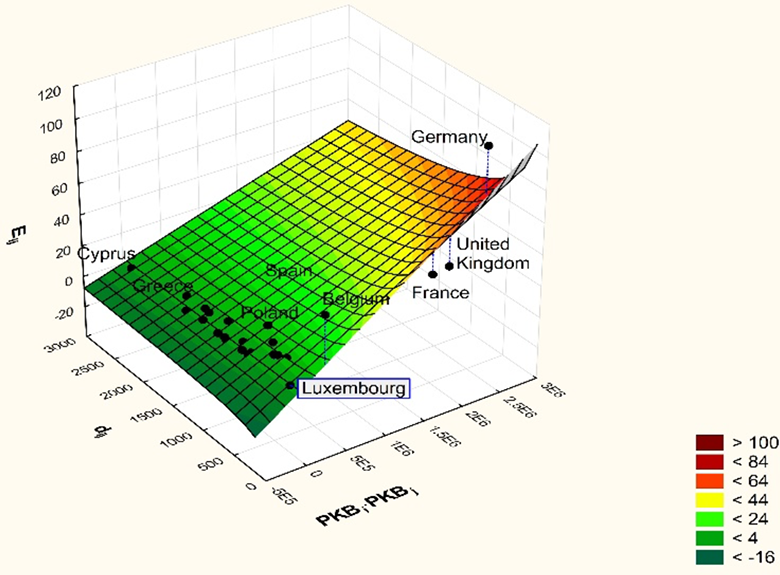
Application of the above mentioned non-linear estimation procedure allowed us to estimate the gravity model of exports of the Netherlands in the following form:

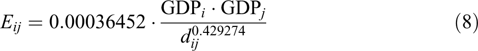
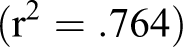
E_{i j} = 0.00036452 \cdot \frac{{GDP}_{i} \cdot {GDP}_{j}}{d_{i j}^{0.429274}}

(r^{2} = .764)

Its geometric form is presented in Figure 4. In model (8), the value of α₃ is below 1, which indicates that the Dutch exports are inelastic, i.e. they are not very sensitive to an increase in distance vis-a-vis the countries to which goods are exported.² This means that a decrease or increase in distance does not trigger off a change in exports from the Netherlands to other European countries. What would be a plausible explanation? Clearly, the generally recognized high quality of products exported from the Netherlands might provide some clarification for this stability in international trade patterns, but this ought to be further explored.

Figure 4.

Gravity model of Dutch exports to 43 European countries. Source: own compilation.

Interestingly, Figure 4 suggests that among all forty-five European countries, the Netherlands enjoys particularly intense trade with the neighboring countries like Germany, the UK and Belgium. These countries have also robus economies and are located relatively closely to the Netherlands. On the other hand, the concentration of the points in Figure 4, representing individual European countries along the line parallel to the $d_{i j}$ axis, illustrates the interesting situation when most European countries appear to trade with the Netherlands at a rather similar level of intensity. To draw a map of the export potential for the Netherlands, equation (5) was used, of course, with a specific adjustment for the value of α₃ equal to 0.429274. The surface of the potential is next depicted in Figure 5. The shape of the surface of the gravitational potential in Figure 5 highlights an interesting part of the European continent that is particularly involved in trade with the Netherlands. It also shows the prominent position of Germany and a crescent-shaped ridge extending from the Mediterranean (Italy) to the North Sea (Great Britain). These are the areas, not limited by political boundaries, with the greatest accessibility to Dutch exports.

Figure 5.

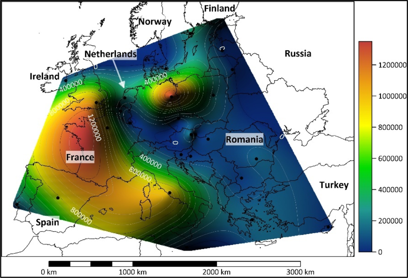
Potential map of Dutch exports to forty-three European countries. Source: own compilation

A Gradient Analysis of Dutch Exports to Forty-Three European Countries

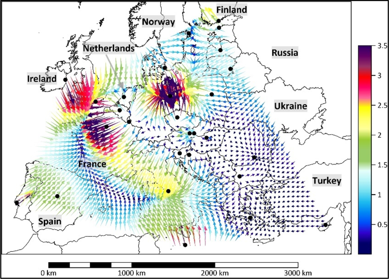
Notably, in an analysis of international trade, of importance is not only the size of trade exchange but also the direction of the exchange (in a geopolitical sense) and its intensity. Of course, the outcome depends on many factors among which (as numerous surveys confirm), the GDP is the most important. Figure 6 developed by using SUFER v.17 software shows both the directions and intensity of Dutch exports.

Figure 6.

Gradient full vectors of Dutch exports potential model (forty-three European countries). Source: own compilation.

The gradient vector field in Figure 6 not only magnifies the countries with which Dutch exports have the biggest volumes but also emphasizes the export’s macroscopic spatial structure. The arrangement of gradients appears to reflect the well-known European “blue banana” and reveals Germany’s special (leading) role in attracting Dutch exports.

Through the spatial distribution of vectors and their rank revealed in the form of changing colors, lengths and thicknesses, it is possible to determine the parts of the European continent where trade between the Netherlands and the countries in question is particularly intense. The vector system also allows to identify countries that, due to possible future changes in the rise of their GDP and given their distance to the Netherlands, might be able to alter the directions of cross-border trade (e.g. Ukraine, Romania, Balkan countries).

6.3. Dutch Exports to Twenty-Seven Countries of the European Union

In the next step of our empirical research, the countries under investigation were limited to the twenty-seven member states of the EU which play a key role in Europe’s economy. The gravitation model of Dutch exports was in this case estimated as follows:

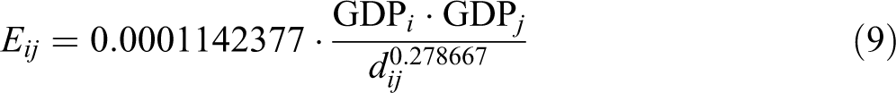
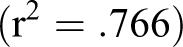
E_{i j} = 0.0001142377 \cdot \frac{{GDP}_{i} \cdot {GDP}_{j}}{d_{i j}^{0.278667}}

(r^{2} = .766)

Figure 7 is a geometric representation of this model.

Figure 7.

Gravity model of Dutch exports to EU members. Source: own compilation.

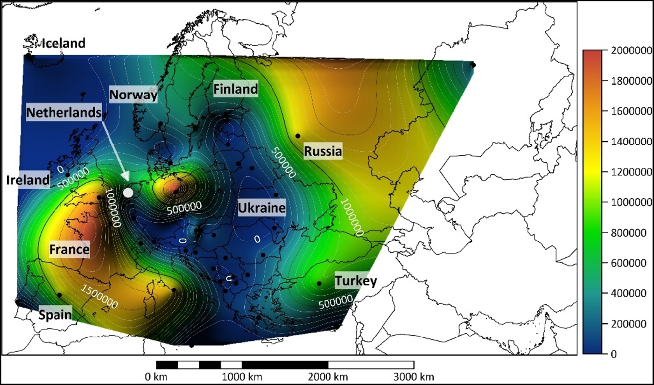
In model (9), the parameter α₃ is smaller than α₃ in model (8). This indicates that Dutch exports to the EU countries are even less elastic than in the case of exports to all the forty-three European countries. We can therefore assume that, when goods are exported to EU countries, the distance between countries does not play a critical role. Of key importance are other factors, such as for instance the aforementioned quality of products, political and social stability, advanced trade system, business, culture etc. The estimated parameters α₀ and α₃ from model (5) allowed us to depict the potential field of exports in the form of a map in Figure 8. The high values of the equipotential lines confirm that in the European space-economy, Dutch products are exported predominantly to the countries with the most robust economies due to their favorable trade accessibility in relation to their GDP.

Figure 8.

Potential map of Dutch exports to EU members. Source: own compilation.

A Gradient Analysis of Dutch Exports to the Twenty-Seven Countries of the European Union

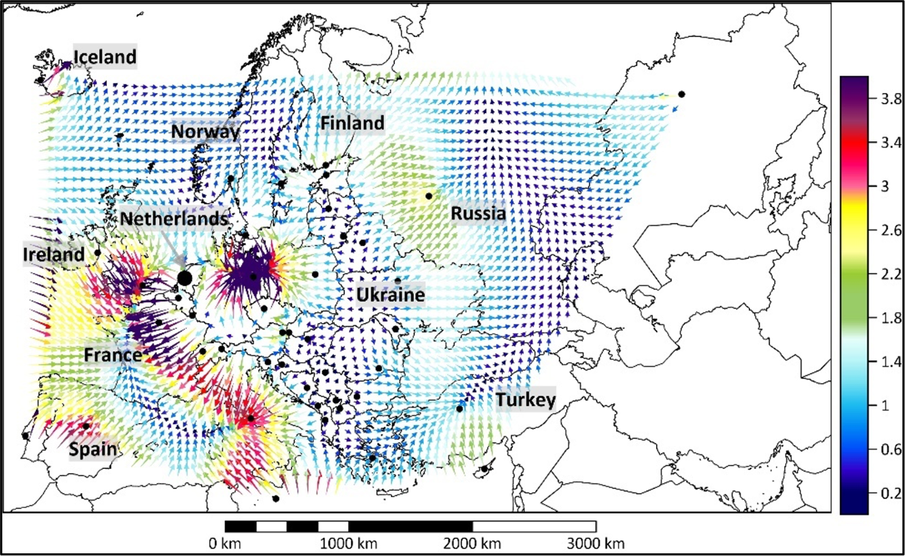
The gradient field in Figure 9 clearly confirms and reinforces the former conclusions. Obviously, the largest number of the longest vectors is located in countries with the highest GDP in Europe and, consequently, with dominant exports targeted at them. At the same time we should acknowledge the existence of vast areas with weak gradients covering the countries which accessed the EU relatively recently, i.e. economies weaker than the economies of the leading nations in the EU.

Figure 9.

Gradients full vectors of Dutch exports potential model (EU members). Source: own compilation.

Finally, there is a shortening and thinning out of a vector location in South-Eastern Europe. This is an indication that, in spatial terms, the Netherlands has an opportunity to increase its exports to countries like Romania, Bulgaria, Croatia, Slovakia, etc.

Conclusion

Providing an explanation for the complexity of spatial flows such as interregional or international trade flows poses a difficult scientific problem. Despite frequently voiced criticism, the gravity model in spatial economics has proven to be an effective research tool. Due to the fact that in this model, distance is one of the moderator variables, the gravity model also creates an opportunity for an in-depth spatial analysis. In the present study, the role of the power exponent of Newtonian distance has been highlighted, by providing the elasticity with a more economic-oriented interpretation. It seems possible that values above 1 reinforce the role of distance in trade exchange, while values below 1 reduce this role.

In the light of the results presented above it may be concluded that in general, the distance adversely affects spatial interactions and trade exchange between regions or countries with high revenues; the resistance of long-distance transport and trade exchange may weaken, but it still remains significant. A similar scenario appears to be present in trade between the OECD countries and states with Islam as the dominant religion.

It may also be concluded that the impact of globalization on overcoming the resistance of distance is particularly evident in countries with robust and stable economies. By means of a comprehensive analysis, Chaney (2013, 17) has proven that, in the case of direct interactions between trading companies and their suppliers and customers and when the companies’ sizes are well approximated by Zipf’s law, the aggregated trade volume is strictly proportional to the size of the country and inversely proportional to distance. Therefore, the elasticity equals –1. This is an indication that an increase in the distance between trade partners by 1% will result in a drop in trade exchange by exactly 1%. Therefore, the volume of exchange is neutral, but this only holds true for highly developed countries.

We have also found out that in the case of a highly developed country located among other highly developed countries, the elasticity may even drop below 0.5. This means that the role of distance in international trade exchange has been dramatically diminished. In our study, the Netherlands is a representative example in this context.

The methodology employed in this work needs a specific comment, which revolves around the theory of gravity potential and differential geometry. The heart of the matter here is extending the analysis of international trade with a purely spatial aspect by using the model of gravity potential. It allows to identify the economic potential (scalar) in any given place in geographic space. While potential models have a long history in economic geography (and have been largely neglected in conventional economics), to the best of our knowledge, they have not been applied in analyses of international trade. In literature on economics and geography, there have been no cases of employing gradient analysis where the starting point is the potential area. The gradient analysis used in our study has led to an in-depth spatial analysis of export flows in Europe. It has resulted in vector maps which make it possible to precisely identify the directions and areas (not only of countries) of the maximum export growth in the countries under scrutiny. This analysis may also be enriched by a procedure targeted at delimitation of areas of spatial divergence and convergence in the context of flows taking place in international trade.

Our spatial-economic trade study was inspired by gravitational principles in the context of spatial interaction modeling. It is also noteworthy that these principles apply analogously to other spatial economic research fields, where flows in a spatial network are determined by attraction forces of nodal points under conditions of (generalized) distance frictions. Vector gradients based on gravity potential models can therefore be applied also to transportation, migration, shopping or social interactions.

Finally, gravity theory models are increasingly relevant in the new framework of the “death of distance” hypothesis (see Tranos and Nijkamp 2013), in complex spatial network analysis (see Reggiani and Nijkamp 2006; Fischer and LeSage 2020) and in a new analysis framework based on complex network choice behavior, referred to as radiation (see Simini et al. 2012; Simini, Maritan, and Neda 2013; Varga, Toth, and Meda 2016). It is thus clear that gravitational analysis is a central and promising paradigm in modern spatial interaction analysis and will continue to attract the attention of regional scientists and spatial economists.

Footnotes

Appendix

Table A1.

Dutch Exports to European Countries (43 and 27), GDP, Distance Between Countries.

No.	Country	Export(in USD Billion) in 2016	GDP(in USD Billion) in 2016	Distance Between European Capitals and Amsterdam (in km)
EU countries
1	Austria	5.5083749	394.053	936
2	Belgium	45.8864804	467.546	173
3	Bulgaria	0.8910153	53.240	1,744
4	Croatia	0.5931422	51.624	1,085
5	Cyprus	0.4055873	20.453	2,947
6	Czech Republic	7.3163358	195.090	711
7	Denmark	6.3030106	306.900	620
8	Estonia	0.8487973	23.984	1,457
9	Finland	4.5380412	239.052	1,500
10	France	36.0835069	2,465.134	430
11	Germany	99.2966772	3,495.163	577
12	Greece	2.2291018	192.691	2,162
13	Hungary	3.3711850	125.817	1,147
14	Ireland	3.6965545	302.243	756
15	Italy	17.4583512	1,869.117	1,296
16	Latvia	0.5419381	27.572	1,332
17	Lithuania	0.8939313	42.773	1,368
18	Luxembourg	1.0921103	58.631	319
19	Malta	0.3264050	11.261	1,981
20	Poland	11.2268884	471.359	1,098
21	Portugal	2.6103808	206.276	1,867
22	Romania	2.5287631	189.047	1,788
23	Slovakia	1.5211559	89.769	985
24	Slovenia	0.8358821	44.709	988
25	Spain	13.4062622	1,237.499	1,482
26	Sweden	9.3816750	512.205	1,126
27	United Kingdom	40.0152479	2,659.239	358
non-EU countries
28	Albania	0.0591975	11.927	1,667
29	Belarus	0.2057907	47.408	1,515
30	Bosnia and Herzegovina	0.1633342	16.560	1,376
31	Iceland	0.6128102	20.304	2,016
32	Kazakhstan	0.4023873	133.657	4,418
33	Kosovo	n/a	6.650	1,638
34	Liechtenstein	n/a	6.664	670
35	Macedonia	0.1013982	10.900	1,694
36	Moldova	0.0721362	6.750	1,814
37	Montenegro	0.0436320	4.173	1,541
38	Norway	4.2114404	371.345	914
39	Russia	4.6398507	1,283.162	2,150
40	Serbia	0.4098853	37.745	1,417
41	Switzerland	6.0924919	668.745	630
42	Turkey	5.4596305	863.712	2,535
43	Ukraine	0.7747634	93.270	1,783
	The Netherlands	—	783.528	—

Source: https://wits.worldbank.org, Statistical Yearbook of Foreign Trade (2017)—Statistics Poland, Yearbook of International Statistics (2018) –Statistics Poland

Acknowledgments

Peter Nijkamp acknowledges the grant of the Romanian Ministry of Research and Innovation, CNCS—UEFISCDI, project number PN-III-P4-ID-PCCF-2016-0166, within the PNCDI III” project ReGrowEU -Advancing ground-breaking research in regional growth and development theories, through a resilience approach: toward a convergent, balanced and sustainable European Union (Iasi, Romania).

Declaration of Conflicting Interests

The author(s) declared no potential conflicts of interest with respect to the research, authorship, and/or publication of this article.

Funding

The author(s) disclosed receipt of the following financial support for the research, authorship, and/or publication of this article: Peter Nijkamp acknowledges a grant from the Romanian Ministry of Research and Innovation - CNCS-UEFISCDI, nr PN-III-P4-IDPCCF-2016-0166 ReGrowEU.

ORCID iD

Peter Nijkamp

Notes

References

Almog

Bird

Garlaschelli

. 2015. “Enhanced Gravity Model of Trade: Reconciling Macroeconomic and Network Models.” Frontiers in Physics 7:1–11.

Anderson

J. E.

2010a. “The Gravity Model.” NBER Working Paper No. 16576. NBER, Washington, DC.

Anderson

J. E.

2010b. “The Incidence of Gravity.” In The Gravity Model of International Trade, edited by van Bergeijk

P. A. G.

Brakman

, 71–87. Cambridge, MA: Cambridge University Press.

Anderson

J. E.

Van Wincoop

. 2003. “Gravity with Gravitas: A Solution to the Border Puzzle.” American Economic Review 93 (1): 170–92.

Anderson

J. E.

Yotov

Y. V.

. 2012. “Gold Standard Gravity.” NBER Working Paper No. 17825 . NBER, Washington, DC.

Anderson

T. R.

1956. “Potential Models and the Spatial Distribution of Population.” Papers in Regional Science 2 (1): 175–82.

Andersson

A. I.

Andersson

D. E.

. 2017. Time, Space and Capital. Cheltenham, UK: Edward Elgar.

Baldwin

R. E.

Wyplosz

. 2004. The Economics of European Integration. London, UK: McGraw-Hill.

Batty

1970. “Models and Projections of the Space Economy.” Town Planning Review 41:121–48.

10.

Batty

1976. Urban Modelling. Cambridge, MA: Cambridge University Press.

11.

Batty

Longley

. 1994. Fractal Cities. London, UK: Academic Press.

12.

Bergstrand

J. H.

1985. “The Gravity Equation in International Trade: Some Microeconomic Foundations and Empirical Evidence.” Review of Economics and Statistics 67 (3): 474–81.

13.

Bergstrand

J. H.

Egger

. 2010. “A General Equilibrium Theory for Estimating Gravity Equations of Billateral FDI, Final Goods Trade, and Intermediate Trade Flows.” In The Gravity Model of International Trade, edited by van Bergeijk

P. A. G.

Brakman

, 29–70. Cambridge, MA: Cambridge University Press.

14.

Beugelsdijk

de Groot

H. L. F.

van Schaik

A. B. T. M.

. 2004. “Trust and Economic Growth: A Robustness Analysis.” Oxford Economic Papers 56 (1): 118–34.

15.

Bröcker

1984. “How Do International Trade Patterns Affect Interregional Trade?” In Regional and Industrial Development Theories, Models and Empirical Evidence, edited by Andersson

A. C.

Isard

Puu

, 219–39. Amsterdam, the Netherlands: North-Holland.

16.

Bröcker

2020. “Spatial Interaction Models: A Broad Historical Perspective.” In Handbook of Regional Sceince, edited by Fischer

M. M.

Nijkamp

, 100–23. Berlin, Germany: Springer.

17.

Brun

Carrére

Guillaumont

De Melo

. 2005. “Has Distance Died? Evidence from a Panel Gravity Model.” The World Bank Economic Review 19 (1): 99–120.

18.

Cairncross

1997. The Death of Distance: How the Communications Revolution will Change our Lives. Boston, MA: Harvard Business School Press.

19.

Capello

Nijkamp

, Eds. 2020. Regional Growth and Development Theories. Cheltenham, UK: Edward Elgar.

20.

Caragliu

2015. “The Economics of Proximity.” PhD diss., VU University, Amsterdam, the Netherlands.

21.

Caragliu

Nijkamp

. 2012. “Cognitive Capital and Islands of Innovation.” Regional Studies 48 (4): 624–45.

22.

Carey

H. C.

1858. Principles of Social Science. Philadelphia, PA: J.B. Lippincott.

23.

Carrére

De Melo

Wilson

. 2009. “The Distance Effect and the Regionalization of the Trade of Low-income Countries.” CEPR Discussion Paper No. 7458 . CEPR, Washington, DC.

24.

Castanho

R. A.

Vulevic

Cabezas Fernandez

Fernandez-Pozo

Naranjo Gomez

J. M.

Loures

L. C.

. 2017. “Accessibility and Connectivity.” Sustainable Cities and Society 32:181–90.

25.

Chaney

2013. “The Gravity Equation in International Trade: An Explanation.” NBER working paper 19285 . NBER, Washington, DC.

26.

Chen

Y. G.

2008. “A Wave-spectrum Analysis of Urban Population Density.” Discrete Dynamics in Nature and Society 2008:article ID 728420.

27.

Chen

Y. G.

2009. “Urban Gravity Model Based on Ross-correlation Functions and Fourier Analyses of Spatio-temporal Processes.” Chaos, Solitons & Fractals 41 (2): 603–14.

28.

Chen

Y. G.

2012. “On the Four Types of Weight Functions for a Spatial Contiguity Matrix.” Letters in Spatial and Resource Sciences 5 (2): 65–72.

29.

Chen

Y. G.

2015. “The Distance-decay Function of Geographical Gravity Model: Power Law or Exponential Law?” Chaos, Solitons & Fractals 77:174–89.

30.

Chisholm

O’Sullivan

. 1973. Freight Flows and Spatial Aspects of the British Economy. Cambridge, MA: Cambridge University Press.

31.

Chojnicki

Czyz

Ratajczak

. 2011. Model Potencjalu (The Potential Model). Poznan: Bogucki Wydawnictwo Naukowe.

32.

Combes

P. P.

Lafourcade

Mayer

. 2005. “The Trade-creating Effects of Business and Social Networks.” Journal of International Economics 66:1–29.

33.

Converse

P. D.

1949. “New Laws of Retail Gravitation.” Journal of Marketing 14 (3): 379–84.

34.

Couclelis

2009. “Polyplexity: A Complexity Science for the Social and Policy Sciences.” In Complexity and Spatial Science, edited by Reggiani

Nijkamp

, 75–88. Berlin, Germany: Springer.

35.

Crafts

Venables

A. J.

. 2001. “Globalization in History. A Geographical Perspective.” In Globalization in Historical Perspective, edited by Bordo

Michael D.

Taylor

Alan M.

Williamson

Jeffrey G.

, 323–69. Chicago: University of Chicago Press.

36.

Deardorf

A. V.

1998. “Determinants of Bilateral Trade.” In The Regionalization of the World Economy, edited by Frankel

, 7–28. Chicago: University of Chicago Press.

37.

De Benedictis

Taglioni

. 2011. “The Gravity Model in International Trade.” In The Trade Impact on European Union Preferential Policies: An Analysis through Gravity Models, edited by De Benedictis

Berlin

L. Salvatici

, 1–21. Germany: Springer.

38.

Disdier

Head

. 2008. “The Puzzling Persistence of the Distance Effect on Bilateral Trade.” The Review of Economics and Statistics 90 (1): 37–48.

39.

Dixit

A. K.

Stiglitz

J. E.

. 1977. “Monopolistic Competition and Optimum Product Diversity.” American Economic Review 67:297–308.

40.

Eichengreen

Irwin

O. A.

. 1998. “Trade Blocs, Currency Blocks and the Re-oriented of the World Trade in the 1970’s.” Journal of International Economics 38:1–24.

41.

Fischer

M. M.

LeSage

J. P.

. 2020. “Network Dependence in Multi-indexed Data in International Trade Flows.” Journal of Spatial Econometrics 1 (4). doi: 10.1007/543071-02-00005-10.

42.

Foot

1987. “Spatial Interaction Modelling.” In Models in Urban Geography, edited by Yadav

C. S.

, 51–69. New Delhi: Concept Publishing.

43.

Fotheringham

A. S.

O’Kelly

M. E.

. 1989. Spatial Interaction Models: Formulations and Applications. Dordrecht, the Netherlands: Kluwer.

44.

Frankel

1997. Regional Trading, Blocs in the World Economic System. Washington, DC: Institute for International Economics.

45.

Fratianni

Kang

. 2006. “Heterogeneous Distance-elasticities in Trade Gravity Models.” Economics Letters 90:68–71.

46.

Friedman

T. L.

2005. The World is Flat: A Brief History of the Twenty-first Century. New York: Farrar, Straus and Giroux.

47.

Gornisiewicz

Nijkamp

Ratajczak

. 2020. “Gravity Modelling of Cross Border Trade Flows – A New Vector Gradient Approach.” In Szlakami Geografii Ekonomicznej, edited by Jagodzinski

Rakowski

, 433–49. Poznan: Bogucki Wydawnictwo Naukowe.

48.

Gould

1972. “Pedagogic Review of A.G. Wilson’s Entropy in Urban and Regional Modelling.” Annals of the Association of American Geographers 62 (4): 689–700.

49.

Guiso

Sapienzo

Zingales

. 2004. “Cultural Biares in Economic Exchange.” NBER Working Paper No. 11005, NBER, Cambridge, MA.

50.

Hagget

Cliff

A. D.

Frey

. 1977. Locational Analysis in Human Geography. London, UK: Arnold.

51.

Haynes

A. H.

1975. “Dimensional Analysis.” Geographical Analysis 7 (17): 51–68.

52.

Haynes

K. E.

Fotheringham

. 1984. Gravity and Spatial Interaction Models. Beverly Hills, CA: Sage.

53.

Head

Mayer

. 2010. “Illusory Border Effects, Distance Mismeasurment Inflated Estimates of Home bias in Trade.” In The Gravity Model of International Trade, edited by van Bergeijk

P. A. G.

Brakman

, 165–92. Cambridge, MA: Cambridge University Press.

54.

Head

Mayer

. 2014. “Gravity Equations: Workhorse, Toolkit, and Cookbook.” In Handbook of International Economics, volume 4, edited by Gopinath

Helpman

Rogoff

, 131–195. Amsterdam: Elsevier.

55.

Hutchinson

W. U.

2002. “Does Ease of Communication Increase Trade.” Scottish Journal of Political Economy 49:544–56.

56.

Ingram

D. R.

1971. “The Concept of Accessibility.” Regional Studies 5:101–07.

57.

Isard

1956. Location and the Space Economy. Cambridge, MA: MIT Press.

58.

Isard

1960. Methods of Regional Analysis. Cambridge, MA: MIT Press.

59.

Isard

McLaren

V. W.

. 1982. “Storia e Stato Attuale delle Richerche della Scienze Regionale.” In Problematiche dei Livelli Subregionali di Programmazione, edited by Bielli

La Bella

, 19–35. Milano: Franco Angeli.

60.

Janowski

(1908 [2013]). On Distances as a Factor of Cultural Development (English translation, 2013). Poznan: Bogucki Wydawnictwo Naukowe.

61.

Klaassen

L. H.

Wagenaar

Van der Weg

. 1972. “Measuring Psychological Distance between the Flemings and the Walloons.” Papers of the Regional Science Association 29:45–62.

62.

Kourtit

2016. “Super-proximity and Spatial Development.” Journal of Regional Research 36:215–31.

63.

Krugman

P. R.

1979. “Increasing Returns, Monopolistic Competition and International Trade.” Journal of International Economics 9:469–79.

64.

Krugman

P. R.

Obstfeld

. 2009. International Economics: Theory and Policy. Boston, MD: Pearson Addison-Wesley.

65.

Krynski

H. E.

1976. Matematyka dla Ekonomistów (Mathematics for Economists). Warszawa: PWN.

66.

Landkof

N. S.

1972. Foundations of Modern Potential Theory. Berlin, Germany: Springer.

67.

Linders

G. J.

2006. “Intangible Barriers to Trade.” PhD. diss., Tinbergen Institute, Amsterdam, the Netherlands.

68.

Linnemann

1966. An Econometric Study of International Trade Flows. Amsterdam, the Netherlands: North-Holland.

69.

Lukermann

Porter

P. W.

. 1960. “Gravity and Potential Models in Economic Geography.” Annals of the Association of American Geographers 50 (4): 493–504.

70.

Mantegna

R. N.

Stanley

H. E.

. 2000. Introduction to Econophysics. Cambridge, MA: Cambridge University Press.

71.

Mazurek

2016. “On Gravity Equation of Trade: A Case of Germany.” E+M Ekonomie a Management 19 (3): 20–30.

72.

McCalden

1975. “Macrogeographic Function.” Geographical Analysis 7:411–19.

73.

McCallum

1995. “National Borders Matter: Canada-U.S. Regional Trade Patterns.” The American Economic Review 85 (3): 615–23.

74.

Newton

(1686) 1999. The Principia: Mathematical Principles of Natural Philosophy. Los Angeles, CA: University of California Press.

75.

Niedercorn

J. H.

Bechdolt

H. V.

. 1969. “An Economic Derivation of the “Gravity Law” of Spatial Interaction.” Journal of Regional Science 9 (2): 273–83.

76.

Nijkamp

1975. “Reflections on Gravity and Entropy Models.” Regional Science and Urban Economics 5 (2): 203–25.

77.

Nijkamp

2021. “Borders as Opportunities in the Space-economy: Towards a Theory of Enabling Space.” Asian-Pacific Journal of Regional Science 5 (1): 223–39.

78.

Nijkamp

Reggiani

. 1992. Interaction, Evolution and Chaos in Space. Berlin, Germany: Springer.

79.

Östh

Lyhagen

Reggiani

. 2016. “A New Way of Determining Distance Decay Parameters in Spatial Interaction Models with Application to Job Accessibility Analysis in Sweden.” European Journal of Transport and Infrastructure Research 16 (2): 344–63.

80.

Poot

, Ed. 2004. On the Edge of the Global Economy. Cheltenham, UK: Edward Elgar.

81.

Rauch

J. E.

2001. “Business and Social Networks in International Trade.” Journal of International Economics 39:1177–203.

82.

Rauch

J. E.

Trindade

. 2002. “Ethnic Chinese Networks in International Trade.” Review of Economics and Statistics 84:116–30.

83.

Rautala

2015. Gravity Models of International Trade: Estimating the Elasticity of Distance with Finnish International Trade Flows . University of Eastern Finland http://epublications.uef.fi/pub/urn_nbn_fi_uef-20150356/urn_nbn_fi_uef-20150356.pdf.

84.

Ravenstein

E. G.

1885. “The Laws of Migration.” Journal of the Royal Statistical Society 49 (2): 167–235.

85.

Reggiani

Bucci

Russo

Haas

Nijkamp

. 2012. “Regional Labour Markets and Job Accessibility in City Network Systems in Germany.” Journal of Transport Geography 10:528–36.

86.

Reggiani

Nijkamp

, Eds. 2006. Spatial Dynamics, Networks and Modelling. Cheltenham, UK: Edward Elgar.

87.

Reilly

W. J.

1931. The Law of Retail Gravitation. New York: Knickerbocker Press.

88.

Romer

1994. “New Goods, Old Theory, and the Welfare Costs of Trade Restrictions.” Journal of Development Economics 43:5–38.

89.

Salas-Olmedo

M. H.

Garcia

Gutierrez

. 2015. “Accessibility and Transport Infrastructure Improvement Assessment.” Transportation Research A 82:110–29.

90.

Salvatici

2013. “The Gravity Model in International Trade.” AGRODEP Technical Note TN-04 . International Food Policy Research Institute, Washington, DC.

91.

Sen

Smith

T. E.

. 1995. Gravity Models of Spatial Interaction Behaviour. Berlin, Germany: Springer.

92.

Shepherd

. 2013. The Gravity Model of International Trade, A User Guide. United Nations ESCAP. http://www.unescap.org/resources/gravity-model-international-trade-user-guide.

93.

Sheppard

1979. “Geographic Potentials.” Annals of Association of American Geographers 69 (3): 438–47.

94.

Simini

Gonzalez

M. C.

Maritan

Barabasi

A. L.

. 2012. “A Universal Model for Mobility and Migration Patterns.” Nature 484:96.

95.

Simini

Maritan

Neda

. 2013. “Human Mobility in a Continuum Approach.” PLOS One 8 (3): e60069.

96.

Smith

1776. An Inquiry into the Nature and Causes of the Wealth of Nations. London, UK: Printed for W. Strahan; and T. Cadell.

97.

Snickars

Weibull

J. W.

. 1977. “A Minimum Information Principle.” Regional Science and Urban Economics 7 (1/2): 137–68.

98.

Squartini

Garlaschelli

. 2014. “Jan Tinbergen’s Legacy for Economic Networks: From the Gravity Model to Quantum Statistics.” In Econophysics of Agent-Based Models, edited by Aoyama

Chakrabarti

B. K.

Chakraborti

Ghosh

, 161–86. Springer.

99.

Starck

S. C.

2012. “The Theoretical Foundation of Gravity Modeling: What Are the Developments that have Brought Gravity Modeling into Mainstream Economics?” Master Thesis. Department of Economics, Copenhagen Business School, Copenhagen.

100.

Stewart

2002. Does God Play Dice? New York: Wiley-Blackwell.

101.

Stewart

J. Q.

1941. “An Inverse Distance Variation for Certain Social Influences.” Science 93:89–90.

102.

Stouffer

S. A.

1969. “Intervening Opportunities and Competing Migrants.” Journal of Regional Science 2:1–26.

103.

Theil

1967. Economics and Information Theory. Amsterdam, the Netherlands: North Holland.

104.

Tinbergen

1962. Shaping the World Economy. New York: Twentieth Century Fund.

105.

Tlustá

2015. “The Effect of Distance on International Trade: A Meta-analysis.” Bachelor thesis. Prague: Charles University in Prague.

106.

Torre

Wallet

, Eds. 2014. Regional Development and Proximity Relations. Cheltenham, UK: Edward Elgar.

107.

Tranos

Nijkamp

. 2013. “The Death of Distance Revisited: Cyber-place, Physical and Relational Proximities.” Journal of Regional Science 53 (5): 855–73.

108.

Varga

Toth

Meda

. 2016. “An Improved Radiation Model and Its Applicability for Understanding Commuting Patterns in Hungary.” Regional Statistics 6 (2): 27–38.

109.

Williamson

O. E.

1967. “Hierarchical Control and Optimum Firm Size.” Journal of Political Economy 75 (2): 123–38.

110.

Wilson

A. G.

1970. Entropy in Urban and Regional Modelling. London, UK: Pion.

111.

Wilson

A. G.

2000. Complex Spatial Systems. Singapore: Pearson Education.

112.

Wilson

A. G.

Bennett

R. J.

. 1985. Mathematical Methods in Human Geography and Planning. Chichester, UK: Wiley.

113.

Wilson

A. G.

Hawkins

A. T.

Hiu

G. J.

Wagon

D. J.

. 1969. “Calibration and Testing of the SELNIC Transport Model.” Regional Studies 3:337–50.

114.

K.-M.

2003. “Can Vertical Specialization Explain the Growth of World Trade?” Journal of Political Economy 111 (1): 52–102.

115.

Young

E. C.

1924. “The Movement of Farm Population, Ithaca, N.Y.” Cornell Agricultural Experiment Station Bulletin 426:14–36.

116.

Zielińska-Głębocka

2012. Współczesna gospodarka światowa, Przemiany, innowacje, kryzysy, rozwiązania regionalne (Contemporary International Economics). Warszawa: Oficyna a Wolters Kluwer Business.

117.

Zipf

G. K.

1949. Human Behaviour and the Principle of Least Effort. Cambridge, MA: Addison-Wesley.

Gravitational Analysis in Regional Science and Spatial Economics: A Vector Gradient Approach to Trade

Abstract

Keywords

Introduction

A Brief History of Gravity Analysis in Regional Science

Early Contributions

A New Wave of Interest

Social Physics

Gravitational Analysis in Spatial Economics

The Robustness of Distance-Friction Elasticities in Gravity Models: A Meta-Perspective

Gravity Potential Modeling: Scalar and Vector Analysis of Spatial Flows

Gravity Potential Model

5.2. The Gradient of Gravity Potential

Gravity Potential Modeling of Dutch Trade Flows: An Example

A Potential-gradient Analysis of Dutch International Trade

A Gradient Analysis of Dutch Exports to Forty-Three European Countries

6.3. Dutch Exports to Twenty-Seven Countries of the European Union

A Gradient Analysis of Dutch Exports to the Twenty-Seven Countries of the European Union

Conclusion

Footnotes

Appendix

Acknowledgments

Declaration of Conflicting Interests

Funding

ORCID iD

Notes

References