Sage Journals: Discover world-class research

Abstract

Categorizing places based on their network connections to other places in the region reveals not only population concentration but also economic dynamics that are missed in other typologies. The US Office of Management and Budget categorization of counties into metropolitan/micropolitan and central/outlying is widely seen as insufficient for many analytic purposes. In this article, we use a coreness index from network analysis to identify labor market centrality of a county. We use county-to-county commute flows, including internal commuting, to identify regional hierarchies. Indicators broken down by this typology reveal counterintuitive results in many cases. Not all strong core counties have large populations or high levels of urbanization. Employment in these strong core counties grew faster in the postrecession (2008–2015) than in other types of counties. This economic dimension is missed by other typologies, suggesting that our categorization may be useful for regional analysis and policy.

Keywords

urban and regional economic development economic growth and development policy and applications urban and regional spatial structure spatial structure network analysis spatial analysis methods labor force human resources population and employment distribution human spatial structure

Researchers and policy makers recognized that major cities are labor market centers that draw from their peripheral regions. For a while, states, local and federal agencies, counties, and other entities created their own ad hoc definitions of labor market areas based on these centers (Congressional Research Service 2014). In 1949, the US Office of Management and Budget (OMB) created a standard definition of these labor market areas based on commuting patterns and called them “standard metropolitan areas” (Klove 1952). The standardization of these areas enabled clearer communication between governments and public agencies. These definitions have been updated approximately once a decade since then. In 2015, the OMB delineated 945 core-based statistical areas (CBSAs) in the United States and Puerto Rico. Each of these CBSAs is collection of counties. Of these, 389 are metropolitan statistical area (MSA), with core areas of 50,000 or more people, and the rest are micropolitan statistical area (µSA), with core areas of 10,000 to 49,999 people.¹ For very large MSAs, such as New York, OMB has created metropolitan divisions that delineate smaller labor markets within the MSA (Congressional Research Service 2014).

OMB classifies two types of counties within the statistical areas: central, those counties that contain all or a substantial portion of the urbanized area; and outlying, those counties that have employment interchange measure with the central counties above 25 percent. In other words, the centrality of the county is defined by the urban population attributes of the county rather than its relative location in the commuting network. In 2015, a vast majority of the counties within CBSA are considered central; only 29 percent of the counties are peripheral/outlying (see Table 1). This is even more stark within µSAs where only 14 percent are considered peripheral. CBSAs are dominated by the central counties. They account for 92.5 percent of the CBSA population. These central counties are crucial to the delineation of these statistical regions and encompass the economic core of the country.

Table 1.

Types of CBSAs and Counties in Conterminous United States.

CBSA Type	County Type
CBSA Type	Central	Outlying	Total
MSA	725	436	1,161
µSA	560	94	654
Total	1,285	530	1,815

Source: Office of Management and Budget (2015).

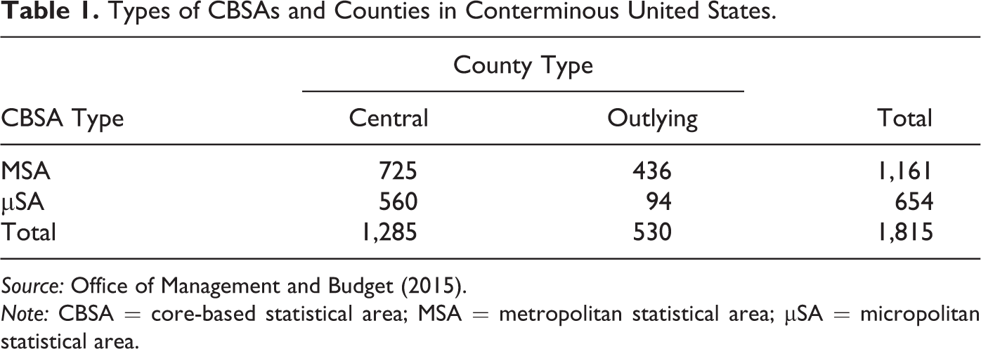
Note: CBSA = core-based statistical area; MSA = metropolitan statistical area; µSA = micropolitan statistical area.

While statistical areas are the most commonly used way of delineating labor market areas, several researchers have found the central/outlying/nonmetropolitan categorization to be too crude to describe the diversity of counties in the United States (e.g., Isserman 2005; Waldorf and Kim 2018; Wang et al. 2012). Many researchers have proposed their own typologies, though still based on commuting patterns or population levels, with the objective to better understand labor market areas (e.g., Fowler, Jensen, and Rhubart 2018; Han and Goetz 2019; Tolbert and Sizer 1996) or to better align public programs (e.g., Cook and Mizer 1994; De Lew 1992; Hewitt 1989; Lipscomb and Kashbrasiev 2008).

There is often a conflation of urbanicity with metropolitan areas. Isserman (2005) identified the differences between the US Census Bureau (2018) demarcation of urban and rural and OMB delineation of metropolitan and nonmetropolitan areas, even when they are frequently used interchangeably. The former is about separation of densely built from sparsely built places, while the latter is primarily about integration of residence and place-of-work. Consequently, OMB’s metropolitan areas include large swaths of rural lands, centered on urban counties. Nonetheless, the context of the metropolitan area becomes important feature for determination of the urbanity of a place. For example, the Economic Research Service (ERS 2013) of the US Department of Agriculture (USDA) created Rural–Urban Continuum Codes (RUCC) to distinguish counties based on the population size of the metro area and proximity to metro areas for a total of nine categories (three metro and six nonmetro). ERS has created a commuting rubric at the subcounty level as well. The rural–urban community area codes identify census tracts as metropolitan, micropolitan, or nonmetropolitan and break these down based on the size of the commute flow (ERS 2013). This ten-category classification system is more detailed both geographically and categorically but is still based in the OMB system. The National Center for Health Statistics (2014) created their own urban–rural typology of counties (four metro and two nonmetro) skewed toward metropolitan areas, by arguing that they stand in for urban and rural distinctions. These categories also include the distinctions between central and fringe counties in large metro regions and based on the size of the region (large, medium, and small). For example, Han and Goetz (2015) argue that resilience patterns are different across different types of counties. Using the economic recession of 2008 and the recovery pattern as evidenced by employment changes, they argue that counties with RUCC codes 1–5 (large population metro and nonmetro areas) have more resistance rather than resilience. Interestingly, an USDA report conflates rural with nonmetropolitan areas and argues that rural areas are slow to recover postrecession (Farrigan 2019). These concepts of centrality, urbanity, and proximity condition our understanding of disparities and challenges faced by different regions (e.g., Cutter, Ash, and Emrich 2016; Ingram and Franco 2012; Scala and Johnson 2017). While urbanity and proximity are important, we argue that they are complementary and not interchangeable with centrality.

In this article, we seek to establish a different notion of centrality based on the position of the county in a commuting network. We aim to uncover the regional structure by explicitly focusing on the network rather than node attributes (unlike OMB’s characterization of centrality). In particular, counties (or equivalents) that have small population (either because of constricted boundaries or because of a lack of residential lands) might still be destination areas for commuting. On the other hand, counties that have large populations may not necessarily have sufficient economic activity to justify the central designation. By focusing on the relationships among counties as a network, rather than the county attributes, we can begin to uncover some regional structures such as integration and core-periphery structures. The regions may be (multi) core based or comprise exclusively of peripheral nodes. Our aim is to demonstrate that such understanding complements our conventional understanding of centrality used in the literature and policy analysis. We also seek to demonstrate meso-level regional structure rather than intraregional spatial structure using a national analysis. We demonstrate that the positionality-based (as opposed to attribute based) centrality is correlated with economic growth and sectoral specialization. We also demonstrate that centrality is not correlated, in particular, with urbanity or population levels.

Network Analyses

Network analyses in regional science have a long history, though there have been significant divergences between geographers and network scientists (for an extensive literature review, see Ducruet and Beauguitte 2014). For example, Nystuen and Dacey (1961) use graph theory and commuting flows to identify regional hierarchies and nodal regions. Tong and Plane (2014) use spatial optimization techniques on the commuting network of all intercounty commuting linkages to identify clusters that rival OMB’s metropolitan area delineations. Nelson and Rae (2016) use community detection techniques to derive the megaregion structures. Using different community detection techniques and statistical inference, He et al. (2020) propose that there are multiple overlapping regions in the United States, hitherto unrecognized by the OMB or the other delineations such as megaregions. These are but a few examples of the use of graph theoretical analyses applied to regional science problems. Many of them rely on clustering of subgeographies to construct a larger geographical region. Among network science approaches in regional science, to our knowledge, very few have focused on centrality (see, e.g., Neal 2011; Sigler and Martinus 2016).

Centrality is a property of a node in a network indicating its relative importance (Degenne and Frose 1999). Many such measures of centrality have been proposed including degree centrality, betweenness centrality, and eigen centrality (e.g., Bonacich 1972; Freeman 1978). For a network with nodes and edges representing the connection between the nodes, a node degree is equal to the number of edges that are incident on the node (or conversely number of nodes it is connected to). A node with a higher degree is considered more central than ones with lower degree. However, degree centrality is a local measure, ignoring its importance in the overall network, through indirect connections. Betweenness centrality, a global measure, is based on how frequently a node appears on a path between two other nodes. While degree centrality is a measure of number of walks of length one that the node appears in, eigen centrality generalizes it to the number of walks of infinite length (Newman 2016). These centrality measures have been used to study many geographic networks such as transit systems (Derrible 2012), street networks (Agryzkov et al. 2019; Kirkley et al. 2018), knowledge networks (Maggioni and Uberti 2009), and global value chains (Cingolani, Panzarasa, and Tajoli 2017).

While these centrality measures are important characterizations of nodes, they are not always appropriate to understand the regional structure. In a commuting network among counties, betweenness centrality does not make intuitive sense. The degree centrality is a measure of how many commuters are incident on a county, while eigen centrality is about how well the county is connected to other central counties. While these two make some sense for commuting networks, they do not shed light on meso-level structural properties of the network. There is another concept called k-core centrality that relies on successive pruning of a network to identify more closely connected nodes (Seidman 1983). These concepts of identifying core and periphery of a network have found many applications ranging from airport commuting networks (Verma, Araújo, and Herrmann 2014) to gene regulatory networks (Narang et al. 2015). In this article, we focus on this measure.

Methods and Data

s-Core Decomposition of a Graph

A k-core of an unweighted simple binary graph is its subgraph where all the nodes have at least degree k (Dorogovtsev, Goltsev, and Mendes 2006; Seidman 1983). This subgraph is obtained by iteratively removing nodes from the network whose degree is less than k until a stable set of vertices with the minimum degree are reached. A node in a network has a coreness index k, if it belongs to a k-core but not a k + 1-core. Algorithms to calculate these indices quickly are proposed by Batagelj and Zaveršnik (2011).

This can be generalized to a directed network by focusing on the in-degree; that is, a k-core is the subgraph, where all nodes have an in-degree k. We can also generalize this concept to a weighted graph by using s-core decomposition, where degree of the vertex is replaced by strength of the vertices (Eidsaa and Almaas 2013). If, the edge weight between nodes i and j is denoted by a nonnegative w_ij, then the strength of the vertex i is defined as

s_{i} = \sum_{j \in N_{i}^{-}} w_{i j},

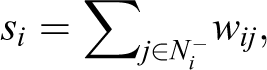
where $N_{i}^{-}$ is the in-neighborhood of i. The s-core is a subgraph where the nodes have at least strength s. As long as $w_{i j} \in ℤ^{+}$ , we can replace an edge in the graph with w_ij multiedges, and the decomposition of the graph by strength and degree are equivalent.

The s-core decomposition is illustrated in Figure 1 for a directed graph with multiple edges including loops. The entire graph in the figure is part of 0-core. Nodes A and F have in-degree 0 and therefore are not part of the 1-core of the graph (subgraph induced by nodes B, C, D, E, and G). Thus, the coreness of A and F is 0. In that 1-core of the subgraph, nodes D and G have in-degree 1. While they are not part of the 2-core of the graph, deleting them also renders B ineligible for 2-core. Thus, the coreness index of nodes B, D, and G is 1. This process continues, until all nodes are assigned a coreness index. We call this coreness index, the labor market centrality index (LMCI) when applied to commuting networks. LMCI is a dimensionless number. The absolute scale of LMCI is not important, as the counties in the upper decile of the index are characterized as strong core counties. The counties above the third quartile and below the upper decile are categorized as weak core, and counties below the third quartile are periphery. We then compare these categorizations to other conceptions of centrality and urbanity. To demonstrate the usefulness of this categorization, we use location quotients of different employment sectors and growth patterns to illustrate the differences. We use R (R Development Core Team 2017) and igraph package (Csardi and Nepusz 2006) for the analysis. We present the results using ggplot2 (Wickham 2016) and tmap (Tennekes 2018) packages.

Figure 1.

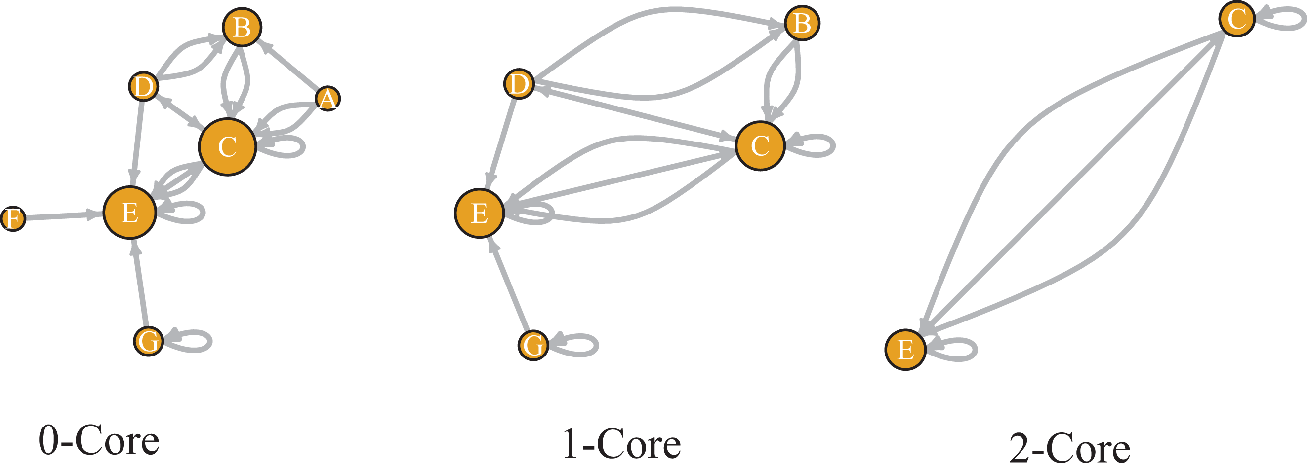
Illustration of network decomposition into core and periphery. Vertices are sized based on their in-degree.

Data

We use the 2011–2015 county-to-county commuting flow data from the American Community Survey (ACS) (US Census Bureau 2018). For the sake of exposition, we limit our analysis to the conterminous United States consisting of 3,109 counties. In this ACS data, 134,869 pairs of counties have nonzero commuters, representing 1.4 percent of the possible links. The network is relatively sparse, a testament to the continuing importance of geographic distance for labor market integration. These links represent 142.5 million commuters, of which 72 percent commuted within the same county. Using these data, we construct a directed network with self-loops, with counties as nodes. Two nodes (including the same node) are connected by an edge, if there are nonzero number of commuters from the residence county to workplace county. To simplify the computations, we scale the number of commuters logarithmically and use them as edge weights, a measure of strength of connection between the two counties.

Robustness Checks

Within county, commuters account for a substantial portion of the commuting in the United States. To test the effect of within commuting on the regional structure, we removed them and repeated the process described in s-Core Decomposition of a Graph section. Furthermore, because ACS is a survey rather than a census, each commuting value has an associated margin of error (MOE). The 90 percent confidence interval MOE for the commuting between two counties ranged from 1 to 8,301. To account for the impact of MOE on the LMCI, we draw a random number from a normal distribution with mean as the estimate of the number of commuters and standard deviation as MOE/1.65 for each pair of counties, truncating at 0. The distributions are assumed to be independent for pairs of counties. Using these random numbers as weights, we repeat the process (described in s-Core Decomposition of a Graph section) 1,000 times in a Monte Carlo simulation. To study the effect of the logarithmic transformation, we also use square root and linear transformation on the weights.

Results

The results point to tightly connected large cores in the Northeastern United States that span Boston to Washington, DC, in Florida around Miami and Tampa, in Southern California around Los Angeles, and in Northern California around San Francisco (see Figure 2A). As can be expected, there are also numerous other smaller cores around Miami, Atlanta, Chicago, Detroit, Seattle, Denver, and other cities. While it is tempting to conclude that core counties are counties with concentrated and large population, Figure 3 shows that at the upper tail of the distribution, there is substantial variation in population. The empirical cumulative distribution function plots reveal interesting patterns (see Figure 2B). The central counties in MSAs clearly have high LMCI compared to other types of counties. At the upper tail of the distribution, central MSA counties, the centrality index is not correlated with the population and is more reflective of the economic integration with the surrounding region (see Figure 3). The central μSA counties have much lower values than central MSA counties. However, some outlying MSA counties have higher index than central μSA (see Figure 2B).

Figure 2.

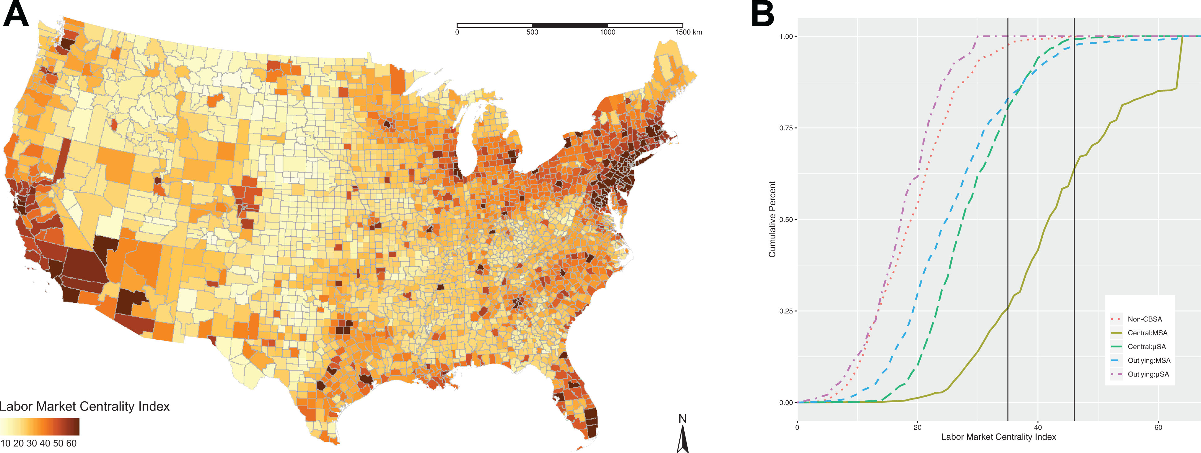
Distribution of the labor market centrality index based on the commuting network among counties in the conterminous United States. (A) Spatial distribution. (B) Empirical cumulative distribution by different types of counties defined by Office of Management and Budget.

Figure 3.

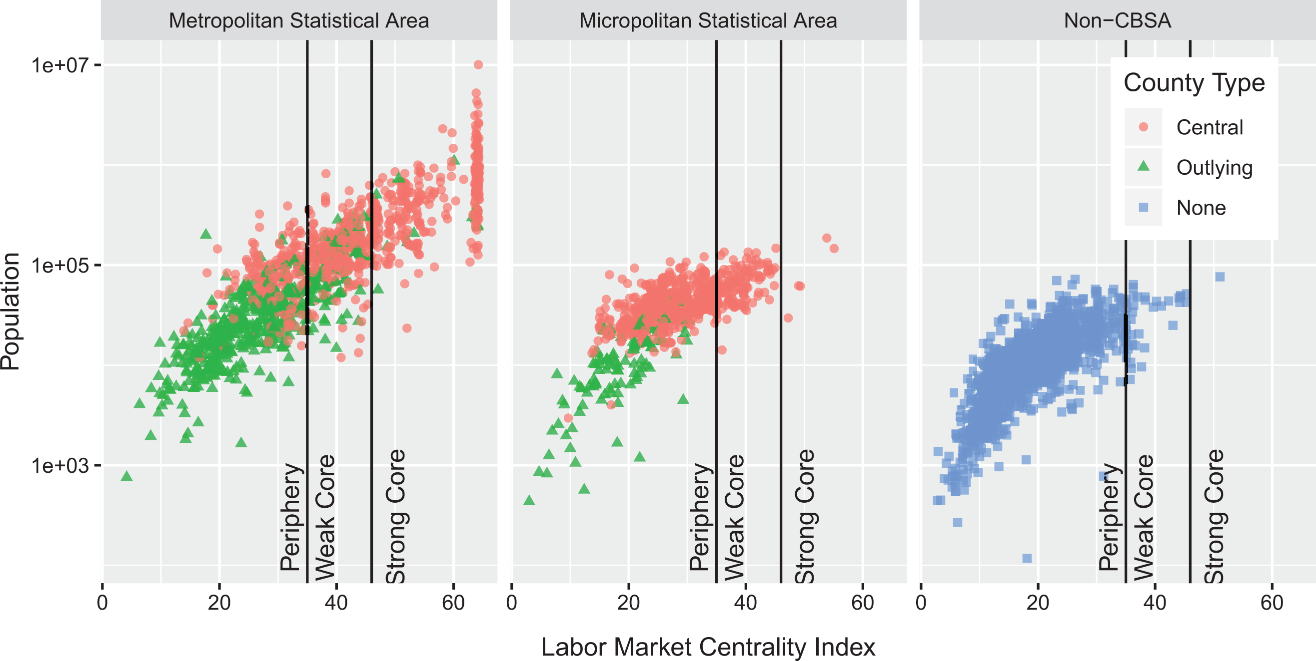
Labor market centrality index relative to the population of the county. County type is by Office of Management and Budget. Strong and weak core are defined by labor market centrality index cut at quantiles 0.9 and 0.75, respectively. Y-axis is logarithmically transformed for illustration.

There are 280 counties classified as strong core and 471 classified as weak core. The rest are in the periphery (see Figures 3 and 4). More importantly, many of the outlying μSA counties have lower index than non-CBSA counties (see Figure 2B). These unexpected results point to the need for closer examination of the classification that relies on node attributes. We need to rethink our understanding of the regional structure of the metropolitan USA and its relationship to the underlying labor market networks.

Figure 4.

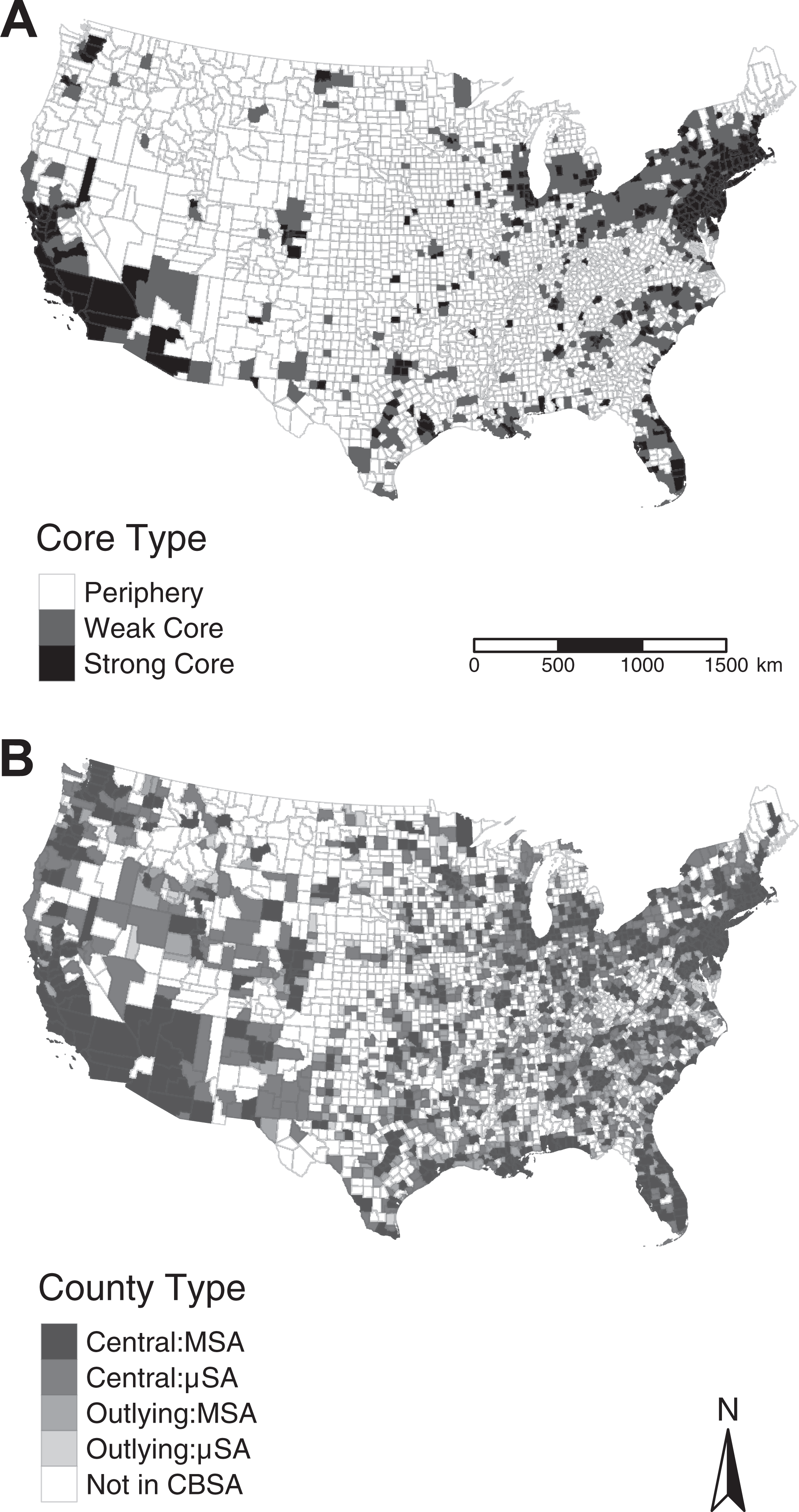
Comparing the spatial distributions of core and periphery using different definitions. (A) Results from the network analysis. Strong and weak core are defined by labor market centrality index cut at quantiles 0.9 and 0.75, respectively. (B) Office of Management and Budget categorizations of central and outlying counties in different core-based statistical area types.

Strong and Weak Core and Relationship to OMB Categorization

While it is tempting to conclude that core counties are counties with concentrated and large population, Figure 3 shows that at the upper tail of the distribution, there is substantial variation; that is, counties in the last index decile have population ranging from 23,000 (Fairfax city) to 10 million (Los Angeles County). Thus, the upper tail of the LMCI is not directly correlated with the population and is more reflective of the economic integration with the surrounding region. Within MSAs, many of the outlying counties (sixty-three) are part of the weak core, but fewer are in the strong core (eleven; see Figure 3). Of the 560 central counties in μSAs, 104 are classified as weak core and 5 are classified as strong core. These counties do not necessarily have large populations, but few of them are over 100,000 people (see Figure 3). There is one county (Sullivan, New York) that is not part any CBSA but belongs to a strong core. Similarly, two counties in New York, and one each in Connecticut, Pennsylvania, and North Dakota are part of μSAs, but are classified as strong core. Two such counties have more than 100,000 people. In contrast, there are no outlying counties in µSA that are a strong or weak core. Six MSA counties with less than 100,000 population are classified as strong core and ninety-eight as weak core.

In total, 638 central counties are not part of a strong or weak core. While these counties have urban populations above the CBSA thresholds specified, they have fewer commuters both to other nodes and to themselves, implying a comparatively weak local and regional economy. In general, the population of these peripheral counties is lower than core counties. However, it is not universally true; sixty-five counties (most of them MSA central counties) have more than 100,000 people are in the periphery. These disagreements in classifications provide a productive starting point to analyze the role of “small” nonurban counties in the regional economy and large urban counties that are experiencing economic stagnation and decline.

There are ninety-two distinct geographical clusters of strong core counties (defined by queen contiguity), with the biggest one comprising of 109 counties stretching from Portland, Maine to Northern Virginia. The second biggest cluster is the twenty-eight-county collection in California, from San Diego to Santa Rosa. The rest of the geographic clusters is comprised of one to seven counties, with 65 percent of them being a single county. With the inclusion of weak core counties, the number of geographic clusters increases to 108: twenty-three of the clusters are a collection of weak and strong core counties; forty-nine of the clusters are only comprised of weak core counties.

Robustness Checks and Uncertainty Estimates

When self-loops were removed, the indices with and without them for each county differ on average by 3.9 with a maximum of six and a minimum of two. The correlation coefficient between the indices with and without the loops is .99, implying that the main conclusions are not affected by the consideration of intracounty commuting. The categorizations of weak and strong cores are not affected.

In the Monte Carlo simulations accounting for the MOE in the commuting (described in Robustness Checks section), the indices of a county have a maximum range of fifteen and minimum of one, with an average of 6.7. The standard deviation, however, is small (<2.3). Counties with higher (though not large) variance in the LMCI are relatively sparsely populated, are near economic centers, and are more likely to be in the periphery, though there are some exceptions (e.g., Wake County in North Carolina and Duval County in Florida).

The precise monotonic transformation is largely irrelevant to main conclusions. While the main results are presented with log transformation of the number of commuters, we experimented with square root, linear transformations and recovered the main results but for the variations in rounding to integers. The categorization of weak and strong cores is not affected since the cuts are based on quantiles. The rounding to integers does not pose a major problem to the robustness of results as the estimates of commuters come with margins of error and the rounding errors are subsumed within them.

Discussion

We find that micropolitan areas are almost comprised of exclusively periphery counties, but metropolitan areas have a wide diversity. Similarly, other measures of urbanity show that places outside of urban areas are fairly consistently classified as periphery but counties with large populations or dense population are not necessarily strong core counties. This is because the LMCI captures economic aspects, mainly by using total commuting flows which is closely related to employment. Strong core counties tend to be those that have an expanding economy, regardless of population size.

Regional Structure of the Statistical Areas

Of the 378 MSAs, only thirty-eight contain all three types of counties and none of the µSA contains all three. In a substantial number of cases, MSAs contain exclusively one type of county; for example, fifty-six MSAs are exclusively strong core counties and seventy MSAs are exclusively comprised on periphery counties (see Table 2). Interestingly, five µSAs (Hudson, NY; Oneonta, NY; Pottsville, PA; Torrington, CT; and Williston, ND) comprise exclusively of strong core counties; 157 MSAs contained no counties that are periphery and 222 MSAs contained no strong core counties; 103 µSA have no periphery counties and 542 have no strong core. As mentioned before, one county that is not part of CBSA is considered a strong core, twenty-nine of them are weak core; a vast majority (97 percent) of the non-CBSA counties are peripheral counties.

Table 2.

Differences in the Structure of MSA and µSA based on Labor Market Centrality Index.

County Type	Number of MSA (378)				Number of µSA (547)
County Type	Exclusive	Combination (AND)			Exclusive	Combination (AND)
Periphery	70		77	88	439		5	0
Weak core	75	26	77		98	0	5
Strong core	56	26			5	0

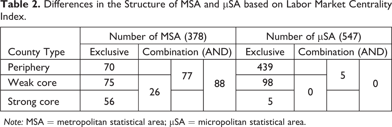
Note: MSA = metropolitan statistical area; µSA = micropolitan statistical area.

Strong core counties, on average, have higher number of both in, out, and within commuters in both MSA and µSA (see Figure 5). Within MSAs, there is marked difference in the in-commuters within central counties that are classified as strong core or periphery, while such stark difference is absent among the distributions of the commuters in the weak core and periphery counties. However, among the outlying counties, there are substantial differences in the commuters in periphery, weak core, and strong core counties in all types of commuters, with a clear gradation. These differences are noticeably absent in the µSAs.

Figure 5.

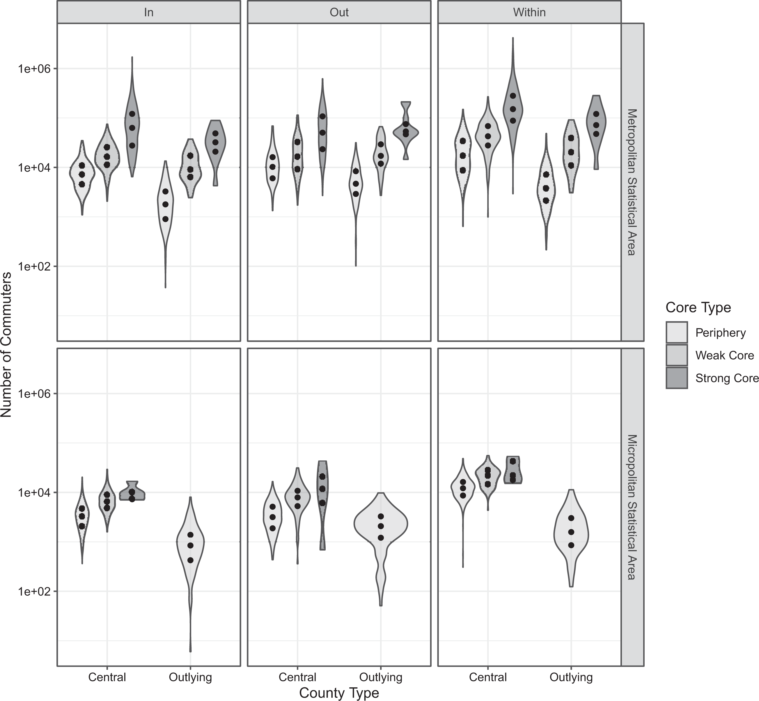
Patterns of commuting in different types of counties within core-based statistical areas. Violin plots represent the distributions while the interquartile range and the median are represented by points. Y-axis is logarithmically transformed for illustration.

Relationship of Coreness to Urbanity

Very few (twenty-nine) of the strong core counties have less than 250,000 people (see Table 3). However, the existence of large population does not make the county part of the core. In fact, there are as many counties with million plus people that are in the periphery as there are in the strong and weak cores. These are counties that are primarily residential counties that do not have strong economic attractors within them. Small counties (less than 250,000 population) with metro areas are far more likely to be in the periphery (223) than in the strong core (twenty-three), though there are some exceptions. Counties such as Litchfield, CT, and Schuykill, PA, have less than 250,000 people and are part of the strong core. On the other hand, Sullivan, NY, a strong core county with less than 80,000 population is not part of any CBSA region. There are six counties that RUCC classifies as nonmetro (categories four through nine) that LMCI identifies as strong core. The vast majority of nonmetro counties, however, is classified as periphery.

Table 3.

Contingency Table of Different Types of Classification of Counties based on Urbanity with the Core-periphery Classification.

County Type in Different Classification Schemes^a	Periphery	Weak Core	Strong Core
ERS Rural–Urban Continuum Code classification
Counties in metro areas of 1 million population or more	149	125	158
Counties in metro areas of 250,000 to 1 million population	187	95	93
Counties in metro areas of fewer than 250,000 population	212	118	23
Urban population of 20,000 or more, adjacent to a metro area	140	71	3
Urban population of 20,000 or more, not adjacent to a metro area	78	11	0
Urban population of 2,500 to 19,999, adjacent to a metro area	553	39	1
Urban population of 2,500 to 19,999, not adjacent to a metro area	414	9	2
Completely rural or less than 2,500 urban population, adjacent to a metro area	218	1	0
Completely rural or less than 2,500 urban population, not adjacent to a metro area	406	2	0
NCHS urban rural classification
Large central metro	0	0	68
Large fringe metro	149	128	91
Medium metro	187	91	91
Small metro	212	119	24
Micropolitan	528	104	5
Noncore	1,281	29	1

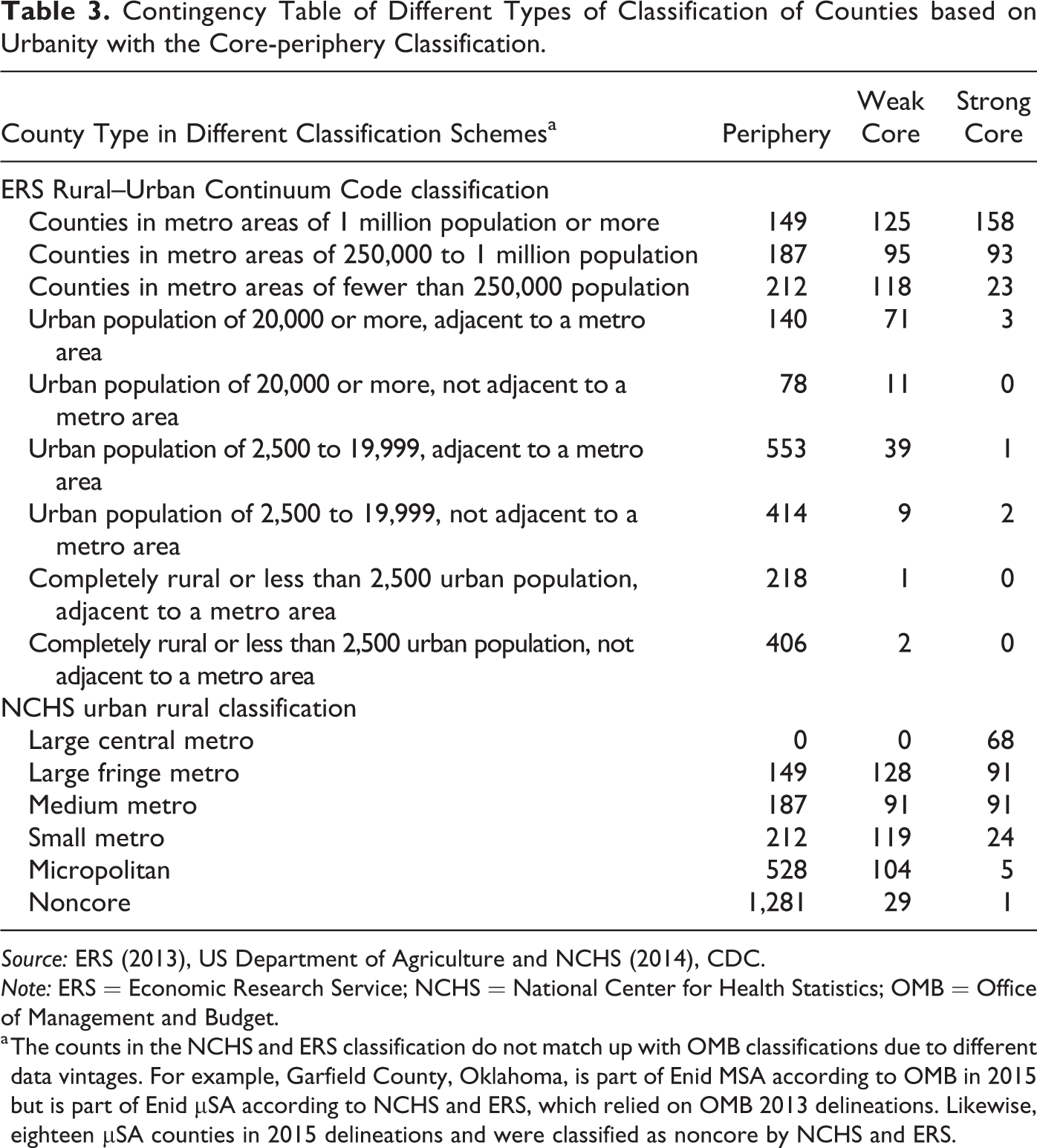
Source: ERS (2013), US Department of Agriculture and NCHS (2014), CDC.

Note: ERS = Economic Research Service; NCHS = National Center for Health Statistics; OMB = Office of Management and Budget.

^a The counts in the NCHS and ERS classification do not match up with OMB classifications due to different data vintages. For example, Garfield County, Oklahoma, is part of Enid MSA according to OMB in 2015 but is part of Enid µSA according to NCHS and ERS, which relied on OMB 2013 delineations. Likewise, eighteen µSA counties in 2015 delineations and were classified as noncore by NCHS and ERS.

Discretization might produce spurious relationships because of edge effects; therefore, it is useful to look at the underlying continuous variables. Waldorf and Kim (2018) fashion a continuous index of relative rurality (IRR) from zero (most urban) to one (most rural) based on population size, density, remoteness, and built-up area of a county. The Spearman’s correlation between IRR and the LMCI is −.88, suggesting that the more urban the county, the more likely it is a core county. However, closer examination suggests that much of this correlation is driven by rural counties with low LMCI values. At the top end of the LMCI and the lower end of the IRR (i.e., urban), there is substantial variance (see Figure 6).

Figure 6.

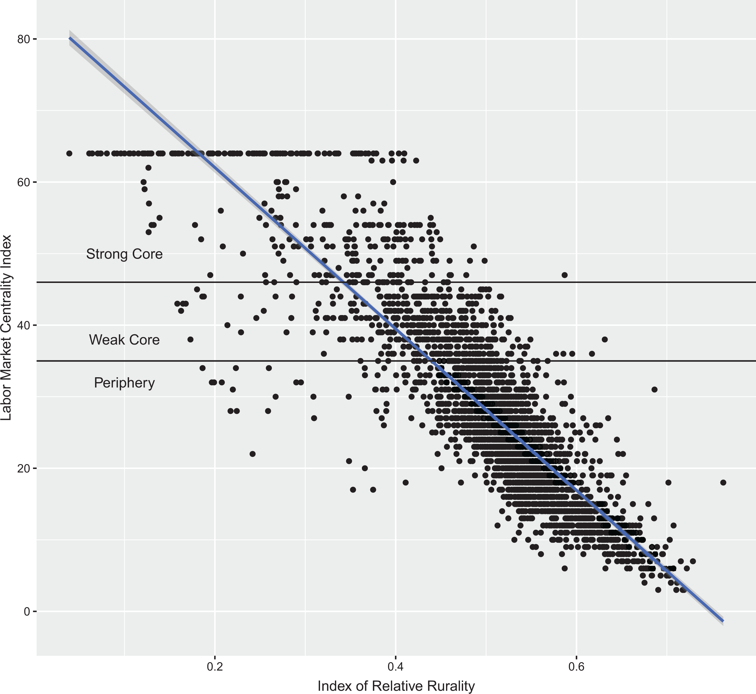
Relationship between labor market centrality index and index of relative rurality. Source: Waldorf and Kim (2018).

Economic Specialization of Core and Periphery

The previous measures indicate population size and density, but the LMCI reflects economic dimensions of the labor market. In counties with population over 250,000, there is a marked difference in the employment patterns. The median employment of strong core, weak core, and peripheral counties is around 0.365, 0.171, and 0.148 million, suggesting a strong economic differentiation. More crucially, the economic structure is also different among the different types of counties. On average, strong core counties have proportionally more private employment with median location quotient greater than 1 (see Table 4). Local government employment on the other hand is much higher in the periphery counties than in the strong core counties. Within private-sector employment, periphery counties and weak core, on average, specialize in goods producing industries, while the strong core counties specialize in service providing industries. Places with expanding economies tend to be more specialized in private employment instead of public employment, which can be thought of as subsistence employment: jobs that enable people to continue to live there. The US economy has expanded much more dramatically in the service sector over the past seventy years than in the goods-producing industries (Buera and Kaboski 2012). Strong core counties tend to be more specialized in services, while weak core and periphery counties have proportionately more jobs in goods-producing industries.

Table 4.

Employment Location Quotient by County Type.

County Type	Location Quotient
	Federal Government	State Government	Local Government	Private
	Federal Government	State Government	Local Government	Goods Producing	Service Providing
Periphery	.53 (.53)	.61 (.99)	1.74 (.98)	1.42 (.99)	0.75 (.22)
Weak core	.35 (.58)	.65 (.89)	1.15 (.48)	1.24 (.88)	0.9 (.19)
Strong core	.62 (.8)	.67 (.88)	0.9 (.37)	0.85 (.41)	1.02 (.14)

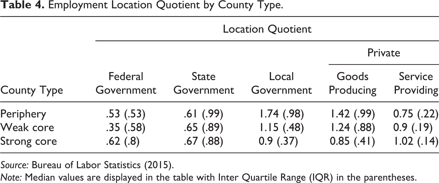
Source: Bureau of Labor Statistics (2015).

Note: Median values are displayed in the table with Inter Quartile Range (IQR) in the parentheses.

It is illustrative to see changes in the employment pre- and postrecession in different types of counties. While the weak core counties grew (in terms of number of jobs) roughly at the same rate as the strong core counties prerecession (2001–2008), the recovery in the postrecession has been twice as strong in the strong core counties in the postrecession (see Table 5). The recovery seems to have bypassed the periphery counties; while they grew at a healthy 3 percent before the recession, they contracted by 0.5 percent after the recession. In part, these numbers can be explained due the spatial sorting of specializations and the changing nature of the economy. However, these distinctions are not as stark, if we use the central and outlying distinctions of OMB. Central counties (on average) marginally grew faster compared to outlying counties (1.6 percent vs. 0.63 percent) during the postrecession, even while they had similar growth rates prerecession (6.75 percent vs. 6.45 percent). However, central counties with MSA significantly outpaced central counties within µSA in postrecession recovery (4.3 percent vs. −0.84 percent). This, together with the specialization in service industries indicates that it is not the population size of the county that is related to the economy but rather its place in the regional network. We do not make any claims as to the causal relationship between the position in the network and the economic growth.

Table 5.

Percent Change in Employment by County Type.

County Type	Employment Growth
County Type	2001–2008	2008–2015
Periphery	2.98 (12.73)	−0.52 (8.62)
Weak core	7.67 (16.95)	2.56 (10.1)
Strong core	7.52 (10.32)	5.05 (8.81)

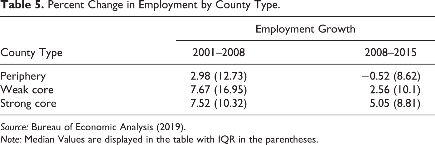
Source: Bureau of Economic Analysis (2019).

Note: Median Values are displayed in the table with IQR in the parentheses.

Limitations and Future Work

County as a unit of analysis in a commuting network may be useful for policy purposes, but microlevel regional structures of the commuting network can also be inferred using a finer geographic scale such as census tracts. However, at a census tract level, the MOE is substantial and Monte Carlo simulations take significant computational resources. Nevertheless, future work should understand the role of geographic scale in determining the centrality of places. Core periphery structure in tract-based commuting network can be used to extend and refine the work of He et al. (2020), who characterize the overlapping communities in a commuting network and distinguish between nodal and nonnodal clusters of counties. Such work is also a natural extension of Hartley, Kaza and Lester (2016) who identify the employment centers in a tract-based commuting network. It would be useful to identify whether these centers identified using McMillen (2001) correspond closely with the identified cores.

The LMCI has been calculated from ACS data that are primarily cross-sectional. Longer-term time trends in commuting patterns might be useful to more fully characterize the positionality of a node in a network. Other networks such as business transactions can supplement the information in commuting networks to get a more complete understanding of the place in the regional hierarchies.

Conclusion

There are many ways to understand human settlements. In this article, we looked at the regional structure from a network perspective. We found that how a county functions within the network of human settlement across the continental United States is based on population and economic activity. Our typology reflects economic dimensions in addition to population and density.

Metropolitan regions are formed around economic activity and therefore reflect economic centers, but existing typologies do not characterize the strength and nature of the regional economy well. Focusing on the role of the county in the network through commute patterns illuminates not just how central a county is in the labor market but also broadly demonstrates the strength of the economy. This is independent of the size of the population. Although there is some relationship between the size of the population and the size of the economy, there were some small counties with a lot of commute flows and large counties that had very little commuting.

Basing the index on total commuting rather than the number of commuters relative to the population of the sending county more closely mimics jobs and therefore reflects the character of the economy. Places with large populations but with little economic activity have a lower index. Rural places that may have a lot of internal commuting but not a lot of commuting from neighboring areas will also have a lower score. Places that have a lot of economic activity relative to the population size will score high because they not only have a lot of internal commuting but also a lot of in-commuting from surrounding counties.

This typology has the potential to be more dynamic than the OMB definition of metropolitan and micropolitan areas. Every time the OMB definitions are updated, there are changes to the delineations of metropolitan and micropolitan areas but those changes are mostly additive. Even regions in economic depressions do not lose their metropolitan status because the overall population continues to grow. By basing the typology on total commute flows, it reflects a region’s total economic activity and the connection between residents and that economic activity. In addition, our index categorizes counties into strong core, weak core, and periphery based on the score relative to other counties.

Categorizing counties based on their function in the network of human settlements is a useful way to understand the integration of population and economy. It shares some similarities with other typologies focused on commuting flows. However, it has the unique feature of reflecting the economic strength of the region in a more dynamic way than other categorizations and indices.

Footnotes

Declaration of Conflicting Interests

The author(s) declared no potential conflicts of interest with respect to the research, authorship, and/or publication of this article.

Funding

The author(s) received no financial support for the research, authorship, and/or publication of this article.

ORCID iD

Nikhil Kaza

Note

References

Agryzkov

Taras

Tortosa

Leandro

Vicent

José F.

Wilson

Richard

. 2019. “A Centrality Measure for Urban Networks based on the Eigenvector Centrality Concept.” Environment and Planning B: Urban Analytics and City Science 46 (4): 668–89.

Batagelj

Vladimir

Zaveršnik

Matjaž

. 2011. “Fast Algorithms for Determining (Generalized) Core Groups in Social Networks.” Advances in Data Analysis and Classification 5 (2): 129–45.

Bonacich

Phillip

. 1972. “Factoring and Weighting Approaches to Status Scores and Clique Identification.” Journal of Mathematical Sociology 2 (1): 113–20.

Buera

Francisco J.

Kaboski

Joseph P.

. 2012. “The Rise of the Service Economy.” American Economic Review 102 (6): 2540–69. https://doi.org/10.1257/aer.102.6.2540.

Bureau of Labor Statistics. 2015. QCEW Data Files. U.S. Bureau of Labor Statistics. Accessed December 30, 2019. https://www.bls.gov/cew/downloadable-data-files.htm.

Cingolani

Isabella

Panzarasa

Pietro

Tajoli

Lucia

. 2017. “Countries’ Positions in the International Global Value Networks: Centrality and Economic Performance.” Applied Network Science 2 (1): 21.

Congressional Research Service. 2014. Metropolitan Area Designations by OMB: History, 2010 Standards, and Uses. Washington, DC: CRS Report. Accessed July 30, 2019. https://www.everycrsreport.com/files/20140606_R42005_cc88d5c754b797d095e0880142d7c28aa739d871.pdf.

Cook

Peggy J.

Mizer

Karen

. 1994. ERS Typology Revised and Updated. Washington, DC: US Department of Agriculture. Rural Development Research Report. Accessed July 4, 2019. https://naldc.nal.usda.gov/download/CAT10829253/PDF.

Csardi

Gabor

Nepusz

Tamas

. 2006. “The Igraph Software Package for Complex Network Research.” InterJournal Complex Systems:1695.

10.

Cutter

Susan L.

Ash

Kevin D.

Emrich

Christopher T.

. 2016 “Urban-rural Differences in Disaster Resilience.” Annals of the American Association of Geographers. Accessed November 19, 2019. https://www.tandfonline.com/doi/abs/10.1080/24694452.2016.1194740.

11.

Degenne

Alain

Frose

Michel

. 1999. Introducing Social Networks, 1st ed. Thousand Oaks, CA: Sage.

12.

De Lew

Nancy

. 1992. “Geographic Classification of Hospitals: Alternative Labor Market Areas.” Health Care Financing Review 14 (2): 49–58.

13.

Derrible

Sybil

. 2012. “Network Centrality of Metro Systems.” PLoS One 7 (7): e40575.

14.

Dorogovtsev

S. N.

Goltsev

A. V.

Mendes

J. F. F.

. 2006. “K-core Organization of Complex Networks.” Physical Review Letters 96 (4). Accessed March 18, 2019. http://arxiv.org/abs/cond-mat/0509102.

15.

Ducruet

César

Beauguitte

Laurent

. 2014. “Spatial Science and Network Science: Review and Outcomes of a Complex Relationship.” Networks and Spatial Economics 14 (3): 297–316.

16.

Eidsaa

Marius

Almaas

Eivind

. 2013. “s-core Network Decomposition: A Generalization of k-core Analysis to Weighted Networks.” Physical Review E 88 (6): 062819.

17.

ERS (Economic Research Service). 2013. “Rural-urban Continuum Codes.” Accessed November 18, 2019. https://www.ers.usda.gov/data-products/rural-urban-continuum-codes/documentation/.

18.

Farrigan

Tracy

. 2019. “Rural Employment and Unemployment.” Accessed April 27, 2020. https://www.ers.usda.gov/topics/rural-economy-population/employment-education/rural-employment-and-unemployment/.

19.

Fowler

Christopher S.

Jensen

Leif

Rhubart

Danielle

. 2018. “Assessing U.S. Labor Market Delineations for Containment, Economic Core, and Wage Correlation.” https://doi.org/10.17605/OSF.IO/T4HPU.

20.

Freeman

Linton C.

1978. “Centrality in Social Networks Conceptual Clarification.” Social Networks 1 (3): 215–39.

21.

Han

Yicheol

Goetz

Stephan J.

. 2015. “The Economic Resilience of U.S. Counties during the Great Recession.” Review of Regional Studies 45 (2): 131–49.

22.

Han

Yicheol

Goetz

Stephan J.

. 2019. “Overlapping Labour Market Areas based on Link Communities.” Papers in Regional Science 98 (1): 539–53.

23.

Hartley

D. A.

Kaza

William Lester

. 2016. “Are America’s Inner Cities Competitive? Evidence from the 2000s.” Economic Development Quarterly 30 (2): 137–58.

24.

Mark

Glasser

Pritchard

Bhamidi

Kaza

. 2020. “Demarcating Geographic Regions Using Community Detection in Commuting Networks.” PLoS One 15 (4): e0230941.

25.

Hewitt

Maria

. 1989. Defining “Rural” Areas: Impact on Health Care Policy and Research. Washington, DC: US Congress. Staff Paper. Accessed June 30, 2019. http://govinfo.library.unt.edu/ota/Ota_2/DATA/1989/8912.PDF.

26.

Ingram

D. D.

Franco

S. J.

. 2012. “NCHS Urban-rural Classification Scheme for Counties.” Vital and Health Statistics. Series 2, Data Evaluation and Methods Research 154:1–65.

27.

Isserman

A. M.

2005. “In the National Interest: Defining Rural and Urban Correctly in Research and Public Policy.” International Regional Science Review 28 (4): 465–99.

28.

Kirkley

Alec

Barbosa

Hugo

Barthelemy

Marc

Ghoshal

Gourab

. 2018. “From the Betweenness Centrality in Street Networks to Structural Invariants in Random Planar Graphs.” Nature Communications 9 (1): 1–12.

29.

Klove

Robert C.

1952. “The Definition of Standard Metropolitan Areas.” Economic Geography 28 (2): 95–104.

30.

Lipscomb

C. A.

Kashbrasiev

R. V.

. 2008. “County Typologies to Inform Job Tax Credit Policy in Georgia—ProQuest.” Review of Regional Studies 38 (2): 233–50.

31.

Maggioni

Mario A.

Uberti

Teodora Erika

. 2009. “Knowledge Networks across Europe: Which Distance Matters?” The Annals of Regional Science 43 (3): 691–720.

32.

McMillen

Daniel P.

2001. “Nonparametric Employment Subcenter Identification.” Journal of Urban Economics 50 (3): 448–73.

33.

Narang

Vipin

Azfar Ramli

Muhamad

Singhal

Amit

Kumar

Pavanish

de Libero

Gennaro

Poidinger

Michael

Monterola

Christopher

. 2015. “Automated Identification of Core Regulatory Genes in Human Gene Regulatory Networks.” PLoS Computational Biology 11 (9): e1004504.

34.

NCHS (National Center for Health Statistics). 2014. 2013 NCHS Urban-rural Classification Scheme for Counties. Data Evaluation and Methods Research. Hyattsville, MD: Centers for Disease Control, US Department of Health and Human Services. Accessed November 18, 2019. https://www.cdc.gov/nchs/data/series/sr_02/sr02_166.pdf.

35.

Neal

Zachary

. 2011. “Differentiating Centrality and Power in the World City Network.” Urban Studies 48:2733–48.

36.

Nelson

Garrett Dash

Rae

Alasdair

. 2016. “An Economic Geography of the United States: From Commutes to Megaregions.” PLOS One 11 (11): e0166083.

37.

Newman

M. E. J

. 2016. “Mathematics of Networks.” In The New Palgrave Dictionary of Economics, 1–8. London, UK: Palgrave Macmillan. Accessed November 19, 2019. https://doi.org/10.1057/978-1-349-95121-5_2565-1.

38.

Nystuen

John D.

Dacey

Michael F.

. 1961. “A Graph Theory Interpretation of Nodal Regions.” Papers of the Regional Science Association 7 (1): 29–42.

39.

Office of Management and Budget. 2015. “Revised Delineations of Metropolitan Statistical Areas, Micropolitan Statistical Areas, and Combined Statistical Areas, and Guidance on Uses of the Delineations of These Areas.” OMB Bulletin 15–01. Washington, D. C. Accessed July 28, 2019. https://obamawhitehouse.archives.gov/sites/default/files/omb/bulletins/2015/15-01.pdf.

40.

R Development Core Team. 2017. “R: A Language and Environment for Statistical Computing.” Vienna, Austria. http://www.R-project.org.

41.

Scala

Dante J.

Johnson

Kenneth M.

. 2017. “Political Polarization along the Rural-urban Continuum? The Geography of the Presidential Vote, 2000–2016.” The ANNALS of the American Academy of Political and Social Science. Accessed November 19, 2019. http://journals.sagepub.com/doi/full/10.1177/0002716217712696.

42.

Seidman

Stephen B.

1983. “Network Structure and Minimum Degree.” Social Networks 5 (3): 269–87.

43.

Sigler

Thomas

Martinus

Kirsten

. 2016. “Extending beyond “World Cities” in World City Network (WCN) Research: Urban Positionality and Economic Linkages through the Australia-Based Corporate Network.” Environment and Planning A 49 (12): 2859–77.

44.

Tennekes

Martijn

. 2018. “tmap: Thematic Maps in R.” Journal of Statistical Software 84 (6): 1–39.

45.

Tolbert

Charles M.

Sizer

Molly

. 1996. US Commuting Zones and Labor Market Areas: A 1990 Update. Washington, DC: Rural Economy Division, Economic Research Service, US Department of Agriculture. Accessed January 30, 2014. https://usa.ipums.org/usa/resources/volii/cmz90.pdf.

46.

Tong

Daoqin

Plane

David A.

. 2014. “A New Spatial Optimization Perspective on the Delineation of Metropolitan and Micropolitan Statistical Areas.” Geographical Analysis 46 (3): 230–49.

47.

US Census Bureau. 2018. “2011–2015 5-year American Community Survey Commuting Flows.” Accessed March 17, 2019. https://www.census.gov/data/tables/2015/demo/metro-micro/commuting-flows-2015.html.

48.

Verma

Araújo

N. a. M.

Herrmann

H. J.

. 2014. “Revealing the Structure of the World Airline Network.” Scientific Reports 4:5638.

49.

Waldorf

Brigitte

Kim

Ayoung

. 2018. “The Index of Relative Rurality (IRR): US County Data for 2000 and 2010.” Accessed June 28, 2019. https://purr.purdue.edu/publications/2960/1.

50.

Wang

Man

Kleit

Rachel Garshick

Cover

Jane