Sage Journals: Discover world-class research

Abstract

Building on prior results that financial analysts have an information advantage relative to managers at the macroeconomic level, we show that such an information advantage is an important source of what managers learn from analysts in making investment decisions. Specifically, the sensitivity of corporate capital investment to analyst forecasts of firm earnings or long-term growth is positively associated with the exposure of a firm’s operations to macroeconomic factors, including the business cycle and energy prices. This effect is concentrated among firms whose analysts have greater macro-level insights or firms that have higher capital intensity and hence stronger incentives to learn. Overall, our results suggest that managers learn from analysts regarding the implications of macroeconomic factors for firm-specific prospects and incorporate what they learn into their capital investment decisions.

Keywords

capital investment managerial learning analyst forecasts macroeconomic information

Introduction

In making corporate investment decisions, managers face substantial uncertainties—the payoffs being dependent on macro-, industry-, and firm-level factors (Ferracuti & Stubben, 2019; Roychowdhury et al., 2019)—and therefore have incentives to learn about these factors from other market participants who possess information that managers do not have. Research has shown that the capital markets have a remarkable ability to aggregate information that generates predictions about real variables (Hayek, 1945) and that managers learn from such information when making investment decisions (e.g., Chen et al., 2007; Edmans et al., 2017; Foucault & Frésard, 2014; Jayaraman & Wu 2020; Luo, 2005).

However, given that managers are well-informed about their own firms, it remains unclear what specific information they seek to learn from the capital market and what types of market participants possess this specific information that induces managerial learning. Answers to these questions are important for our understanding of (a) the implications of relative information advantage between managers and outsiders and (b) the decision process for capital investments in the real economy.

We hypothesize that managers making capital investments learn from an important market intermediary, financial analysts, about the implications of macroeconomic factors for firm-specific prospects (the “managerial learning hypothesis”).¹ Studies show that analysts specialize in processing information not only at the firm level but also at the industry or macro-level (Hugon et al., 2016; Piotroski & Roulstone, 2004). In particular, Hutton et al. (2012) show that analysts are better than managers at predicting the implications of macroeconomic factors (specifically the business cycle, as proxied by gross domestic product or GDP, and energy prices) for firm performance and prospects. Importantly, it is not only analysts’ access to macro-level information, but also their superior ability to predict what it will mean for a given firm’s prospects, that affords them an information advantage.

Managers, given their primary focus on firm operations, have less access to macro-level information and less expertise in analyzing its implications for their firms (Hutton et al., 2012; Piotroski & Roulstone, 2004 ). Indeed, Anilowski et al. (2007) show that managerial guidance lags macroeconomic news, and Kim et al. (2016) document that high macroeconomic uncertainty decreases the likelihood of managers issuing forecasts, suggesting that they find it challenging to predict the implications of macroeconomic uncertainties for their firms. These results, together with those in Hutton et al. (2012), suggest that analysts have an information advantage relative to managers on firm-specific implications of macroeconomic factors, which are particularly relevant to a firm’s long-term strategy and growth. We therefore expect managers to learn from analysts regarding such implications when making investment decisions.

We note that although research shows that managers learn from stock prices, analysts can still play an incremental role in managerial learning for several reasons. First, even if the stock market is efficient in strong form, managers may require specific types or dimensions of investment-relevant information that are difficult and costly to extract from stock prices. Second, stock prices contain noise from sources such as noise traders and liquidity shocks. Dessaint et al. (2019) show that managers have difficulty filtering out such noise when using stock prices as signals about investment opportunities. For these reasons, managers have incentives to learn from alternative information sources or to attach a higher weight to information sources that can provide more direct implications for capital investments but are less prone to these types of noise. Consistent with this conjecture, prior research has shown that managers do learn from sources other than stock prices, such as peer firms’ Management discussion and analysis (MD&A) (Durnev & Mangen, 2020), in making capital investment decisions.

It is important to note, however, that capital investments are long term in nature, and managers may pay limited attention to the short-term ups and downs of macro factors in making long-term capital investment decisions. Furthermore, if managers do not recognize that analysts have information advantages on macroeconomic factors, or if managers are overconfident and ignore the private information in analyst forecasts, their investment decisions will be unaffected by analysts’ information advantages on macroeconomic factors. Overall, whether managers directly learn from analysts on macroeconomic factors is an empirical question.

We use revisions in analyst consensus earnings forecasts for the next year and analyst consensus long-term growth forecasts to capture analyst information. To document managerial learning from analysts on macro-related information, we adopt an approach similar to that in Chen et al. (2007) and Foucault and Frésard (2014), which tests whether investment-price sensitivity varies with proxies for the amount of private information in stock prices. Specifically, we use a firm’s exposure to two macroeconomic factors—the business cycle and energy prices—as our proxies for analysts’ information advantage relative to managers on these macroeconomic factors. We then examine whether the association between investment decisions and analyst information (“investment-forecast sensitivity”) varies in the cross-section with analysts’ information advantage. As discussed in detail in the “Variable Measurement and Research Design” section, with and only with managerial learning, should we observe that investment-forecast sensitivity increases with our proxies for analyst information advantage relative to managers.

Consistent with the managerial learning hypothesis, our results show that analyst information advantage on macroeconomic factors is significantly positively associated with the investment-forecast sensitivity. Specifically, after controlling for various factors that affect corporate investment, including Tobin’s Q, we find that firm exposure to the business cycle (CYCLE) or energy prices (ENERGY) significantly increases the investment-forecast sensitivity based on both analyst earnings forecast revisions (EPSREV) and analyst long-term growth forecasts (LTGROW). A 1-standard-deviation increase in CYCLE increases the investment-EPSREV (investment-LTGROW) sensitivity by about 28% (52%) relative to the sensitivity for a firm with the sample median CYCLE; similarly, a 1-standard-deviation increase in ENERGY increases investment-ESPREV (investment-LTGROW) sensitivity by about 38% (43%) relative to the sensitivity for a firm with the sample median ENERGY. Overall, these results are consistent with the learning hypothesis that managers gather information directly from financial analysts.

In further analyses, we find managerial learning is concentrated in firms whose analysts cover more industries or are from large brokerage houses which are more likely to have in-house macroeconomists. We also find managerial learning is concentrated in firms with higher capital intensity and hence greater incentives to learn. These results provide further support for the notion that our main results are due to managerial learning from analysts who have an information advantage related to macroeconomic factors.

We perform additional analyses to rule out several alternative explanations for our results. First, our results are robust to direct controls for macroeconomic factors, suggesting that the knowledge of macroeconomic factors alone does not explain our results. Even if managers have perfect access to macroeconomic data, they still have incentives to learn from analysts because they lack expertise in assessing how these macroeconomic factors affect their firms’ prospects and growth opportunities (e.g., Kim et al., 2016). Second, our results are not explained by the effects of bellwether firms with greater influence on the macroeconomy. Our inferences remain qualitatively similar after we remove potential bellwether firms. Third, financial constraint, an important determinant of corporate investment decisions, is not a viable explanation for the documented managerial learning. Our results are robust to controlling for the effects of financial constraints.²

Our study makes several important contributions to the literature. First, while the learning literature has shown that managers learn from the capital market, it has not yet shown specifically what they learn. Our study fills this gap by showing that managers learn from analysts’ information on the implications of macroeconomic factors for firm performance and prospects. Such firm-specific information in analyst forecasts affects corporate capital investment decisions.

Second, although managers learn from stock prices that aggregate information from various sources (Chen et al., 2007; Edmans et al., 2017; Jayaraman & Wu, 2020; Luo, 2005), the literature also suggests (a) stock prices contain noise (Dessaint et al., 2019) that affects managerial learning and (b) that managers also learn from other information sources, such as disclosures by peer firms (Durnev & Mangen, 2020). We complement this line of research by documenting that managers learn from financial analysts.

Finally, our results contribute to the financial analyst literature by documenting the direct effects of analysts on the real economy. Analysts are an important information intermediary in the capital market. Prior research has focused on how they affect the information environment or the information efficiency of the capital market (e.g., Amiram et al., 2016; Zhang, 2008). Our study suggests that analyst forecasts also have direct implications for corporate investment and the real economy. This is incremental to prior research showing that analysts can affect real investment indirectly through their effects on the capital market. For example, analysts can affect investment through more informed stock prices (Brogaard et al., 2019), lower cost of capital or easier access to financing (Chen et al., 2017; Choi et al., 2020), or greater managerial myopia due to higher capital market pressure (He & Tian, 2013).³ Our results document a new direction of the information exchange between managers and analysts: managers, in addition to being information sources for analysts (e.g., Baik & Jiang, 2006; Cotter et al., 2006), could also receive analyst information through the learning channel.⁴

Variable Measurement and Research Design

Analyst Information

In examining managerial learning from analysts, we focus on information in analyst forecasts that is incremental to managers’ knowledge. We use two types of analyst forecasts that are highly relevant for managers’ capital investment decisions: analyst forecasts of next year’s earnings and their forecasts of the long-term growth rate. Hutton et al. (2012) document that analysts’ information advantage on the implications of macroeconomic factors for the firm is reflected in more accurate earnings forecasts by analysts than by managers. This suggests that managers can learn important information from analysts’ earnings forecasts. While earnings forecasts reflect analysts’ views on firms’ short-term prospects, they also have long-term implications because analysts forecast permanent earnings or core earnings and filter out transitory earnings (e.g., Gu & Chen, 2004). Thus, analyst earnings forecasts contain important information about the long-term persistence of firm performance, an important consideration for capital investments. Analysts’ long-term growth forecasts, meanwhile, represent an expected annual increase in operating earnings over a longer horizon relevant to firms’ capital investments.⁵ Because analysts regularly publish both types of forecasts through data services such as I/B/E/S or their research reports, their information is readily available to managers.⁶

We measure these two types of forecasts using two variables, EPSREV and LTGROW, respectively. The first variable EPSREV captures the revision or update in analyst earnings forecasts. It is measured using the first consensus earnings forecasts for year t+ 1 after the earnings announcements of year t minus the first consensus earnings forecasts for year t+ 1 after the earnings announcements of year t– 1, deflated by the stock price at the end of year t. The second variable LTGROW captures an analyst’s view of firms’ long-term growth potential. It is measured as the first consensus forecast for the long-term growth rate after the earnings announcements of year t.⁷ Because analysts’ long-term forecasts are already stated in terms of growth (change) rate, we focus on the forecasted growth rate itself. We then examine how the two analyst forecast variables affect management investment decisions in year t+ 1.

Analyst Information Advantage on Macroeconomic Factors

We posit that managers learn from analysts with respect to the firm-specific implications of macroeconomic factors because of analysts’ information advantage arising from their superior ability to access and analyze macroeconomic information.⁸ Hutton et al. (2012) show that analysts’ information advantages relative to managers primarily stem from their expertise in piecing together the “mosaic” of information needed to assess the likely impact of macroeconomic factors on a firm’s competitive environment. This type of information advantage has several sources. First, analysts’ access to macroeconomic experts (via channels such as their employing investment banks) affords them a distinct information advantage in predicting economy-wide factors outside management’s control (e.g., GDP, interest rate, and energy price) (Hugon et al., 2016; Hutton et al. 2012). For managers, access to such expertise may be limited. Anilowski et al. (2007) show that managerial guidance lags macroeconomic news, suggesting that managers have difficulty accessing timely macroeconomic information. Second, and perhaps more importantly, analysts cover portfolios spanning multiple industries, affording them a broader perspective and wider-ranging financial expertise. This could enable them to infer the implications of macroeconomic forecasts more accurately for a firm and its customers, suppliers, and competitors. Managers may have a harder time drawing accurate inferences in this regard. Kim et al. (2016) show that high macroeconomic uncertainty decreases the likelihood of managers issuing forecasts, suggesting that it is hard for managers to predict the implications of macroeconomic uncertainties for their firms.

Consistent with analysts having information advantages with respect to macroeconomic factors, Hutton et al. (2012) show that when a firm’s earnings are highly exposed to the business cycle (GDP) or energy prices, analyst forecasts are more accurate than management forecasts.⁹ We therefore expect that analysts’ information advantage relative to managers is greater for firms with higher exposure to macroeconomic factors. Furthermore, because macroeconomic factors have significant implications for corporate investment decisions (e.g., Bernanke, 1983; Gilchrist & Zakrajšek, 2012), we expect that managers of firms with greater exposure to macroeconomic factors have greater incentives to learn from analysts for their investment decisions.

Accordingly, we build on the insights from Hutton et al. (2012) and use a firm’s exposure to economic factors to proxy for the extent of analysts’ information advantage. To construct this measure, for each firm-year observation, we regress the firm’s quarterly earnings over the prior 12 quarters on the corresponding quarterly macroeconomic factor (GDP or energy price)¹⁰:

EAR N_{i, t} = α_{0} + α_{1} FACTO R_{t} + ε_{i, t},

(1)

where EARN is income before extraordinary items, and FACTOR is either the nominal quarterly GDP for the quarter or the average energy price for the 3 months during the quarter.¹¹ We define CYCLE (cyclicality) and ENERGY as the coefficient of determination (R²) from the above regression estimated for each firm-year using GDP and energy price as FACTOR, respectively. A higher CYCLE or ENERGY indicates that the variability of a firm’s earnings has higher co-movements with, or greater exposures to, the variability in the overall economy or energy prices, respectively, indicating a greater information advantage for analysts (Hutton et al., 2012).

Research Design

We first specify our base model, which we use to examine the relation between firm investment and analyst forecasts, that is, the investment-forecast sensitivity. Because capital expenditures are generally sticky and analyst earnings forecasts can contain stale information (De Bondt & Thaler, 1990), we use a change-on-change model to mitigate concerns about endogenous factors that drive both capital investment levels and other firm characteristics, similar to Durnev and Mangen (2009, 2020). Specifically, we regress the change in capital expenditure in year t+ 1 relative to year t on our analyst forecast variables and control for changes in a number of other firm characteristics as in Model (2):

CHG_CP X_{i, t + 1} = β_{0} + β_{1} EPSRE V_{i, t} + β_{2} LTGRO W_{i, t} + Control s_{i, t} + e_{i, t} .

(2)

The dependent variable CHG_CPX is the change in capital expenditure from year t to year t+ 1, deflated by total assets at the end of year t. The key independent variables of interest are the two analyst forecast variables introduced in the section “Analyst Information,”EPSREV and LTGROW, which capture information in analyst short-term and long-term forecasts, respectively. To the extent that there is common information between the information sets incorporated in corporate capital investment decisions and analyst forecasts, the coefficients $β_{1}$ and $β_{2}$ are expected to be positive.

Although a positive $β_{1}$ or $β_{2}$ (i.e., a positive investment-forecast sensitivity) captures information that is common to managers and analysts, it does not speak to managerial learning from analysts. Foucault and Frésard (2014) point out that the covariance between corporate investments and an external signal can be attributable to both a correlated information channel and a learning channel. They theoretically show that even in the absence of learning, corporate investment and an external signal can be significantly correlated as long as there is correlated information between managers and the source of the external signal. For example, both managers and analysts may observe increased product demand for the firm, or after managers issue earnings guidance containing private information, analysts might incorporate that information into their own earnings forecasts (Merkley et al., 2013). In other words, even if managers do not learn from analysts, a positive correlation is still expected between the information in analyst forecasts and the information that managers use in investment decisions, resulting in a positive investment-forecast sensitivity.

As shown theoretically in Foucault and Frésard (2014), however, managerial learning can be unambiguously identified by examining how investment-signal sensitivity varies with the relative information advantage between managers and the external signal. For example, Chen et al. (2007) document managerial learning from stock prices by showing that investment-price sensitivity increases with proxies for private information in stock prices. Similarly, Foucault and Frésard (2014) document managerial learning from peer stock prices by showing that the sensitivity of firm investments to peer stock prices is stronger when firm managers appear to be less informed or when the peer’s stock prices are more informative.

In our setting, when managers do not learn from analysts regarding the implications of macroeconomic factors, the analyst information advantage relative to managers is, by definition, not part of the correlated information that managers use in investment decisions. Thus, analyst information advantage should not affect the investment-forecast sensitivity. Only when managers learn from analysts do we expect the analyst information advantage relative to managers to increase the investment-forecast sensitivity. As the information advantage increases, managers are expected to learn and incorporate more new information from analyst forecasts into their investment decisions, further increasing investment-forecast sensitivity. Thus, evidence that the investment-forecast sensitivity increases with proxies for analyst information advantage on macroeconomic factors supports the hypothesis that managers learn from analysts about the firm-specific implications of these factors.

In light of this rationale, we follow the identification strategy in Chen et al. (2007) and Foucault and Frésard (2014) and examine managerial learning by testing whether the investment-forecast sensitivity increases with proxies for analyst relative information advantage at the macroeconomic level. Specifically, we estimate the following Model (3):

\begin{matrix} CHG_CP X_{i, t + 1} = β_{0} + β_{1} EPSRE V_{i, t} + β_{2} LTGRO W_{i, t} + β_{3} ANAAD V_{i, t} \\ + β_{4} EPSREV \times ANAADV + β_{5} LTGROW \times ANAADV \\ + Controls + e_{i, t} . \end{matrix}

(3)

In Model (3), ANAADV represents one of our two proxies for analyst information advantage, CYCLE and ENERGY. Our focus is on the coefficients of the two interaction terms between the analyst forecast variables and the proxies for analyst information advantage. If managers learn from analysts’ earnings forecasts in making investment decisions, $β_{4}$ is expected to be significantly positive. If managers learn from analysts’ long-term forecasts in making investment decisions, $β_{5}$ is expected to be significantly positive.

Our control variables in both Models (2) and (3) include changes from year t– 1 to year t in various firm characteristics that prior research has found to affect investment decisions. We include the change in Tobin’s Q (CHG_Q) to control for the sensitivity of investments to stock prices. Chen et al. (2007) show that managers learn from stock prices. By controlling for CHG_Q, we effectively test whether managers’ learning from analysts is incremental to their learning from the stock prices.

Because firm investments are affected by cash flows, performance, and growth (e.g., Shroff, 2017), we also control for change in firm size (CHG_SIZE), change in cash flow from operating activities (CHG_CFO), change in return on assets (CHG_ROA), and change in sales (CHG_SALES). Brogaard et al. (2019) show that changes in analyst coverage are associated with changes in firms’ investment efficiency. Accordingly, we control for change in analyst coverage (CHG_ANALYST) as well. To control for the possibility that changes in capital expenditure might vary based on the firm’s existing investment level, we control for the current capital investment level in year t (LAG_CPX). The appendix provides detailed variable definitions. For all regressions, we include firm- and year-fixed effects and cluster standard errors by firm.

Sample and Descriptive Statistics

Our sample period is from 2001 to 2017. We start our sample in 2001 because of the enactment of Regulation Fair Disclosure (Reg FD) in October 2000. Prior to Reg FD, private communication between managers and analysts may increase the amount of information shared between the two parties, making it difficult to differentiate between learning and other information exchange. In addition, the private communication from managers also reduces the incentives for analysts to discover and generate private information incremental to managers’ information set,¹² which is expected to reduce analyst information advantage and therefore managerial learning.¹³ Reg FD prohibits private communication between managers and analysts and therefore incentivizes analysts to acquire and generate private information to remain competitive. In this process, they are likely to capitalize on their expertise in collecting and processing macro-level information to analyze its implications for firms’ sales, cost structure, and earnings prospects. To the extent that analysts’ private information is new to managers, especially when such information concerns macroeconomic information on which managers lack expertise, managers have incentives to learn from analysts.

We obtain analyst forecast information from I/B/E/S and firm financial data from Compustat. We exclude the financial industry (SIC 6000–6999) and utilities industry (SIC 4900–4999) from our sample. Our sample comprises 22,376 firm-year observations with 3,674 unique firms during 2001–2017 that have no missing value for all variables in Model (3). Following the convention in the literature, we winsorize all continuous variables at 1% and 99% by year.

Table 1 presents descriptive statistics for our sample. Both the mean and median of CHG_CPX are positive, suggesting that firms on average increase capital expenditure over time. For analyst forecast variables, both mean and median earnings forecast revisions (EPSREV) are negative, consistent with prior evidence (Cotter et al., 2006; Richardson et al., 2004). The mean and median of analyst long-term growth forecasts (LTGROW) are 15.5% and 14.3%, respectively, which is also similar to prior research (e.g., Bradshaw, 2004; Dechow et al., 2000).

Table 1.

Descriptive Statistics.

Variable	Observations	M	SD	P25	P50	P75
CHG_CPX	22,376	0.004	0.032	−0.006	0.001	0.011
EPSREV	22,376	−0.019	0.059	−0.020	−0.003	0.003
LTGROW	22,376	0.155	0.100	0.100	0.143	0.198
CYCLE	22,376	0.253	0.253	0.042	0.167	0.399
ENERGY	22,376	0.196	0.218	0.026	0.110	0.299
CHG_Q	22,376	−0.103	0.919	−0.289	−0.001	0.231
CHG_CFO	22,376	−0.003	0.112	−0.030	0.000	0.024
CHG_SIZE	22,376	0.094	0.209	−0.010	0.065	0.164
CHG_SALE	22,376	0.119	0.240	0.000	0.083	0.196
CHG_ROA	22,376	0.000	0.128	−0.027	0.000	0.024
CHG_ANALYST	22,376	0.279	0.370	0.000	0.223	0.470
LAG_CPX	22,376	0.051	0.051	0.019	0.035	0.064
PPE	22,376	0.254	0.228	0.079	0.172	0.361
KZ	22,376	−0.002	1.447	−0.718	0.039	0.884

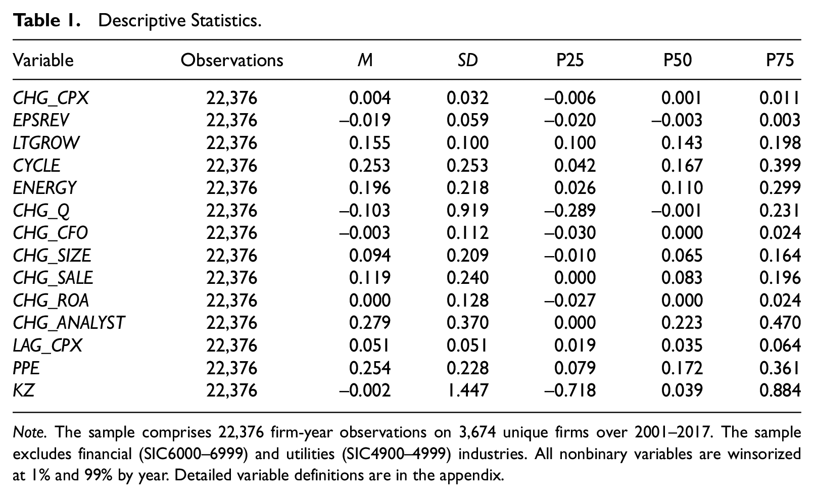
Note. The sample comprises 22,376 firm-year observations on 3,674 unique firms over 2001–2017. The sample excludes financial (SIC6000–6999) and utilities (SIC4900–4999) industries. All nonbinary variables are winsorized at 1% and 99% by year. Detailed variable definitions are in the appendix.

Our proxies for analyst information advantage, CYCLE and ENERGY, have a mean of 0.253 and 0.196, respectively, and medians of 0.167 and 0.110, respectively, suggesting that our sample firms have nontrivial exposures to macroeconomic factors in general.¹⁴ There is also substantial cross-sectional variation in the exposure, as evidenced by standard deviations of 0.253 for CYCLE and 0.218 for ENERGY.

As to the control variables, change in Tobin’s Q (CHG_Q) has a small negative mean and median of −0.103 and −0.001, respectively. Change in cash flow (CHG_CFO) and change in return on assets (CHG_ROA) both have means and medians close to zero. On average, firm size increases annually by about 9.4% (CHG_SIZE), whereas sales has an annual increase rate of about 11.9% (CHG_SALE). Analyst coverage also has a small positive average increase of 0.279 (CHG_ANALYST). Firms’ annual capital expenditure is about 5.1% of total assets (LAG_CPX), consistent with prior research with similar data requirements (e.g., Ramalingegowda et al., 2013).

Empirical Results

Investment-Forecast Sensitivity

Before examining the managerial learning hypothesis, we focus on the relationship between managers’ investment decisions and analyst information by estimating Model (2). In Table 2, we include our measures of analyst information, EPSREV and LTGROW, in Columns (1) and (2), respectively, and then include both measures in one regression in Column (3).

Table 2.

Investment-Forecast Sensitivity: Relation Between Change in Capital Expenditure and Analyst Forecast.

Dependent variable = CHG_CPX	(1)	(2)	(3)
EPSREV	0.0895***		0.0863***
	(0.0079)		(0.0078)
LTGROW		0.0288***	0.0242***
		(0.0042)	(0.0041)
CHG_Q	0.0028***	0.0037***	0.0028***
	(0.0003)	(0.0003)	(0.0003)
CHG_CFO	0.0076	0.0161**	0.0090
	(0.0082)	(0.0082)	(0.0081)
CHG_SIZE	0.0037**	0.0073***	0.0035**
	(0.0016)	(0.0016)	(0.0016)
CHG_SALE	0.0067***	0.0067***	0.0053***
	(0.0016)	(0.0017)	(0.0016)
CHG_ROA	−0.0037	−0.0045	−0.0059
	(0.0075)	(0.0077)	(0.0074)
CHG_ANALYST	0.0016**	0.0022***	0.0015*
	(0.0008)	(0.0008)	(0.0008)
LAG_CPX	−0.4757***	−0.4865***	−0.4774***
	(0.0225)	(0.0225)	(0.0224)
CONSTANT	0.0284***	0.0199***	0.0237***
	(0.0018)	(0.0020)	(0.0020)
Firm-fixed effects	Yes	Yes	Yes
Year-fixed effects	Yes	Yes	Yes
Observations	22,376	22,376	22,376
Adjusted R²	.255	.243	.258

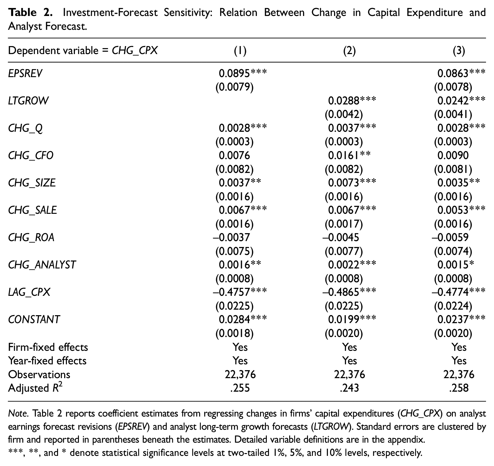
Note. Table 2 reports coefficient estimates from regressing changes in firms’ capital expenditures (CHG_CPX) on analyst earnings forecast revisions (EPSREV) and analyst long-term growth forecasts (LTGROW). Standard errors are clustered by firm and reported in parentheses beneath the estimates. Detailed variable definitions are in the appendix.

***

, **, and * denote statistical significance levels at two-tailed 1%, 5%, and 10% levels, respectively.

As expected, we find that changes in capital investment are positively associated with both of our measures of analyst information, suggesting that analyst forecasts contain investment-relevant information. In Column (1), the coefficient on EPSREV is 0.0895 and statistically significant at the .01 level. Similarly, in Column (2), the coefficient on LTGROW is 0.0288 and statistically significant at the .01 level. In Column (3), when we include both measures of analyst information in one regression as specified in Model (2), the coefficients remain statistically significant, with magnitudes only slightly lower than those reported in Columns (1) and (2), where the analyst variable is individually included. This suggests that EPSREV and LTGROW may capture different aspects of analysts’ forecasts of firm prospects and have limited overlapping information.

We discuss the economic significance of the coefficients in Column (3). The coefficient on EPSREV is 0.0863, suggesting that a 1-standard-deviation increase in analyst earnings forecast revision is associated with an increase in investment change of 0.0051 [0.0863 × 0.059], equivalent to 16% [0.0863 × 0.059 / 0.032] of the sample standard deviation of investment change. Similarly, the coefficient on LTGROW is 0.0242, which suggests that a 1-standard-deviation increase in analyst long-term growth forecasts is associated with an increase of about 7% [0.0242 × 0.100 / 0.032] of the sample standard deviation of investment change.

As to the control variables, we find that changes in investment are significantly and positively associated with changes in Tobin’s Q (CHG_Q). This is consistent with Tobin’s Q theory and the literature on investment-price sensitivity (e.g., Chen et al., 2007; Erickson & Whited, 2000). Importantly, the investment-forecast sensitivity is significantly positive even after we control for investment-price sensitivity. While in an efficient market, analyst information is expected to be reflected in stock prices, the incremental effects of analyst information in the presence of stock prices suggest that analyst forecasts may contain information that has unique and different implications for corporate investments than other information contained in stock prices. The effects of other control variables are largely consistent with the literature. Changes in firm size (CHG_SIZE), sales growth (CHG_SALE), and analyst coverage (CHG_ANALYST) are significantly and positively associated with changes in investment. Firms that have higher prior capital expenditures (LAG_CPX) tend to have lower changes in investment.

Overall, Table 2 suggests that managers’ investment decisions are positively associated with the information in analyst forecasts of earnings performance and long-term growth. However, as discussed above, such an association could be due to both the correlated information between the two parties and the managerial learning from analysts, and therefore does not directly shed light on the learning hypothesis. We next test the learning hypothesis.

Managerial Learning From Analysts

To test the managerial learning hypothesis, we examine whether the sensitivity of investment to analyst information increases with CYCLE and ENERGY, our proxies for analyst information advantage. A higher value of CYCLE or ENERGY indicates analysts’ information advantage over managers with respect to the implications of macroeconomic factors (the business cycle and energy prices, respectively) for the firm operations.

Table 3 presents the empirical results of testing the managerial learning hypothesis based on Model (3). Columns (1) to (3) test for managerial learning with respect to analyst information advantage related to the business cycle (CYCLE), and Columns (4) to (6) test for that related to energy prices (ENERGY). In all columns, the coefficients on EPSREV and LTGROW remain significantly positive as documented in Table 2.

Table 3.

Managerial Learning: Relation Between Investment-Forecast Sensitivity and Analyst Information Advantage.

Dependent variable = CHG_CPX	(1)	(2)	(3)	(4)	(5)	(6)
EPSREV	0.0691***		0.0686***	0.0642***		0.0635***
	(0.0097)		(0.0096)	(0.0086)		(0.0086)
LTGROW		0.0184***	0.0129***		0.0189***	0.0153***
		(0.0049)	(0.0048)		(0.0046)	(0.0045)
CYCLE	0.0076***	−0.0001	0.0006
	(0.0012)	(0.0023)	(0.0023)
EPSREV×CYCLE	0.1039***		0.0943***
	(0.0325)		(0.0316)
LTGROW×CYCLE		0.0381***	0.0404***
		(0.0139)	(0.0136)
ENERGY				0.0060***	−0.0036	−0.0005
				(0.0015)	(0.0030)	(0.0030)
EPSREV×ENERGY				0.1507***		0.1366***
				(0.0401)		(0.0387)
LTGROW×ENERGY					0.0456***	0.0381**
					(0.0176)	(0.0172)
CHG_Q	0.0027***	0.0036***	0.0027***	0.0027***	0.0037***	0.0027***
	(0.0003)	(0.0003)	(0.0003)	(0.0003)	(0.0003)	(0.0003)
CHG_CFO	0.0082	0.0162**	0.0095	0.0083	0.0161**	0.0095
	(0.0079)	(0.0079)	(0.0076)	(0.0081)	(0.0082)	(0.0080)
CHG_SIZE	0.0030*	0.0068***	0.0027*	0.0036**	0.0070***	0.0033**
	(0.0016)	(0.0016)	(0.0016)	(0.0016)	(0.0016)	(0.0016)
CHG_SALE	0.0055***	0.0058***	0.0039**	0.0061***	0.0063***	0.0047***
	(0.0016)	(0.0017)	(0.0016)	(0.0016)	(0.0017)	(0.0016)
CHG_ROA	−0.0047	−0.0054	−0.0073	−0.0045	−0.0051	−0.0068
	(0.0072)	(0.0073)	(0.0069)	(0.0074)	(0.0076)	(0.0073)
CHG_ANALYST	0.0016**	0.0021***	0.0015*	0.0016**	0.0022***	0.0015**
	(0.0008)	(0.0008)	(0.0008)	(0.0008)	(0.0008)	(0.0008)
LAG_CPX	−0.4785***	−0.4885***	−0.4803***	−0.4770***	−0.4872***	−0.4787***
	(0.0226)	(0.0225)	(0.0225)	(0.0224)	(0.0224)	(0.0223)
CONSTANT	0.0269***	0.0202***	0.0241***	0.0275***	0.0208***	0.0243***
	(0.0019)	(0.0020)	(0.0020)	(0.0019)	(0.0019)	(0.0019)
Firm-fixed effects	Yes	Yes	Yes	Yes	Yes	Yes
Year-fixed effects	Yes	Yes	Yes	Yes	Yes	Yes
Observations	22,376	22,376	22,376	22,376	22,376	22,376
Adjusted R²	.258	.245	.262	.258	.244	.262

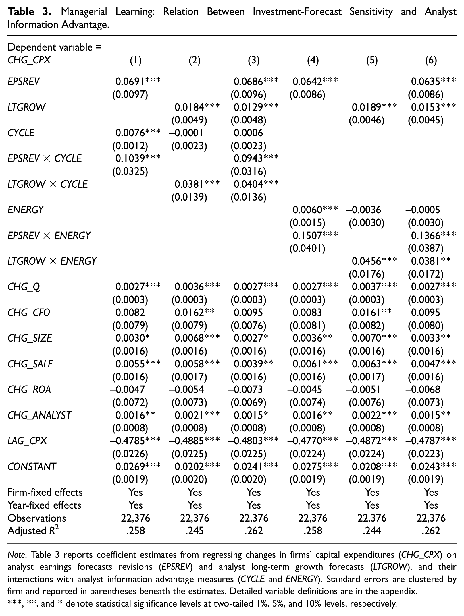
Note. Table 3 reports coefficient estimates from regressing changes in firms’ capital expenditures (CHG_CPX) on analyst earnings forecasts revisions (EPSREV) and analyst long-term growth forecasts (LTGROW), and their interactions with analyst information advantage measures (CYCLE and ENERGY). Standard errors are clustered by firm and reported in parentheses beneath the estimates. Detailed variable definitions are in the appendix.

***

, **, and * denote statistical significance levels at two-tailed 1%, 5%, and 10% levels, respectively.

Our main interest, however, is in the interaction terms between the analyst forecast variables and our proxies for analyst information advantage. For each proxy for analyst information advantage, we first estimate reduced versions of Model (3) by interacting it with only one analyst forecast variable (Columns (1) and (2) for CYCLE and Columns (4) and (5) for ENERGY), and then estimate the full version of Model (3) (Column (3) for CYCLE and Column (6) for ENERGY). In general, we find similar implications of the interaction terms for the reduced and the full versions. We therefore focus on discussing the results in Columns (3) and (6). As Column (3) shows, the coefficient on EPSREV×CYCLE is 0.0943 and is significant at the .01 level, suggesting that the investment-forecast sensitivity based on analyst earnings forecast revisions is higher for firms with greater exposures to the macroeconomic business cycle and hence a higher analyst information advantage. A 1-standard-deviation increase in CYCLE increases the investment-EPSREV sensitivity by 0.0238 [0.253 × 0.0943], representing a 28% increase relative to the sensitivity of 0.0843 [0.0686 + 0.0943 × 0.167] for a firm with the sample median CYCLE. The coefficient on LTGROW×CYCLE is also significant at the .01 level, with a magnitude of 0.0404. As CYCLE increases by 1 standard deviation, the investment-LTGROW sensitivity increases by 0.0102 [0.253 × 0.0404], representing a 52% increase relative to the sensitivity of 0.0196 [0.0129 + 0.0404 × 0.167] for a firm with sample median CYCLE.

In Column (6), the results are consistent with managerial learning on energy price-related information from analyst forecasts. The coefficient on EPSREV × ENERGY is 0.1366 and significant at the .01 level. A 1-standard-deviation increase in ENERGY increases investment-ESPREV sensitivity by 0.0298 [0.218×0.1366], 38% higher than the sensitivity of 0.0785 [0.0635 + 0.110 × 0.1366] for a firm with sample median ENERGY. The coefficient on LTGROW × ENERGY is 0.0381 and significant at the .05 level. A 1-standard-deviation increase in ENERGY increases investment-LTGROW sensitivity by 0.0083 [0.218 × 0.0381], representing a 43% increase relative to the sensitivity of 0.0195 [0.0153 + 0.110 × 0.0381] for a firm with sample median ENERGY.¹⁵

Overall, the results in Table 3 show that analyst information advantage, as captured by CYCLE and ENERGY, affects the relation between corporate investments and analyst forecast information, supporting the learning hypothesis that managers learn from financial analysts in making investment decisions.¹⁶

Analyst Information Advantage

The premise of our research is that analysts have an information advantage over managers in predicting the implications of macroeconomic factors for firm performance and prospects (Hutton et al., 2012). If this is indeed the case, we should expect our results to concentrate among firms whose analysts have greater expertise or insights related to macroeconomic factors. We test this expectation using two proxies for a firm’s analyst macroeconomic advantage: (a) whether the analysts cover more industries and (b) whether the analysts are from a larger broker which is more likely to host in-house macroeconomists.

To construct our first proxy, we obtain the number of industries (based on two-digit SIC codes) covered by each analyst following a firm and then calculate the maximum number of the industries covered by the analysts for each firm-year. We divide our sample based on the median value of the proxy, then estimate Model (3) in each of the two subsamples. For our second proxy, we identify a broker as a larger broker if it is among the top 10 brokers based on the number of analysts contributing to I/B/E/S in the year. We divide our sample based on whether at least one of a firm’s analysts is from a larger broker and estimate Model (3) in each of the two subsamples.

The results based on the two proxies are reported in Table 4, Panels A and B, respectively. In both panels, we find that the coefficients of the four interaction terms, EPSREV×CYCLE and LTGROW×CYCLE (or ×ENERGY), are statistically significant only in firms with analysts who are more likely to have macroeconomic information advantage (i.e., who cover more industries or who are employed by larger brokers).¹⁷ The coefficients are insignificant (except EPSREV×ENERGY in Panel A) when analysts cover fewer industries or when they work for smaller brokers that are less likely to host in-house economists. Overall, these results suggest that our main results are indeed driven by analysts’ specific insights and knowledge about the macroeconomy, lending further support to our hypothesis that managers learn from analysts about the implications of macroeconomic information for their individual firms.

Table 4.

Managerial Learning: Analyst Information Advantage on Macroeconomic Factors.

Panel A: Industry covered	(1)	(2)	(3)	(4)
Dependent variable = CHG_CPX	Less advantage	More advantage	Less advantage	More advantage
EPSREV	0.0622***	0.0638***	0.0564***	0.0563***
	(0.0144)	(0.0140)	(0.0130)	(0.0122)
LTGROW	0.0102	0.0166**	0.0163**	0.0184***
	(0.0079)	(0.0068)	(0.0077)	(0.0065)
CYCLE	0.0003	−0.0006
	(0.0041)	(0.0034)
EPSREV×CYCLE	0.0731	0.1063**
	(0.0509)	(0.0450)
LTGROW×CYCLE	0.0309	0.0470**
	(0.0205)	(0.0206)
ENERGY			0.0045	−0.0017
			(0.0052)	(0.0039)
EPSREV×ENERGY			0.1080*	0.1746***
			(0.0599)	(0.0472)
LTGROW×ENERGY			0.0095	0.0442*
			(0.0264)	(0.0233)
CHG_Q	0.0023***	0.0030***	0.0023***	0.0031***
	(0.0005)	(0.0005)	(0.0005)	(0.0005)
CHG_CFO	−0.0177	0.0222*	−0.0180	0.0227*
	(0.0192)	(0.0116)	(0.0194)	(0.0122)
CHG_SIZE	0.0007	0.0023	0.0012	0.0029
	(0.0027)	(0.0021)	(0.0027)	(0.0021)
CHG_SALE	0.0041	0.0041*	0.0047	0.0047**
	(0.0029)	(0.0023)	(0.0028)	(0.0024)
CHG_ROA	0.0173	−0.0178	0.0181	−0.0180
	(0.0181)	(0.0109)	(0.0183)	(0.0115)
CHG_ANALYST	0.0027*	0.0006	0.0027*	0.0006
	(0.0014)	(0.0010)	(0.0014)	(0.0010)
LAG_CPX	−0.5857***	−0.4423***	−0.5864***	−0.4394***
	(0.0340)	(0.0321)	(0.0340)	(0.0320)
CONSTANT	0.0297***	0.0223***	0.0290***	0.0226***
	(0.0038)	(0.0027)	(0.0038)	(0.0027)
Firm-fixed effects	Yes	Yes	Yes	Yes
Year-fixed effects	Yes	Yes	Yes	Yes
Observations	8,578	13,798	8,578	13,798
Adjusted R²	.300	.300	.300	.300
Panel B: Brokerage size	(1)	(2)	(3)	(4)
Dependent variable = CHG_CPX	Less advantage	More advantage	Less advantage	More advantage
EPSREV	0.0742***	0.0690***	0.0861***	0.0605***
	(0.0189)	(0.0119)	(0.0182)	(0.0104)
LTGROW	0.0155	0.0127**	0.0177	0.0142***
	(0.0168)	(0.0050)	(0.0168)	(0.0047)
CYCLE	0.0083	0.0004
	(0.0070)	(0.0026)
EPSREV×CYCLE	0.0922	0.1009***
	(0.0663)	(0.0391)
LTGROW×CYCLE	0.0041	0.0407***
	(0.0357)	(0.0153)
ENERGY			0.0047	−0.0002
			(0.0082)	(0.0033)
EPSREV×ENERGY			0.0227	0.1668***
			(0.0640)	(0.0490)
LTGROW×ENERGY			0.0023	0.0410**
			(0.0429)	(0.0193)
CHG_Q	0.0017*	0.0027***	0.0019**	0.0028***
	(0.0009)	(0.0004)	(0.0009)	(0.0004)
CHG_CFO	−0.0244	0.0142*	−0.0269	0.0145*
	(0.0402)	(0.0077)	(0.0427)	(0.0080)
CHG_SIZE	0.0029	0.0020	0.0040	0.0025
	(0.0045)	(0.0018)	(0.0045)	(0.0017)
CHG_SALE	0.0024	0.0042**	0.0035	0.0048**
	(0.0039)	(0.0019)	(0.0039)	(0.0019)
CHG_ROA	0.0159	−0.0093	0.0184	−0.0092
	(0.0396)	(0.0069)	(0.0423)	(0.0071)
CHG_ANALYST	0.0008	0.0015*	0.0008	0.0016*
	(0.0019)	(0.0009)	(0.0020)	(0.0009)
LAG_CPX	−0.6103***	−0.4629***	−0.6080***	−0.4611***
	(0.0466)	(0.0242)	(0.0464)	(0.0240)
CONSTANT	0.0317***	0.0233***	0.0318***	0.0235***
	(0.0056)	(0.0021)	(0.0056)	(0.0021)
Firm-fixed effects	Yes	Yes	Yes	Yes
Year-fixed effects	Yes	Yes	Yes	Yes
Observations	4,140	18,236	4,140	18,236
Adjusted R²	.311	.265	.309	.266

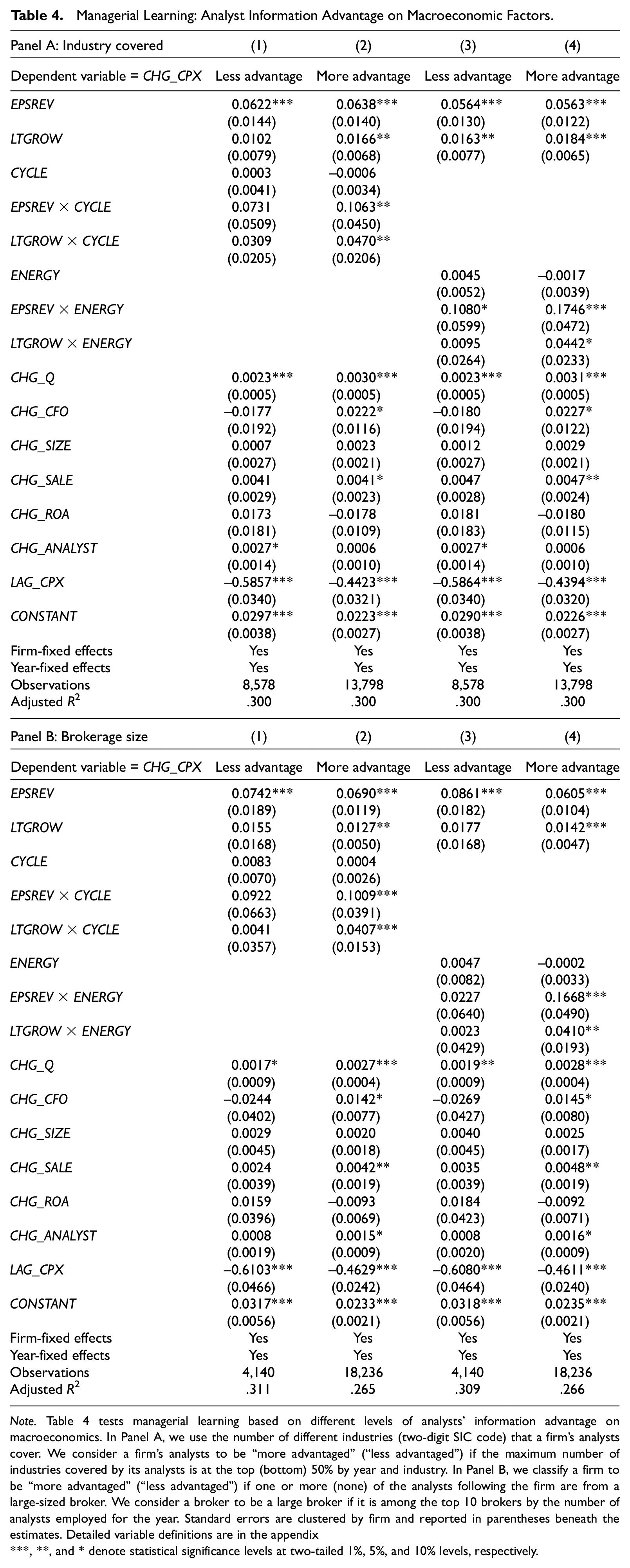
Note. Table 4 tests managerial learning based on different levels of analysts’ information advantage on macroeconomics. In Panel A, we use the number of different industries (two-digit SIC code) that a firm’s analysts cover. We consider a firm’s analysts to be “more advantaged” (“less advantaged”) if the maximum number of industries covered by its analysts is at the top (bottom) 50% by year and industry. In Panel B, we classify a firm to be “more advantaged” (“less advantaged”) if one or more (none) of the analysts following the firm are from a large-sized broker. We consider a broker to be a large broker if it is among the top 10 brokers by the number of analysts employed for the year. Standard errors are clustered by firm and reported in parentheses beneath the estimates. Detailed variable definitions are in the appendix

***

, **, and * denote statistical significance levels at two-tailed 1%, 5%, and 10% levels, respectively.

Effects of Firm Capital Intensity

Managers’ incentives to learn from analysts are likely to increase with the importance of capital investments to their firms. Accordingly, we use a firm’s capital intensity as a proxy for managers’ learning incentives and examine whether managerial learning concentrates among firms with higher capital intensity. We measure capital intensity as the percentage of net plant, property, and equipment (PPE) relative to total assets. We divide our sample into subsamples with high and low PPE intensity based on the sample medians of capital intensity by year and industry. Table 5 reports the results.

Table 5.

Managerial Learning: Firms’ Capital Intensity.

Dependent variable = CHG_CPX	(1)	(2)	(3)	(4)
Dependent variable = CHG_CPX	Low intensity	High intensity	Low intensity	High intensity
EPSREV	0.0134**	0.0901***	0.0170***	0.0904***
	(0.0062)	(0.0157)	(0.0056)	(0.0140)
LTGROW	0.0036	0.0118	0.0083	0.0147**
	(0.0048)	(0.0072)	(0.0051)	(0.0067)
CYCLE	0.0005	0.0021
	(0.0020)	(0.0039)
EPSREV×CYCLE	0.0419	0.1428***
	(0.0275)	(0.0452)
LTGROW×CYCLE	0.0188	0.0625***
	(0.0115)	(0.0241)
ENERGY			0.0014	0.0013
			(0.0024)	(0.0045)
EPSREV×ENERGY			0.0291	0.1482**
			(0.0257)	(0.0647)
LTGROW×ENERGY			0.0037	0.0575**
			(0.0148)	(0.0265)
CHG_Q	0.0016***	0.0061***	0.0016***	0.0063***
	(0.0003)	(0.0009)	(0.0003)	(0.0009)
CHG_CFO	0.0070**	−0.0033	0.0071*	−0.0057
	(0.0036)	(0.0393)	(0.0037)	(0.0419)
CHG_SIZE	0.0032**	0.0063*	0.0035***	0.0072**
	(0.0013)	(0.0037)	(0.0013)	(0.0036)
CHG_SALE	0.0014	0.0052	0.0020	0.0060*
	(0.0014)	(0.0032)	(0.0014)	(0.0032)
CHG_ROA	−0.0053	0.0146	−0.0049	0.0172
	(0.0033)	(0.0403)	(0.0034)	(0.0429)
CHG_ANALYST	0.0015**	0.0024*	0.0015**	0.0024*
	(0.0007)	(0.0015)	(0.0007)	(0.0015)
LAG_CPX	−0.5598***	−0.4683***	−0.5584***	−0.4646***
	(0.0652)	(0.0226)	(0.0654)	(0.0225)
CONSTANT	0.0135***	0.0356***	0.0131***	0.0355***
	(0.0025)	(0.0030)	(0.0026)	(0.0030)
Firm-fixed effects	Yes	Yes	Yes	Yes
Year-fixed effects	Yes	Yes	Yes	Yes
Observations	11,182	11,194	11,182	11,194
Adjusted R²	.325	.297	.323	.296

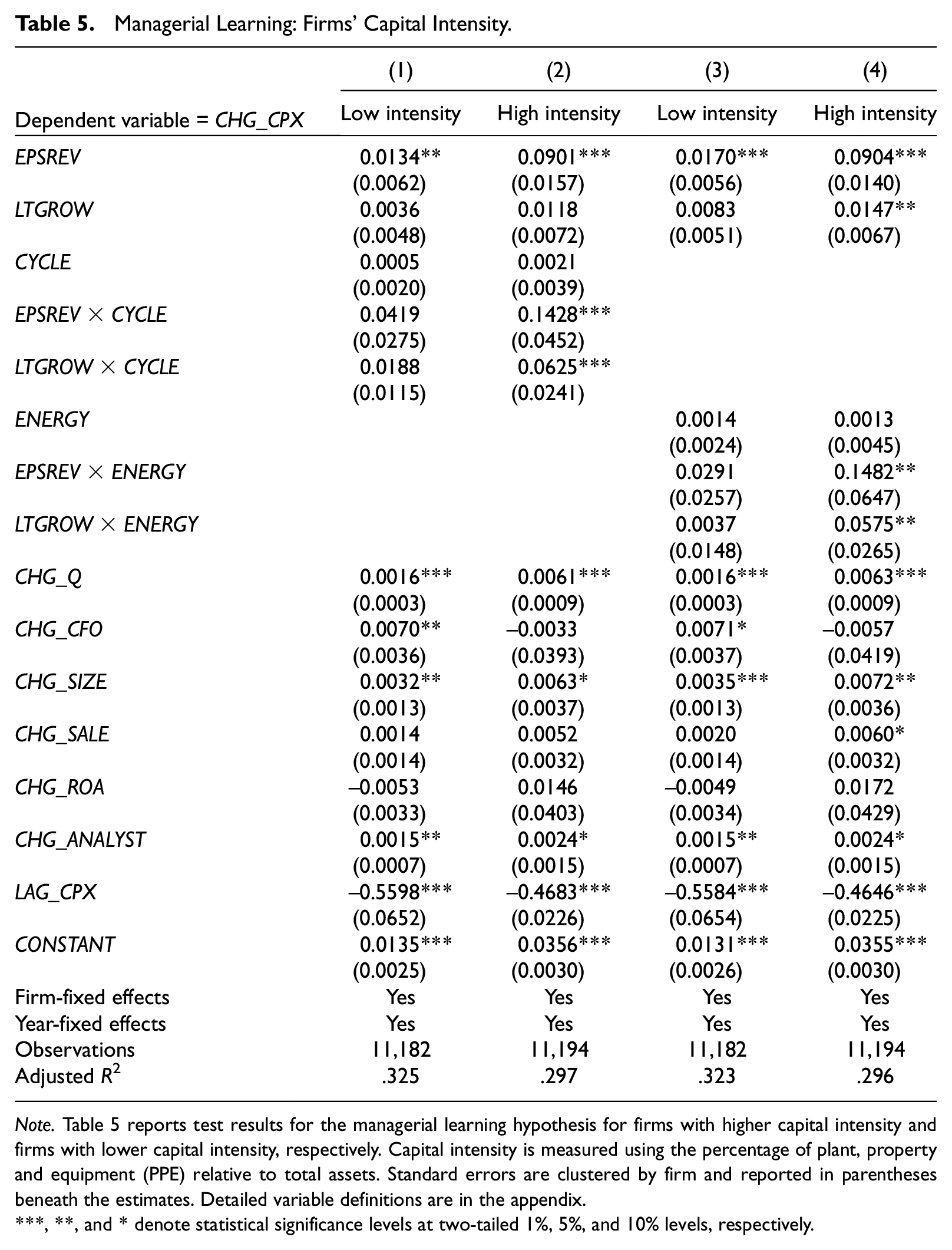
Note. Table 5 reports test results for the managerial learning hypothesis for firms with higher capital intensity and firms with lower capital intensity, respectively. Capital intensity is measured using the percentage of plant, property and equipment (PPE) relative to total assets. Standard errors are clustered by firm and reported in parentheses beneath the estimates. Detailed variable definitions are in the appendix.

***

, **, and * denote statistical significance levels at two-tailed 1%, 5%, and 10% levels, respectively.

We find that for firms with high capital intensity, the coefficients on the interaction terms between analyst forecasts variables and our proxies for analyst information advantage are statistically significant, which suggests that managers of firms with high capital intensity learn from analyst earnings forecasts and long-term growth forecasts with respect to the implications of the business cycle or energy prices. However, for firms with low capital intensity, the coefficients on the interaction terms are not statistically insignificant, suggesting little managerial learning.

Overall, we show that the effects of firm exposures to macroeconomic factors on investment-forecast sensitivity are primarily attributable to firms with higher capital intensity. To the extent that firms with higher capital intensity have greater incentives to learn from analysts, these results suggest that our main results in Table 3 are attributable to learning, providing further support for the hypothesis that managers learn from analysts with respect to the implications of macroeconomic factors for firm prospects.

Alternative Explanations and Tests

We emphasize that our inferences on managerial learning are not based on the investment-forecast sensitivity itself but are based on how this sensitivity varies with proxies for analyst information advantage relative to managers on the firm-specific implications of macroeconomic factors. Thus, any potential alternative explanations need to explain this cross-sectional effect on the investment-forecast sensitivity.

For example, one may argue that analysts cater to managers by issuing forecasts consistent with managers’ investment decisions, which leads to higher investment-forecast sensitivity. For this explanation to impose a credible threat to our hypothesis, it needs to explain why catering is stronger when firms have greater exposure to macroeconomic factors. However, this is unlikely because one would expect analysts to have stronger incentives to cater to managers when managers are better informed than analysts (Ke & Yu, 2006), not when analysts are better informed than managers (i.e., when the firms have higher exposures to macroeconomic factors). We next address several potential alternative explanations that are possibly correlated with a firm’s exposures to macroeconomic factors.

Investment Sensitivity to Macroeconomic Factors

One potential alternative explanation for our results is that for firms with greater exposure to macro factors, their investments are likely to have greater sensitivity to those factors too. In other words, managers of these firms are more likely to pay attention to macroeconomic information and invest accordingly. At the same time, analysts are well-informed at the macroeconomic level, and their forecasts also contain more information about macroeconomic factors for these firms. Thus, our results could be either mechanical or attributable to managers learning about macroeconomic information in general, not specifically from analysts.

However, analysts do not issue forecasts on macroeconomic factors. Their forecasts are firm-specific. In other words, analysts capitalize on their access to macroeconomic information and their insights and expertise on the operations of the economy, the industry, and the firm and analyze firm-specific implications of the macro-level data accordingly. They incorporate these firm-specific implications into their earnings forecasts and long-term growth forecasts for a given firm.

Managers, on the contrary, have less access to macroeconomic information and are also substantially less skilled in analyzing how such information affects their own firm’s prospects (Anilowski et al., 2007; Hutton et al., 2012; Kim et al., 2016). Thus, what managers desire to learn from analysts is not about macroeconomic factors, but about the implications of such factors for their own firms’ specific prospects. This type of firm-specific information is generally not available from sources other than analysts.

To support this point, we directly control for macroeconomic factors and their interactions with firm exposure to macroeconomic factors (i.e., our proxy for analyst information advantage). If our results are completely driven by the greater sensitivity of firm investments to macroeconomic factors for firms with higher exposures to these factors, rather than by analysts’ firm-specific information related to these factors, our results should become insignificant once we explicitly control for macroeconomic factors.

We seek to control for forecasts of macroeconomic factors available at the end of the year t. For GDP growth, we use the Survey of Professional Forecasters administered by the Federal Reserve Bank of Philadelphia.¹⁸ We were not able to find forecast data for energy prices for our sample period; therefore, we control for realized future price changes available from the International Monetary Fund.¹⁹

We report the results in Table 6. Columns (1) to (3) control for GDPFCST, the average GDP growth forecasts for the next four quarters, and its interaction with analyst information advantage proxy CYCLE. Consistent with the results in Table 3, the coefficients of EPSREV×CYCLE and LTGROW×CYCLE remain positive and statistically significant at the .01 levels. In Columns (4) to (6), we control for FWD_EINDEX, the change in energy index from year t to year t+ 1, and its interaction with analyst information advantage proxy ENERGY. The coefficients of EPSREV×ENERGY and LTGROW×ENERGY remain positive and statistically significant at the .01 and .05 levels, respectively. The magnitudes of the coefficients on the interaction terms remain comparable with the corresponding coefficients in Table 3.

Table 6.

Managerial Learning: Control for Macroeconomic Factors.

Dependent variable = CHG_CPX	(1)	(2)	(3)	(4)	(5)	(6)
EPSREV	0.0715***		0.0706***	0.0669***		0.0662***
	(0.0097)		(0.0097)	(0.0087)		(0.0087)
LTGROW		0.0184***	0.0128***		0.0193***	0.0155***
		(0.0048)	(0.0047)		(0.0046)	(0.0045)
CYCLE	0.0114***	0.0068	0.0058
	(0.0043)	(0.0048)	(0.0048)
EPSREV×CYCLE	0.1035***		0.0951***
	(0.0324)		(0.0316)
LTGROW×CYCLE		0.0387***	0.0408***
		(0.0139)	(0.0136)
ENERGY				0.0055***	−0.0038	−0.0008
				(0.0015)	(0.0030)	(0.0030)
EPSREV×ENERGY				0.1494***		0.1356***
				(0.0401)		(0.0387)
LTGROW×ENERGY					0.0442**	0.0368**
					(0.0175)	(0.0171)
GDPFCST	0.0491**	0.0102	0.0274
	(0.0238)	(0.0244)	(0.0239)
GDPFCST×CYCLE	−0.0014	−0.0026	−0.0019
	(0.0016)	(0.0016)	(0.0016)
FWD_EINDEX				0.1949**	0.0485	0.1175
				(0.0902)	(0.0925)	(0.0905)
FWD_EINDEX×ENERGY				0.0326	0.0296	0.0286
				(0.0271)	(0.0276)	(0.0270)
CHG_Q	0.0028***	0.0038***	0.0028***	0.0028***	0.0039***	0.0029***
	(0.0003)	(0.0003)	(0.0003)	(0.0003)	(0.0003)	(0.0003)
CHG_CFO	0.0074	0.0156**	0.0087	0.0076	0.0157*	0.0088
	(0.0079)	(0.0079)	(0.0076)	(0.0081)	(0.0082)	(0.0079)
CHG_SIZE	0.0032**	0.0071***	0.0029*	0.0038**	0.0074***	0.0035**
	(0.0016)	(0.0016)	(0.0016)	(0.0016)	(0.0016)	(0.0016)
CHG_SALE	0.0055***	0.0060***	0.0040**	0.0062***	0.0066***	0.0047***
	(0.0016)	(0.0017)	(0.0016)	(0.0016)	(0.0017)	(0.0016)
CHG_ROA	−0.0041	−0.0047	−0.0067	−0.0040	−0.0045	−0.0063
	(0.0072)	(0.0073)	(0.0069)	(0.0074)	(0.0076)	(0.0072)
CHG_ANALYST	0.0018**	0.0024***	0.0017**	0.0018**	0.0024***	0.0017**
	(0.0008)	(0.0008)	(0.0008)	(0.0008)	(0.0008)	(0.0008)
LAG_CPX	−0.4796***	−0.4902***	−0.4815***	−0.4782***	−0.4894***	−0.4801***
	(0.0224)	(0.0223)	(0.0224)	(0.0223)	(0.0223)	(0.0222)
CONSTANT	−0.0970*	−0.0070	−0.0457	0.0216***	0.0182***	0.0202***
	(0.0583)	(0.0598)	(0.0586)	(0.0019)	(0.0020)	(0.0020)
Firm-fixed effects	Yes	Yes	Yes	Yes	Yes	Yes
Year-fixed effects	Yes	Yes	Yes	Yes	Yes	Yes
Observations	22,376	22,376	22,376	22,376	22,376	22,376
Adjusted R²	.257	.244	.261	.257	.242	.260

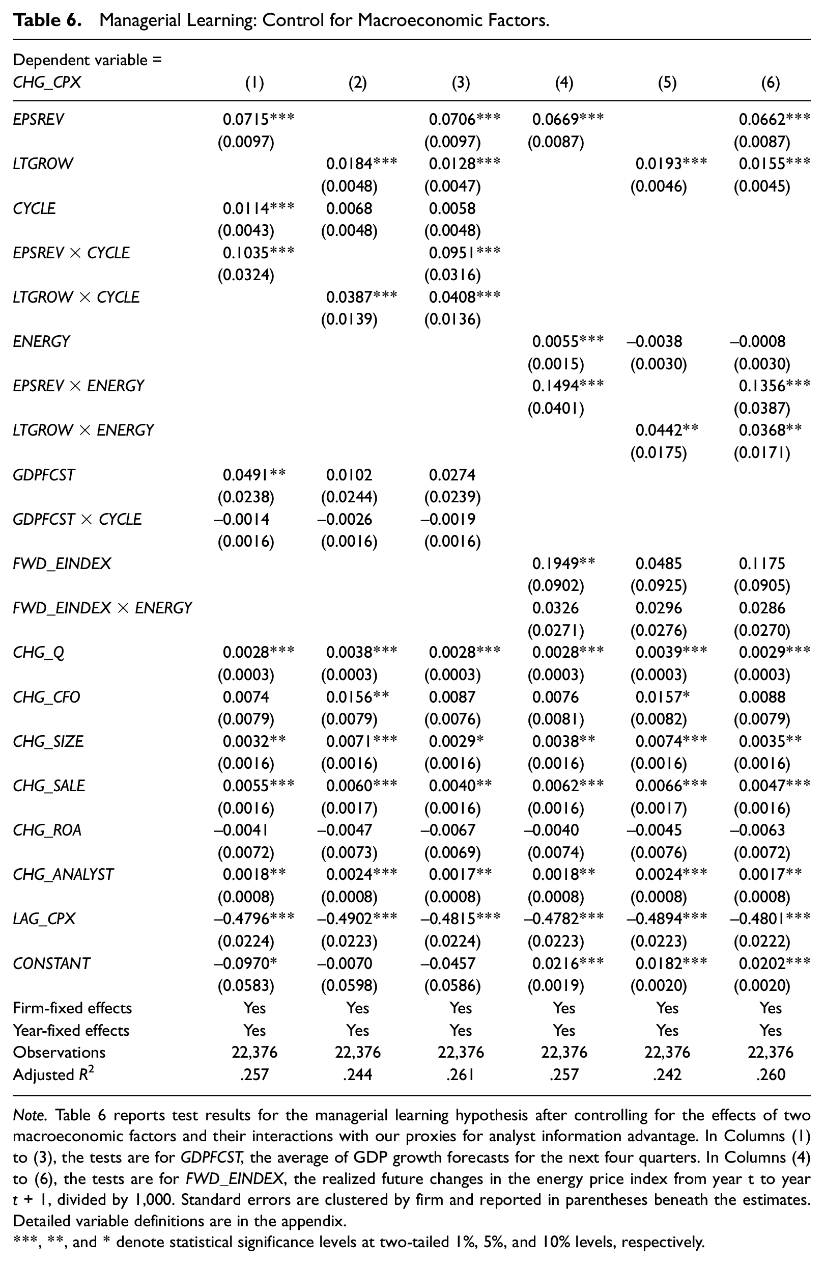
Note. Table 6 reports test results for the managerial learning hypothesis after controlling for the effects of two macroeconomic factors and their interactions with our proxies for analyst information advantage. In Columns (1) to (3), the tests are for GDPFCST, the average of GDP growth forecasts for the next four quarters. In Columns (4) to (6), the tests are for FWD_EINDEX, the realized future changes in the energy price index from year t to year t+ 1, divided by 1,000. Standard errors are clustered by firm and reported in parentheses beneath the estimates. Detailed variable definitions are in the appendix.

***

, **, and * denote statistical significance levels at two-tailed 1%, 5%, and 10% levels, respectively.

As to the macroeconomic factors, GDPFCST is significantly positive in Column (1). However, the interaction terms of GDPFCST and CYCLE in Columns (1) to (3) are insignificant. Similarly, in Columns (4) to (6), the interaction terms of FWD_EINDEX and ENERGY are insignificant. These results suggest that the sensitivity of firm investments to macroeconomic factors does not vary with the exposure of firm operations to these macroeconomic factors. We check the robustness of these results after dropping the interaction terms EPSREV×CYCLE and LTGROW×CYCLE or further removing the analyst forecasts variables EPSREV and LTGROW. The inferences related to learning from GDPFCST or FWD_EINDEX remain the same.

Overall, the results in Table 6 confirm our conjecture that our results are not driven by managers learning about macroeconomic factors, but rather by managers learning from analysts about the firm-specific implications of the macroeconomic factors contained in analyst forecasts.

Bellwether Firms

Prior literature suggests that bellwether firms convey more news about the macroeconomy, and their earnings are informative about the economy (e.g., Anilowski et al., 2007; Barth & So, 2014). Given the way that we measure a firm’s exposure to macroeconomic factors, bellwether firms are likely identified as those with more exposure. For these firms, even if managers’ investment decisions reflect firm-specific information, they can be indicative of macroeconomic information. Such information can have a high correlation with analyst forecasts to the extent that analyst forecasts also contain a greater amount of macroeconomic information for these firms. This provides a potential alternative explanation for our results in Table 3.

To rule out this alternative explanation, we re-estimate Model (3) by excluding bellwether firms, proxied by S&P 500 member firms and by larger firms (e.g., Anilowski et al., 2007; Barth & So, 2014; Hann et al., 2019). Specifically, we remove S&P 500 firms and label the remaining observations as Non-S&P 500 Firms. Alternatively, we remove observations in the top 20% of firm size by year and industry in our sample and label the remaining observations as Small Firms. Table 7 reports the results for these two subsamples separately.

Table 7.

Managerial Learning: Non-S&P 500 Firms and Small Firms.

	(1)	(2)	(3)	(4)
Dependent variable = CHG_CPX	Non-S&P 500 firms		Small firms
EPSREV	0.0651***	0.0635***	0.0631***	0.0582***
	(0.0104)	(0.0096)	(0.0105)	(0.0096)
LTGROW	0.0128**	0.0153***	0.0155***	0.0171***
	(0.0056)	(0.0054)	(0.0054)	(0.0052)
CYCLE	0.0017		0.0023
	(0.0030)		(0.0029)
EPSREV×CYCLE	0.0868**		0.0937***
	(0.0347)		(0.0355)
LTGROW×CYCLE	0.0361**		0.0357**
	(0.0163)		(0.0159)
ENERGY		−0.0000		−0.0003
		(0.0039)		(0.0037)
EPSREV×ENERGY		0.1065***		0.1307***
		(0.0408)		(0.0420)
LTGROW×ENERGY		0.0341*		0.0388*
		(0.0206)		(0.0204)
CHG_Q	0.0028***	0.0029***	0.0028***	0.0029***
	(0.0004)	(0.0004)	(0.0004)	(0.0004)
CHG_CFO	0.0090	0.0089	0.0084	0.0083
	(0.0079)	(0.0081)	(0.0156)	(0.0163)
CHG_SIZE	0.0026	0.0032*	0.0029	0.0036*
	(0.0018)	(0.0018)	(0.0019)	(0.0019)
CHG_SALE	0.0040**	0.0048**	0.0039**	0.0047**
	(0.0019)	(0.0019)	(0.0019)	(0.0019)
CHG_ROA	−0.0069	−0.0064	−0.0068	−0.0064
	(0.0070)	(0.0072)	(0.0145)	(0.0152)
CHG_ANALYST	0.0015*	0.0016*	0.0014	0.0015*
	(0.0009)	(0.0009)	(0.0009)	(0.0009)
LAG_CPX	−0.5049***	−0.5032***	−0.5108***	−0.5094***
	(0.0219)	(0.0219)	(0.0223)	(0.0223)
CONSTANT	0.0266***	0.0269***	0.0265***	0.0269***
	(0.0023)	(0.0023)	(0.0022)	(0.0022)
Firm-fixed effects	Yes	Yes	Yes	Yes
Year-fixed effects	Yes	Yes	Yes	Yes
Observations	17,438	17,438	17,894	17,894
Adjusted R²	.264	.262	.270	.269

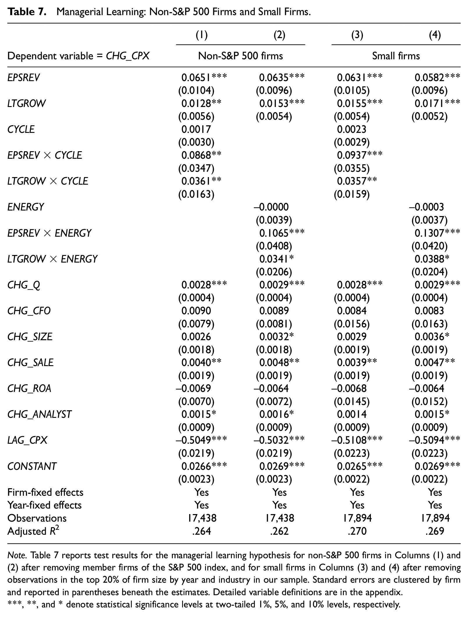
Note. Table 7 reports test results for the managerial learning hypothesis for non-S&P 500 firms in Columns (1) and (2) after removing member firms of the S&P 500 index, and for small firms in Columns (3) and (4) after removing observations in the top 20% of firm size by year and industry in our sample. Standard errors are clustered by firm and reported in parentheses beneath the estimates. Detailed variable definitions are in the appendix.

***

, **, and * denote statistical significance levels at two-tailed 1%, 5%, and 10% levels, respectively.

In Table 7, we find managerial learning in both subsamples. For non-S&P 500 firms in Columns (1) and (2), the coefficients of EPSREV×CYCLE and LTGROW×CYCLE are positive and statistically significant at the .05 levels; the coefficients of EPSREV×ENERGY and LTGROW×ENERGY are positive and statistically significant at the .01 and .10 levels, respectively. In Columns (3) and (4), the results based on small firms are similar to those based on non-S&P 500 firms. These results suggest that our results in Table 3 are not driven by bellwether firms.

Financial Constraints

We also examine the effects of financial constraints, which play an important role in corporate capital investment (e.g., Almeida & Campello, 2007). Financial constraints can affect how corporate investments respond to market signals such as stock prices or analyst forecasts (e.g., Baker et al., 2003). If a firm’s exposure to macroeconomic factors is correlated with its financial constraints,²⁰ this can offer an alternative explanation for our results.

We thus examine whether our results are attributable to the effects of financial constraints. Following Baker et al. (2003), we construct a four-variable version of the Kaplan–Zingales measure, KZ, as a proxy for firms’ degree of equity dependence. KZ is calculated as a weighted sum of cash flow, cash dividends, and cash balances, all scaled by lagged assets and leverage ratio. (A detailed definition of KZ is available in the appendix). We control for KZ and report the regression estimates in Table 8.

Table 8.

Managerial Learning: Controlling for the Effects of Financial Constraints.

Dependent variable = CHG_CPX	(1)	(2)	(3)	(4)
EPSREV	0.0668***	0.0610***	0.0727***	0.0666***
	(0.0096)	(0.0086)	(0.0099)	(0.0095)
LTGROW	0.0141***	0.0162***	0.0166***	0.0187***
	(0.0047)	(0.0044)	(0.0049)	(0.0047)
CYCLE	−0.0001		0.0002
	(0.0023)		(0.0023)
EPSREV×CYCLE	0.0885***		0.0899***
	(0.0313)		(0.0308)
LTGROW×CYCLE	0.0394***		0.0365***
	(0.0135)		(0.0137)
ENERGY		−0.0011		−0.0008
		(0.0030)		(0.0030)
EPSREV×ENERGY		0.1338***		0.1335***
		(0.0386)		(0.0380)
LTGROW×ENERGY		0.0380**		0.0356**
		(0.0171)		(0.0173)
KZ	−0.0035***	−0.0036***	−0.0029***	−0.0029***
	(0.0004)	(0.0004)	(0.0005)	(0.0005)
EPSREV×KZ			−0.0057	−0.0049
			(0.0046)	(0.0049)
LTGROW×KZ			−0.0047*	−0.0053*
			(0.0028)	(0.0028)
CHG_Q	0.0027***	0.0028***	0.0026***	0.0027***
	(0.0003)	(0.0003)	(0.0003)	(0.0003)
CHG_CFO	0.0068	0.0067	0.0063	0.0062
	(0.0073)	(0.0076)	(0.0071)	(0.0074)
CHG_SIZE	0.0007	0.0012	0.0005	0.0009
	(0.0016)	(0.0016)	(0.0016)	(0.0016)
CHG_SALE	0.0039**	0.0045***	0.0035**	0.0041**
	(0.0016)	(0.0016)	(0.0016)	(0.0016)
CHG_ROA	−0.0064	−0.0061	−0.0063	−0.0059
	(0.0066)	(0.0069)	(0.0064)	(0.0066)
CHG_ANALYST	0.0013*	0.0014*	0.0013	0.0013*
	(0.0008)	(0.0008)	(0.0008)	(0.0008)
LAG_CPX	−0.4838***	−0.4824***	−0.4836***	−0.4823***
	(0.0223)	(0.0222)	(0.0223)	(0.0221)
CONSTANT	0.0253***	0.0255***	0.0250***	0.0251***
	(0.0020)	(0.0019)	(0.0020)	(0.0020)
Firm-fixed effects	Yes	Yes	Yes	Yes
Year-fixed effects	Yes	Yes	Yes	Yes
Observations	22,376	22,376	22,376	22,376
Adjusted R²	.269	.269	.270	.270

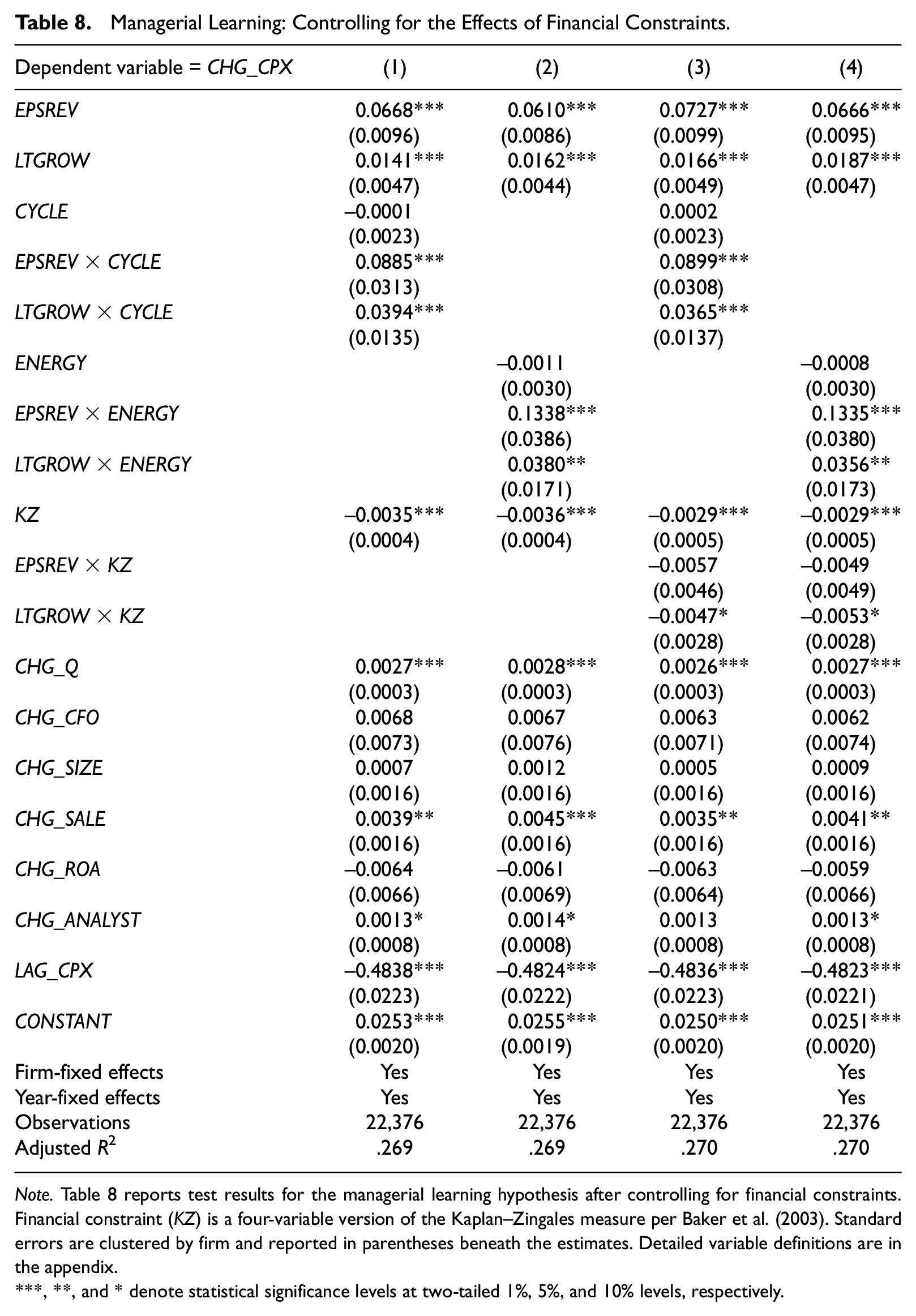
Note. Table 8 reports test results for the managerial learning hypothesis after controlling for financial constraints. Financial constraint (KZ) is a four-variable version of the Kaplan–Zingales measure per Baker et al. (2003). Standard errors are clustered by firm and reported in parentheses beneath the estimates. Detailed variable definitions are in the appendix.

***

, **, and * denote statistical significance levels at two-tailed 1%, 5%, and 10% levels, respectively.

In Table 8 Columns (1) and (2), we control for our proxy for financial constraint, KZ. In Columns (3) and (4), we control for not only KZ but also its interaction with analyst forecasts, EPSREV×KZ and LTGROW×KZ. As expected, KZ has significantly negative effects on capital investments. The coefficients of LTGROW×KZ are negative and significant at the .10 levels, while the coefficients of EPSREV×KZ are not significant. More importantly, even after we include these controls, the coefficients of EPSREV×CYCLE and LTGROW×CYCLE (or ×ENERGY) remain positive and significant, similar to the results in Table 3, suggesting that our results are robust to controlling for the effects of financial constraints.

Investment Efficiency

Our main analyses suggest that managers learn from analyst forecasts when making investment decisions. We complement these tests by examining whether such learning leads to improved investment efficiency. Specifically, we construct a measure of investment efficiency following Goodman et al. (2014) based on a regression of a firm’s capital expenditure on lag Tobin’s Q, cash flow from operations, lag asset growth, and lag capital expenditure. We also measure the extent of managerial learning based on the coefficients of the interaction terms of analyst forecast variables and analyst information advantages in a reduced form of Model (3), estimated for each firm. Untabulated results provide some preliminary evidence that for firms with greater exposure to macroeconomic factors, managers with greater learning from analysts achieve higher investment efficiency.

Conclusion

Our study takes one of the first steps in documenting what managers learn directly from financial analysts’ earnings forecasts and long-term growth forecasts in making investment decisions. We provide evidence consistent with managers learning from analysts about the implications of macroeconomic factors, namely, the business cycle and energy prices, for firm prospects. These results broaden our understanding of the direction of information exchange between managers and analysts and suggest that financial analysts play an important and direct role not only in the information environment of the capital market but also in the real economy. Our results do not preclude the possibility that there are other aspects in analysts’ forecasts, recommendations, or analyst reports that can have important real investment implications. Managers can also learn from other market participants for investment-relevant information. Future research can identify and examine other aspects of analysts’ information advantage or the information advantage of other market participants.

Footnotes

Appendix

Appendix.

Definitions of Variables.

Variable	Definition
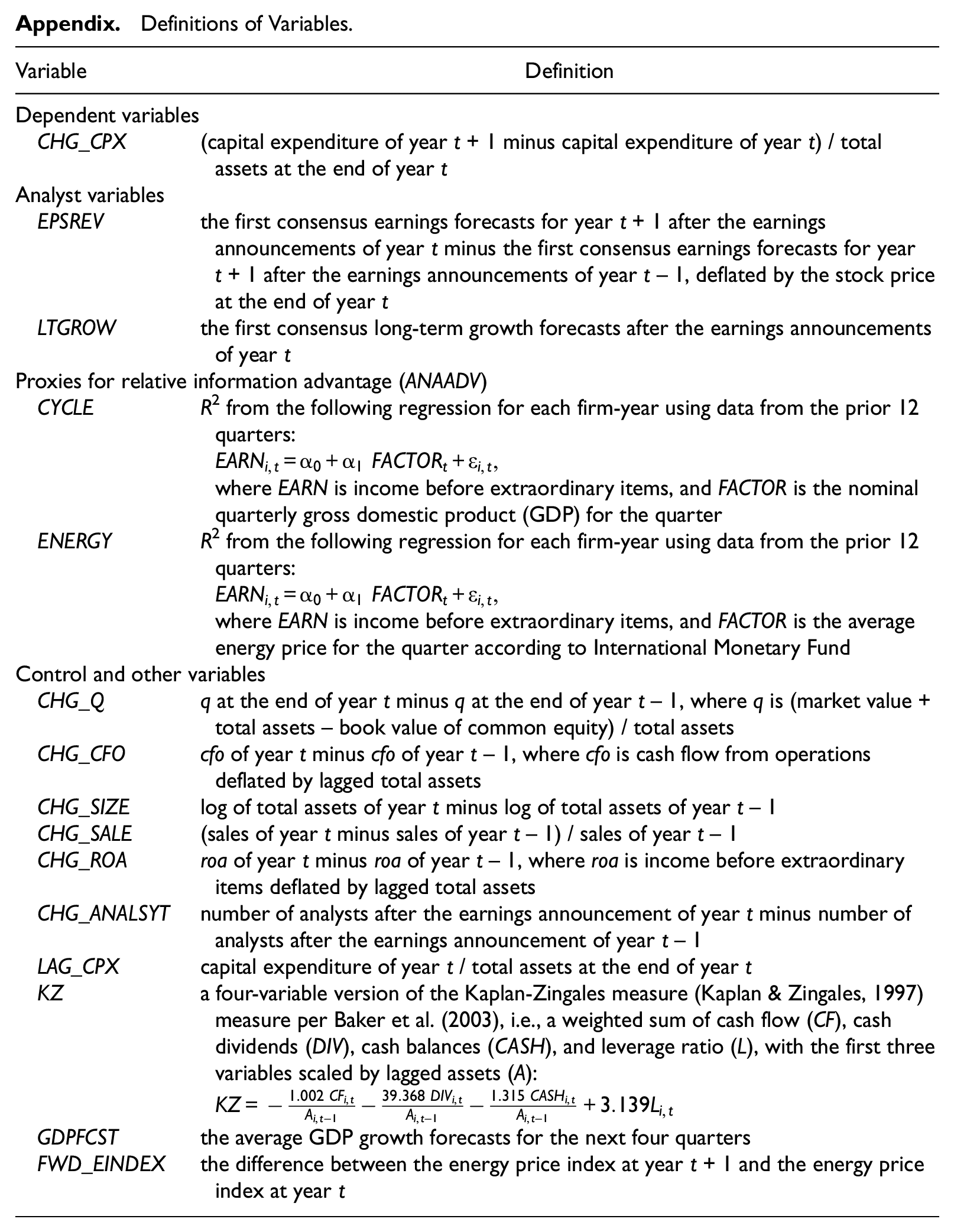
Dependent variables
CHG_CPX	(capital expenditure of year t+ 1 minus capital expenditure of year t) / total assets at the end of year t
Analyst variables
EPSREV	the first consensus earnings forecasts for year t+ 1 after the earnings announcements of year t minus the first consensus earnings forecasts for year t+ 1 after the earnings announcements of year t– 1, deflated by the stock price at the end of year t
LTGROW	the first consensus long-term growth forecasts after the earnings announcements of year t
Proxies for relative information advantage (ANAADV)
CYCLE	R² from the following regression for each firm-year using data from the prior 12 quarters: $EAR N_{i, t} = α_{0} + α_{1} FACTO R_{t} + ε_{i, t},$ where EARN is income before extraordinary items, and FACTOR is the nominal quarterly gross domestic product (GDP) for the quarter
ENERGY	R² from the following regression for each firm-year using data from the prior 12 quarters: $EAR N_{i, t} = α_{0} + α_{1} FACTO R_{t} + ε_{i, t},$ where EARN is income before extraordinary items, and FACTOR is the average energy price for the quarter according to International Monetary Fund
Control and other variables
CHG_Q	q at the end of year t minus q at the end of year t– 1, where q is (market value + total assets – book value of common equity) / total assets
CHG_CFO	cfo of year t minus cfo of year t– 1, where cfo is cash flow from operations deflated by lagged total assets
CHG_SIZE	log of total assets of year t minus log of total assets of year t– 1
CHG_SALE	(sales of year t minus sales of year t– 1) / sales of year t– 1
CHG_ROA	roa of year t minus roa of year t– 1, where roa is income before extraordinary items deflated by lagged total assets
CHG_ANALSYT	number of analysts after the earnings announcement of year t minus number of analysts after the earnings announcement of year t– 1
LAG_CPX	capital expenditure of year t / total assets at the end of year t
KZ	a four-variable version of the Kaplan-Zingales measure (Kaplan & Zingales, 1997) measure per Baker et al. (2003), i.e., a weighted sum of cash flow (CF), cash dividends (DIV), cash balances (CASH), and leverage ratio (L), with the first three variables scaled by lagged assets (A): $KZ = - \frac{1.002 C F_{i, t}}{A_{i, t - 1}} - \frac{39.368 DI V_{i, t}}{A_{i, t - 1}} - \frac{1.315 CAS H_{i, t}}{A_{i, t - 1}} + 3.139 L_{i, t}$
GDPFCST	the average GDP growth forecasts for the next four quarters
FWD_EINDEX	the difference between the energy price index at year t+ 1 and the energy price index at year t

Acknowledgements

We are grateful to Xiao-Jun Zhang (JAAF Editor), Stephanie Larocque (JAAF Associate Editor), and two anonymous reviewers for their helpful comments and suggestions. We thank Qi Chen, Joshua Livnat, Xiaojing Meng, and seminar participants at the Shanghai University of Finance and Economics for their helpful comments. All errors are our own.

Declaration of Conflicting Interests

The author(s) declared no potential conflicts of interest with respect to the research, authorship, and/or publication of this article.

Funding

The author(s) received no financial support for the research, authorship, and/or publication of this article.

ORCID iD

Yaqin Hu

Notes

Author Biographies

Yaqin Hu is an assistant professor of accounting at McMaster University in Canada. Her research interests include financial reporting and voluntary disclosure, SEC regulation, financial analysts, CEO labor market, and litigations.

Yuan Zhang is an associate professor of accounting at the University of Texas at Dallas. Her research interests include financial analysts, financial reporting and voluntary disclosure, and capital market. Her research has been published in top journals such as Journal of Accounting Research, Journal of Accounting and Economics, The Accounting Review, and Management Science. She serves on the editorial board of several accounting journals including The Accounting Review and is an Associate Editor for The Asia-Pacific Journal of Accounting and Economics.

References

Almeida

Campello

(2007). Financial constraints, asset tangibility, and corporate investment. The Review of Financial Studies, 20(5), 1429–1460.

Amiram

Owens

Rozenbaum

(2016). Do information releases increase or decrease information asymmetry? New evidence from analyst forecast announcements. Journal of Accounting and Economics, 62(1), 121–138.

Anilowski

Feng

Skinner

D. J.

(2007). Does earnings guidance affect market returns? The nature and information content of aggregate earnings guidance. Journal of Accounting and Economics, 44(1–2), 36–63.

Bae

Biddle

G. C.

Park

C. W.

(2022). Managerial learning from analyst feedback to voluntary capex guidance, investment efficiency, and firm performance. Management Science, 68(1), 583–607.

Baik

Jiang

(2006). The use of management forecasts to dampen analysts’ expectations. Journal of Accounting and Public Policy, 25(5), 531–553.

Baker

Stein

J. C.

Wurgler

(2003). When does the market matter? Stock prices and the investment of equity-dependent firms. The Quarterly Journal of Economics, 118(3), 969–1005.

Ball

Brown

(1967). Some preliminary findings on the association between the earnings of a firm, its industry, and the economy. Journal of Accounting Research, 5, 55–77.

Ball

Sadka

(2009). Aggregate earnings and asset prices. Journal of Accounting Research, 47(5), 1097–1133.

Barth

M. E.

E. C.

(2014). Non-diversifiable volatility risk and risk premiums at earnings announcements. The Accounting Review, 89(5), 1579–1607.

10.

Bernanke

B. S.

(1983). Irreversibility, uncertainty, and cyclical investment. The Quarterly Journal of Economics, 98(1), 85–106.

11.

Bradshaw

M. T.

(2004). How do analysts use their earnings forecasts in generating stock recommendations? The Accounting Review, 79(1), 25–50.

12.

Brogaard

Shi

Wei

K. C.

You

(2019). Do analysts improve investment efficiency? Journal of Contemporary Accounting and Economics, 16(3), Article 100213.

13.

Chapman

Green

J. R.

(2018). Analysts’ influence on managers’ guidance. The Accounting Review, 93(1), 45–69.

14.

Chen

Xie

Zhang

(2017). How does analysts’ forecast quality relate to corporate investment efficiency? Journal of Corporate Finance, 43, 217–240.

15.

Chen

Goldstein

Jiang

(2007). Price informativeness and investment sensitivity to stock price. The Review of Financial Studies, 20(3), 619–650.

16.

Choi

J. K.

Hann

R. N.

Subasi

Zheng

(2020). An empirical analysis of analysts’ capital expenditure forecasts: evidence from corporate investment efficiency. Contemporary Accounting Research, 37(4), 2615–2648.

17.

Cotter

Tuna

Wysocki

P. D.

(2006). Expectations management and beatable targets: How do analysts react to explicit earnings guidance? Contemporary Accounting Research, 23(3), 593–624.

18.

De Bondt

W. F.

Thaler

R. H.

(1990). Do security analysts overreact? The American Economic Review, 80(2), 52–57.

19.

Dechow

P. M.

Hutton

A. P.

Sloan

R. G.

(2000). The relation between analysts’ forecasts of long-term earnings growth and stock price performance following equity offerings. Contemporary Accounting Research, 17(1), 1–32.

20.

Dessaint

Foucault

Frésard

Matray

(2019). Noisy stock prices and corporate investment. The Review of Financial Studies, 32(7), 2625–2672.

21.

Durnev

Mangen

(2009). Corporate investments: Learning from restatements. Journal of Accounting Research, 47(3), 679–720

22.

Durnev

Mangen

(2020). The spillover effects of MD&A disclosures for real investment: The role of industry competition. Journal of Accounting and Economics, 70(1), 101299.

23.

Easley

O’Hara

Paperman

(1998). Financial analysts and information-based trade. Journal of Financial Markets, 1(2), 175–201.

24.

Edmans

Jayaraman

Schneemeier

(2017). The source of information in prices and investment-price sensitivity. Journal of Financial Economics, 126(1), 74–96.

25.

Erickson

Whited

T. M.

(2000). Measurement error and the relationship between investment and q. Journal of Political Economy, 108(5), 1027–1057.

26.

Ferracuti

Stubben

S. R.

(2019). The role of financial reporting in resolving uncertainty about corporate investment opportunities. Journal of Accounting and Economics, 68(2–3), Article 101248.

27.

Foucault

Frésard

(2014). Learning from peers’ stock prices and corporate investment. Journal of Financial Economics, 111(3), 554–577.

28.

Gao

Liang

P. J.

(2013). Informational feedback, adverse selection, and optimal disclosure policy. Journal of Accounting Research, 51(5), 1133–1158.

29.

Gilchrist

Zakrajšek

(2012). Credit spreads and business cycle fluctuations. American Economic Review, 102(4), 1692–1720.

30.

Gilson

S. C.

Healy

P. M.

Noe

C. F.

Palepu

K. G.

(2001). Analyst specialization and conglomerate stock breakups. Journal of Accounting Research, 39(3), 565–582.

31.

Goldstein

Yang

(2017). Information disclosure in financial markets. Annual Review of Financial Economics, 9, 101–125.

32.

Goodman

T. H.

Neamtiu

Shroff

White

H. D.

(2014). Management forecast quality and capital investment decisions. The Accounting Review, 89(1), 331–365.

33.

Chen

(2004). Analysts’ treatment of nonrecurring items in street earnings. Journal of Accounting and Economics, 38, 129–170.

34.

Hann

R. N.

Kim

Zheng

(2019). Intra-industry information transfers: Evidence from changes in implied volatility around earnings announcements. Review of Accounting Studies, 24(3), 927–971.

35.

Hayek

F. A.

(1945). The use of knowledge in society. The American Economic Review, 35(4), 519–530.

36.

J. J.

Tian

(2013). The dark side of analyst coverage: The case of innovation. Journal of Financial Economics, 109(3), 856–878.

37.

Hugon

Kumar

Lin

A. P.

(2016). Analysts, macroeconomic news, and the benefit of active in-house economists. The Accounting Review, 91(2), 513–534.

38.

Hutton

A. P.

Lee

L. F.

Shu

S. Z.

(2012). Do managers always know better? The relative accuracy of management and analyst forecasts. Journal of Accounting Research, 50(5), 1217–1244.

39.

Jayaraman

Shuang Wu

(2020). Should I stay or should I grow? Using voluntary disclosure to elicit market feedback. The Review of Financial Studies, 33(8), 3854–3888.

40.

Kaplan

S. N.

Zingales

(1997). Do investment-cash flow sensitivities provide useful measures of financing constraints? The Quarterly Journal of Economics, 112(1), 169–215.

41.

(2006). The effect of issuing biased earnings forecasts on analysts’ access to management and survival. Journal of Accounting Research, 44(5), 965–999.

42.

Kim

Pandit

Wasley

C. E.

(2016). Macroeconomic uncertainty and management earnings forecasts. Accounting Horizons, 30(1), 157–172.

43.

Langberg

Sivaramakrishnan

(2008). Voluntary disclosures and information production by analysts. Journal of Accounting and Economics, 46(1), 78–100.

44.

Langberg

Sivaramakrishnan

(2010). Voluntary disclosures and analyst feedback. Journal of Accounting Research, 48(3), 603–646.

45.

Luo

(2005). Do insiders learn from outsiders? Evidence from mergers and acquisitions. The Journal of Finance, 60(4), 1951–1982.

46.

Merkley

K. J.

Bamber

L. S.

Christensen

T. E.

(2013). Detailed management earnings forecasts: Do analysts listen? Review of Accounting Studies, 18(2), 479–521.

47.

Piotroski

J. D.

Roulstone

D. T.

(2004). The influence of analysts, institutional investors, and insiders on the incorporation of market, industry, and firm-specific information into stock prices. The Accounting Review, 79(4), 1119–1151.

48.

Ramalingegowda

Wang

C. S.

(2013). The role of financial reporting quality in mitigating the constraining effect of dividend policy on investment decisions. The Accounting Review, 88(3), 1007–1039.

49.

Richardson

Teoh

S. H.

Wysocki

P. D.

(2004). The walk-down to beatable analyst forecasts: The role of equity issuance and insider trading incentives. Contemporary Accounting Research, 21(4), 885–924.

50.

Roychowdhury

Shroff

Verdi

R. S.

(2019). The effects of financial reporting and disclosure on corporate investment: A review. Journal of Accounting and Economics, 68(2–3), Article 101246.

51.

Sharpe

S. A.

(2005). How does the market interpret analysts’ long-term growth forecasts? Journal of Accounting, Auditing & Finance, 20(2), 147–166.

52.

Shroff

(2017). Corporate investment and changes in GAAP. Review of Accounting Studies, 22(1), 1–63.

53.

Stern

D. I.

(2018). Energy-GDP relationship. In Vernengo

Caldentey

E. P.

Rosser

B. J.

Jr. (Eds.), The new Palgrave dictionary of economics (pp. 3697–3714). Springer.

54.

Zhang

(2008). Analyst responsiveness and the post-earnings-announcement drift. Journal of Accounting and Economics, 46(1), 201–215.

Analyst Forecasts,Managerial Learning,and Corporate Investment

Abstract

Keywords

Introduction

Variable Measurement and Research Design

Analyst Information

Analyst Information Advantage on Macroeconomic Factors

Research Design

Sample and Descriptive Statistics

Empirical Results

Investment-Forecast Sensitivity

Managerial Learning From Analysts

Analyst Information Advantage

Effects of Firm Capital Intensity

Alternative Explanations and Tests

Investment Sensitivity to Macroeconomic Factors

Bellwether Firms

Financial Constraints

Investment Efficiency

Conclusion

Footnotes

Appendix

Acknowledgements

Declaration of Conflicting Interests

Funding

ORCID iD

Notes

Author Biographies

References