Specific Absorbed Fractions for Reference Paediatric Individuals

Abstract

The calculation of doses to organs and tissues of interest due to internally emitting radionuclides requires knowledge of the time-dependent distribution of the radionuclide, its physical decay properties, and the fraction of emitted energy absorbed per mass of the target. The latter property is quantified as the specific absorbed fraction (SAF). This publication provides photon, electron, alpha particle, and neutron (for nuclides undergoing spontaneous fission) SAF values for the suite of reference individuals. The reference individuals are defined largely by information provided in ICRP Publication 89. Some improvements and additional data are provided in this publication which define the reference individual’s source and target region masses used in the Occupational Intake of Radionuclides (OIR) and Dose Coefficients for Intakes of Radionuclides by Members of the Public series of publications. The set of reference individuals includes males and females at 0 (newborn), 1, 5, 10, 15, and 20 (adult) years of age. The reference adult masses and SAFs provided in this publication are identical to those in ICRP Publication 133 and those used in the OIR series of publications. Computation of SAF values involves simulating radiation transport in computational models which represent the geometry of the reference individuals. The reference voxel phantoms of ICRP Publication 143 are used for photon and neutron transport, and most electron transport. Alpha particle transport is not necessary for large tissue regions as the short range allows for an assumption of full energy absorption (absorbed fraction of unity) for self-irradiation geometries. Additional computational models are needed for charged particles in small, overlapping, or interlaced geometries. Stylised models are described and used for electrons and alpha particles in the alimentary and respiratory tract regions. Image-based models are used to compute SAFs for charged particles within the skeleton. This publication is accompanied by an electronic supplement which includes files containing SAFs for each radiation type in each reference individual. The supplement also includes source and target region masses for each reference individual, as well as skeletal dose–response functions for photons incident upon the skeleton.

© 2024 ICRP. Published by SAGE.

MAIN POINTS

Specific absorbed fraction (SAF) values are provided for International Commission on Radiological Protection male and female reference individuals at 0, 1, 5, 10, 15, and 20 years of age for internally emitted photons, electrons, alpha particles, and fission-spectrum neutrons associated with radionuclides which decay by spontaneous fission.

Source and target region masses for the reference individuals consistent with these SAF values are tabulated and their origins defined.

SAF values and source and target region masses for the adults are the same as those in Publication 133 (ICRP, 2016a) and utilised in the Occupational Intake of Radionuclides series of publications (ICRP, 2015, 2016b, 2017, 2019, 2022).

Computational models used to obtain energy absorption data include the reference voxel phantoms of Publication 143 (ICRP, 2020b), stylised models for charged particles in intrarespiratory and intra-alimentary tract geometries, and image-based models for charged particles emitted within the skeleton.

In forthcoming publications, the reference SAFs presented in this publication will be coupled with the nuclear decay data of Publication 107 (ICRP, 2008b) and the biokinetic models describing temporal distribution of radionuclide activity to calculate reference dose coefficients to members of the public and dose to patients from radiopharmaceuticals.

In addition to photons, energy-dependent SAFs for electrons and alpha particles are provided, representing a significant improvement in radiation protection dosimetry compared with the non-energy-dependent SAFs in Publication 30 (ICRP, 1979).

1. Introduction

(1) Publication 103 (ICRP, 2007) describes the latest revisions to the radiation protection quantities, equivalent and effective dose. Since issued, Committee 2 of the International Commission on Radiological Protection (ICRP) has been involved in an effort to publish dose coefficients for external (ICRP, 2010, 2013, 2020c) and internal exposures. Specific absorbed fractions (SAFs) are required in the ICRP methodology for computing internal dose coefficients. Publication 133 (ICRP, 2016a) contains the SAFs for the reference adults utilised in computing the dose coefficients of the Occupational Intake of Radionuclides (OIR) series (ICRP, 2015, 2016b, 2017, 2019, 2022). This publication provides SAFs for members of the public, including children. These SAFs will be used in the computation of internal dose coefficients in the forthcoming Dose Coefficients for Intakes of Radionuclides by Members of the Public (EIR) series.

(2) The computation of internal dose coefficients first requires definition of the individuals for whom the dose coefficients are being computed. A group of 12 reference individuals are defined – males and females aged 0 (newborn), 1, 5, 10, 15, and 20 (adult) years. The definition of the tissue masses comes largely from Publication 89 (ICRP, 2002). In this publication, these masses are restated and expanded upon or replaced when appropriate.

(3) The SAF is defined as the fraction of energy emitted within a source region which is absorbed in a target region per mass of the target region. Target regions may be whole organs or tissue layers. Source regions may be whole organs, tissue regions, surfaces, contents of hollow organs, or distributed around the body in the case of a blood source. To compute the fractional energy absorption, a series of reference computational phantoms and models provide a representative geometry for radiation transport calculations. Reference voxel phantoms (ICRP, 2009, 2020b) are used for many of the source-target geometries. Additional computational models provide the intricate geometry needed for charged particle transport in smaller, overlapping, or interlaced source and target regions within the alimentary tract, respiratory tract, and skeleton. While the phantoms and models were designed with Publication 89 (ICRP, 2002) in mind, they are constructs of theoretical anatomical geometries. For a variety of reasons, the masses of regions in the phantoms or models may not match the reference individual definitions exactly. In such cases, adjustments are made to phantom/model SAFs to derive appropriate reference SAFs.

(4) The masses provided in Table 2.8 of Publication 89 (ICRP, 2002) provide reference values for the masses for each age and sex. Importantly, the masses of the organs and tissues in this table, unless noted specifically, do not include the contribution from blood perfusing organs and tissues. Rather, Table 2.8 generally provides the masses of the organ and tissue parenchyma. To arrive at an organ or tissue mass inclusive of the perfused blood, a blood distribution model must be coupled to the masses in Table 2.8. Section 3.2 of this publication describes in detail how such masses are computed.

(5) The reference voxel phantoms in Publications 110 and 143 (ICRP, 2009, 2020b) were designed based on the parenchyma masses in Table 2.8 of Publication 89 (ICRP, 2002). As a result, organs and tissues in the reference voxel phantoms are generally smaller than desired due to the missing contribution from perfused blood. Section 5.1 of this publication describes how and which SAFs were adjusted from values computed in reference voxel phantoms to be consistent with target masses inclusive of blood (provided in Section 3.3) Note that the reference adult mesh-type phantoms in Publication 145 (ICRP, 2020a) did account for the contribution of perfused blood. Forthcoming mesh-type phantoms for reference paediatric individuals will also include the contribution of perfused blood in tissue. However, the mesh-type phantoms were not available at the time Monte Carlo transport simulations supporting this publication were performed, and therefore the reference voxel phantoms were used, as described in Section 4.1.

(6) The SAFs for the reference adults were provided in Publication 133 (ICRP, 2016a). As they are also used in the EIR series and radiopharmaceutical dosimetry, adult SAFs have been included in this publication for ease of access. The adult SAFs do not differ from those used in the OIR series.

2. ICRP Schema for Internal Dose Assessment

(7) Doses to members of the public may result from environmental exposure to radionuclides. If such a radionuclide is inhaled or ingested, the potential exists for it to be transferred to the blood and incorporated into tissue, thereby creating a source of radiation emissions internal to the body. The resulting dose from an intake of radioactive material takes place over an extended period of time, with the extent depending on the physical properties of the nucleus and physiological properties of the chemical form of the material.

(8) The methods described in this section will be used to compute internal dose coefficients for members of the public. Internal dose coefficients provide the dose per unit intake activity. Depending on the interest, the coefficient could provide equivalent dose to a specific target tissue or effective dose.

(9) The methodology is similar to that presented in the OIR series of publications (ICRP, 2015, 2016a,b, 2017, 2019, 2022), with an important difference in the handling of age. In the OIR series, dose calculations were performed for the reference adults alone. As parameters associated with the reference adults are constant with age, determining the dose delivered over time involved simple integration of the activity term. The energy absorption term (S-coefficient) for the reference adults is time invariant.

(10) The EIR series, however, includes dose coefficients for intakes occurring as children. Unless the radionuclide’s physical or biological removal from the body is very fast, growth of the child should be considered. For these individuals, both the activity term and the energy absorption term vary with time. The section below describes these terms, and how their time-variant nature needs to be handled in computing internal dose coefficients.

(11) The methodology presented here can also be applied to patients in diagnostic nuclear medicine. For such patients, organ absorbed dose coefficients would be the desired quantity, rather than equivalent dose coefficients. Finally, the caveat described in Section 2.2.1 applies to patient dosimetry.

2.1. Methodology for dose calculations

(12) The ICRP dosimetry system is presented below as applied to assessment of organ equivalent dose and effective dose following intakes of radionuclides. The system involves numerical solution of reference biokinetic models, yielding the time-dependent activity in various source tissues. These solutions are then coupled with reference data on nuclear decay information and SAFs.

2.1.1. Computational solutions to the ICRP reference biokinetic models

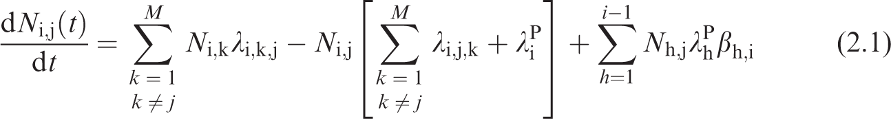
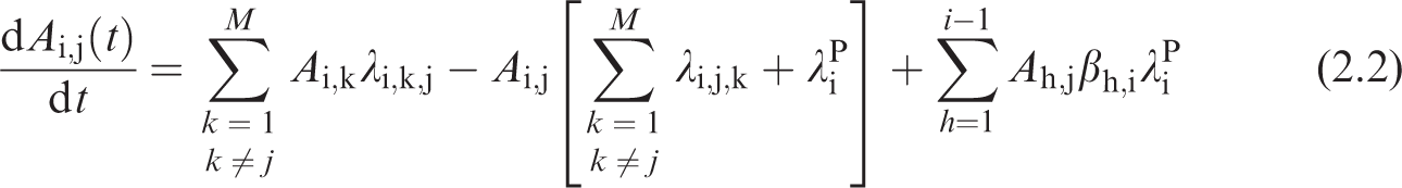
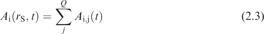
(13) The Human Respiratory Tract Model (HRTM), the Human Alimentary Tract Model (HATM), and the systemic biokinetic models describe the dynamic behaviour of radionuclide movement within the body. Given the route(s) of intake, these models predict the subsequent uptake to the systemic circulation, the distribution among tissues of the body, and the routes of elimination from the body. The physical decay of the radionuclide and its radioactive progeny are also modelled. The result is a coupled system of first-order differential equations. The solution to the set of equations is the time-dependent distribution of the radionuclide and its radioactive progeny in mathematical compartments associated with anatomical regions in the body.

(14) N_i,j(t) represents the number of nuclides of radionuclide i in compartment j at time t. The rate of change of the number of nuclides i of the decay chain, i = 1, 2, …, n with i = 1 being the parent nuclide taken into the body, is given in Eq. (2.1). Note that in addition to the number of nuclei terms, the biokinetic transfer rates may also vary with age and are therefore functions of time. The function of time notation $\left(t\right)$ has been omitted from these quantities on the right-hand side of Eq. (2.1) to improve readability:

$$\frac{\text{d}{N}_{\mathrm{i},\mathrm{j}}\left(t\right)}{\text{d}t}=\sum _{\begin{array}{c}k=1\\ k\ne j\end{array}}^M{N}_{\mathrm{i},\mathrm{k}}{\lambda }_{\mathrm{i},\mathrm{k},\mathrm{j}}-N_{\mathrm{i},\mathrm{j}}\left[\sum _{\begin{array}{c}k=1\\ k\ne j\end{array}}^M{\lambda }_{\mathrm{i},\mathrm{j},\mathrm{k}}+{\lambda }_{\mathrm{i}}^{\mathrm{P}}\right]+\sum _{h=1}^{i-1}{N}_{\mathrm{h},\mathrm{j}}{\lambda }_{\mathrm{h}}^{\mathrm{P}}{\beta }_{\mathrm{h},\mathrm{i}}$$

(2.1)

where M is the number of compartments describing the kinetics; $N_{\mathrm{i},\mathrm{k}}$ is the number of nuclei of chain member i in donor compartment k and varies with time; λ_i,j,k is the fractional transfer rate of chain member i from compartment j (donor compartment) to compartment k (receiving compartment) in the biokinetic model and may vary with time (age); ${\lambda }_{\mathrm{i}}^{\mathrm{p}}$ is the physical decay constant of chain member i; $N_{\mathrm{h},\mathrm{j}}$ is the number of nuclei of precursor nuclide h in compartment j and varies with time; ${\lambda }_{\mathrm{h}}^{\mathrm{P}}$ is the physical decay constant of precursor chain member h; and β_h,i is the fraction of the decays of chain member h forming member i.

• (15) Given the initial conditions specified for the compartments, N_i,j(0), Eq. (2.1) defines the dynamic behaviour of the radionuclide and its progeny within the human body. The first term on the right-hand side of Eq. (2.1) represents the rate of flow of chain member i into compartment j from all donor compartments. The second term represents the rate of removal of member i from compartment j both by transfer to receiving compartments and by physical decay. The third term addresses the ingrowth of member i within compartment j due to the presence of its precursors h in the compartment. The number of nuclei of the precursor multiplied by its physical decay is the activity of the precursor, $A_{\mathrm{h},\mathrm{j}}$ . Note that the members of the decay chain are assumed to be of order such that the precursors of member i have indexes less than i. An ordered listing of the chain members can be obtained using the DECDATA software distributed with Publication 107 (ICRP, 2008b).

• (16) If all terms in Eq. (2.1) are multiplied by the physical decay constant of the chain member being considered, ${\lambda }_{\mathrm{i}}^{\mathrm{P}}$ , the rate of change of the activity of chain member i in compartment j is obtained as shown in Eq. (2.2):

  $$\frac{\text{d}{A}_{\mathrm{i},\mathrm{j}}\left(t\right)}{\text{d}t}=\sum _{\begin{array}{c}k=1\\ k\ne j\end{array}}^M{A}_{\mathrm{i},\mathrm{k}}{\lambda }_{\mathrm{i},\mathrm{k},\mathrm{j}}-A_{\mathrm{i},\mathrm{j}}\left[\sum _{\begin{array}{c}k=1\\ k\ne j\end{array}}^M{\lambda }_{\mathrm{i},\mathrm{j},\mathrm{k}}+{\lambda }_{\mathrm{i}}^{\mathrm{P}}\right]+\sum _{h=1}^{i-1}{A}_{\mathrm{h},\mathrm{j}}{\beta }_{\text{h},\mathrm{i}}{\lambda }_{\mathrm{i}}^{\mathrm{P}}$$

  (2.2)

• (17) The system of n × M ordinary first-order differential equations is solved using suitable numerical methods, under the assumption that A_i,j(0) = 0 for all compartments with the exception of compartments of intake, where non-zero initial conditions are only applied to the parent nuclide (i.e. i = 1). Information on the physical decay constants and branching fraction, ${\beta }_{\mathrm{k},\mathrm{i}}$ , are available in Publication 107 (ICRP, 2008b).

• (18) To calculate the numerical values of the dose coefficients, it is necessary to associate the biokinetic compartments of Eq. (2.2) with anatomical source regions indexed by r_S. A source region may or may not be a living tissue (e.g. the stomach contents may be a source region but are not a living tissue), and may consist of more than one biokinetic compartment. The time-dependent activity in source region r_S is the sum of the time-dependent activity in each biokinetic compartment j comprising the source region:

  $$A_{\mathrm{i}}(r_{\text{S}},t)=\sum _j^Q{A}_{\mathrm{i},\mathrm{j}}\left(t\right)$$

  (2.3)

where Q represents the total number of compartments comprising the source region being considered.

(19) For intakes in reference adults, dosimetric quantities are invariant with time, and it is convenient to integrate the activity in Eq. (2.3) over the 50-year commitment period to obtain the total number of nuclear transformations, as in the OIR series (ICRP, 2015). For intakes in reference children, the dosimetric quantities vary as the reference individual ages. The integration must then wait until after the time-varying activity is multiplied by a time-varying dose per nuclear transformation (S-coefficient).

(20) Dividing the activity in Eq. (2.3) by the total intake activity gives the rate of nuclear transformations per activity intake, $a_{\mathrm{i}}\left(r_{\mathrm{S}},t\right)$ :

$$a_{\mathrm{i}}(r_{\text{S}},t)=\frac{A_{\mathrm{i}}(r_{\text{S}},t)}{A_{\mathrm{exhaled,0}}+\sum j{A}_{\mathrm{i},\mathrm{j}}\left(0\right)}$$

(2.4)

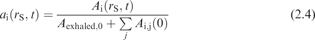
where the denominator includes the prompt exhaled activity $A_{\text{exhaled,0}}$ (pertinent for inhalations, as only a fraction of the intake activity is deposited in the compartments of the HRTM) and the summation of parent activity (i = 1) in all compartments at t = 0. Note that in Publication 130 (ICRP, 2015), the denominator was erroneously described as excluding this exhaled activity. This error was corrected in Publication 133 (ICRP, 2016a). The denominator in Eq. (2.4) has been updated in this publication to be consistent with the description in Publication 133 (ICRP, 2015).

2.1.2. Computation of the ICRP reference dose coefficients for organ equivalent dose

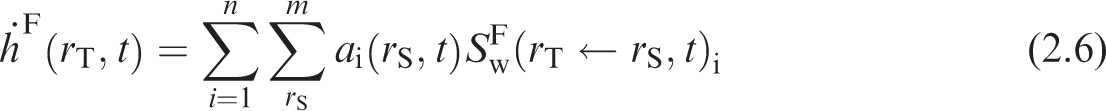
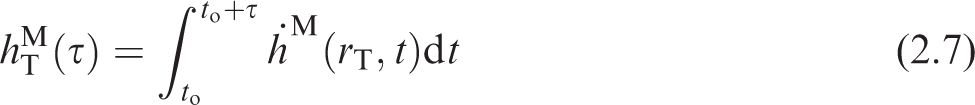
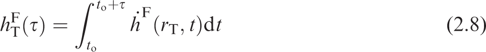
(21) The equivalent dose rate coefficients in target region r_T of the reference adult male, ${\dot{h}}^{\mathrm{M}}\left(r_{\mathrm{T}},t\right),\mathrm{ }$ and the reference adult female, ${\dot{h}}^{\mathrm{F}}(r_{\mathrm{T}},t)$ , are given by:

$${\dot{h}}^{\mathrm{M}}(r_{\mathrm{T}},t)=\sum _{i=1}^n\sum _{r_{\mathrm{S}}}^m{a}_{\mathrm{i}}\left(r_{\mathrm{S}},t\right)S_{\mathrm{w}}^{\mathrm{M}}(r_{\mathrm{T}}\leftarrow r_{\mathrm{S}}{,t)}_{\mathrm{i}}$$

(2.5)

$${\dot{h}}^{\mathrm{F}}(r_{\mathrm{T}},t)=\sum _{i=1}^n\sum _{r_{\mathrm{S}}}^m{a}_{\mathrm{i}}\left(r_{\mathrm{S}},t\right)S_{\mathrm{w}}^{\mathrm{F}}(r_{\mathrm{T}}\leftarrow r_{\mathrm{S}}{,t)}_{\mathrm{i}}$$

(2.6)

The S-coefficients, $S_{\mathrm{w}}^{\mathrm{M}}(r_{\mathrm{T}}\leftarrow r_{\mathrm{S}},t{)}_{\mathrm{i}}$ and $S_{\mathrm{w}}^{\mathrm{F}}(r_{\mathrm{T}}\leftarrow r_{\mathrm{S}}{,t)}_{\mathrm{i}},$ give the radiation weighted equivalent dose in target region $r_{\mathrm{T}}$ per nuclear transformation (Sv Bq⁻¹ s⁻¹) of chain member i (of n members in the chain) in a source region $r_{\mathrm{S}}$ (of m source regions) for the male and female reference individuals, respectively.

• (22) The committed equivalent dose coefficients in each target region are given by integrating the time-dependent equivalent dose rate coefficients over the commitment period as shown in Eqs (2.5) and (2.6), where $t_{\mathrm{o}}$ is the age at intake and $\tau$ is the commitment period:

  $$h_{\mathrm{T}}^{\mathrm{M}}\left(\tau \right)={\int }_{t_{\mathrm{o}}}^{t_{\mathrm{o}}+\tau }{\dot{h}}^{\mathrm{M}}(r_{\mathrm{T}},t)\text{d}t$$

  (2.7)
  $$h_{\mathrm{T}}^{\mathrm{F}}\left(\tau \right)={\int }_{t_{\mathrm{o}}}^{t_{\mathrm{o}}+\tau }{\dot{h}}^{\mathrm{F}}(r_{\mathrm{T}},t)\text{d}t$$

  (2.8)

• (23) Dose coefficients resulting from occupational intakes of radionuclides were published in the OIR series based on a commitment period of 50 years in the reference adults. In the EIR series, committed dose coefficients are computed for reference individuals based on intakes at 3 months, 1 year, 5 years, 10 years, 15 years, and adult. For these individuals, the commitment period is 50 years for intakes as an adult and through age 70 years for intakes at all other ages. The age at intake for the adult may be 20 or 25 years depending on the biokinetics of the considered radionuclide (for skeletal-seeking radionuclides, adult maturity is defined as 25 years of age). Regardless of the age at intake for the adult, the commitment period for the adult is 50 years. In the OIR series of publications, all quantities contributing to the S-coefficient calculation are invariant with respect to time as the reference workers are adults from the time of intake throughout the entire commitment period. As a result, only the activity content in source regions required integration over time, and yielded the total number of nuclear transformations taking place during the commitment period. In the EIR series, this remains true for intakes by the reference adult. For children, however, the SAF varies with respect to time as the child grows and the shape, volume, mass, and distance between tissues changes.

• (24) A number of target tissues are represented by a single target region $r_{\mathrm{T}}$ . In cases where more than one tissue region defines the target tissue, fractional weighting of the equivalent dose must be made. The committed equivalent dose coefficients for tissue T in the reference adult male, $h_{\mathrm{T}}^{\mathrm{M}}\left(\tau \right)$ , and reference adult female, $h_{\mathrm{T}}^{\mathrm{F}}\left(\tau \right)$ , are thus given in Eqs (2.9) and (2.10) as:

  $$h_{\mathrm{T}}^{\mathrm{M}}\left(\tau \right)=\sum _{r_{\mathrm{T}}}f\left(r_{\mathrm{T}},T\right)\mathrm{ }{h}^{\mathrm{M}}(r_{\mathrm{T}},\tau )$$

  (2.9)
  $$h_{\mathrm{T}}^{\mathrm{F}}\left(\tau \right)=\sum _{r_{\mathrm{T}}}f\left(r_{\mathrm{T}},T\right)\mathrm{ }{h}^{\mathrm{F}}(r_{\mathrm{T}},\tau )$$

  (2.10)

where the target region fractional weights, $f\left(r_{\mathrm{T}},T\right),$ are the proportions of the equivalent dose in tissue T associated with target region $r_{\mathrm{T}}$ . With the exception of the target tissues addressed in Table 2.1, the target tissues of Table 2.2 are represented by a single target region, and thus for these tissues $f\left(r_{\mathrm{T}},T\right)$  = 1. In Table 2.1, values of $f\left(r_{\mathrm{T}},T\right)$ for the extrathoracic (ET) and thoracic (TH or lung) regions are taken to be equivalent to their risk apportionment factors as assigned in the revised HRTM. These are assumed to be the same for children in the absence of information (ICRP, 1995a). For the colon, values of $f\left(r_{\mathrm{T}},T\right)$ are taken to be the fractional masses of the stem cell layers within the alimentary tract walls [see Table 7.8 of Publication 100 (ICRP, 2006)]. Sugiyama et al. (2020) found that excess relative risks among a cohort of atomic bomb survivors were not significantly different for proximal and distal colon cancer. The same study found no variation in risk by age at exposure. For the lymphatic nodes, values of $f\left(r_{\mathrm{T}},T\right)$ are taken to be the fractional masses of lymphatic nodes (not lymphatic tissues) within the ET, TH, and non-respiratory regions, consistent with data given previously in Publication 66 (ICRP, 1994). These values are independent of the age of the reference individual.

Table 2.1.

Target region fractional weights [ f (r_T,T)].

Tissue, T	Target region, rT	f (rT,T)
ET	ET1	0.001
	ET2	0.999
Lungs	BB*	1/3
	bb	1/3
	AI	1/3
Colon	Right colon	0.4
	Left colon	0.4
	Rectosigmoid	0.2
Lymphatic nodes	LNET	0.08
	LNTH	0.08
	Lymph (systemic)	0.84

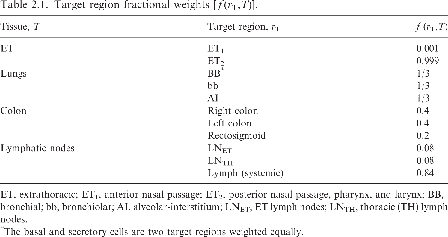
ET, extrathoracic; ET₁, anterior nasal passage; ET₂, posterior nasal passage, pharynx, and larynx; BB, bronchial; bb, bronchiolar; AI, alveolar-interstitium; LN_ET, ET lymph nodes; LN_TH, thoracic (TH) lymph nodes.

^*The basal and secretory cells are two target regions weighted equally.

2.1.3. Computation of the ICRP reference dose coefficients for effective dose

(25) As defined in Publication 103 (ICRP, 2007), the committed effective dose coefficient, e(τ), is:

$$e\left(\tau \right)= \sum _T{w}_{\mathrm{T}\mathrm{ }}\left[\frac{h_{\mathrm{T}}^{\mathrm{M}}\left(\tau \right)+h_{\mathrm{T}}^{\mathrm{F}}\left(\tau \right)}{2}\right]$$

(2.11)

where $w_{\mathrm{T}}$ is the tissue weighting factor for tissue T of Table 2.2, and $h_{\mathrm{T}}^{\mathrm{M}}\left(\tau \right)$ and $h_{\mathrm{T}}^{\mathrm{F}}\left(\tau \right)$ are the corresponding committed equivalent dose coefficients for these same tissues in reference male and female, respectively. The tissue weighting factor for the remainder tissues is applied to the arithmetic mean of the equivalent doses to the 13 tissues for each sex.

Table 2.2.

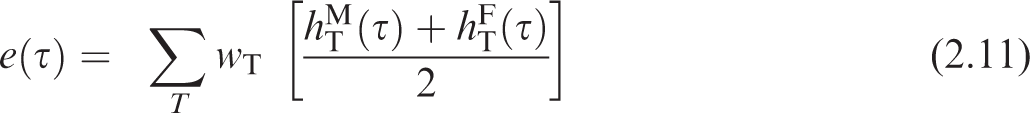
Publication 103 (ICRP, 2007) tissue weighting factors ( $w_{\mathrm{T}}$ ).

Tissue	w T	∑wT
Bone marrow, breast, colon, lung, stomach, remainder tissues (13 for each sex*)	0.12	0.72
Gonads	0.08	0.08
Urinary bladder, oesophagus, liver, thyroid	0.04	0.16
Bone surface, brain, salivary glands, skin	0.01	0.04

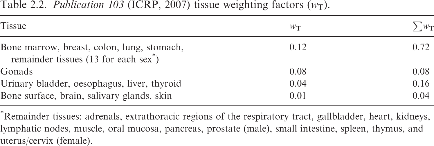
^*Remainder tissues: adrenals, extrathoracic regions of the respiratory tract, gallbladder, heart, kidneys, lymphatic nodes, muscle, oral mucosa, pancreas, prostate (male), small intestine, spleen, thymus, and uterus/cervix (female).

2.2. S-coefficients and the specific absorbed fraction

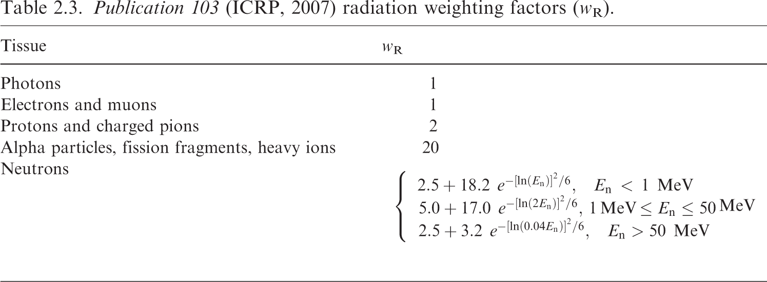
(26) The radiation weighted S-coefficient is the equivalent dose to a target tissue per nuclear transformation taking place in a source region. The S-coefficient is computed as shown in Eq. (2.12) and incorporates nuclear decay data, radiation weighting factor, and SAF, $\mathrm{\Phi }\left(r_{\text{T}}\leftarrow r_{\text{S}},E_{\text{R,i}},t\right)$ :

$$S_{\text{w}}\left(r_{\text{T}}\leftarrow r_{\text{S}},t\right)=\sum _R{w}_{\text{R}}\sum _i{E}_{\text{R,i}}{ Y}_{\text{R,i}}\mathrm{ }\mathrm{\Phi }\left(r_{\text{T}}\leftarrow r_{\text{S}},E_{\text{R,i}},t\right)$$

(2.12)

The energy and yield of the $i$ th emission of radiation type $R$ are denoted by $E_{\text{R,i}}$ and $Y_{\text{R,i}},$ and are tabulated in Publication 107 (ICRP, 2008b). For the continuous energy spectrum associated with beta emissions, an integral is required rather than a summation, as shown in Eq. (2.13):

$$S_{\text{w-beta}}\left(r_{\text{T}}\leftarrow r_{\text{S}},t\right)={\int }_{i=0}^{i_{\text{max}} }{w}_{\text{R}} E_{\text{R,i}}{ Y}_{\text{R,i}}\left(E_{\text{R,i}}\right)\mathrm{ }\mathrm{\Phi }\left(r_{\text{T}}\leftarrow r_{\text{S}},E_{\text{R,i}},t\right)\text{d}{E}_{\text{R}}$$

(2.13)

• (27) In practice, it is necessary to compute the beta contribution given by Eq. (2.13) from the S-coefficient separately from the contribution due to other radiation types. The two contributions are simply summed to give the total S-coefficient for all emissions from a particular radionuclide.

• (28) The radiation weighting factors, $w_{\mathrm{R}}$ , were provided in Publication 103 (ICRP, 2007), and are found in Table 2.3.

• (29) The SAF, $\mathrm{\Phi }$ , is defined in Eq. (2.14) as the fraction of energy, $E_{\text{R}}$ , emitted from a source region, $r_{\text{S}}$ , which is absorbed in a target region, $r_{\text{T}}$ , per mass of the target region, $m_{\text{T}}$ . The absorbed fraction term, $\varphi$ , is a function of the source-target geometry and the energy of radiation type $R$ :

  $$\mathrm{\Phi }\left(r_{\text{T}}\leftarrow r_{\text{S}},E_{\text{R}}\right)=\frac{\varphi \left(r_{\text{T}}\leftarrow r_{\text{S}},E_{\text{R}}\right)}{m_{\text{T}}}$$

  (2.14)

• (30) The absorbed fraction is calculated by radiation transport simulation in voxel phantoms or other geometrical models, as described in Section 4. To calculate a SAF corresponding to the phantom or model, the absorbed fraction is divided by the target mass in that phantom or model. If the target mass represented within the phantom or model is not equal to that of the reference individual, it may be necessary to scale the computed SAF. Section 5.1 describes the scaling process and when it is desirable. Other subsections of Section 5 describe additional quality checks performed on the phantom and model SAFs.

• (31) As described in Publication 133 (ICRP, 2016a), the internal dose calculation includes contributions from activity in the systemic region denoted as ‘Other’, which consists of systemic tissue not invoked explicitly in a particular systemic biokinetic model. Users of SAFs will find it desirable to compute a custom SAF for ‘Other’ systemic tissue based on its composition for a particular case. This SAF is computed using a source-tissue-mass-weighted average of the constituents as shown in Eq. (2.15), where $m_{{\text{r}}_{\text{S}}}$ is the mass of a constituent source region and $m_{\text{Other}}$ is the total mass of all the systemic tissues not invoked explicitly in the systemic biokinetic model. Later in this publication, Table 3.16 provides a list of systemic tissues eligible for inclusion in the ‘Other’ source region:

  $$\mathrm{\Phi }\left(r_{\text{T}}\leftarrow \mathrm{O}\text{ther},E_{\text{R,i}}\right)=\frac{1}{m_{\text{Other}}}\sum _{r_{\text{S}}}{m}_{{\text{r}}_{\text{S}}}\mathrm{\Phi }\left(r_{\text{T}}\leftarrow r_{\text{S}}\right)$$

  (2.15)

• (32) The SAF values provided in this publication for electrons, photons, and alpha particles are tabulated at discrete energies. It is necessary to interpolate between these energies when seeking the SAFs at a specific energy associated with a particular radionuclide emission. More than 20 energies are tabulated to minimise the impact of different interpolation techniques. In the OIR and EIR series, a monotone interpolation using piecewise cubic Hermite spline (PCHIP) is used (Fritsch and Carlson, 1980). This interpolation algorithm uses all known data points to inform the desired interpolated value(s).

• (33) For intakes in children, the S-coefficient varies with respect to time. S-coefficients are computed at each reference age using Eqs (2.12) and (2.13). Interpolation is performed to obtain S-coefficients at non-reference ages. For ages within the first year of life, a new interpolation method is described in the following paragraph. At ages between 1 and 20 years, the PCHIP interpolation described above for energy interpolation of SAFs is also used to interpolate S-coefficients with respect to age. The S-coefficients at each of the six reference ages (including newborn) are input into the PCHIP interpolation for ages between 1 and 20 years as doing so improves the slope at ages just over 1 year. S-coefficients are considered to be constant beyond 20 years of age.

• (34) Publication 89 (ICRP, 2002) describes the complexities associated with growth rates in different tissues in the first year of life. Accordingly, during the first year of life, a weighted linear interpolation is used as given in Eqs (2.16) and (2.17) to find the S-coefficient at the desired time, $S_{\text{w}}\left(t\right)$ , where $x$ is a fractional factor determined using Eq. (2.17):

  $$S_{\text{w}}\left(t\right)=x\left[S_{\text{w}}\left(1\mathrm{y}\right)-S_{\text{w}}\left(0\mathrm{y}\right)\right]+S_{\text{w}}\left(0\mathrm{y}\right)$$

  (2.16)
  $$x=\left\{\begin{array}{ll}{t}^{\left[0.3+0.7{\left(1-t\right)}^{10}\right]},& 0\le t<\frac{100\hspace{0.17em}\mathrm{d}}{365\hspace{0.17em}\mathrm{d}}\\ t^{\left[0.16+0.84{\left(1-t\right)}^5\right]},& \frac{100 \mathrm{d}}{365 \mathrm{d}}\le t<1\mathrm{y}\end{array}\right.$$

  (2.17)

Table 2.3.

Publication 103 (ICRP, 2007) radiation weighting factors (w_R).

Tissue	w R
Photons	1
Electrons and muons	1
Protons and charged pions	2
Alpha particles, fission fragments, heavy ions	20
Neutrons	$$\left\{\begin{array}{c}2.5+18.2 e^{-{\left[\ln \left(E_{\mathrm{n}}\right)\right]}^2/6}, { E}_{\mathrm{n}}<1 \text{MeV}\\ 5.0+17.0 e^{-{\left[\ln \left(2E_{\mathrm{n}}\right)\right]}^2/6},\hspace{0.17em}1\hspace{0.17em}\text{MeV}\hspace{0.17em}{\le E}_{\mathrm{n}}\le 50\\ 2.5+3.2{ e}^{-{\left[\ln \left({0.04E}_{\mathrm{n}}\right)\right]}^2/6}, { E}_{\mathrm{n}}>50 \text{MeV}\end{array}\right.\mathrm{M}\mathrm{e}\mathrm{V}$$

In Eq. (2.17), $t$ is given as the fraction of 1 year (365 days).

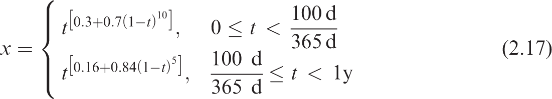
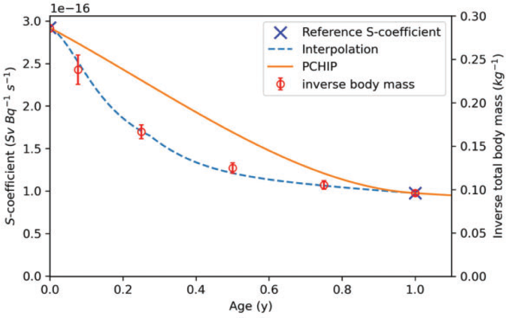
(35) Fig. 2.1 provides justification for the interpolation described in Eqs (2.16) and (2.17). Table 4.3 in Publication 89 (ICRP, 2002) provides the total body mass of European infants (Eveleth and Tanner, 1990; ICRP, 2002). The interpolated function is designed to provide a better fit for the variable growth patterns taking place within the first year of life.

Fig. 2.1.

S-coefficient interpolation within the first year. The crosses represent S-coefficients at ages 0 and 1 year for the emissions from tritiated water from ‘Other’ systemic tissue irradiating the muscle. The dashed line is the interpolated function provided in Eq. (2.16). The circles are plotted against the right-hand y-axis and are the inverse of the total body mass provided in Eq. (4.3) of Publication 89 (ICRP, 2002). The piecewise cubic Hermite spline (PCHIP) curve is the result if a PCHIP interpolation was applied between birth and 1 year of age.

2.2.1. Other uses of reference SAFs

(36) The SAFs in this publication have been computed for the primary purpose of computing organ equivalent dose and effective dose coefficients for use in radiation protection. However, these SAFs are likely to be useful for a variety of additional internal dosimetry applications, including nuclear medicine (studied by ICRP Task Group 36) and internal dose reconstruction. Users of these SAFs are advised to keep in mind that they are consistent with the reference individuals defined in Section 3. Care should therefore be taken when applying them to non-reference individuals. Use of these SAFs should be made with an understanding that one is treating at least one component of the internal dosimetry calculation (fraction of emitted energy absorbed per unit mass) as equivalent to that in the ICRP reference individuals.

3. ICRP Reference Individuals

(37) The reference individuals are idealised persons used for the calculation of effective dose (ICRP, 2007). The parameters defining the reference individuals include anatomical and physiological parameters. The physiological parameters inform the biokinetic modelling of activity, while the anatomical parameters form the basis for computational phantoms and models used to compute SAFs. While the calculation can be thought of in terms of the product of a source (or biokinetic) term and an energy absorption term, the two terms should be computed in a manner consistent with one another. The characterisation and definition of the reference individuals serve as a guiding mechanism for ensuring that the two terms involved in the calculation of internal doses maintain consistency with one another. The reference SAFs provided in this publication are therefore reference values, consistent with the reference individual definition.

3.1. Sources of reference mass data

3.1.1. Publication 89

(38) Publication 89 (ICRP, 2002) provides most of the reference masses of the reference individuals for males and females of six ages (newborn, 1 year, 5 years, 10 years, 15 years, and adult). In addition to publishing reference masses based on research in the literature, Publication 89 included reference values published previously in Publication 66 (ICRP, 1994) on the respiratory tract, Publication 70 (ICRP, 1995a) on the skeleton, Publication 88 (ICRP, 2001) on the embryo/fetus, and Publication 23 (ICRP, 1975) on the definition of Reference Man.

(39) Table 2.8 in Publication 89 (ICRP, 2002) provides a summary table of reference masses of organs and tissues by sex and age. For almost all organs and tissues listed in Table 2.8, the listed mass values do not include the blood perfusing that organ or tissue (i.e. organ parenchyma mass alone). Often, radioactive material will be taken up in tissue in proportion to the parenchyma tissue mass, so it is generally desirable to describe source masses as exclusive of blood. However, as the energy absorption takes place in the entire mass of an organ or tissue which contains blood, the target mass needs to include the mass of blood perfusing the tissue.

(40) Table 2.14 in Publication 89 (ICRP, 2002) provides a reference blood distribution for the adult male and female, but does not contain similar information for the younger reference ages. Table 2.14 gives the percentage of the total body blood volume which is found in each of the organs or tissues listed.

3.1.2. Publication 66

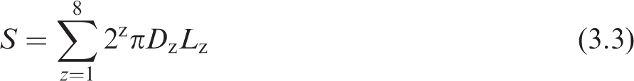
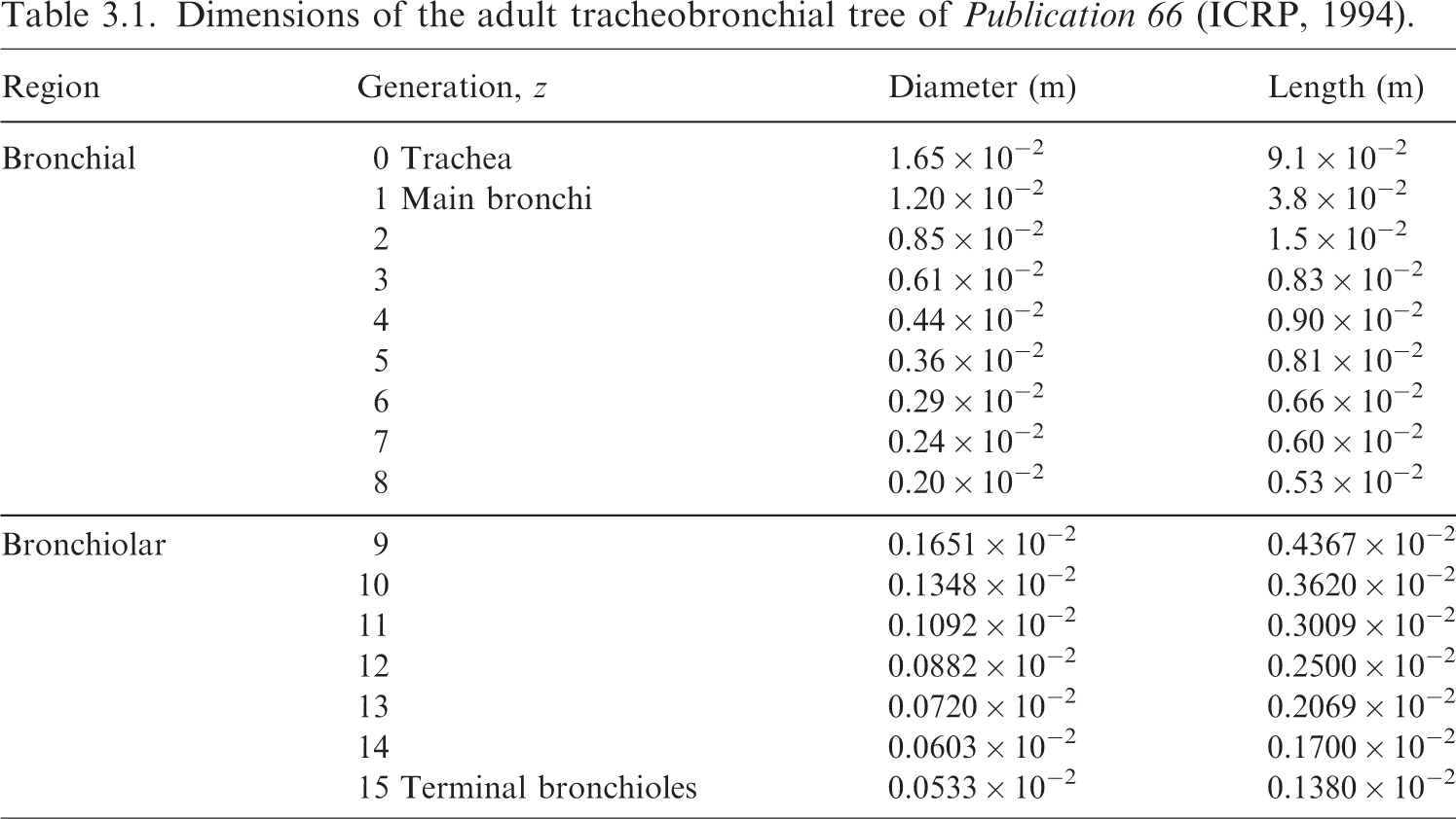
(41) Publication 66 (ICRP, 1994) provides detailed information on the HRTM. Table 5 in Publication 66 was reprinted as Table 5.3 in Publication 89 (ICRP, 2002), and provides reference masses of epithelial target tissues in the respiratory tract, as well as masses for the ET and TH lymph nodes.

(42) Table 5 of Publication 66 (ICRP, 1994) did not provide masses for the newborn, but newborn masses were provided in Table 5.3 of Publication 89 (ICRP, 2002). During the preparation of the EIR series of publications, it became clear that the reference newborn masses for the bronchi and bronchiole source and target regions were not computed in Publications 71 (ICRP, 1995b) and 89 in a manner consistent with the methods of Publication 66. In this work, new reference masses are provided for the newborn bronchi and bronchiole regions. Note that considerable uncertainty exists in the applicability of Publication 66 methodology for the newborn. Nevertheless, it is desirable to proceed with a method consistent with that used at other reference ages.

(43) The newborn masses are computed here in a method consistent with the method described in Publication 66 (ICRP, 1994). Fig. 2 in Publication 66 depicts the stylised cylindrical dosimetry model for the airway regions. The mass of a tissue layer beginning at some depth d₁ through a depth d₂ could be computed as given in Eq. (3.1), where D is the diameter and L is the length of the cylindrical airway, and $\rho$ is the mass density of the tissue (taken as 1.00 g cm⁻³ in Publication 66):

$${\mathit{\text{m}}}_{\text{r}}=\rho L\pi \left[{\left(\frac{D}{2}+d_2\right)}^2-{\left(\frac{D}{2}+d_1\right)}^2\right]$$

(3.1)

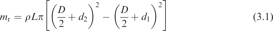
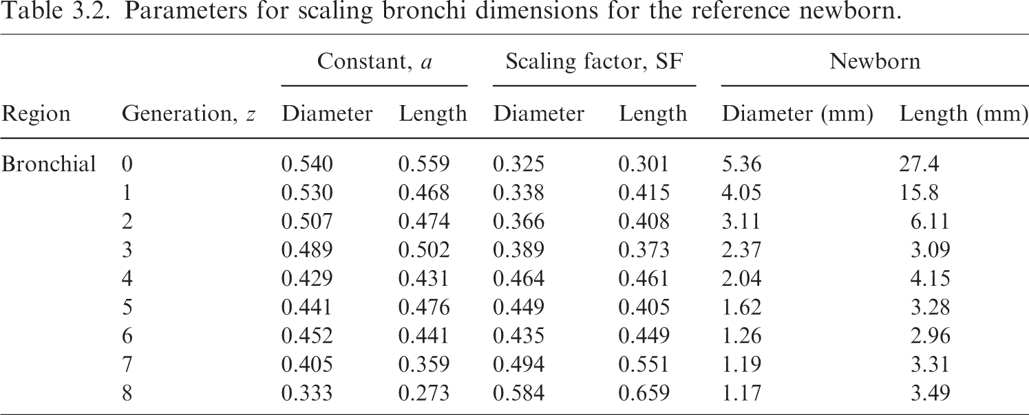
As the depths and thicknesses of the tissue layers are small compared with the airway diameter, the mass can be more simply approximated as the product of mass density, the surface area of the airway, $S$ , and the thickness of the layer of interest, $d$ :

$$m_{\text{r}}\cong \rho Sd=\rho S\left(d_2-d_1\right)$$

(3.2)

• (44) The airway surface area is computed using the dimensional model of the tracheobronchial tree provided in Publication 66 (ICRP, 1994) and repeated here in Table 3.1. The surface area of the bronchial region is given by summing the relative contributions of each branch (1 through 8) in the bronchial tree as shown in Eq. (3.3), where $z$ is the generation of the branch, and $D_{\mathrm{z}}$ and $L_{\text{z}}$ are the diameter and length of the branch, respectively:

  $$S=\sum _{z=1}^8{2}^{\text{z}}\pi D_{\text{z}}{L}_{\text{z}}$$

  (3.3)

  Table 3.1.

  Dimensions of the adult tracheobronchial tree of Publication 66 (ICRP, 1994).

  

  Region	Generation, z	Diameter (m)	Length (m)
  Bronchial	0 Trachea	1.65 × 10−2	9.1 × 10−2
  	1 Main bronchi	1.20 × 10−2	3.8 × 10−2
  	2	0.85 × 10−2	1.5 × 10−2
  	3	0.61 × 10−2	0.83 × 10−2
  	4	0.44 × 10−2	0.90 × 10−2
  	5	0.36 × 10−2	0.81 × 10−2
  	6	0.29 × 10−2	0.66 × 10−2
  	7	0.24 × 10−2	0.60 × 10−2
  	8	0.20 × 10−2	0.53 × 10−2
  Bronchiolar	9	0.1651 × 10−2	0.4367 × 10−2
  	10	0.1348 × 10−2	0.3620 × 10−2
  	11	0.1092 × 10−2	0.3009 × 10−2
  	12	0.0882 × 10−2	0.2500 × 10−2
  	13	0.0720 × 10−2	0.2069 × 10−2
  	14	0.0603 × 10−2	0.1700 × 10−2
  	15 Terminal bronchioles	0.0533 × 10−2	0.1380 × 10−2

• (45) Publication 66 (ICRP, 1994) provides information on scaling the airway dimensions to account for differences in age and sex. For the bronchi region, Table 4 of Publication 66 provides instructions on scaling each generation 1–8 based on a study by Phalen et al. (1985). The footnote of that table provides an equation for a scaling factor ( $\mathrm{S}\mathrm{F}$ ) dependent on body height, $H$ , and a constant, $a$ . The SFs are reproduced here in Table 3.2 based on a reference height for the newborn of 0.51 m:

  $$\mathrm{S}\mathrm{F}=a\left(H-1.76\right)+1$$

  (3.4)

  Table 3.2.

  Parameters for scaling bronchi dimensions for the reference newborn.

  

  		Constant, $a$		Scaling factor, SF		Newborn
  Region	Generation, z	Diameter	Length	Diameter	Length	Diameter (mm)	Length (mm)
  Bronchial	0	0.540	0.559	0.325	0.301	5.36	27.4
  	1	0.530	0.468	0.338	0.415	4.05	15.8
  	2	0.507	0.474	0.366	0.408	3.11	6.11
  	3	0.489	0.502	0.389	0.373	2.37	3.09
  	4	0.429	0.431	0.464	0.461	2.04	4.15
  	5	0.441	0.476	0.449	0.405	1.62	3.28
  	6	0.452	0.441	0.435	0.449	1.26	2.96
  	7	0.405	0.359	0.494	0.551	1.19	3.31
  	8	0.333	0.273	0.584	0.659	1.17	3.49

• (46) Applying Eq. (3.4) with the newborn airway dimensions yields a surface area for the newborn bronchial region of 7.39 × 10⁻³ m². Table 3.3 summarises the computation of the newborn bronchi source and target regions.

  Table 3.3.

  Revised masses for newborn bronchi regions.

  

  Region	Inner depth, $d_1$ (µm)	Outer depth, $d_2$ (µm)	Thickness, $d$ (µm)	Mass (g)
  Bronch-bas	35	50	15	0.111
  Bronch-sec	10	40	30	0.222
  Bronchi-b	0	60	60	0.443
  Bronchi-q	60	70	10	0.0740

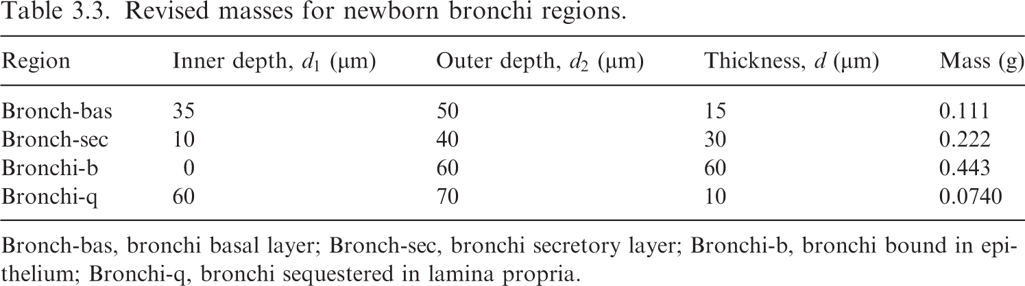
  Bronch-bas, bronchi basal layer; Bronch-sec, bronchi secretory layer; Bronchi-b, bronchi bound in epithelium; Bronchi-q, bronchi sequestered in lamina propria.

• (47) A similar calculation is performed to determine the masses of the bronchiolar regions in the newborn. Eq. (3.3) can be applied to scaled dimensions for generations 9–15. Publication 66 (ICRP, 1994) provides the following description for scaling the bronchiole diameter and length:

The diameter of the bronchioles (generations 9–15) is obtained by interpolating between the reference diameter of the last generation of bronchi (generation 8) and the first generation of respiratory bronchioles (generation 16). The unique parabola, which has its minimum at the diameter of the 16 ^th airway generation, provides a good fit to the bronchiolar airway diameters measured by Phalen et al. (1985) for adult subjects. This parabolic interpolation is assumed to apply to younger subjects also. In a similar manner, the lengths of the bronchioles (generations 9–15) are obtained by hyperbolic interpolation between the reference lengths of airways in the 8 ^th and 16 ^th generations.

(48) The parabolic interpolation for the diameters is applied as given in Eq. (3.5), while the hyperbolic interpolation for the lengths in each generation is given in Eq. (3.6):

$$D_{\text{z}}=D_{16}+\left(D_8-D_{16}\right)\frac{{\left(z-16\right)}^2}{{\left(8-16\right)}^2}$$

(3.5)

$$L_{\text{z}}=L_{16}+\left(L_8-L_{16}\right)\left(\frac{16}{z}-1\right)$$

(3.6)

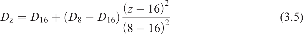
In order to apply the above equations, the newborn diameters and lengths for generations 8 and 16 must be determined. The values for generation 8 were determined previously (see Table 3.2). For generation 16, Publication 66 (ICRP, 1994) describes scaling by the one-third power of the functional residual capacity (FRC). However, Publication 66 only provides FRC values down to an age of 3 months. Gaultier et al. (1979) provides an equation [Eq. (3.7)] for FRC for children from birth to 3 years of age:

$$\mathrm{F}\mathrm{R}{\mathrm{C}}_{\text{male}} \left(\mathrm{m}\mathrm{L}\right)=-269+6.9H \left(\mathrm{c}\mathrm{m}\right)$$

$$\mathrm{F}\mathrm{R}{\mathrm{C}}_{\text{female}} \left(\mathrm{m}\mathrm{L}\right)=-204+5.92H \left(\mathrm{c}\mathrm{m}\right)$$

(3.7)

Using the newborn reference height of 0.51 m gives a sex averaged FRC of 90 mL. Eq. (3.8) applies the cube root scaling to determine the diameter and length (designated as X_16,newborn) for generation 16:

$$X_{16\text{,newborn}}=X_{16,\text{adult}}{\left(\frac{\mathrm{F}\mathrm{R}{\mathrm{C}}_{\text{newborn}}}{\mathrm{F}\mathrm{R}{\mathrm{C}}_{\text{adult}}}\right)}^{1/3}$$

$$D_{16\text{,newborn}}=1.535\times {10}^{-4} \mathrm{m}$$

$$L_{16\text{,newborn}}=3.311\times {10}^{-4} \mathrm{m}$$

(3.8)

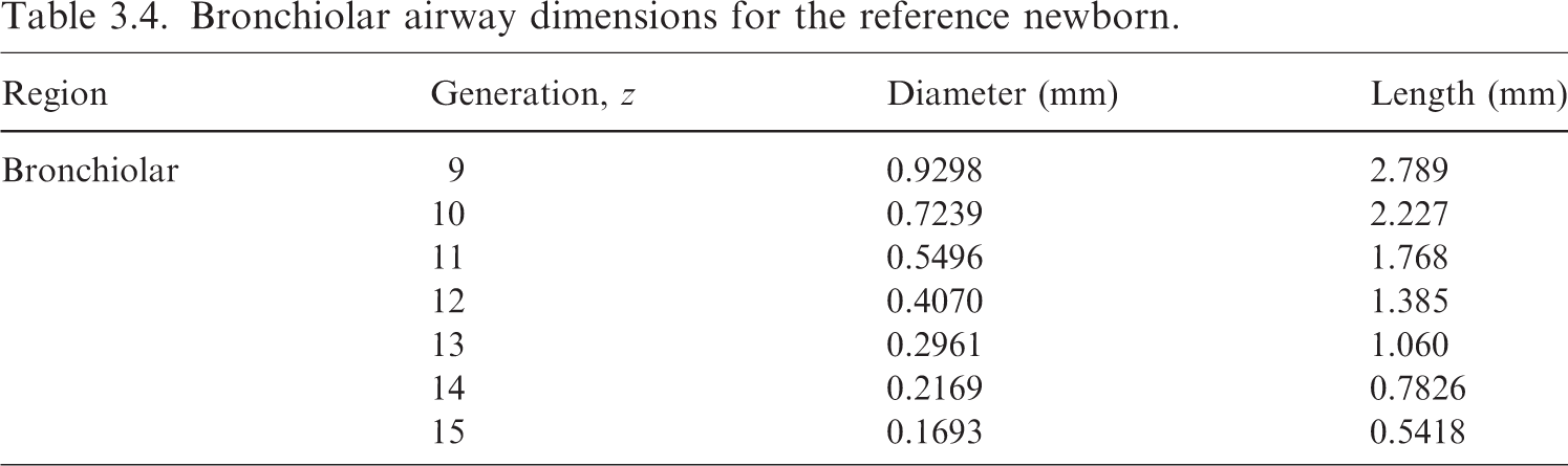
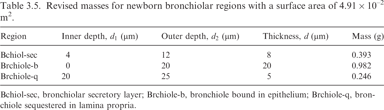
• (49) Eqs (3.5) and (3.6) can now be applied to determine the newborn airway dimensions for generations 9–15 given in Table 3.4. Eq. (3.3) is then adapted to the bronchiolar generations to give a newborn bronchiole surface area of 4.91 × 10⁻² m². The masses of the newborn bronchiole source and target regions are computed via Eq. (3.2), and are provided in Table 3.5.

Table 3.4.

Bronchiolar airway dimensions for the reference newborn.

Region	Generation, z	Diameter (mm)	Length (mm)
Bronchiolar	9	0.9298	2.789
	10	0.7239	2.227
	11	0.5496	1.768
	12	0.4070	1.385
	13	0.2961	1.060
	14	0.2169	0.7826
	15	0.1693	0.5418

Table 3.5.

Revised masses for newborn bronchiolar regions with a surface area of 4.91 × 10^–2 m².

Region	Inner depth, $d_1$ (µm)	Outer depth, $d_2$ (µm)	Thickness, $d$ (µm)	Mass (g)
Bchiol-sec	4	12	8	0.393
Brchiole-b	0	20	20	0.982
Brchiole-q	20	25	5	0.246

Bchiol-sec, bronchiolar secretory layer; Brchiole-b, bronchiole bound in epithelium; Brchiole-q, bronchiole sequestered in lamina propria.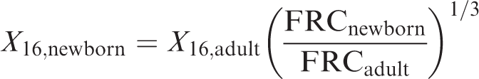

3.1.3. Publication 100

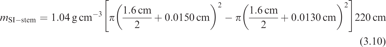
(50) Publication 100 (ICRP, 2006) provides detailed information on the HATM. While Publication 100 does not tabulate masses for the alimentary tract target tissues, Section 7 of that publication provides reference geometrical information about the size of the different alimentary tract regions. This information is used to compute reference masses for the alimentary tract target tissues.

(51) For example, Table 7.4 of Publication 100 (ICRP, 2006) provides reference lengths, and Table 7.5 of Publication 100 provides internal diameters for the small intestine. From the accompanying text, the target is assumed to be a continuous layer at 130–150 µm from the inner surface, and is independent of age and sex. Modelling the small intestine as a cylinder means the mass of the target layer can be computed as:

$$m_{\mathrm{S}\mathrm{I}-\mathrm{s}\mathrm{t}\mathrm{e}\mathrm{m}}={\rho }_{\text{tissue}}\left[\pi {\left(\frac{d}{2}+\mathrm{d}\mathrm{e}\mathrm{p}\mathrm{t}{\mathrm{h}}_{\text{outer}}\right)}^2-\pi {\left(\frac{d}{2}+\mathrm{d}\mathrm{e}\mathrm{p}\mathrm{t}{\mathrm{h}}_{\text{inner}}\right)}^2\right]l_{\text{cylinder}}$$

(3.9)

where ${\rho }_{\text{tissue}}$ is the mass density of tissue, $d$ is the internal diameter, $l_{\text{cylinder}}$ is the length of the small intestine, and $\mathrm{d}\mathrm{e}\mathrm{p}\mathrm{t}{\mathrm{h}}_{\text{outer}}$ and $\mathrm{d}\mathrm{e}\mathrm{p}\mathrm{t}{\mathrm{h}}_{\text{inner}}$ are the outer and inner boundaries of the target layer, respectively For the reference 10-year-old, the mass is computed as:

$$m_{\mathrm{S}\mathrm{I}-\mathrm{s}\mathrm{t}\mathrm{e}\mathrm{m}}=1.04\hspace{0.17em}{\mathrm{g}\hspace{0.17em}\mathrm{c}\mathrm{m}}^{-3}\left[\pi {\left(\frac{1.6\hspace{0.17em}\mathrm{c}\mathrm{m}}{2}+0.0150\hspace{0.17em}\mathrm{c}\mathrm{m}\right)}^2-\pi {\left(\frac{1.6\hspace{0.17em}\mathrm{c}\mathrm{m}}{2}+0.0130\hspace{0.17em}\mathrm{c}\mathrm{m}\right)}^2\right]220\hspace{0.17em}\mathrm{c}\mathrm{m}$$

(3.10)

$$m_{\mathrm{S}\mathrm{I}-\mathrm{s}\mathrm{t}\mathrm{e}\mathrm{m}}=2.34 \mathrm{g}$$

(3.11)

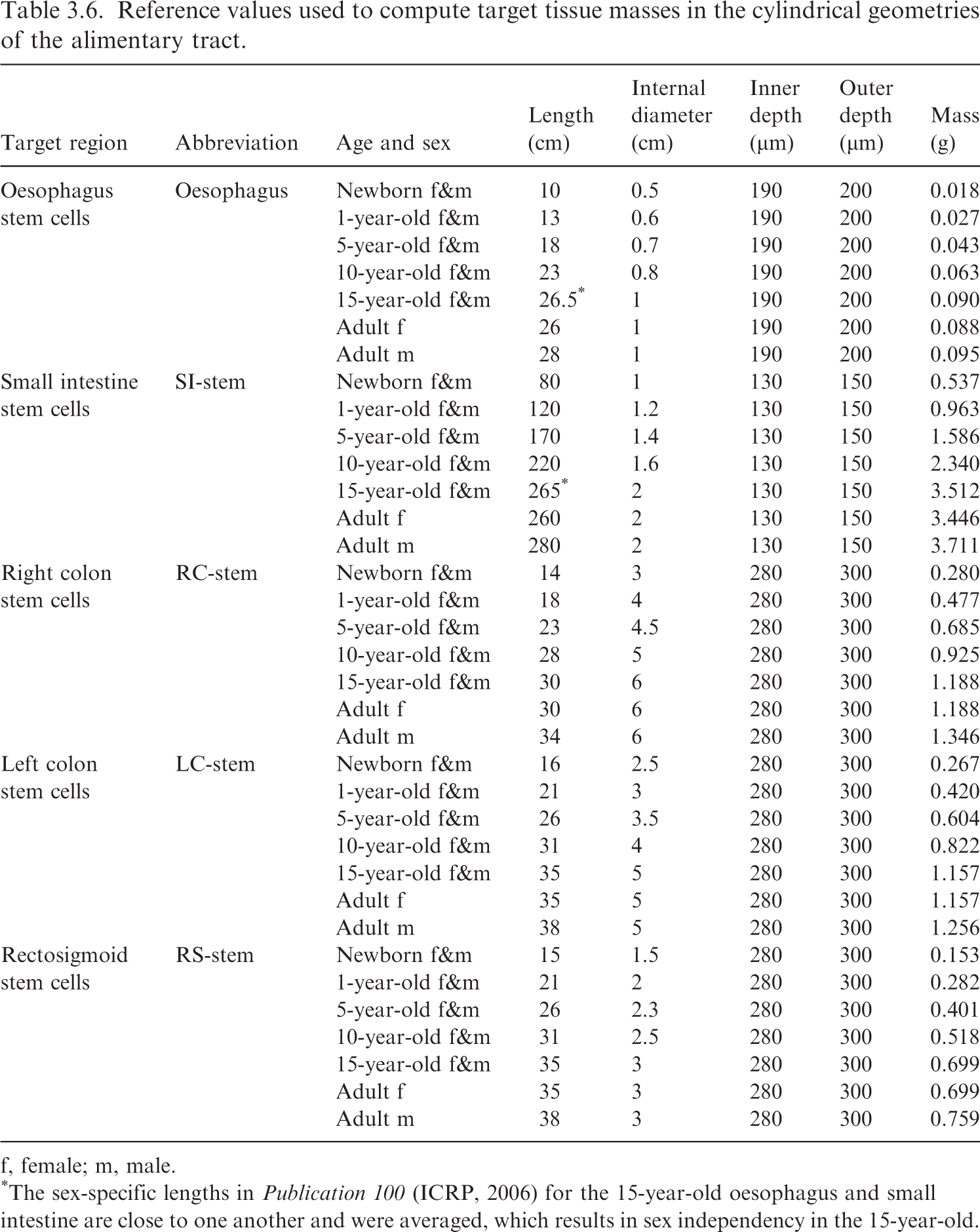
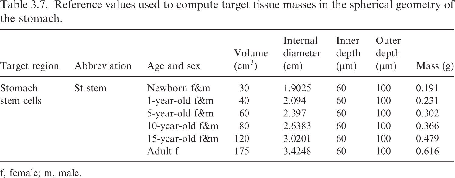
• (52) Table 3.6 summarises the reference information provided in Publication 100 (ICRP, 2006), and the resulting masses for the target tissues modelled as cylinders (oesophagus, small intestine, and colon). Table 3.7 contains the information for the stomach, which is modelled as a sphere.

Table 3.6.

Reference values used to compute target tissue masses in the cylindrical geometries of the alimentary tract.

Target region	Abbreviation	Age and sex	Length(cm)	Internal diameter (cm)	Inner depth (µm)	Outer depth (µm)	Mass (g)
Oesophagus stem cells	Oesophagus	Newborn f&m	10	0.5	190	200	0.018
		1-year-old f&m	13	0.6	190	200	0.027
		5-year-old f&m	18	0.7	190	200	0.043
		10-year-old f&m	23	0.8	190	200	0.063
		15-year-old f&m	26.5*	1	190	200	0.090
		Adult f	26	1	190	200	0.088
		Adult m	28	1	190	200	0.095
Small intestine stem cells	SI-stem	Newborn f&m	80	1	130	150	0.537
		1-year-old f&m	120	1.2	130	150	0.963
		5-year-old f&m	170	1.4	130	150	1.586
		10-year-old f&m	220	1.6	130	150	2.340
		15-year-old f&m	265*	2	130	150	3.512
		Adult f	260	2	130	150	3.446
		Adult m	280	2	130	150	3.711
Right colon stem cells	RC-stem	Newborn f&m	14	3	280	300	0.280
		1-year-old f&m	18	4	280	300	0.477
		5-year-old f&m	23	4.5	280	300	0.685
		10-year-old f&m	28	5	280	300	0.925
		15-year-old f&m	30	6	280	300	1.188
		Adult f	30	6	280	300	1.188
		Adult m	34	6	280	300	1.346
Left colon stem cells	LC-stem	Newborn f&m	16	2.5	280	300	0.267
		1-year-old f&m	21	3	280	300	0.420
		5-year-old f&m	26	3.5	280	300	0.604
		10-year-old f&m	31	4	280	300	0.822
		15-year-old f&m	35	5	280	300	1.157
		Adult f	35	5	280	300	1.157
		Adult m	38	5	280	300	1.256
Rectosigmoid stem cells	RS-stem	Newborn f&m	15	1.5	280	300	0.153
		1-year-old f&m	21	2	280	300	0.282
		5-year-old f&m	26	2.3	280	300	0.401
		10-year-old f&m	31	2.5	280	300	0.518
		15-year-old f&m	35	3	280	300	0.699
		Adult f	35	3	280	300	0.699
		Adult m	38	3	280	300	0.759

f, female; m, male.

^*The sex-specific lengths in Publication 100 (ICRP, 2006) for the 15-year-old oesophagus and small intestine are close to one another and were averaged, which results in sex independency in the 15-year-old.

Table 3.7.

Reference values used to compute target tissue masses in the spherical geometry of the stomach.

Target region	Abbreviation	Age and sex	Volume (cm3)	Internal diameter (cm)	Inner depth (µm)	Outer depth (µm)	Mass (g)
Stomach stem cells	St-stem	Newborn f&m	30	1.9025	60	100	0.191
		1-year-old f&m	40	2.094	60	100	0.231
		5-year-old f&m	60	2.397	60	100	0.302
		10-year-old f&m	80	2.6383	60	100	0.366
		15-year-old f&m	120	3.0201	60	100	0.479
		Adult f	175	3.4248	60	100	0.616

f, female; m, male.

3.2. Inclusion of blood and blood distribution model

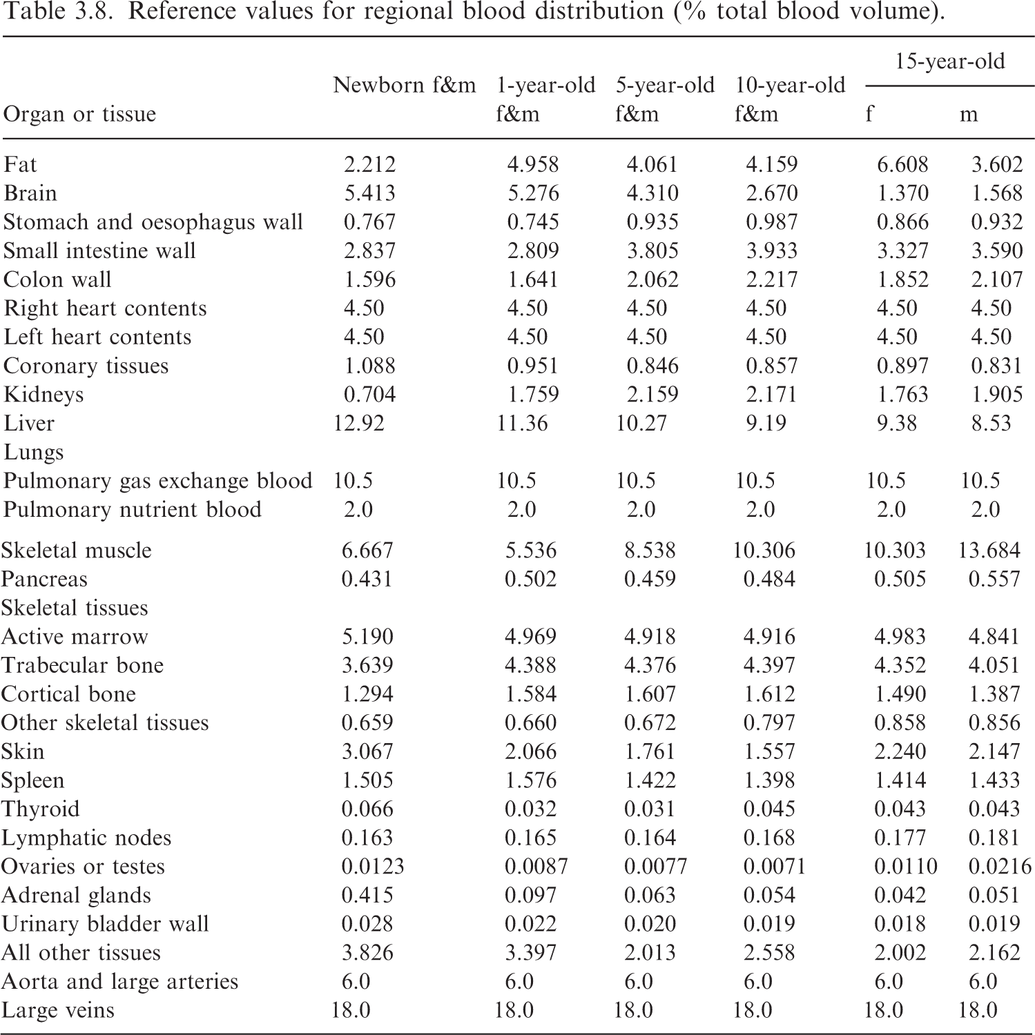
(53) The mass for most target regions requires the addition of blood to the masses listed in Table 2.8 of Publication 89 (ICRP, 2002). While Table 2.14 of Publication 89 provides the blood distribution for the reference adults, the publication does not explicitly report a blood distribution model for younger ages. Such blood distributions are provided in Wayson et al. (2018).

(54) The values in Table 6 of Wayson et al. (2018) are rounded for publication purposes. As they represent an intermediate step in the target mass calculation, unrounded values are used to compute the blood contribution to target masses (using a density of blood of 1.06 g cm^–3.) Table 3.8 provides the unrounded blood distribution values used in this publication to compute reference target masses inclusive of blood.

Table 3.8.

Reference values for regional blood distribution (% total blood volume).

Organ or tissue	Newborn f&m	1-year-old	5-year-old	10-year-old	15-year-old
		f&m	f&m	f&m	f	m
Fat	2.212	4.958	4.061	4.159	6.608	3.602
Brain	5.413	5.276	4.310	2.670	1.370	1.568
Stomach and oesophagus wall	0.767	0.745	0.935	0.987	0.866	0.932
Small intestine wall	2.837	2.809	3.805	3.933	3.327	3.590
Colon wall	1.596	1.641	2.062	2.217	1.852	2.107
Right heart contents	4.50	4.50	4.50	4.50	4.50	4.50
Left heart contents	4.50	4.50	4.50	4.50	4.50	4.50
Coronary tissues	1.088	0.951	0.846	0.857	0.897	0.831
Kidneys	0.704	1.759	2.159	2.171	1.763	1.905
Liver	12.92	11.36	10.27	9.19	9.38	8.53
Lungs
Pulmonary gas exchange blood	10.5	10.5	10.5	10.5	10.5	10.5
Pulmonary nutrient blood	2.0	2.0	2.0	2.0	2.0	2.0
Skeletal muscle	6.667	5.536	8.538	10.306	10.303	13.684
Pancreas	0.431	0.502	0.459	0.484	0.505	0.557
Skeletal tissues
Active marrow	5.190	4.969	4.918	4.916	4.983	4.841
Trabecular bone	3.639	4.388	4.376	4.397	4.352	4.051
Cortical bone	1.294	1.584	1.607	1.612	1.490	1.387
Other skeletal tissues	0.659	0.660	0.672	0.797	0.858	0.856
Skin	3.067	2.066	1.761	1.557	2.240	2.147
Spleen	1.505	1.576	1.422	1.398	1.414	1.433
Thyroid	0.066	0.032	0.031	0.045	0.043	0.043
Lymphatic nodes	0.163	0.165	0.164	0.168	0.177	0.181
Ovaries or testes	0.0123	0.0087	0.0077	0.0071	0.0110	0.0216
Adrenal glands	0.415	0.097	0.063	0.054	0.042	0.051
Urinary bladder wall	0.028	0.022	0.020	0.019	0.018	0.019
All other tissues	3.826	3.397	2.013	2.558	2.002	2.162
Aorta and large arteries	6.0	6.0	6.0	6.0	6.0	6.0
Large veins	18.0	18.0	18.0	18.0	18.0	18.0

f, female; m, male.

(55) For many target regions, the mass calculation is described in Eq. (3.12), where $f_{\text{blood}}$ is the fraction by volume of blood in the target region, $m_{\text{wb}}$ is the mass of blood in the body, and $m_{\text{Tparenchyma}}$ is the mass of the target region without blood:

$$m_{\text{T}}=f_{\text{blood}}{m}_{\text{wb}}+m_{\text{Tparenchyma}}$$

(3.12)

(56) As an example, the target mass of the spleen at 5 years of age is computed as:

$$m_{\text{spleen}}=\left(0.01422\right)\left(1500 \mathrm{g}\right)+50 \mathrm{g}=71.33 \mathrm{g}$$

(3.13)

(57) For regions in Table 3.8 which comprise multiple targets, the blood is split by parenchyma mass fraction across those targets. For example, Table 3.8 has a single entry for the lymphatic nodes, but this blood is split across the ET, TH, and systemic lymph node targets by their respective mass fractions.

(58) In the lung regions, the 2.0% nutrient blood is split by mass fraction across the bronchi wall, the bronchiolar wall, and the alveolar-interstitium (AI). The pulmonary gas exchange blood (10.5%) is assigned in its entirety to the AI.

(59) There are several target regions not specified in Table 3.8. It becomes problematic to use the ‘All other tissues’ category to assign blood to these regions. First, the total list of target regions remaining does not completely comprise ‘All other tissues’. Even if reasonable attempts are made to determine how much tissue mass corresponds to ‘All other tissues’, practical problems arise such as generating sex-dependent blood mass in tissues for which sex dependency does not exist in the reference model.

(60) Instead, an approach was adopted which uses a ratio of blood to lean body mass in the whole body, and applies that to each desired target region not specified in Table 3.8. The method is summarised mathematically in Eq. (3.14):

$$m_{\mathrm{b}\mathrm{l}\mathrm{o}\mathrm{o}\mathrm{d}\mathrm{ }\mathrm{i}\mathrm{n}\mathrm{ }\mathrm{t}\mathrm{i}\mathrm{s}\mathrm{s}\mathrm{u}\mathrm{e}}={\left(m_{\text{blood}}:m_{\text{tissue}}\right)}_{\text{lean}}{m}_{\text{Tparenchyma}}$$

(3.14)

The ratio of blood to lean body mass is computed using information regarding blood distribution and lean tissue mass:

$$\left(m_{\text{blood}}:m_{\text{tissue}}\right){}_{\text{lean}}=\frac{m_{\text{blood,wb}}\left(1.00-f_{\text{blood,fat}}-f_{\text{blood,aorta}}-f_{\text{blood,veins}}\right)}{m_{\text{total body}}-m_{\text{fat}}}$$

(3.15)

In Eq. (3.15), $f_{\text{blood,fat}}$ , $f_{\text{blood,aorta}}$ , and $f_{\text{blood,veins}}$ are the blood volume fractions in the respective regions. The mass of the total body (Table 2.8) and the mass of fat (Section 4.3.3) each come from values in Publication 89 (ICRP, 2002). For example, the blood in the 15-year-old female breast is computed as:

$$m_{\mathrm{b}\mathrm{l}\mathrm{o}\mathrm{o}\mathrm{d},\mathrm{b}\mathrm{r}\mathrm{e}\mathrm{a}\mathrm{s}\mathrm{t}}=\left(\frac{3500 \mathrm{g} \left(1.00-0.06608-0.060-0.18\right)}{\mathrm{53,000} \mathrm{g}-\mathrm{14,000} \mathrm{g}}\right)250 \mathrm{g}=15.6 \mathrm{g}$$

(3.16)

3.3. Age-dependent reference masses

(61) The masses of the reference individuals are tabulated by target and source regions. The 43 target regions (41 regions in each sex) consist of those tissues which contribute to effective dose, along with a select set of tissues which may also be of interest for different applications. The 79 source regions are regions where biokinetic modelling may assign activity.

3.3.1. Target region masses

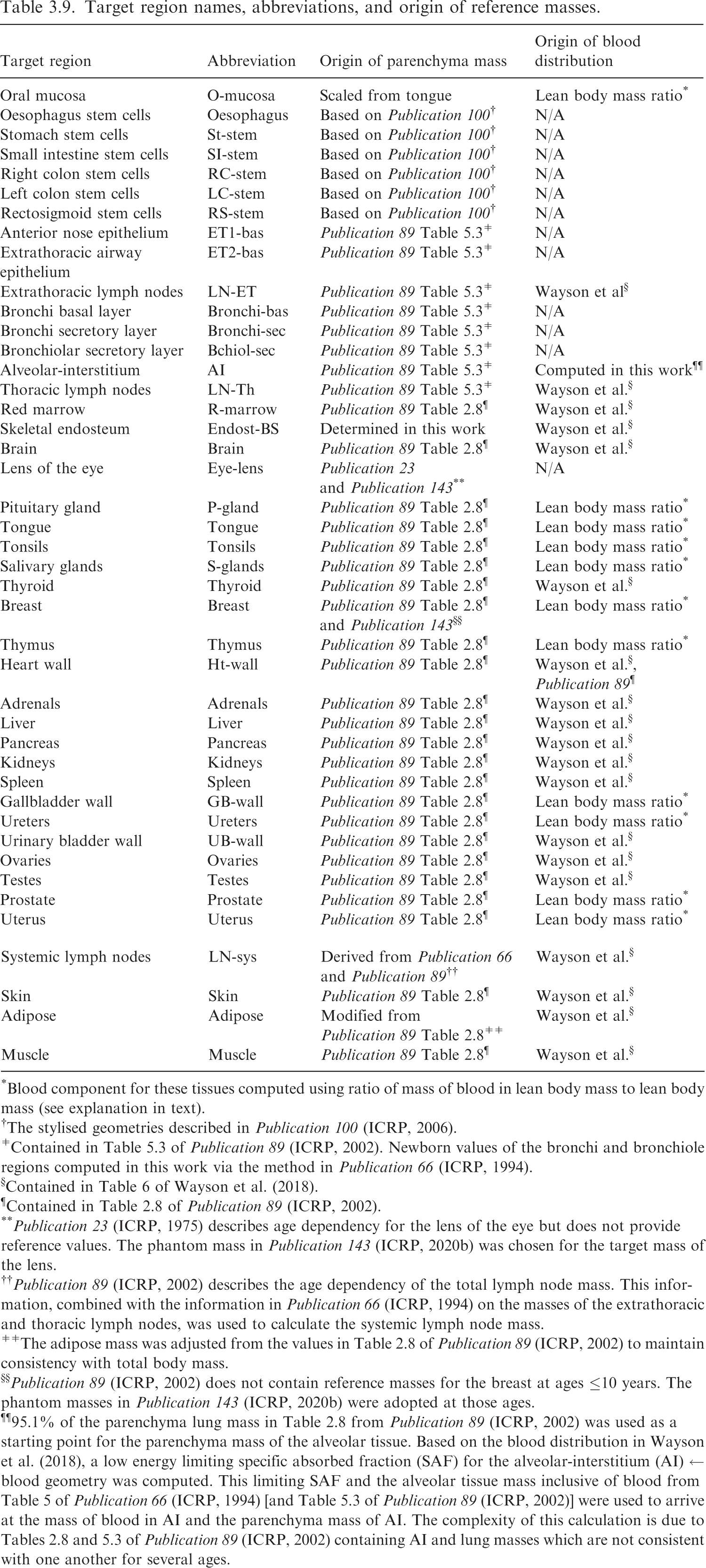
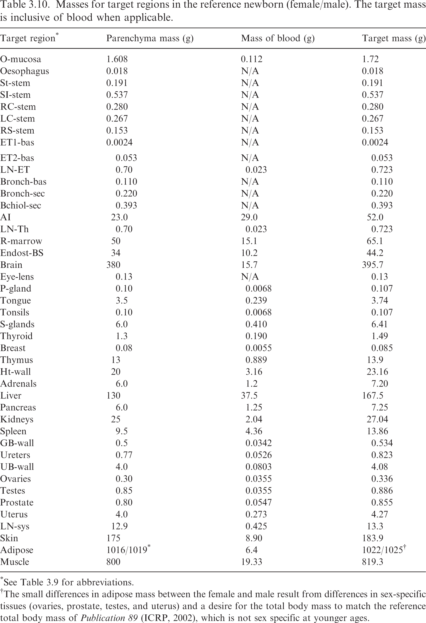
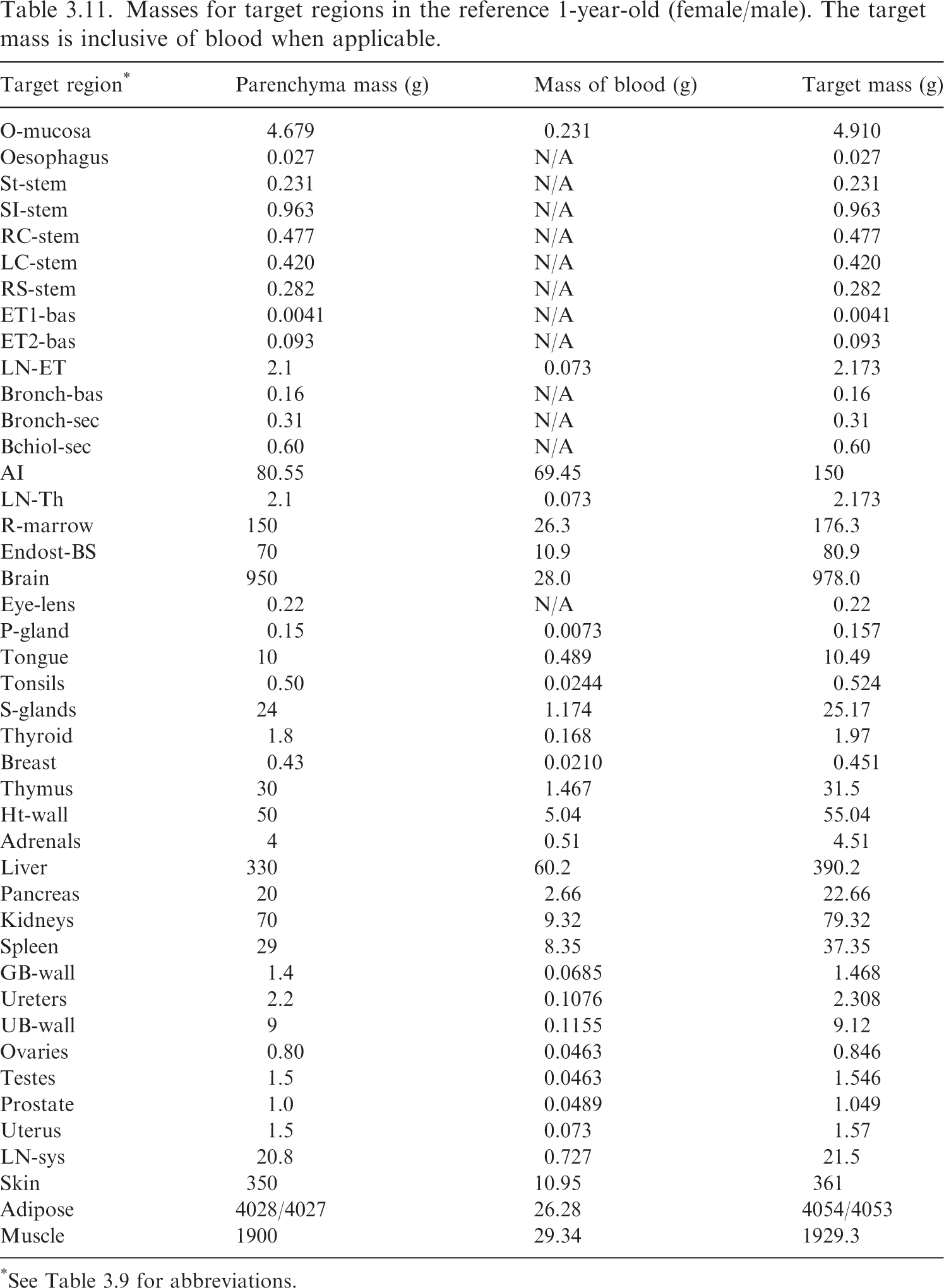
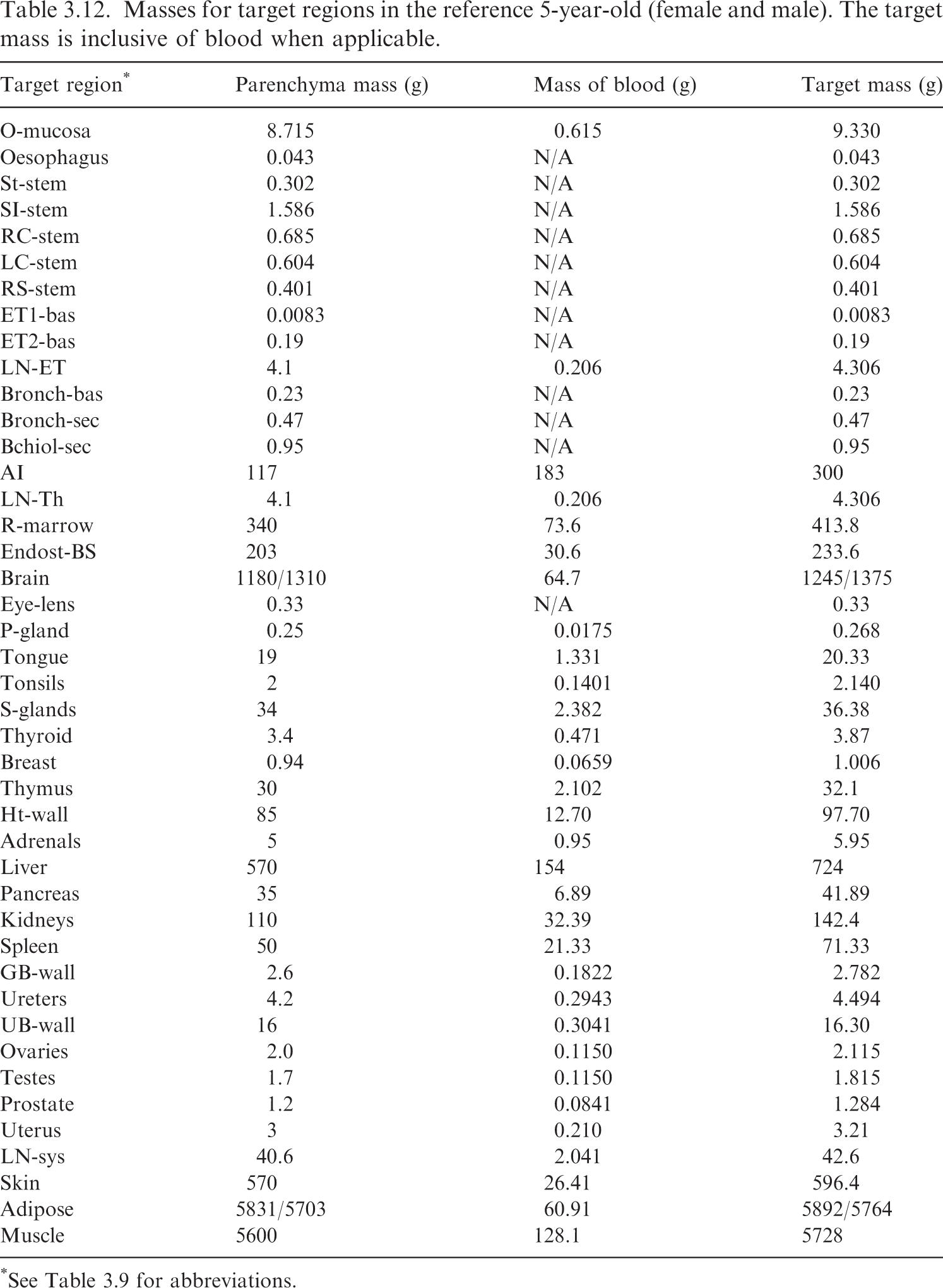
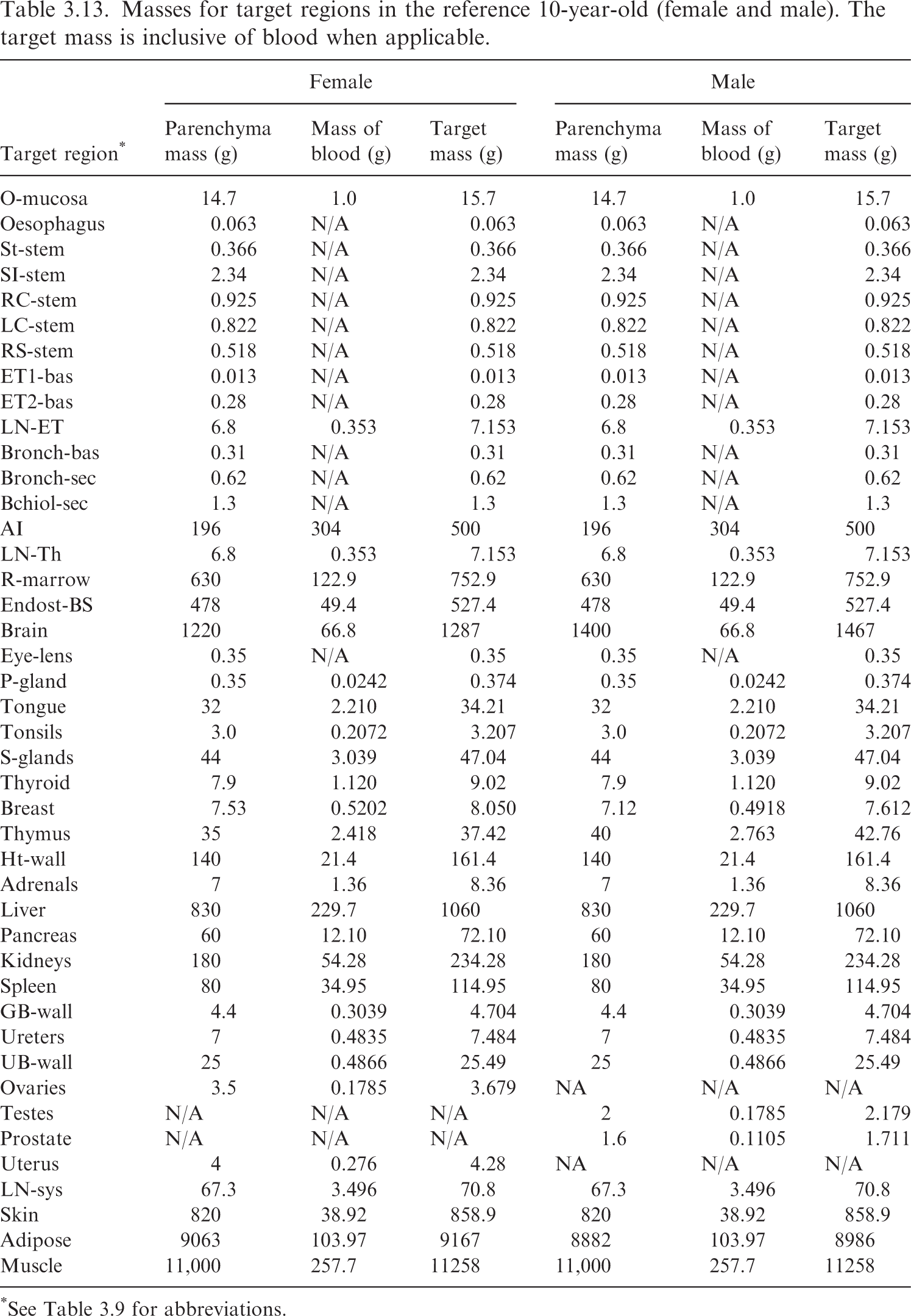
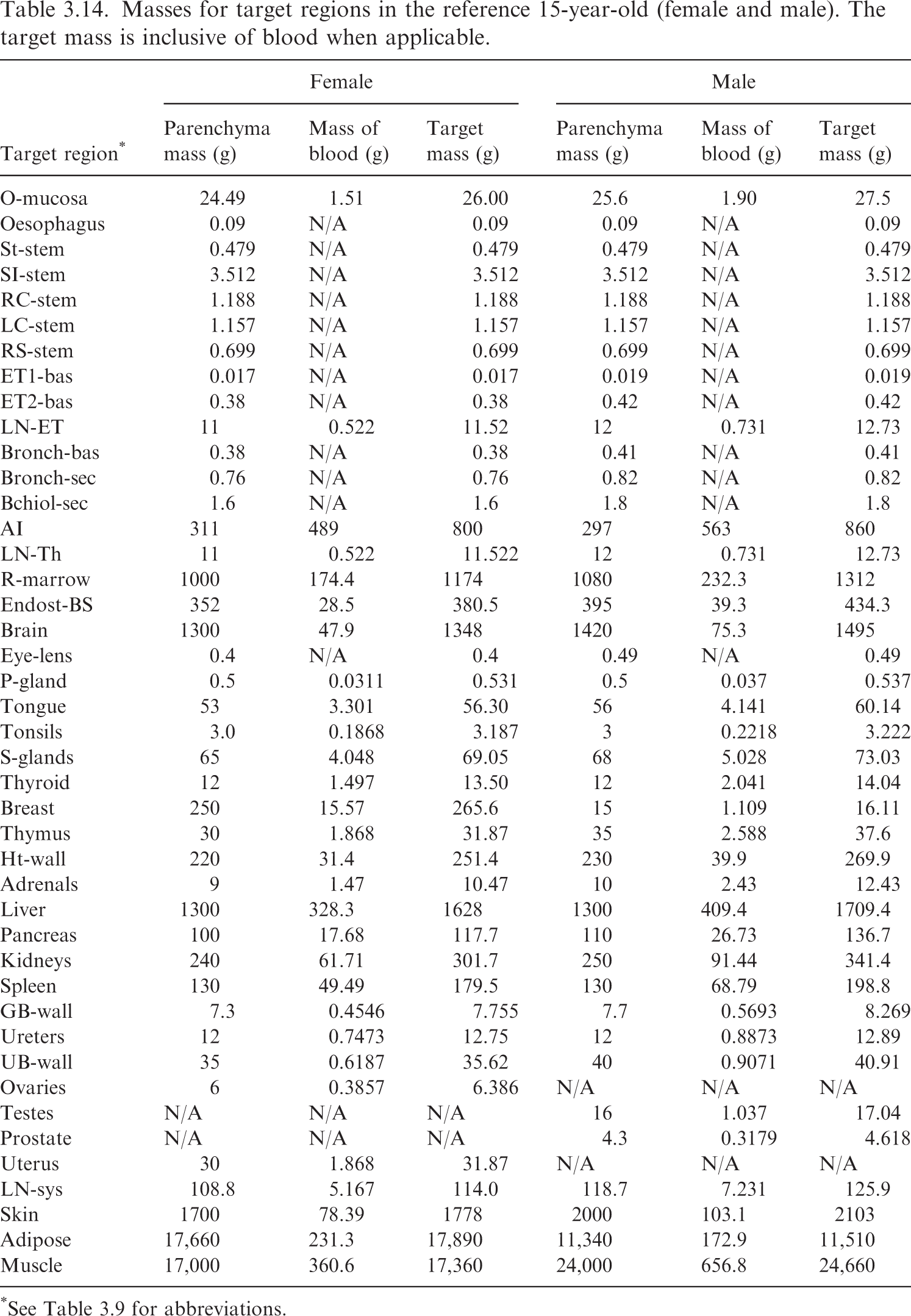
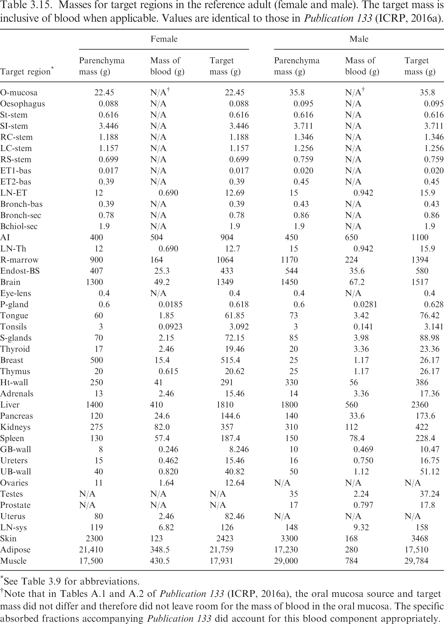
(62) Table 3.9 provides the list of target regions, their corresponding abbreviations, and information on the source and basis of the mass value. Tables 3.10–3.15 provide the reference masses for each of the reference individuals. When applicable, the contribution of blood to the mass of a target region is shown.

Table 3.9.

Target region names, abbreviations, and origin of reference masses.

Target region	Abbreviation	Origin of parenchyma mass	Origin of blood distribution
Oral mucosa	O-mucosa	Scaled from tongue	Lean body mass ratio*
Oesophagus stem cells	Oesophagus	Based on Publication 100 †	N/A
Stomach stem cells	St-stem	Based on Publication 100 †	N/A
Small intestine stem cells	SI-stem	Based on Publication 100 †	N/A
Right colon stem cells	RC-stem	Based on Publication 100 †	N/A
Left colon stem cells	LC-stem	Based on Publication 100 †	N/A
Rectosigmoid stem cells	RS-stem	Based on Publication 100 †	N/A
Anterior nose epithelium	ET1-bas	Publication 89 Table 5.3ǂ	N/A
Extrathoracic airway epithelium	ET2-bas	Publication 89 Table 5.3ǂ	N/A
Extrathoracic lymph nodes	LN-ET	Publication 89 Table 5.3ǂ	Wayson et al §
Bronchi basal layer	Bronchi-bas	Publication 89 Table 5.3ǂ	N/A
Bronchi secretory layer	Bronchi-sec	Publication 89 Table 5.3ǂ	N/A
Bronchiolar secretory layer	Bchiol-sec	Publication 89 Table 5.3ǂ	N/A
Alveolar-interstitium	AI	Publication 89 Table 5.3ǂ	Computed in this work ¶¶
Thoracic lymph nodes	LN-Th	Publication 89 Table 5.3ǂ	Wayson et al. §
Red marrow	R-marrow	Publication 89 Table 2.8¶	Wayson et al. §
Skeletal endosteum	Endost-BS	Determined in this work	Wayson et al. §
Brain	Brain	Publication 89 Table 2.8¶	Wayson et al. §
Lens of the eye	Eye-lens	Publication 23 and Publication 143**	N/A
Pituitary gland	P-gland	Publication 89 Table 2.8¶	Lean body mass ratio*
Tongue	Tongue	Publication 89 Table 2.8¶	Lean body mass ratio*
Tonsils	Tonsils	Publication 89 Table 2.8¶	Lean body mass ratio*
Salivary glands	S-glands	Publication 89 Table 2.8¶	Lean body mass ratio*
Thyroid	Thyroid	Publication 89 Table 2.8¶	Wayson et al. §
Breast	Breast	Publication 89 Table 2.8¶ and Publication 143§§	Lean body mass ratio*
Thymus	Thymus	Publication 89 Table 2.8¶	Lean body mass ratio*
Heart wall	Ht-wall	Publication 89 Table 2.8¶	Wayson et al. § , Publication 89 ¶
Adrenals	Adrenals	Publication 89 Table 2.8¶	Wayson et al. §
Liver	Liver	Publication 89 Table 2.8¶	Wayson et al. §
Pancreas	Pancreas	Publication 89 Table 2.8¶	Wayson et al. §
Kidneys	Kidneys	Publication 89 Table 2.8¶	Wayson et al. §
Spleen	Spleen	Publication 89 Table 2.8¶	Wayson et al. §
Gallbladder wall	GB-wall	Publication 89 Table 2.8¶	Lean body mass ratio*
Ureters	Ureters	Publication 89 Table 2.8¶	Lean body mass ratio*
Urinary bladder wall	UB-wall	Publication 89 Table 2.8¶	Wayson et al. §
Ovaries	Ovaries	Publication 89 Table 2.8¶	Wayson et al. §
Testes	Testes	Publication 89 Table 2.8¶	Wayson et al. §
Prostate	Prostate	Publication 89 Table 2.8¶	Lean body mass ratio*
Uterus	Uterus	Publication 89 Table 2.8¶	Lean body mass ratio*
Systemic lymph nodes	LN-sys	Derived from Publication 66 and Publication 89 ††	Wayson et al. §
Skin	Skin	Publication 89 Table 2.8¶	Wayson et al. §
Adipose	Adipose	Modified from Publication 89 Table 2.8ǂǂ	Wayson et al. §
Muscle	Muscle	Publication 89 Table 2.8¶	Wayson et al. §

^*Blood component for these tissues computed using ratio of mass of blood in lean body mass to lean body mass (see explanation in text).

^†The stylised geometries described in Publication 100 (ICRP, 2006).

^ǂContained in Table 5.3 of Publication 89 (ICRP, 2002). Newborn values of the bronchi and bronchiole regions computed in this work via the method in Publication 66 (ICRP, 1994).

^§Contained in Table 6 of Wayson et al. (2018).

^¶Contained in Table 2.8 of Publication 89 (ICRP, 2002).

^**Publication 23 (ICRP, 1975) describes age dependency for the lens of the eye but does not provide reference values. The phantom mass in Publication 143 (ICRP, 2020b) was chosen for the target mass of the lens.

^††Publication 89 (ICRP, 2002) describes the age dependency of the total lymph node mass. This information, combined with the information in Publication 66 (ICRP, 1994) on the masses of the extrathoracic and thoracic lymph nodes, was used to calculate the systemic lymph node mass.

^ǂǂThe adipose mass was adjusted from the values in Table 2.8 of Publication 89 (ICRP, 2002) to maintain consistency with total body mass.

^§§Publication 89 (ICRP, 2002) does not contain reference masses for the breast at ages ≤10 years. The phantom masses in Publication 143 (ICRP, 2020b) were adopted at those ages.

^¶¶95.1% of the parenchyma lung mass in Table 2.8 from Publication 89 (ICRP, 2002) was used as a starting point for the parenchyma mass of the alveolar tissue. Based on the blood distribution in Wayson et al. (2018), a low energy limiting specific absorbed fraction (SAF) for the alveolar-interstitium (AI) ← blood geometry was computed. This limiting SAF and the alveolar tissue mass inclusive of blood from Table 5 of Publication 66 (ICRP, 1994) [and Table 5.3 of Publication 89 (ICRP, 2002)] were used to arrive at the mass of blood in AI and the parenchyma mass of AI. The complexity of this calculation is due to Tables 2.8 and 5.3 of Publication 89 (ICRP, 2002) containing AI and lung masses which are not consistent with one another for several ages.

Table 3.10.

Masses for target regions in the reference newborn (female/male). The target mass is inclusive of blood when applicable.

Target region*	Parenchyma mass (g)	Mass of blood (g)	Target mass (g)
O-mucosa	1.608	0.112	1.72
Oesophagus	0.018	N/A	0.018
St-stem	0.191	N/A	0.191
SI-stem	0.537	N/A	0.537
RC-stem	0.280	N/A	0.280
LC-stem	0.267	N/A	0.267
RS-stem	0.153	N/A	0.153
ET1-bas	0.0024	N/A	0.0024
ET2-bas	0.053	N/A	0.053
LN-ET	0.70	0.023	0.723
Bronch-bas	0.110	N/A	0.110
Bronch-sec	0.220	N/A	0.220
Bchiol-sec	0.393	N/A	0.393
AI	23.0	29.0	52.0
LN-Th	0.70	0.023	0.723
R-marrow	50	15.1	65.1
Endost-BS	34	10.2	44.2
Brain	380	15.7	395.7
Eye-lens	0.13	N/A	0.13
P-gland	0.10	0.0068	0.107
Tongue	3.5	0.239	3.74
Tonsils	0.10	0.0068	0.107
S-glands	6.0	0.410	6.41
Thyroid	1.3	0.190	1.49
Breast	0.08	0.0055	0.085
Thymus	13	0.889	13.9
Ht-wall	20	3.16	23.16
Adrenals	6.0	1.2	7.20
Liver	130	37.5	167.5
Pancreas	6.0	1.25	7.25
Kidneys	25	2.04	27.04
Spleen	9.5	4.36	13.86
GB-wall	0.5	0.0342	0.534
Ureters	0.77	0.0526	0.823
UB-wall	4.0	0.0803	4.08
Ovaries	0.30	0.0355	0.336
Testes	0.85	0.0355	0.886
Prostate	0.80	0.0547	0.855
Uterus	4.0	0.273	4.27
LN-sys	12.9	0.425	13.3
Skin	175	8.90	183.9
Adipose	1016/1019*	6.4	1022/1025 †
Muscle	800	19.33	819.3

^*See Table 3.9 for abbreviations.

^†The small differences in adipose mass between the female and male result from differences in sex-specific tissues (ovaries, prostate, testes, and uterus) and a desire for the total body mass to match the reference total body mass of Publication 89 (ICRP, 2002), which is not sex specific at younger ages.

Table 3.11.

Masses for target regions in the reference 1-year-old (female/male). The target mass is inclusive of blood when applicable.

Target region*	Parenchyma mass (g)	Mass of blood (g)	Target mass (g)
O-mucosa	4.679	0.231	4.910
Oesophagus	0.027	N/A	0.027
St-stem	0.231	N/A	0.231
SI-stem	0.963	N/A	0.963
RC-stem	0.477	N/A	0.477
LC-stem	0.420	N/A	0.420
RS-stem	0.282	N/A	0.282
ET1-bas	0.0041	N/A	0.0041
ET2-bas	0.093	N/A	0.093
LN-ET	2.1	0.073	2.173
Bronch-bas	0.16	N/A	0.16
Bronch-sec	0.31	N/A	0.31
Bchiol-sec	0.60	N/A	0.60
AI	80.55	69.45	150
LN-Th	2.1	0.073	2.173
R-marrow	150	26.3	176.3
Endost-BS	70	10.9	80.9
Brain	950	28.0	978.0
Eye-lens	0.22	N/A	0.22
P-gland	0.15	0.0073	0.157
Tongue	10	0.489	10.49
Tonsils	0.50	0.0244	0.524
S-glands	24	1.174	25.17
Thyroid	1.8	0.168	1.97
Breast	0.43	0.0210	0.451
Thymus	30	1.467	31.5
Ht-wall	50	5.04	55.04
Adrenals	4	0.51	4.51
Liver	330	60.2	390.2
Pancreas	20	2.66	22.66
Kidneys	70	9.32	79.32
Spleen	29	8.35	37.35
GB-wall	1.4	0.0685	1.468
Ureters	2.2	0.1076	2.308
UB-wall	9	0.1155	9.12
Ovaries	0.80	0.0463	0.846
Testes	1.5	0.0463	1.546
Prostate	1.0	0.0489	1.049
Uterus	1.5	0.073	1.57
LN-sys	20.8	0.727	21.5
Skin	350	10.95	361
Adipose	4028/4027	26.28	4054/4053
Muscle	1900	29.34	1929.3

^*See Table 3.9 for abbreviations.

Table 3.12.

Masses for target regions in the reference 5-year-old (female and male). The target mass is inclusive of blood when applicable.

Target region*	Parenchyma mass (g)	Mass of blood (g)	Target mass (g)
O-mucosa	8.715	0.615	9.330
Oesophagus	0.043	N/A	0.043
St-stem	0.302	N/A	0.302
SI-stem	1.586	N/A	1.586
RC-stem	0.685	N/A	0.685
LC-stem	0.604	N/A	0.604
RS-stem	0.401	N/A	0.401
ET1-bas	0.0083	N/A	0.0083
ET2-bas	0.19	N/A	0.19
LN-ET	4.1	0.206	4.306
Bronch-bas	0.23	N/A	0.23
Bronch-sec	0.47	N/A	0.47
Bchiol-sec	0.95	N/A	0.95
AI	117	183	300
LN-Th	4.1	0.206	4.306
R-marrow	340	73.6	413.8
Endost-BS	203	30.6	233.6
Brain	1180/1310	64.7	1245/1375
Eye-lens	0.33	N/A	0.33
P-gland	0.25	0.0175	0.268
Tongue	19	1.331	20.33
Tonsils	2	0.1401	2.140
S-glands	34	2.382	36.38
Thyroid	3.4	0.471	3.87
Breast	0.94	0.0659	1.006
Thymus	30	2.102	32.1
Ht-wall	85	12.70	97.70
Adrenals	5	0.95	5.95
Liver	570	154	724
Pancreas	35	6.89	41.89
Kidneys	110	32.39	142.4
Spleen	50	21.33	71.33
GB-wall	2.6	0.1822	2.782
Ureters	4.2	0.2943	4.494
UB-wall	16	0.3041	16.30
Ovaries	2.0	0.1150	2.115
Testes	1.7	0.1150	1.815
Prostate	1.2	0.0841	1.284
Uterus	3	0.210	3.21
LN-sys	40.6	2.041	42.6
Skin	570	26.41	596.4
Adipose	5831/5703	60.91	5892/5764
Muscle	5600	128.1	5728

^*See Table 3.9 for abbreviations.

Table 3.13.

Masses for target regions in the reference 10-year-old (female and male). The target mass is inclusive of blood when applicable.

	Female			Male
Target region*	Parenchyma mass (g)	Mass of blood (g)	Target mass (g)	Parenchyma mass (g)	Mass of blood (g)	Target mass (g)
O-mucosa	14.7	1.0	15.7	14.7	1.0	15.7
Oesophagus	0.063	N/A	0.063	0.063	N/A	0.063
St-stem	0.366	N/A	0.366	0.366	N/A	0.366
SI-stem	2.34	N/A	2.34	2.34	N/A	2.34
RC-stem	0.925	N/A	0.925	0.925	N/A	0.925
LC-stem	0.822	N/A	0.822	0.822	N/A	0.822
RS-stem	0.518	N/A	0.518	0.518	N/A	0.518
ET1-bas	0.013	N/A	0.013	0.013	N/A	0.013
ET2-bas	0.28	N/A	0.28	0.28	N/A	0.28
LN-ET	6.8	0.353	7.153	6.8	0.353	7.153
Bronch-bas	0.31	N/A	0.31	0.31	N/A	0.31
Bronch-sec	0.62	N/A	0.62	0.62	N/A	0.62
Bchiol-sec	1.3	N/A	1.3	1.3	N/A	1.3
AI	196	304	500	196	304	500
LN-Th	6.8	0.353	7.153	6.8	0.353	7.153
R-marrow	630	122.9	752.9	630	122.9	752.9
Endost-BS	478	49.4	527.4	478	49.4	527.4
Brain	1220	66.8	1287	1400	66.8	1467
Eye-lens	0.35	N/A	0.35	0.35	N/A	0.35
P-gland	0.35	0.0242	0.374	0.35	0.0242	0.374
Tongue	32	2.210	34.21	32	2.210	34.21
Tonsils	3.0	0.2072	3.207	3.0	0.2072	3.207
S-glands	44	3.039	47.04	44	3.039	47.04
Thyroid	7.9	1.120	9.02	7.9	1.120	9.02
Breast	7.53	0.5202	8.050	7.12	0.4918	7.612
Thymus	35	2.418	37.42	40	2.763	42.76
Ht-wall	140	21.4	161.4	140	21.4	161.4
Adrenals	7	1.36	8.36	7	1.36	8.36
Liver	830	229.7	1060	830	229.7	1060
Pancreas	60	12.10	72.10	60	12.10	72.10
Kidneys	180	54.28	234.28	180	54.28	234.28
Spleen	80	34.95	114.95	80	34.95	114.95
GB-wall	4.4	0.3039	4.704	4.4	0.3039	4.704
Ureters	7	0.4835	7.484	7	0.4835	7.484
UB-wall	25	0.4866	25.49	25	0.4866	25.49
Ovaries	3.5	0.1785	3.679	NA	N/A	N/A
Testes	N/A	N/A	N/A	2	0.1785	2.179
Prostate	N/A	N/A	N/A	1.6	0.1105	1.711
Uterus	4	0.276	4.28	NA	N/A	N/A
LN-sys	67.3	3.496	70.8	67.3	3.496	70.8
Skin	820	38.92	858.9	820	38.92	858.9
Adipose	9063	103.97	9167	8882	103.97	8986
Muscle	11,000	257.7	11258	11,000	257.7	11258

^*See Table 3.9 for abbreviations.

Table 3.14.

Masses for target regions in the reference 15-year-old (female and male). The target mass is inclusive of blood when applicable.

	Female			Male
Target region*	Parenchyma mass (g)	Mass of blood (g)	Target mass (g)	Parenchyma mass (g)	Mass of blood (g)	Target mass (g)
O-mucosa	24.49	1.51	26.00	25.6	1.90	27.5
Oesophagus	0.09	N/A	0.09	0.09	N/A	0.09
St-stem	0.479	N/A	0.479	0.479	N/A	0.479
SI-stem	3.512	N/A	3.512	3.512	N/A	3.512
RC-stem	1.188	N/A	1.188	1.188	N/A	1.188
LC-stem	1.157	N/A	1.157	1.157	N/A	1.157
RS-stem	0.699	N/A	0.699	0.699	N/A	0.699
ET1-bas	0.017	N/A	0.017	0.019	N/A	0.019
ET2-bas	0.38	N/A	0.38	0.42	N/A	0.42
LN-ET	11	0.522	11.52	12	0.731	12.73
Bronch-bas	0.38	N/A	0.38	0.41	N/A	0.41
Bronch-sec	0.76	N/A	0.76	0.82	N/A	0.82
Bchiol-sec	1.6	N/A	1.6	1.8	N/A	1.8
AI	311	489	800	297	563	860
LN-Th	11	0.522	11.522	12	0.731	12.73
R-marrow	1000	174.4	1174	1080	232.3	1312
Endost-BS	352	28.5	380.5	395	39.3	434.3
Brain	1300	47.9	1348	1420	75.3	1495
Eye-lens	0.4	N/A	0.4	0.49	N/A	0.49
P-gland	0.5	0.0311	0.531	0.5	0.037	0.537
Tongue	53	3.301	56.30	56	4.141	60.14
Tonsils	3.0	0.1868	3.187	3	0.2218	3.222
S-glands	65	4.048	69.05	68	5.028	73.03
Thyroid	12	1.497	13.50	12	2.041	14.04
Breast	250	15.57	265.6	15	1.109	16.11
Thymus	30	1.868	31.87	35	2.588	37.6
Ht-wall	220	31.4	251.4	230	39.9	269.9
Adrenals	9	1.47	10.47	10	2.43	12.43
Liver	1300	328.3	1628	1300	409.4	1709.4
Pancreas	100	17.68	117.7	110	26.73	136.7
Kidneys	240	61.71	301.7	250	91.44	341.4
Spleen	130	49.49	179.5	130	68.79	198.8
GB-wall	7.3	0.4546	7.755	7.7	0.5693	8.269
Ureters	12	0.7473	12.75	12	0.8873	12.89
UB-wall	35	0.6187	35.62	40	0.9071	40.91
Ovaries	6	0.3857	6.386	N/A	N/A	N/A
Testes	N/A	N/A	N/A	16	1.037	17.04
Prostate	N/A	N/A	N/A	4.3	0.3179	4.618
Uterus	30	1.868	31.87	N/A	N/A	N/A
LN-sys	108.8	5.167	114.0	118.7	7.231	125.9
Skin	1700	78.39	1778	2000	103.1	2103
Adipose	17,660	231.3	17,890	11,340	172.9	11,510
Muscle	17,000	360.6	17,360	24,000	656.8	24,660

^*See Table 3.9 for abbreviations.

Table 3.15.

Masses for target regions in the reference adult (female and male). The target mass is inclusive of blood when applicable. Values are identical to those in Publication 133 (ICRP, 2016a).

	Female			Male
Target region*	Parenchyma mass (g)	Mass of blood (g)	Target mass (g)	Parenchyma mass (g)	Mass of blood (g)	Target mass (g)
O-mucosa	22.45	N/A †	22.45	35.8	N/A †	35.8
Oesophagus	0.088	N/A	0.088	0.095	N/A	0.095
St-stem	0.616	N/A	0.616	0.616	N/A	0.616
SI-stem	3.446	N/A	3.446	3.711	N/A	3.711
RC-stem	1.188	N/A	1.188	1.346	N/A	1.346
LC-stem	1.157	N/A	1.157	1.256	N/A	1.256
RS-stem	0.699	N/A	0.699	0.759	N/A	0.759
ET1-bas	0.017	N/A	0.017	0.020	N/A	0.020
ET2-bas	0.39	N/A	0.39	0.45	N/A	0.45
LN-ET	12	0.690	12.69	15	0.942	15.9
Bronch-bas	0.39	N/A	0.39	0.43	N/A	0.43
Bronch-sec	0.78	N/A	0.78	0.86	N/A	0.86
Bchiol-sec	1.9	N/A	1.9	1.9	N/A	1.9
AI	400	504	904	450	650	1100
LN-Th	12	0.690	12.7	15	0.942	15.9
R-marrow	900	164	1064	1170	224	1394
Endost-BS	407	25.3	433	544	35.6	580
Brain	1300	49.2	1349	1450	67.2	1517
Eye-lens	0.4	N/A	0.4	0.4	N/A	0.4
P-gland	0.6	0.0185	0.618	0.6	0.0281	0.628
Tongue	60	1.85	61.85	73	3.42	76.42
Tonsils	3	0.0923	3.092	3	0.141	3.141
S-glands	70	2.15	72.15	85	3.98	88.98
Thyroid	17	2.46	19.46	20	3.36	23.36
Breast	500	15.4	515.4	25	1.17	26.17
Thymus	20	0.615	20.62	25	1.17	26.17
Ht-wall	250	41	291	330	56	386
Adrenals	13	2.46	15.46	14	3.36	17.36
Liver	1400	410	1810	1800	560	2360
Pancreas	120	24.6	144.6	140	33.6	173.6
Kidneys	275	82.0	357	310	112	422
Spleen	130	57.4	187.4	150	78.4	228.4
GB-wall	8	0.246	8.246	10	0.469	10.47
Ureters	15	0.462	15.46	16	0.750	16.75
UB-wall	40	0.820	40.82	50	1.12	51.12
Ovaries	11	1.64	12.64	N/A	N/A	N/A
Testes	N/A	N/A	N/A	35	2.24	37.24
Prostate	N/A	N/A	N/A	17	0.797	17.8
Uterus	80	2.46	82.46	N/A	N/A	N/A
LN-sys	119	6.82	126	148	9.32	158
Skin	2300	123	2423	3300	168	3468
Adipose	21,410	348.5	21,759	17,230	280	17,510
Muscle	17,500	430.5	17,931	29,000	784	29,784

^*See Table 3.9 for abbreviations.

^†Note that in Tables A.1 and A.2 of Publication 133 (ICRP, 2016a), the oral mucosa source and target mass did not differ and therefore did not leave room for the mass of blood in the oral mucosa. The specific absorbed fractions accompanying Publication 133 did account for this blood component appropriately.

3.3.2. Source region masses (details and origin)

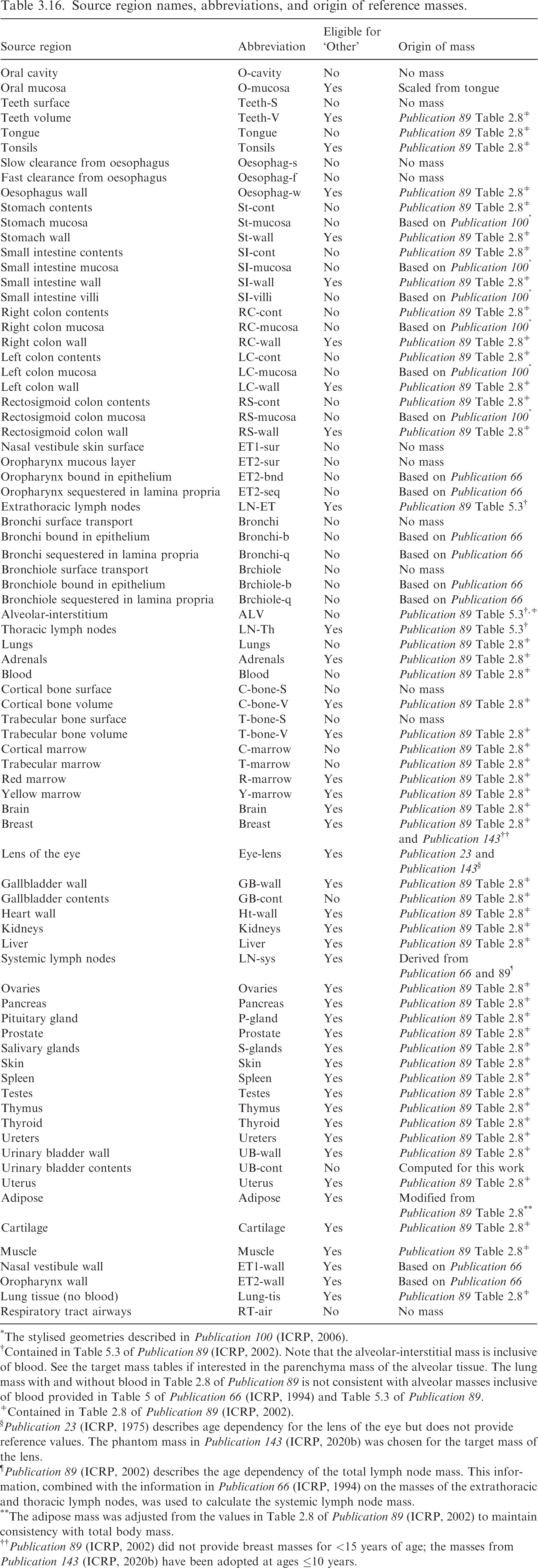
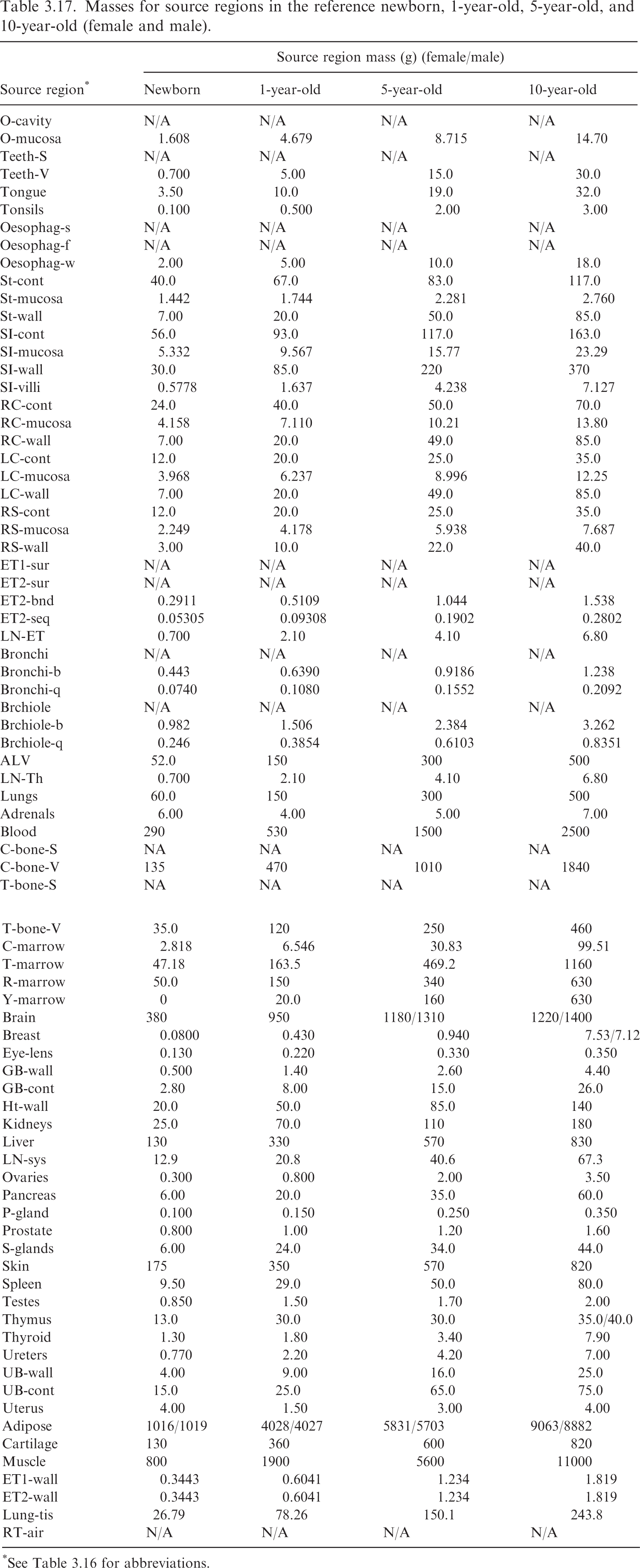
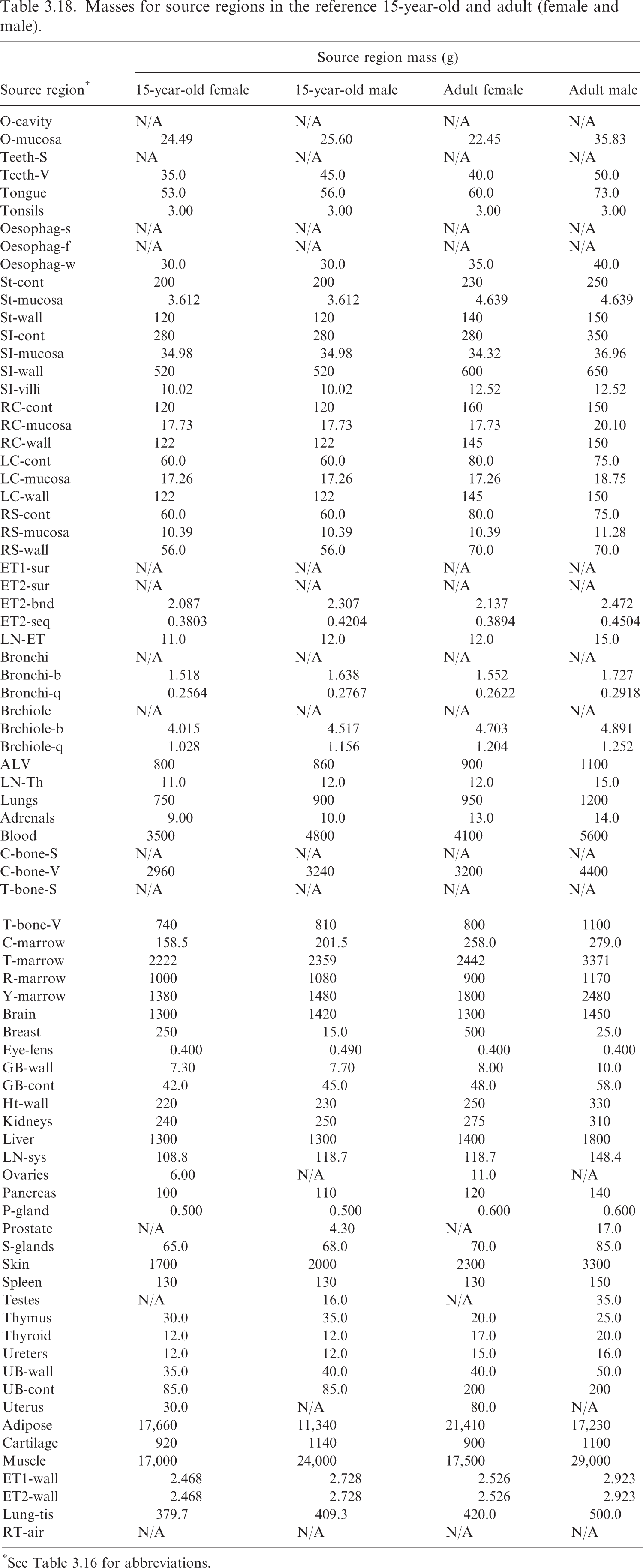
(63) Table 3.16 lists the source regions, their abbreviations, and the basis for the values of their mass. It also provides information as to whether the source region is eligible to be part of ‘Other’ systemic tissue in a biokinetic model. Such tissues are assigned ‘Other’ compartment activity by mass fraction if they are not explicitly invoked elsewhere in the systemic biokinetic model. Note that although ET and TH lymph node regions are typically invoked in the HRTM, they will still be considered part of ‘Other’ if they do not appear in the systemic biokinetic model. Tables 3.17 and 3.18 provide the source region masses for the age-dependent reference individuals.

Table 3.16.

Source region names, abbreviations, and origin of reference masses.

Source region	Abbreviation	Eligible for ‘Other’	Origin of mass
Oral cavity	O-cavity	No	No mass
Oral mucosa	O-mucosa	Yes	Scaled from tongue
Teeth surface	Teeth-S	No	No mass
Teeth volume	Teeth-V	Yes	Publication 89 Table 2.8ǂ
Tongue	Tongue	No	Publication 89 Table 2.8ǂ
Tonsils	Tonsils	Yes	Publication 89 Table 2.8ǂ
Slow clearance from oesophagus	Oesophag-s	No	No mass
Fast clearance from oesophagus	Oesophag-f	No	No mass
Oesophagus wall	Oesophag-w	Yes	Publication 89 Table 2.8ǂ
Stomach contents	St-cont	No	Publication 89 Table 2.8ǂ
Stomach mucosa	St-mucosa	No	Based on Publication 100*
Stomach wall	St-wall	Yes	Publication 89 Table 2.8ǂ
Small intestine contents	SI-cont	No	Publication 89 Table 2.8ǂ
Small intestine mucosa	SI-mucosa	No	Based on Publication 100*
Small intestine wall	SI-wall	Yes	Publication 89 Table 2.8ǂ
Small intestine villi	SI-villi	No	Based on Publication 100*
Right colon contents	RC-cont	No	Publication 89 Table 2.8ǂ
Right colon mucosa	RC-mucosa	No	Based on Publication 100*
Right colon wall	RC-wall	Yes	Publication 89 Table 2.8ǂ
Left colon contents	LC-cont	No	Publication 89 Table 2.8ǂ
Left colon mucosa	LC-mucosa	No	Based on Publication 100*
Left colon wall	LC-wall	Yes	Publication 89 Table 2.8ǂ
Rectosigmoid colon contents	RS-cont	No	Publication 89 Table 2.8ǂ
Rectosigmoid colon mucosa	RS-mucosa	No	Based on Publication 100*
Rectosigmoid colon wall	RS-wall	Yes	Publication 89 Table 2.8ǂ
Nasal vestibule skin surface	ET1-sur	No	No mass
Oropharynx mucous layer	ET2-sur	No	No mass
Oropharynx bound in epithelium	ET2-bnd	No	Based on Publication 66
Oropharynx sequestered in lamina propria	ET2-seq	No	Based on Publication 66
Extrathoracic lymph nodes	LN-ET	Yes	Publication 89 Table 5.3†
Bronchi surface transport	Bronchi	No	No mass
Bronchi bound in epithelium	Bronchi-b	No	Based on Publication 66
Bronchi sequestered in lamina propria	Bronchi-q	No	Based on Publication 66
Bronchiole surface transport	Brchiole	No	No mass
Bronchiole bound in epithelium	Brchiole-b	No	Based on Publication 66
Bronchiole sequestered in lamina propria	Brchiole-q	No	Based on Publication 66
Alveolar-interstitium	ALV	No	Publication 89 Table 5.3†,ǂ
Thoracic lymph nodes	LN-Th	Yes	Publication 89 Table 5.3†
Lungs	Lungs	No	Publication 89 Table 2.8ǂ
Adrenals	Adrenals	Yes	Publication 89 Table 2.8ǂ
Blood	Blood	No	Publication 89 Table 2.8ǂ
Cortical bone surface	C-bone-S	No	No mass
Cortical bone volume	C-bone-V	Yes	Publication 89 Table 2.8ǂ
Trabecular bone surface	T-bone-S	No	No mass
Trabecular bone volume	T-bone-V	Yes	Publication 89 Table 2.8ǂ
Cortical marrow	C-marrow	No	Publication 89 Table 2.8ǂ
Trabecular marrow	T-marrow	No	Publication 89 Table 2.8ǂ
Red marrow	R-marrow	Yes	Publication 89 Table 2.8ǂ
Yellow marrow	Y-marrow	Yes	Publication 89 Table 2.8ǂ
Brain	Brain	Yes	Publication 89 Table 2.8ǂ
Breast	Breast	Yes	Publication 89 Table 2.8ǂ and Publication 143 ††
Lens of the eye	Eye-lens	Yes	Publication 23 and Publication 143§
Gallbladder wall	GB-wall	Yes	Publication 89 Table 2.8ǂ
Gallbladder contents	GB-cont	No	Publication 89 Table 2.8ǂ
Heart wall	Ht-wall	Yes	Publication 89 Table 2.8ǂ
Kidneys	Kidneys	Yes	Publication 89 Table 2.8ǂ
Liver	Liver	Yes	Publication 89 Table 2.8ǂ
Systemic lymph nodes	LN-sys	Yes	Derived from Publication 66 and 89¶
Ovaries	Ovaries	Yes	Publication 89 Table 2.8ǂ
Pancreas	Pancreas	Yes	Publication 89 Table 2.8ǂ
Pituitary gland	P-gland	Yes	Publication 89 Table 2.8ǂ
Prostate	Prostate	Yes	Publication 89 Table 2.8ǂ
Salivary glands	S-glands	Yes	Publication 89 Table 2.8ǂ
Skin	Skin	Yes	Publication 89 Table 2.8ǂ
Spleen	Spleen	Yes	Publication 89 Table 2.8ǂ
Testes	Testes	Yes	Publication 89 Table 2.8ǂ
Thymus	Thymus	Yes	Publication 89 Table 2.8ǂ
Thyroid	Thyroid	Yes	Publication 89 Table 2.8ǂ
Ureters	Ureters	Yes	Publication 89 Table 2.8ǂ
Urinary bladder wall	UB-wall	Yes	Publication 89 Table 2.8ǂ
Urinary bladder contents	UB-cont	No	Computed for this work
Uterus	Uterus	Yes	Publication 89 Table 2.8ǂ
Adipose	Adipose	Yes	Modified from Publication 89 Table 2.8**
Cartilage	Cartilage	Yes	Publication 89 Table 2.8ǂ
Muscle	Muscle	Yes	Publication 89 Table 2.8ǂ
Nasal vestibule wall	ET1-wall	Yes	Based on Publication 66
Oropharynx wall	ET2-wall	Yes	Based on Publication 66
Lung tissue (no blood)	Lung-tis	Yes	Publication 89 Table 2.8ǂ
Respiratory tract airways	RT-air	No	No mass

^*The stylised geometries described in Publication 100 (ICRP, 2006).

^†Contained in Table 5.3 of Publication 89 (ICRP, 2002). Note that the alveolar-interstitial mass is inclusive of blood. See the target mass tables if interested in the parenchyma mass of the alveolar tissue. The lung mass with and without blood in Table 2.8 of Publication 89 is not consistent with alveolar masses inclusive of blood provided in Table 5 of Publication 66 (ICRP, 1994) and Table 5.3 of Publication 89.

^ǂContained in Table 2.8 of Publication 89 (ICRP, 2002).

^§Publication 23 (ICRP, 1975) describes age dependency for the lens of the eye but does not provide reference values. The phantom mass in Publication 143 (ICRP, 2020b) was chosen for the target mass of the lens.

^¶Publication 89 (ICRP, 2002) describes the age dependency of the total lymph node mass. This information, combined with the information in Publication 66 (ICRP, 1994) on the masses of the extrathoracic and thoracic lymph nodes, was used to calculate the systemic lymph node mass.

^**The adipose mass was adjusted from the values in Table 2.8 of Publication 89 (ICRP, 2002) to maintain consistency with total body mass.

^††Publication 89 (ICRP, 2002) did not provide breast masses for <15 years of age; the masses from Publication 143 (ICRP, 2020b) have been adopted at ages ≤10 years.

Table 3.17.

Masses for source regions in the reference newborn, 1-year-old, 5-year-old, and 10-year-old (female and male).

Source region*	Source region mass (g) (female/male)
	Newborn	1-year-old	5-year-old	10-year-old
O-cavity	N/A	N/A	N/A	N/A
O-mucosa	1.608	4.679	8.715	14.70
Teeth-S	N/A	N/A	N/A	N/A
Teeth-V	0.700	5.00	15.0	30.0
Tongue	3.50	10.0	19.0	32.0
Tonsils	0.100	0.500	2.00	3.00
Oesophag-s	N/A	N/A	N/A	N/A
Oesophag-f	N/A	N/A	N/A	N/A
Oesophag-w	2.00	5.00	10.0	18.0
St-cont	40.0	67.0	83.0	117.0
St-mucosa	1.442	1.744	2.281	2.760
St-wall	7.00	20.0	50.0	85.0
SI-cont	56.0	93.0	117.0	163.0
SI-mucosa	5.332	9.567	15.77	23.29
SI-wall	30.0	85.0	220	370
SI-villi	0.5778	1.637	4.238	7.127
RC-cont	24.0	40.0	50.0	70.0
RC-mucosa	4.158	7.110	10.21	13.80
RC-wall	7.00	20.0	49.0	85.0
LC-cont	12.0	20.0	25.0	35.0
LC-mucosa	3.968	6.237	8.996	12.25
LC-wall	7.00	20.0	49.0	85.0
RS-cont	12.0	20.0	25.0	35.0
RS-mucosa	2.249	4.178	5.938	7.687
RS-wall	3.00	10.0	22.0	40.0
ET1-sur	N/A	N/A	N/A	N/A
ET2-sur	N/A	N/A	N/A	N/A
ET2-bnd	0.2911	0.5109	1.044	1.538
ET2-seq	0.05305	0.09308	0.1902	0.2802
LN-ET	0.700	2.10	4.10	6.80
Bronchi	N/A	N/A	N/A	N/A
Bronchi-b	0.443	0.6390	0.9186	1.238
Bronchi-q	0.0740	0.1080	0.1552	0.2092
Brchiole	N/A	N/A	N/A	N/A
Brchiole-b	0.982	1.506	2.384	3.262
Brchiole-q	0.246	0.3854	0.6103	0.8351
ALV	52.0	150	300	500
LN-Th	0.700	2.10	4.10	6.80
Lungs	60.0	150	300	500
Adrenals	6.00	4.00	5.00	7.00
Blood	290	530	1500	2500
C-bone-S	NA	NA	NA	NA
C-bone-V	135	470	1010	1840
T-bone-S	NA	NA	NA	NA
T-bone-V	35.0	120	250	460
C-marrow	2.818	6.546	30.83	99.51
T-marrow	47.18	163.5	469.2	1160
R-marrow	50.0	150	340	630
Y-marrow	0	20.0	160	630
Brain	380	950	1180/1310	1220/1400
Breast	0.0800	0.430	0.940	7.53/7.12
Eye-lens	0.130	0.220	0.330	0.350
GB-wall	0.500	1.40	2.60	4.40
GB-cont	2.80	8.00	15.0	26.0
Ht-wall	20.0	50.0	85.0	140
Kidneys	25.0	70.0	110	180
Liver	130	330	570	830
LN-sys	12.9	20.8	40.6	67.3
Ovaries	0.300	0.800	2.00	3.50
Pancreas	6.00	20.0	35.0	60.0
P-gland	0.100	0.150	0.250	0.350
Prostate	0.800	1.00	1.20	1.60
S-glands	6.00	24.0	34.0	44.0
Skin	175	350	570	820
Spleen	9.50	29.0	50.0	80.0
Testes	0.850	1.50	1.70	2.00
Thymus	13.0	30.0	30.0	35.0/40.0
Thyroid	1.30	1.80	3.40	7.90
Ureters	0.770	2.20	4.20	7.00
UB-wall	4.00	9.00	16.0	25.0
UB-cont	15.0	25.0	65.0	75.0
Uterus	4.00	1.50	3.00	4.00
Adipose	1016/1019	4028/4027	5831/5703	9063/8882
Cartilage	130	360	600	820
Muscle	800	1900	5600	11000
ET1-wall	0.3443	0.6041	1.234	1.819
ET2-wall	0.3443	0.6041	1.234	1.819
Lung-tis	26.79	78.26	150.1	243.8
RT-air	N/A	N/A	N/A	N/A

^*See Table 3.16 for abbreviations.

Table 3.18.

Masses for source regions in the reference 15-year-old and adult (female and male).

Source region*	Source region mass (g)
	15-year-old female	15-year-old male	Adult female	Adult male
O-cavity	N/A	N/A	N/A	N/A
O-mucosa	24.49	25.60	22.45	35.83
Teeth-S	NA	N/A	N/A	N/A
Teeth-V	35.0	45.0	40.0	50.0
Tongue	53.0	56.0	60.0	73.0
Tonsils	3.00	3.00	3.00	3.00
Oesophag-s	N/A	N/A	N/A	N/A
Oesophag-f	N/A	N/A	N/A	N/A
Oesophag-w	30.0	30.0	35.0	40.0
St-cont	200	200	230	250
St-mucosa	3.612	3.612	4.639	4.639
St-wall	120	120	140	150
SI-cont	280	280	280	350
SI-mucosa	34.98	34.98	34.32	36.96
SI-wall	520	520	600	650
SI-villi	10.02	10.02	12.52	12.52
RC-cont	120	120	160	150
RC-mucosa	17.73	17.73	17.73	20.10
RC-wall	122	122	145	150
LC-cont	60.0	60.0	80.0	75.0
LC-mucosa	17.26	17.26	17.26	18.75
LC-wall	122	122	145	150
RS-cont	60.0	60.0	80.0	75.0
RS-mucosa	10.39	10.39	10.39	11.28
RS-wall	56.0	56.0	70.0	70.0
ET1-sur	N/A	N/A	N/A	N/A
ET2-sur	N/A	N/A	N/A	N/A
ET2-bnd	2.087	2.307	2.137	2.472
ET2-seq	0.3803	0.4204	0.3894	0.4504
LN-ET	11.0	12.0	12.0	15.0
Bronchi	N/A	N/A	N/A	N/A
Bronchi-b	1.518	1.638	1.552	1.727
Bronchi-q	0.2564	0.2767	0.2622	0.2918
Brchiole	N/A	N/A	N/A	N/A
Brchiole-b	4.015	4.517	4.703	4.891
Brchiole-q	1.028	1.156	1.204	1.252
ALV	800	860	900	1100
LN-Th	11.0	12.0	12.0	15.0
Lungs	750	900	950	1200
Adrenals	9.00	10.0	13.0	14.0
Blood	3500	4800	4100	5600
C-bone-S	N/A	N/A	N/A	N/A
C-bone-V	2960	3240	3200	4400
T-bone-S	N/A	N/A	N/A	N/A
T-bone-V	740	810	800	1100
C-marrow	158.5	201.5	258.0	279.0
T-marrow	2222	2359	2442	3371
R-marrow	1000	1080	900	1170
Y-marrow	1380	1480	1800	2480
Brain	1300	1420	1300	1450
Breast	250	15.0	500	25.0
Eye-lens	0.400	0.490	0.400	0.400
GB-wall	7.30	7.70	8.00	10.0
GB-cont	42.0	45.0	48.0	58.0
Ht-wall	220	230	250	330
Kidneys	240	250	275	310
Liver	1300	1300	1400	1800
LN-sys	108.8	118.7	118.7	148.4
Ovaries	6.00	N/A	11.0	N/A
Pancreas	100	110	120	140
P-gland	0.500	0.500	0.600	0.600
Prostate	N/A	4.30	N/A	17.0
S-glands	65.0	68.0	70.0	85.0
Skin	1700	2000	2300	3300
Spleen	130	130	130	150
Testes	N/A	16.0	N/A	35.0
Thymus	30.0	35.0	20.0	25.0
Thyroid	12.0	12.0	17.0	20.0
Ureters	12.0	12.0	15.0	16.0
UB-wall	35.0	40.0	40.0	50.0
UB-cont	85.0	85.0	200	200
Uterus	30.0	N/A	80.0	N/A
Adipose	17,660	11,340	21,410	17,230
Cartilage	920	1140	900	1100
Muscle	17,000	24,000	17,500	29,000
ET1-wall	2.468	2.728	2.526	2.923
ET2-wall	2.468	2.728	2.526	2.923
Lung-tis	379.7	409.3	420.0	500.0
RT-air	N/A	N/A	N/A	N/A

^*See Table 3.16 for abbreviations.

4. Models and Methods for Energy Absorption Computation

(64) To compute SAFs, the absorbed fraction requires the computation of the energy absorption in each target per energy emitted from each source region. This computation is performed in a computational model.

(65) For a large number of source-target geometries, the computational models are the reference voxel phantoms provided in Publications 110 and 143 (ICRP, 2009, 2020b). However, there are many smaller regions where a finer, detailed model is required. These include the alimentary tract, the respiratory tract, and the skeleton. The following sections describe the models and the methods used to compute SAFs in those models.

4.1. Reference voxel phantoms

4.1.1. Summary and definition

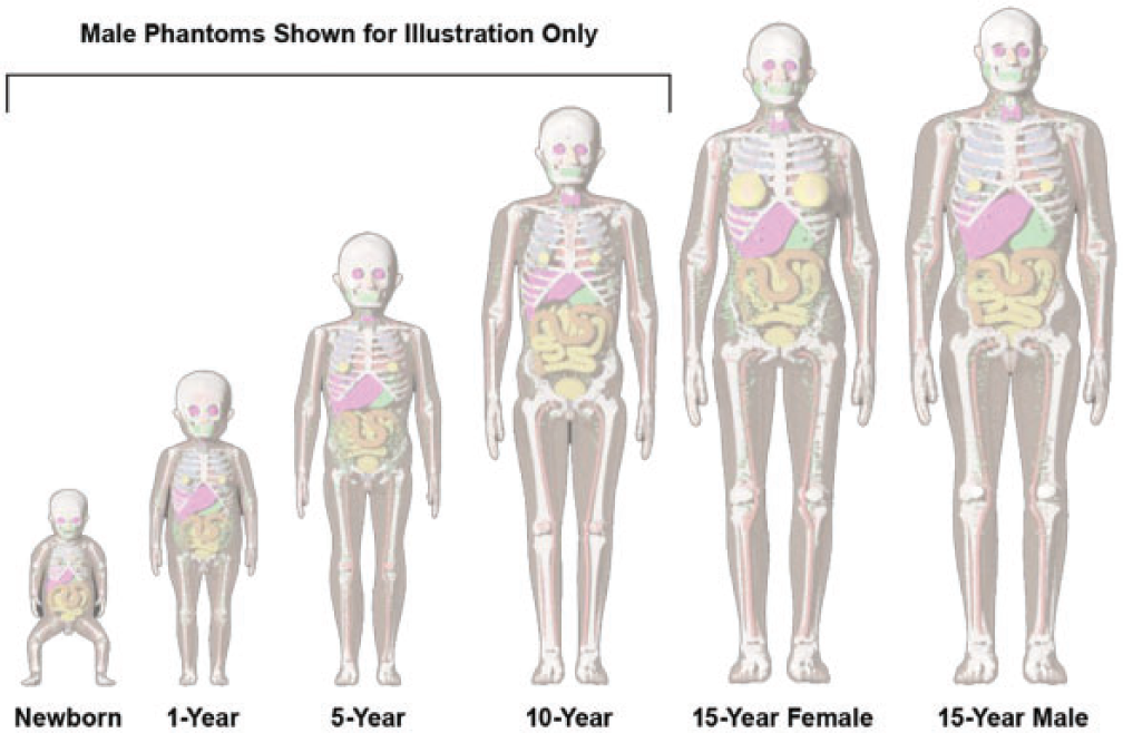
(66) The reference voxel phantoms for the adult are found in Publication 110 (ICRP, 2009), and were adjusted to conform with reference parameters from individuals of similar size (Zankl and Wittmann, 2001; Zankl, 2005). The development of the phantoms is detailed in Publication 110, and the use of the phantom to compute SAFs is described in detail in Publication 133 (ICRP, 2016a). As the SAFs in Publication 133 are adopted as published for this work, the focus in this section will be on the use of the Publication 143 (ICRP, 2020b) phantoms to compute SAFs for the paediatric reference individuals.

(67) The paediatric reference computational phantoms were based on a series of phantoms developed at the University of Florida (UF) and the US National Cancer Institute (Lee et al., 2010). The details of the adjustments made to the phantoms are described in Publication 143 (ICRP, 2020b). The voxelised phantoms are depicted in Fig. 4.1.

(68) While the masses and sizes of the Publication 143 (ICRP, 2020b) phantoms are unique, they were developed to have consistent descriptors as those in Publication 110 (ICRP, 2009; e.g. organs, organ ID numbers, blood contribution to elemental compositions). Body morphometry of the Publication 143 phantoms was based on values provided in Publication 89 (ICRP, 2002). The phantoms are based on medical image data of real individuals, consistent with the reference anatomical information in Publication 89.

Fig. 4.1.

International Commission on Radiological Protection series of reference paediatric voxel computational phantoms from Publication 143 (ICRP, 2020b).

4.1.2. Photons

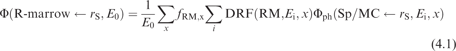
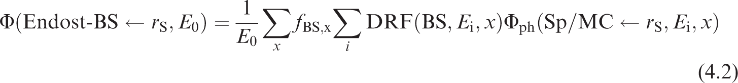
(69) Schwarz et al. (2021b) reported the details for the computation of photon SAFs in the reference paediatric phantoms of Publication 143 (ICRP, 2020b). Monte Carlo photon radiation transport simulations were performed using MCNPX v2.7 (Pelowitz, 2011) in each paediatric reference phantom. In each phantom, 60 tissues served as source and/or target regions. When a desired tissue region did not exist in the reference voxel phantom, surrogate tissues were used to represent the desired tissue. For example, the reference phantoms do not model the thin stem cell target regions in the alimentary tract. The entire stomach wall is thus treated as a surrogate for the stomach stem target.

(70) Monoenergetic photon emissions were simulated from source regions across a logarithmic energy grid from 10 keV to 10 MeV. For non-skeletal source regions, all voxels comprising a source region were sampled uniformly. For skeletal source regions, non-uniform spatial sampling was applied within the various tissues of the paediatric skeleton. As with the Publication 110 (ICRP, 2009) adult phantoms, the skeletal sites of each of the Publication 143 (ICRP, 2020b) phantoms may be composed of both spongiosa (representing a mixture of marrow cavities and bone trabeculae) and cortical bone (the bone cortex). The spongiosa represents four source regions: active marrow (red marrow), inactive marrow (yellow marrow), trabecular bone surface, and trabecular bone volume. Spongiosa regions exist in bones of both the axial and appendicular skeleton. The cortical bone surface and cortical bone volume source regions are simulated as emissions from cortical bone voxels. A table in Schwarz et al. (2021b) contains the fractional distribution of the skeletal tissue regions based on previously published skeletal tissue models (Pafundi et al., 2010; Wayson, 2012).

(71) Energy absorption in red marrow and the bone endosteum were computed for photons by coupling energy-dependent fluence-to-absorbed dose–response functions (Wayson, 2012) to energy-dependent photon fluences scored in the spongiosa (Sp) and medullary cavities (MC) of the long bones. The response functions were derived as described in Johnson et al. (2011). The calculation of SAF, $\text{Φ}$ , to red marrow (RM) and the bone endosteum target (BS, short for bone surface) from photon emission in a source region, $r_{\mathrm{S}}$ , is given in Eqs (4.1) and (4.2):

$$\Phi \left(\text{R-marrow}\leftarrow r_{\text{S}},E_0\right)=\frac{1}{E_0}{\displaystyle \sum _x{f}_{\text{RM,x}}}{\displaystyle \sum _i\text{DRF}\left(\text{RM,}{E}_{\text{i}},x\right){\Phi }_{\text{ph}}\left(\text{Sp/MC}\leftarrow r_{\text{S}},E_{\text{i}},x\right)}$$

(4.1)

$$\Phi \left(\text{Endost-BS}\leftarrow r_{\text{S}},E_0\right)=\frac{1}{E_0}{\displaystyle \sum _x{f}_{\text{BS,x}}}{\displaystyle \sum _i\text{DRF}\left(\text{BS},E_{\text{i}},x\right){\Phi }_{\text{ph}}\left(\text{Sp}/\text{MC}\leftarrow r_{\text{S}},E_{\text{i}},x\right)}$$

(4.2)

(72) The emitted photon energy is $E_0$ , and ${\Phi }_{\text{ph}}\left(\text{Sp}/\text{MC}\leftarrow r_{\text{S}},E_{\text{i}},x\right)$ is the scored photon fluence within the spongiosa or medullary cavity region of bone site x at photon energy $E_{\text{i}}$ . The skeletal dose–response functions, $\text{DRF}\left(\text{RM,}{E}_{\text{i}},x\right)$ and DRF (BS, E_i, x), provide the absorbed dose per unit photon fluence for red marrow and bone endosteum targets, respectively, at each photon energy and within each bone site. The fractional masses of red marrow and bone endosteum within each bone site are provided by $f.$ Tabulated values for the dose–response functions and the fractional masses are provided in the electronic download which accompanies this publication and are described in Annex A.

(73) The inclusion of a blood source region in the latest ICRP biokinetic models necessitates computation of SAFs for emissions from a blood source distributed appropriately across the reference voxel phantoms. Source regions for a blood source should include blood in large vessels, heart contents, and blood perfusing tissue. For the latter region, weighting of all blood-containing tissue source region SAFs can be used to compute a blood SAF as detailed in Eq. (4.3):

$$\Phi \left(r_{\text{T}}\leftarrow \text{Blood},E_0\right)={\displaystyle \sum _S{f}_{\text{Blood,S}}\Phi \left(r_{\text{T}}\leftarrow r_{\text{S}},E_0\right)}$$

(4.3)

where f_Blood,S is the fraction of the body’s blood assigned in a source region, and Φ is the photon SAF for a given source/target combination. The fractional blood distribution is published in Wayson et al. (2018). Further details on the application of this blood distribution to the phantoms are described in Schwarz et al. (2021b).

• (74) Data smoothing was performed for those crossfire geometries at lower energies when relative error in energy deposition tallies exceeds 5% (photons of energies at or below 30 keV). At the lowest energies, log–log extrapolation to theoretical zero energy limiting values (see Section 5.2) was performed. Details of the smoothing methods and when they were applied in each phantom are found in Schwarz et al. (2021b).

4.1.3. Electrons

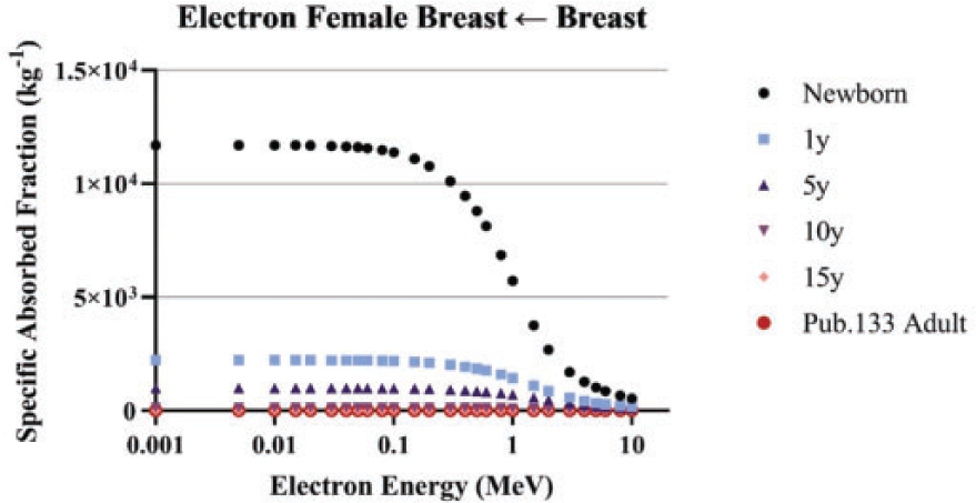
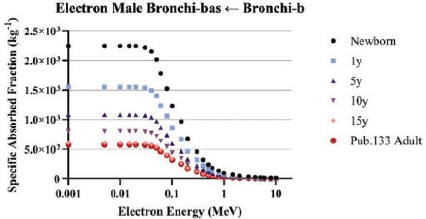
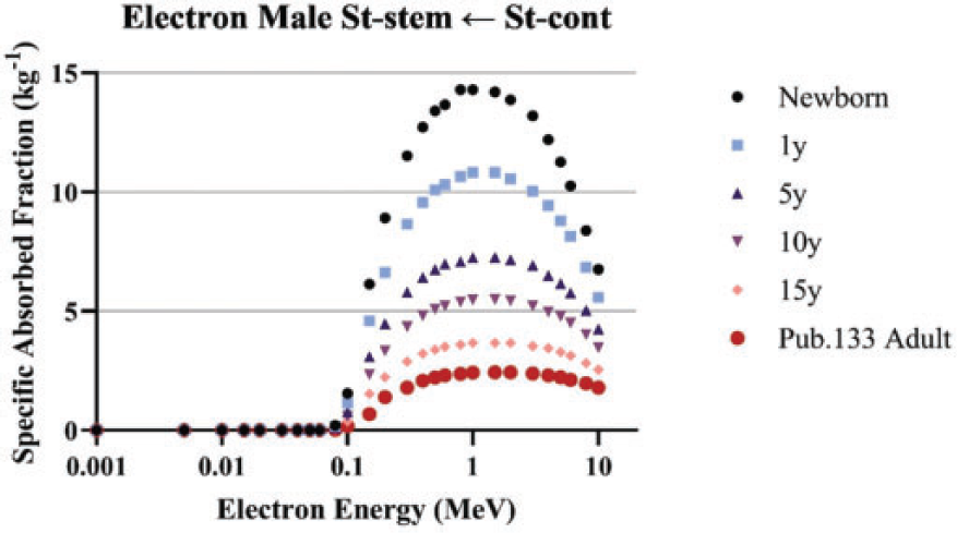
(75) Schwarz et al. (2021a) reported the details for the computation of electron SAFs in the reference paediatric phantoms. Until Publication 133 (ICRP, 2016a) for the adult and this publication for paediatric individuals, electron absorbed fractions were generally treated as either unity for self-irradiation geometries or zero for crossfire geometries. In Publication 133 and in this work, Monte Carlo transport of electrons in the reference phantoms allows for non-unity, non-zero absorbed fractions which vary with electron energy. Emitted electron energy is allowed to escape the source region either in the form of electron kinetic energy or via bremsstrahlung x rays resulting from electron radiative energy losses.

(76) The same logarithmic energy grid used for photons is used for electron SAFs. Collisional and radiative components of the electron SAFs are computed independently with the radiative contribution utilising previously computed photon SAFs (Wayson et al., 2012; Schwarz et al., 2021a). Monte Carlo simulations of the electron transport in the phantoms were performed using MCNPX v2.7 (Pelowitz, 2011). The descriptions of sampling source regions and computing energy absorption in target regions are the same as those described in the previous section for photons.

(77) Schwarz et al. (2021a) computed collisional electron energy absorption during the electron Monte Carlo transport. When a photon associated with bremsstrahlung x-ray production was created, its energy and source region was scored to create an energy distribution in each region. This distribution was subsequently coupled to photon SAFs to compute the SAFs associated with radiative losses. The collisional and radiative SAFs were then summed to arrive at the total electron SAFs presented in this work. The radiative component of the electron SAF was computed as:

$${\Phi }_{\text{R}}\left(r_{\text{T}}\leftarrow r_{\text{S}},E_0\right)=\frac{1}{N_{\text{e}}{E}_0^{\text{e}}}{\displaystyle \sum _i{E}_{\text{i}}^{\text{P}}{\Phi }^{\text{P}}\left(r_{\text{T}}\leftarrow r_{\text{S}},E_{\text{i}}^{\text{P}}\right)}$$

(4.4)

where ${\Phi }^{\text{P}}\left(r_{\text{T}}\leftarrow r_{\text{S}},E_{\text{i}}^{\text{P}}\right)$ is the photon SAF for the source/target pair indexed to the x-ray photon energy $E_{\text{i}}^{\text{P}}$ . The denominator is the product of the number of electrons simulated, $N_{\text{e}}$ , and the emitted electron energy, $E_{\text{0}}^{\text{e}}$ . This approach necessarily presumes that all bremsstrahlung x rays are created interior to the source region, thus neglecting cases where the x ray was generated by an electron which had previously exited the source region boundary. However, in a study by Wayson et al. (2012) using a UF newborn phantom, it was shown that this two-stage approach to computing the electron SAF was statistically comparable with that using full electron transport with explicit bremsstrahlung x-ray production and transport.

• (78) The reference phantoms were not used to derive SAFs for electrons emitted from within skeletal tissues irradiating skeletal targets. The models used for these intraskeletal geometries are described in Section 4.4.2. For electrons emitted from outside the skeleton, the collisional component of the SAF to skeletal targets ${\Phi }_{\text{C}}\left(\text{R-marrow}\leftarrow r_{\text{S}},E_0\right)$ was computed as shown in Eqs (4.5) and (4.6). The fraction of red marrow (or bone endosteum), $f_{\text{RM},\text{x}},$ in each skeletal site, x, is found in Schwarz et al. (2021b). The energy deposited in the spongiosa or medullary cavity region for each skeletal site is $E_{\text{x}}$ .

  $${\Phi }_{\text{C}}\left(\text{R-marrow}\leftarrow r_{\text{S}},E_0\right)=\frac{1}{E_0}{\displaystyle \sum _x{f}_{\text{RM,x}}\left(\frac{E_{\text{x}}}{m_{\text{RM,x}}}\right)}$$

  (4.5)
  $${\Phi }_{\text{C}}\left(\text{Endost-BS}\leftarrow r_{\text{S}},E_0\right)=\frac{1}{E_0}{\displaystyle \sum _x{f}_{\text{BS,x}}\left(\frac{E_{\text{x}}}{m_{\text{BS,x}}}\right)}$$

  (4.6)

• (79) Data smoothing of electron SAFs was found to be unnecessary as the collisional component of the electron SAF had very small statistical errors, and the radiative component utilised photon SAFs which had already been smoothed where necessary. Low energy interpolation to theoretical zero energy SAFs was performed in the same manner (log–log) as described previously for photons.

4.1.4. Neutrons from spontaneous fission

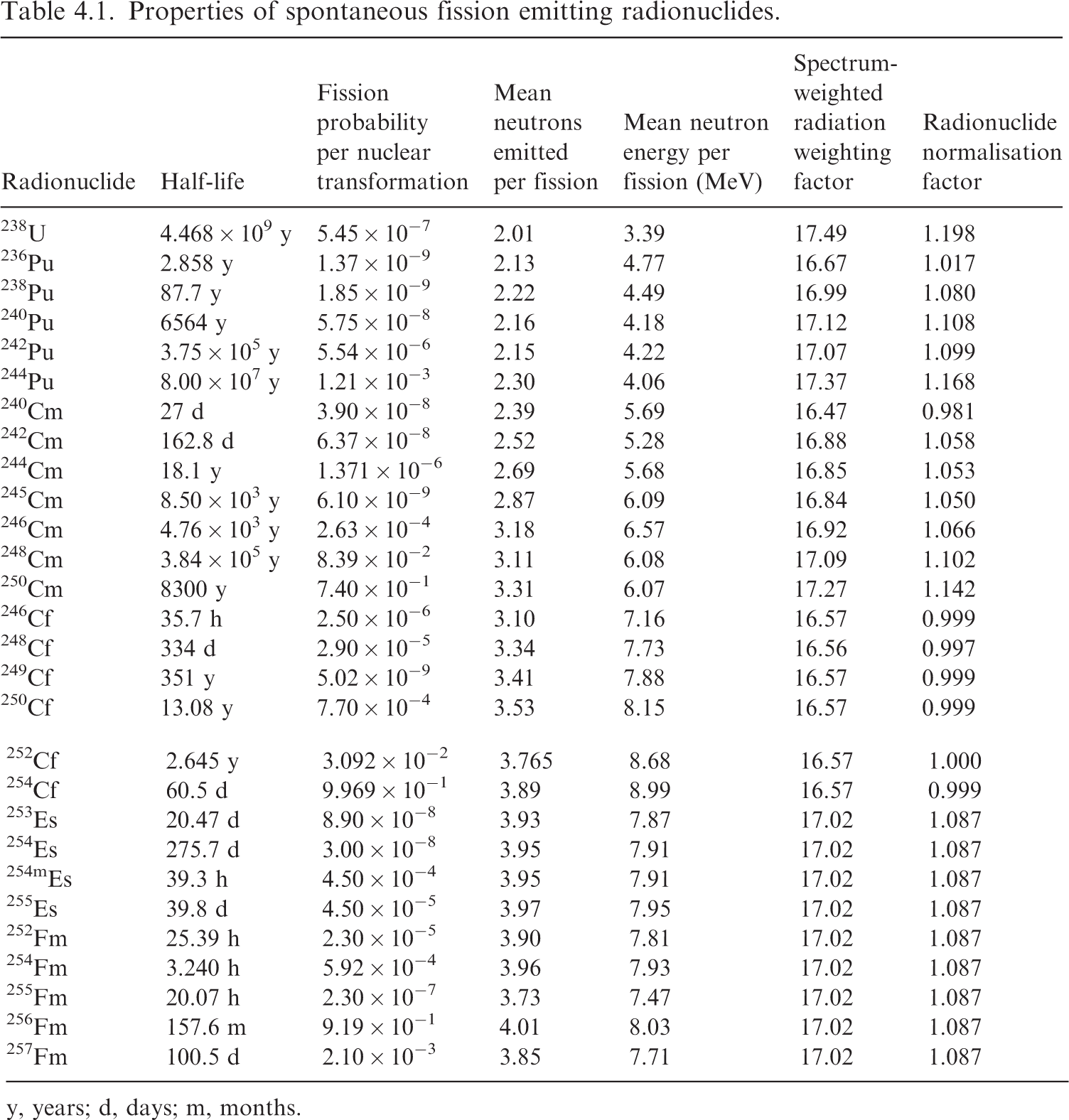
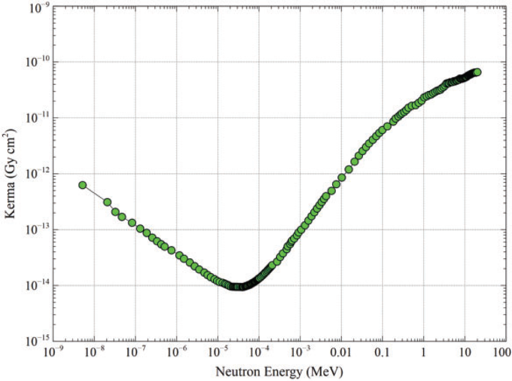
(80) Griffin et al. (2022) reported the details for the computation of SAFs for fission-spectrum neutrons in the reference paediatric phantoms. Neutron SAFs in this publication address 28 radionuclides which undergo spontaneous fission with a branching fraction greater than 1 × 10⁻⁹ per nuclear transformation (ICRP, 2008b). Unlike the other SAFs in this publication, neutron SAFs are computed and tabulated in a manner specific to the radionuclide rather than specific to a grid of monoenergetic emissions. SAFs were calculated for ²⁵²Cf using MCNP6 Version 6.1 (Pelowitz, 2013) in major source regions of the reference voxel phantoms; in other source regions, ²⁵²Cf SAFs were derived using a point-kernel approach. For the remaining 27 radionuclides, the SAFs for ²⁵²Cf were scaled using normalisation factors to account for differences in soft tissue kerma and the average energy of an emitted neutron.

(81) Table 4.1 summarises the decay data information for the selected radionuclides (ICRP, 2008b). The spontaneous fission branching fraction ranges from 1.37 × 10⁻⁹ (²³⁶Pu) to 0.997 (²⁵⁴Cf) per nuclear transformation. The average number of neutrons emitted per fission ranges from 2.01 (²³⁸U) to 4.01 (²⁵⁶Fm). The average emitted neutron energy per fission ranges from 3.39 (²³⁸U) to 8.99 (²⁵⁴Cf) MeV. Note the energy associated with fission fragments greatly exceeds that of the neutrons. For example, the energy of the ²⁵⁶Fm fission fragments is 194.56 MeV. These fragments are assumed to have the same SAF as a 2.0-MeV alpha particle (local absorption).

(82) The neutron SAFs are tabulated by radionuclide and address the energy spectrum of the fission neutrons. As the neutron radiation weighting factors in Publication 103 (ICRP, 2007) are energy-dependent, radiation weighting factors for neutrons from nuclides undergoing spontaneous fission are needed which are nuclide-specific and spectrum-weighted. Nuclide-specific radiation weighting factors were derived assuming the neutron radiation weighting factor expressions in Table 2.3 and the Watt neutron fission spectra defined in Publication 107 (ICRP, 2008b). The resultant spectrum-weighted neutron radiation weighting factors are provided in Table 4.1.

(83) The right-hand column of Table 4.1 lists the nuclide-specific normalisation factors applied to ²⁵²Cf SAF values, which are independent of age. This factor accounts for the difference in soft tissue kerma for the spontaneous fission neutron spectrum of the nuclides relative to that of ²⁵²Cf. Fig. 4.2 shows the dependence of the kerma coefficient as a function of neutron energy. The data of Fig. 4.2 were integrated over the Watt spectra, and the resultant value was normalised to that for ²⁵²Cf. This factor also accounts for the difference in the average energy of an emitted neutron from the nuclide relative to that of ²⁵²Cf. The radionuclide normalisation factor ranges from 0.981 (²⁴⁰Cm) to 1.198 (²³⁸U).

Table 4.1.

Properties of spontaneous fission emitting radionuclides.

Radionuclide	Half-life	Fission probability per nuclear transformation	Mean neutrons emitted per fission	Mean neutron energy per fission (MeV)	Spectrum-weighted radiation weighting factor	Radionuclide normalisation factor
238U	4.468 × 109 y	5.45 × 10−7	2.01	3.39	17.49	1.198
236Pu	2.858 y	1.37 × 10−9	2.13	4.77	16.67	1.017
238Pu	87.7 y	1.85 × 10−9	2.22	4.49	16.99	1.080
240Pu	6564 y	5.75 × 10−8	2.16	4.18	17.12	1.108
242Pu	3.75 × 105 y	5.54 × 10−6	2.15	4.22	17.07	1.099
244Pu	8.00 × 107 y	1.21 × 10−3	2.30	4.06	17.37	1.168
240Cm	27 d	3.90 × 10−8	2.39	5.69	16.47	0.981
242Cm	162.8 d	6.37 × 10−8	2.52	5.28	16.88	1.058
244Cm	18.1 y	1.371 × 10−6	2.69	5.68	16.85	1.053
245Cm	8.50 × 103 y	6.10 × 10−9	2.87	6.09	16.84	1.050
246Cm	4.76 × 103 y	2.63 × 10−4	3.18	6.57	16.92	1.066
248Cm	3.84 × 105 y	8.39 × 10−2	3.11	6.08	17.09	1.102
250Cm	8300 y	7.40 × 10−1	3.31	6.07	17.27	1.142
246Cf	35.7 h	2.50 × 10−6	3.10	7.16	16.57	0.999
248Cf	334 d	2.90 × 10−5	3.34	7.73	16.56	0.997
249Cf	351 y	5.02 × 10−9	3.41	7.88	16.57	0.999
250Cf	13.08 y	7.70 × 10−4	3.53	8.15	16.57	0.999
252Cf	2.645 y	3.092 × 10−2	3.765	8.68	16.57	1.000
254Cf	60.5 d	9.969 × 10−1	3.89	8.99	16.57	0.999
253Es	20.47 d	8.90 × 10−8	3.93	7.87	17.02	1.087
254Es	275.7 d	3.00 × 10−8	3.95	7.91	17.02	1.087
254mEs	39.3 h	4.50 × 10−4	3.95	7.91	17.02	1.087
255Es	39.8 d	4.50 × 10−5	3.97	7.95	17.02	1.087
252Fm	25.39 h	2.30 × 10−5	3.90	7.81	17.02	1.087
254Fm	3.240 h	5.92 × 10−4	3.96	7.93	17.02	1.087
255Fm	20.07 h	2.30 × 10−7	3.73	7.47	17.02	1.087
256Fm	157.6 m	9.19 × 10−1	4.01	8.03	17.02	1.087
257Fm	100.5 d	2.10 × 10−3	3.85	7.71	17.02	1.087

y, years; d, days; m, months.

Fig. 4.2.

Neutron kerma coefficient (Gy cm²) in soft tissue as a function of neutron energy (Howerton, 1986).

4.1.5. Alpha particles

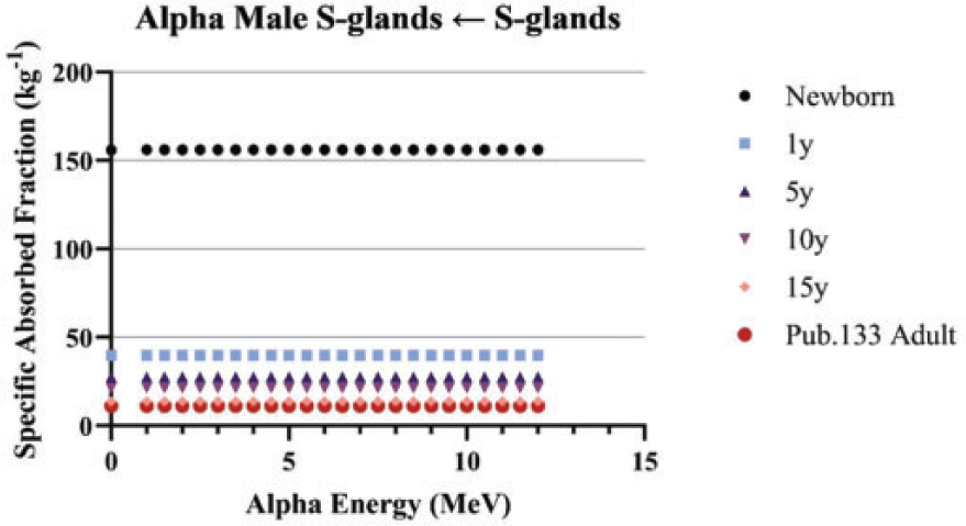
(84) Unlike electron transport simulations in the reference phantoms, alpha particle transport simulations are unnecessary due to the short range of alpha particles compared with the size of the source regions. For such geometries, the alpha absorbed fraction is set to unity for self-irradiation geometries and zero for non-overlapping source-target geometries (crossfire geometries). The resulting alpha SAF for the self-irradiation geometries is simply the inverse of the target region mass. These values are applied at all alpha particle energies (up to 12 MeV). The kinetic energy of the recoiling nucleus, typically approximately 2% of alpha particle energy, is assumed to inherit the SAF of a 2.0-MeV alpha particle (local absorption).

4.2. Alimentary tract

4.2.1. Summary and definition

(85) The computational models used to compute SAFs within the alimentary tract are based on the geometrical definitions provided in Section 7 of Publication 100 (ICRP, 2006). For each region in the alimentary tract, information is provided on the simplified geometrical shape and the sizes of these regions. Tables 3.6 and 3.7 summarise some of this information for the various target regions. Similar information is provided in Publication 100 which defines the location and size of various source regions.

4.2.2. Electrons and alpha particles

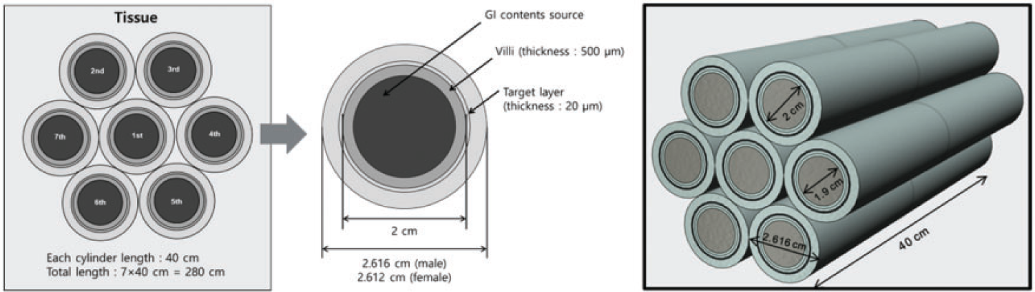
(86) Annex F of Publication 100 (ICRP, 2006) provided electron SAF values based upon Monte Carlo radiation transport simulation in the geometrical models. Similar simulations were not provided for alpha particles. For Publication 133 (ICRP, 2016a), new radiation transport simulations were performed for both electron and alpha particles using the geometries from Publication 100 with one modelling improvement made to the small intestine. Rather than modelling the small intestine as a single cylinder, the cylinders were stacked in a hexagonal array to allow for energy deposition across one segment of the small intestine to another nearby segment. Fig. 4.3 depicts the geometry used for the small intestine.

(87) The same approach used in Publication 133 (ICRP, 2016a) has been extended in this work using the age-specific geometry information provided in Publication 100 (ICRP, 2006) for both electrons (up to 10 MeV) and alpha particles (up to 12 MeV).

Fig. 4.3.

Schematic of the folded small intestine model used to allow for electron crossfire. GI, gastrointestinal.

4.2.3. Photons and neutrons

(88) For photons and neutrons, surrogate tissues in the reference phantom were used to represent the small source and target regions in the alimentary tract. For example, the SAF to desired stem cell targets is considered to be the same as the SAF to the encompassing, corresponding wall region. Similarly, a photon or neutron source emanating from an alimentary mucosal region is treated as originating from the wall in the reference voxel phantom.

4.3. Respiratory tract

4.3.1. Summary and definition

(89) Publication 66 (ICRP, 1994) contains information on the morphometrical model used to define computational models for regions inside the respiratory tract. While the publication contains some information on age and sex dependency, for dosimetric modelling, the cross-sectional dimensions of the airway regions (airway and wall thicknesses) have been treated as independent of age and sex. Thus, the absorbed fractions computed for the adults are applied at all younger ages. The SAF then changes by the mass of the target region which is dependent on age and sex.

4.3.2. Electrons and alpha particles

(90) Section 5 of Publication 133 (ICRP, 2016a) describes the adoption of respiratory tract SAFs previously provided in Publication 66 (ICRP, 1994) in Annex H. In the first part of the OIR series, Publication 130 (ICRP, 2015), revisions were made to the respiratory tract model. The original HRTM included particle-size-dependent slow clearance compartments which were eliminated in the revision. The revised source region is taken to be distributed uniformly throughout both the gel and sol layers of Publication 66. The weights for the relative thickness of the gel and sol are 5/11 and 6/11, respectively, for the bronchial region, and 1/3 and 2/3, respectively, for the bronchiolar region.

(91) Publication 133 (ICRP, 2016a) also describes the addition of new electron SAFs for geometries based on radiation transport in the reference voxel phantoms. This was used for AI and ET lymph node source regions. Alpha SAFs were not updated in this manner, but were instead adopted as they appear in Publication 66 (ICRP, 1994).

4.3.3. Photons and neutrons

(92) For photons and neutrons, surrogate tissues in the reference phantom were used to represent the small source and target regions in the respiratory tract. For example, the SAFs to secretory targets in the bronchi were considered to be the same as the SAFs to the bronchi wall region. Similarly, a photon or neutron source emanating from the AI is treated as coming from the whole lung in the reference voxel phantom.

4.4. Skeleton

4.4.1. Summary and definition

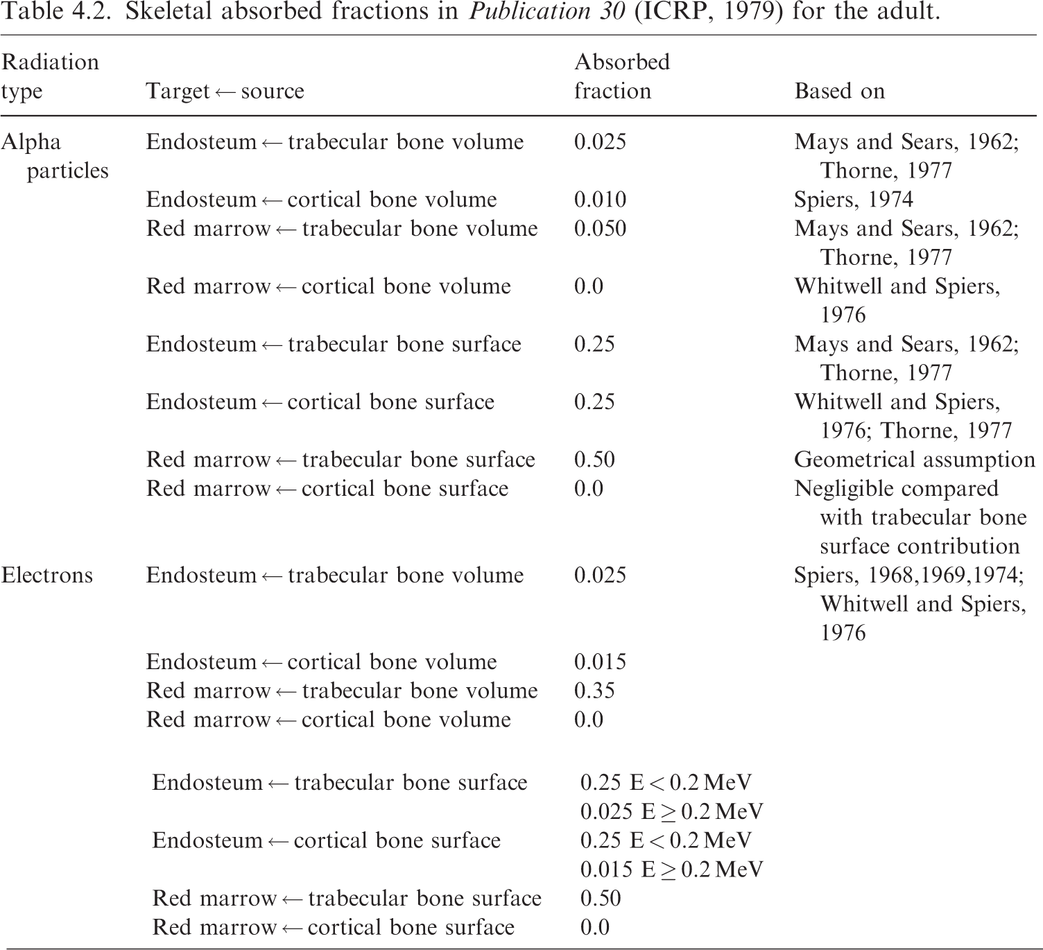
(93) Publication 11 (ICRP, 1968) defined three cellular regions at risk for radiogenic damage within the skeleton: cells among the osteogenic cells on bone surfaces; haematopoietic marrow; and certain epithelial cells close to bone surfaces. The same publication defined the dose to the latter category as averaged over the region ‘… from 5 to 10 µm from the trabecular surface’. Publication 26 (ICRP, 1977) includes a recommendation that the ‘… dose equivalent in bone should apply to the endosteal cells and cells on bone surfaces, and should be calculated as an average over tissue up to a distance of 10 µm from the relevant bone surfaces’. Publication 30 (ICRP, 1979) uses the 10-µm recommendation from Publication 26.

(94) More recently, studies have shown that the cells at risk for bone cancer induction are localised up to 50 µm from trabecular and interior cortical bone surfaces (Gossner et al., 2000; Gossner, 2003; Bolch et al., 2007). In this work and in Publication 133 (ICRP, 2016a), the bone endosteum target is considered to be all marrow tissue within 50 µm of a trabecular surface or interior cortical bone surface along the shafts of the long bones.

(95) Data suggest that haematopoietic stem cells are found preferentially near trabecular bone surfaces (Watchman et al., 2007; Bourke et al., 2009). Nevertheless, in this work, as in Publication 133 (ICRP, 2016a), dosimetric modelling treats the cells as uniformly distributed among the marrow spaces. The models used do explicitly treat red and yellow marrow as separate, interspersed regions within the marrow spaces.

(96) Publication 20 (ICRP, 1973) describes the basis for the definition of skeletal source regions. Rowland (1966) describes rapidly exchangeable calcium of bone as located at bone surfaces alone, which include cortical and trabecular endosteum, periosteum, and the surfaces of Haversian and Volkmann canals. Publication 20 (ICRP, 1973) states ‘The calcium which lies within less than one micron from a bone surface was found to be sufficient to account for the size and location of the observed exchangeable pool’. Publication 20 also describes the splitting of activity in the bone between cortical and trabecular regions of the skeleton as being split by the fraction of cortical/trabecular bone in the whole-body skeleton (80%/20%). This value was later affirmed in Publication 70 (ICRP, 1995a).

(97) For the dosimetry in Publication 30 (ICRP, 1979), as well as the dosimetry here, radionuclides assumed to be on bone surfaces are modelled as uniformly spread in an infinitely thin layer over the relevant surfaces of bone. Importantly, Publication 30 states ‘This assumption will result in an over-estimate of the true committed dose equivalents received by bone surface cells and active bone marrow because it disregards burial of radioactive deposits by the deposition of new bone mineral’.

(98) The absorbed fraction of alpha particle energy emitted from skeletal regions was described in Publication 30 (ICRP, 1979). These values were used in subsequent ICRP dosimetry calculations. Several studies have found energy dependency in intraskeletal absorbed fractions for electrons (Spiers, 1970; Eckerman et al., 1985; Bouchet et al., 1999; Eckerman and Stabin, 2000; Jokisch et al., 2001; Patton et al., 2002; Shah et al., 2005; Kramer et al., 2012; Dant et al., 2013; Gao et al., 2017; Degteva et al., 2021) and alpha particles (Thorne, 1976; Watchman et al., 2005; Hunt et al., 2007; Watchman and Bolch, 2009). Publication 106 (ICRP, 2008a) represented the first departure from the electron absorbed fraction values of Publication 30 and shown in Table 4.2. Publication 106 used values for the adult from Stabin and Siegel (2003), which were based on work by Eckerman and Stabin (2000) and Bouchet et al. (2000), and were described in Stabin et al. (2002). In Publication 30, the reference target masses for the red marrow and bone endosteum were 1.5 and 0.12 kg, respectively.

Table 4.2.

Skeletal absorbed fractions in Publication 30 (ICRP, 1979) for the adult.

Radiation type	Target ← source	Absorbed fraction	Based on
Alpha particles	Endosteum ← trabecular bone volume	0.025	Mays and Sears, 1962; Thorne, 1977
	Endosteum ← cortical bone volume	0.010	Spiers, 1974
	Red marrow ← trabecular bone volume	0.050	Mays and Sears, 1962; Thorne, 1977
	Red marrow ← cortical bone volume	0.0	Whitwell and Spiers, 1976
	Endosteum ← trabecular bone surface	0.25	Mays and Sears, 1962; Thorne, 1977
	Endosteum ← cortical bone surface	0.25	Whitwell and Spiers, 1976; Thorne, 1977
	Red marrow ← trabecular bone surface	0.50	Geometrical assumption
	Red marrow ← cortical bone surface	0.0	Negligible compared with trabecular bone surface contribution
Electrons	Endosteum ← trabecular bone volume	0.025	Spiers, 1968,1969,1974; Whitwell and Spiers, 1976
	Endosteum ← cortical bone volume	0.015
	Red marrow ← trabecular bone volume	0.35
	Red marrow ← cortical bone volume	0.0
	Endosteum ← trabecular bone surface	0.25 E < 0.2 MeV 0.025 E ≥ 0.2 MeV
	Endosteum ← cortical bone surface	0.25 E < 0.2 MeV0.015 E ≥ 0.2 MeV
	Red marrow ← trabecular bone surface	0.50
	Red marrow ← cortical bone surface	0.0

(99) Marrow cellularity is defined as the fraction of bone marrow volume that is haematopoietically active. Cellularity varies by location in the skeleton. Cellularity is also known to vary by age. In this work, reference values for marrow cellularity have been adopted from Table 41 of Publication 70 (ICRP, 1995a). The data are based largely on a review performed by Cristy (1981) of various studies of active marrow distribution. Fig. 4.4 contains a plot of these reference cellularities, and how they vary by skeletal site and age.

Fig. 4.4.

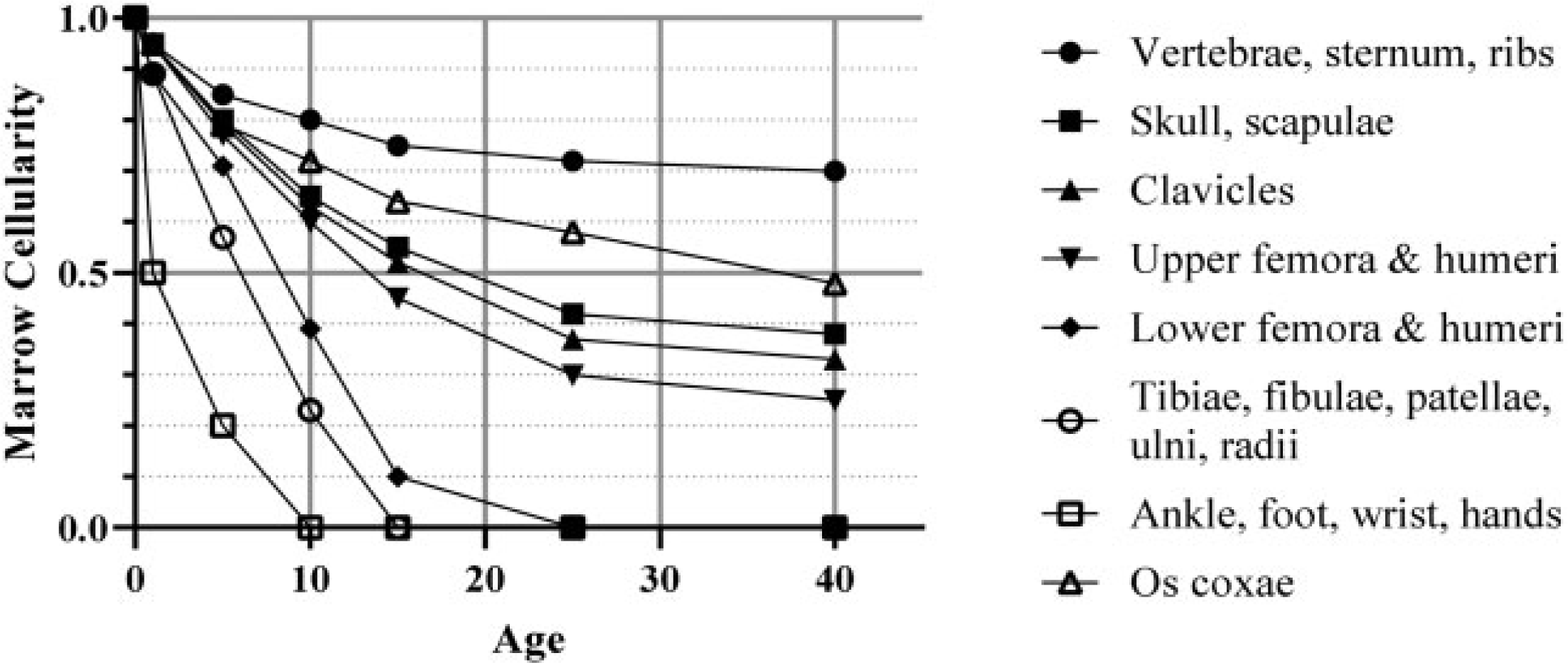
Reference marrow cellularity of Publication 70 (ICRP, 1995a) by skeletal site and age.

4.4.2. Electrons

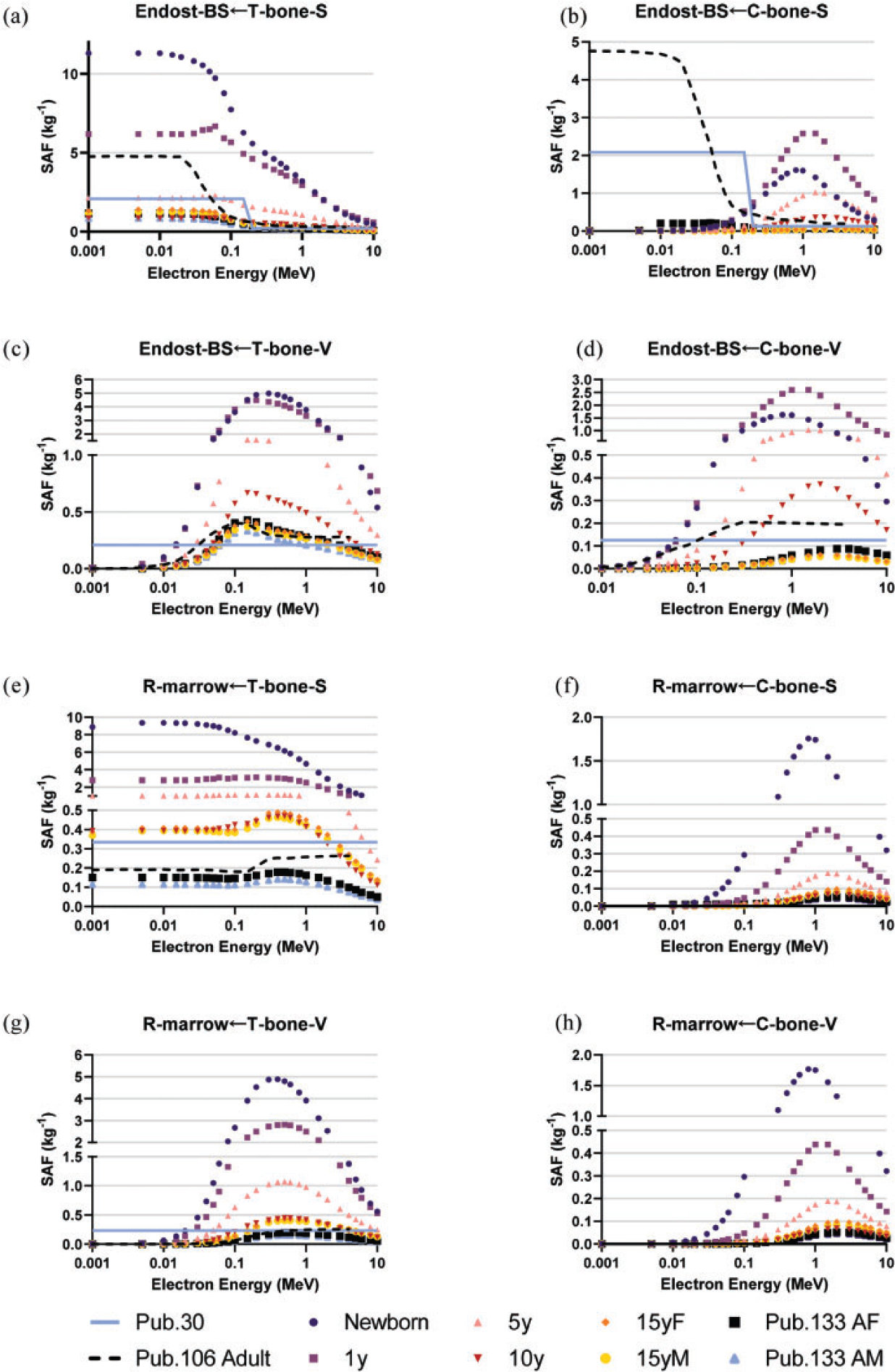
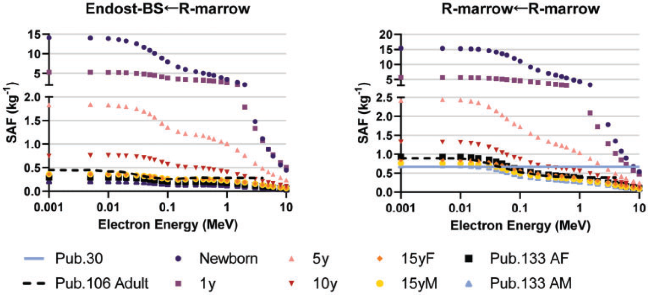
(100) As the microstructure of the skeleton cannot be modelled in the reference voxel phantoms, separate image-based voxel models of human skeletal microstructure have been used to compute absorbed fractions in the adult (Hough et al., 2011; O'Reilly et al., 2016) and paediatric individuals (Pafundi et al., 2010).

(101) Intraskeletal electron SAFs in this work are taken from those developed by Pafundi (2009), and are given as a function of reference age with no differentiation by sex. As described by Pafundi et al. (2009, 2010), electron SAFs were computed following paired-image radiation transport simulation within computed tomography (CT)-based images of whole bone and microCT images of spongiosa cores acquired in five skeletal sites within two female newborns at autopsy. The bone sites were the sternum, occipital bone, ribs, thoracic vertebrae, and lumbar vertebrae. SAF values at bone sites for which a three-dimensional (3D) voxelised model was not available were estimated using weighting schemes originally proposed by Whitwell (1973). For the 15-year model, intraskeletal electron SAFs were based upon paired-image radiation transport simulations within CT and microCT images of some 26 skeletal sites across both the axial and appendicular skeleton of an 18-year-old male cadaver. Methods applied to this model were identical to those described in both Hough et al. (2011) and O’Reilly et al. (2016) for the UF reference adult male and reference adult female, respectively.

(102) As physical samples of trabecular spongiosa were not available to perform 3D electron transport in the skeletons of the 1-year-old, 5-year-old, and 10-year-old reference children, an alternative approach was taken. Macroscale electron transport was first performed within the skeletal sites of the reference phantoms at these three ages to compute sources in the cortical bone, trabecular spongiosa, and medullary cavities of the long bones. Next, microscale electron transport was performed for the 1-year-old and 10-year-old reference children using optical pathlength distributions originally reported by Beddoe et al. (1976) for a 1.7-year-old and 9-year-old child in simulated 3D geometries as described by Watchman et al. (2005). Pathlength distributions within the 5-year model were established as age-interpolated values between the 1.7-year and 9-year datasets.

(103) Fig. 4.5 plots the electron SAFs in this work along with those for the adult from Publications 30, 106, and 133 (ICRP, 1979, 2008a, 2016a). The SAF to the bone surface target is significantly smaller than values used in Publications 30 and 133 due to the previously mentioned change in the target thickness from 10 µm to 50 µm. A significant difference in the definition of the cortical bone source is observed in Fig. 4.5(b). In the present work for electrons, the cortical bone surface was modelled as consisting of Haversian canals within the bone cortex, and the endosteal surface of cortical bone of the long bone shafts. As Haversian canals exist throughout the cortical bone volume, the electron SAFs for cortical bone surfaces are assumed to be identical to those of the cortical bone volume.

(104) The intraskeletal electron SAFs for emissions from the red marrow are shown in Fig. 4.6. The red marrow self-irradiation geometry was treated as independent of energy in Publication 30 (ICRP, 1979). The current models now account for energy-dependent loss to surrounding yellow marrow and bone. The age dependency accounts for the variation in marrow cellularity with age.

Fig. 4.5.

Intraskeletal electron specific absorbed fractions (SAFs) for each reference individual. The plots also show adult SAF values from Publications 30 and 106 (ICRP, 1979, 2008a). Endost-BS, endosteal bone surface; R-marrow, red marrow; T-bone-V, trabecular bone volume; C-bone-V, cortical bone volume; T-bone-S, trabecular bone surface; C-bone-S, cortical bone surface; Pub., Publication; y, years; F, female; M, male; AF, adult female; AM, adult male.

Fig. 4.6.

Intraskeletal electron specific absorbed fractions (SAFs) for each reference individual for emission from the red marrow. Endost-BS, endosteal bone surface; R-marrow, red marrow; Pub., Publication; y, years; F, female; M, male; AF, adult female; AM, adult male.

4.4.3. Alpha particles

(105) Intraskeletal alpha particle SAFs for the adults were computed using both Monte Carlo and range energy type calculations as described in Publication 133 (ICRP, 2016a). Results using similar methods were not available for alpha particles in the paediatric skeleton. One approach for obtaining paediatric SAFs would be to scale the adult SAFs by the target mass. However, the significant changes in the skeletal structures and marrow cellularity with age make this problematic. Instead, an approach was adopted which uses electron SAFs for similarly ranged alpha particles. The method has the benefit of using electron SAF data which account for age-dependent changes in the skeleton. The weakness of the method is that the stopping power is not the same for similarly ranged alpha particles and electrons.

(106) Fig. 4.7 plots the energy of alpha particles and electrons vs their range in red marrow. Each set of data has been fit to obtain empirical power functions relating range and energy for each radiation type. Eqs (4.7) and (4.8) give an empirical range energy equation for each radiation in red marrow, where E is the energy in MeV of the given radiation type and R is the linear range in cm:

$$E_{\text{alpha,RM}}=210R^{0.6678}$$

(4.7)

$$E_{\text{electron,RM}}=1.197R^{0.5757}$$

(4.8)

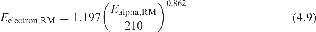
(107) Combining Eqs (4.7) and (4.8) and eliminating the range gives Eq. (4.9), which provides the energy of an electron with equivalent range in red marrow to that of an alpha particle of given energy. Eq. (4.9) is used to obtain electron energies with equivalent ranges to each desired alpha energy on the SAF grid. The SAF is then obtained by interpolating the skeletal electron SAFs:

$$E_{\text{electron,RM}}=1.197{\left(\frac{E_{\text{alpha,RM}}}{210}\right)}^{0.862}$$

(4.9)

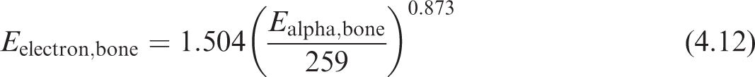
(108) Eq. (4.9) was used to obtain alpha SAFs for emissions from all marrow regions and bone surfaces as the energy absorption is occurring on the soft tissue side of the bone marrow surface plane. An exception was made for the red marrow self-irradiation geometry. For this geometry, adult SAF values were scaled by target mass to the younger ages to preserve consistency of shape of the SAF curve.

(109) Fig. 4.8 shows the ranges of alpha particles and electrons in bone. Eqs (4.10) and (4.11) show empirical relationships between energy and range. Combining these equations and eliminating the range gives Eq. (4.12), which relates the alpha energy to the electron energy which would yield the same range in bone. This equation was used to find interpolated SAFs for emissions from the trabecular bone volume. Note that alpha particles emitted from the cortical bone volume are considered to have absorbed fractions of zero at all alpha energies:

$$E_{\text{alpha,bone}}=259R^{0.6617}$$

(4.10)

$$E_{\text{electron,bone}}=1.504R^{0.5777}$$

(4.11)

$$E_{\text{electron,bone}}=1.504{\left(\frac{E_{\text{alpha,bone}}}{259}\right)}^{0.873}$$

(4.12)

(110) The intraskeletal alpha particle SAFs are shown in Fig. 4.9. As with electrons, significant differences are seen resulting from the change in the modelling definition to a 50-µm endosteum target. For alpha emissions in red marrow, energy loss to surrounding yellow marrow and bone is less significant, but does still show energy dependency. Fig. 4.10 displays values of the SAF for a red marrow source of alpha particles.

Fig. 4.7.

Energy vs range in red marrow for alpha particles and electrons.

Fig. 4.8.

Energy vs range in bone for alpha particles and electrons.

Fig. 4.9.

Intraskeletal alpha particle specific absorbed fractions (SAFs) from bone source regions. Note that y-axis scales are varied to improve visualisation. Endost-BS, endosteal bone surface; R-marrow, red marrow; T-bone-V, trabecular bone volume; C-bone-V, cortical bone volume; T-bone-S, trabecular bone surface; C-bone-S, cortical bone surface; Pub., Publication; y, years; F, female; M, male; AF, adult female; AM, adult male.

Fig. 4.10.

Skeletal specific absorbed fractions (SAFs) for alpha particles emitted from the red (active) marrow. Endost-BS, endosteal bone surface; R-marrow, red marrow; Pub., Publication; y, years; F, female; M, male; AF, adult female; AM, adult male.

4.4.4. Photons and neutrons

(111) SAFs to the skeletal targets for both intraskeletal and extraskeletal photon sources were computed by coupling: (1) Monte-Carlo-derived energy/bone-dependent volumetric photon fluences scored within regions of trabecular spongiosa and long bone medullary marrow cavities; and (2) energy/bone site-dependent fluence-to-dose-response functions for red marrow and endosteum. Adult skeletal dose–response functions (ICRP, 2010, 2016a) were originally computed by Wayson (2012), using the electron SAFs and skeletal tissue masses given in Pafundi (2009) via the methods of Johnson et al. (2011) established for adult photon skeletal dosimetry and used as described here in Eqs (4.1) and (4.2). Age-dependent photon skeletal dose–response functions were used in the computation of photon SAFs.

(112) In Publication 133 (ICRP, 2016a), SAFs to skeletal targets (red marrow and endosteum) for neutrons from spontaneous fission sources were computed by coupling Monte-Carlo-derived neutron fluences to neutron fluence-to-dose-response functions (Bahadori et al., 2011). Similarly, neutron-induced photon fluences, from (n, γ) reactions, were coupled to adult photon fluence-to-dose-response functions (Eckerman et al., 2008; Johnson et al., 2011). For the reference paediatric individuals, the age-dependent photon fluence-to-dose response functions were coupled to the neutron-induced photon fluences from (n, γ) reactions. Fluence-to-dose-response functions for neutron fluences in paediatric individuals were not available, so those derived for the adult male were used instead.

5. Specific Absorbed Fraction Calculation and Tabulation

(113) As described by Eq. (2.14), the SAF is determined by taking the fraction of emitted energy within a source region which is absorbed in a target region and dividing by the mass of the target region. Section 4 described the computational methods and models used to arrive at the absorbed fraction for each source-target combination. Division by the target mass is then performed to provide a SAF. This section describes what adjustments, if any, are made to SAFs computed in models. It also describes methods for quality assurance in this large data set.

5.1. Scaling SAFs to reference mass

(114) While the computational models detailed in Section 4 were designed based on the definitions of the reference individuals of Section 3, the target mass used to compute a SAF in a given model is not always consistent with the reference target mass. In such cases, adjustment of the model-derived SAFs needs to be considered to arrive at the reference SAFs.

(115) The need to consider scaling SAFs from a model or phantom to conform to another individual, whether it be a reference individual, a specific worker, a member of the public, or a medical patient, is not new or unique to this effort. Snyder (1970) wrote about this need in what he described as a ‘preliminary’ discussion which he hoped would spur further study. Snyder proposed a scaling for photon absorbed fractions in self-irradiation geometries which was proportional to the cube root of the mass of the source (and target) region. Snyder found that the proportionality worked well over the region where Compton scattering predominates. Snyder wrote:

Clearly, this rule fails badly for photons of energy below 50 keV, and in these cases the AF [absorbed fraction] is greater than 0.5. Perhaps this reveals at once the limitations of this principle – namely, the organ must be small in relation to the mean free path of the photons that buildup is not an important contribution to the dose or to AF, and thus the principle does not hold for low energies. Clearly, for low photon energies such that the AF is approximately 1, the AF cannot continue to increase with the cube root of the mass as the mass of the organ is increased. Thus, the principle should be applied only for the energy region where Compton scattering predominates and then only when the AF is well below 1, say, ≤0.5. But for many body organs and for a range of photon energies from, say, 0.2 to 2 MeV, the principle seems to hold fairly well.

It should be understood that no claim to a high degree of accuracy is made for these methods; indeed, quite the reverse. It is evident that only a rough approximation to the dose is given.

(116) The Medical Internal Radiation Dose (MIRD) Committee, in MIRD Pamphlet 11 (Snyder et al., 1975), presented the proportionality above in terms of the SAF or absorbed dose as being equivalently proportional to the inverse of the mass to the 2/3 power. Again, the proportionality was qualified as being useful for photons ‘…with energies above 100 keV’:

Since dose from electrons scales with the inverse first power of the mass, if one assumes complete absorption of energy, scaling is no longer simple; the photon dose changes with one power of the mass and the electron dose changes with another. In fact, there seems to be no simple scaling procedure which is approximately correct for all energies of particles and masses of organs.

(117) Adams (1981) described the use of linear mass scaling for photon energies <30 keV, and the inverse 2/3 power scaling for energies >30 keV. Petoussi-Henss et al. (2007) found that photon self-dose SAFs vary with the inverse 2/3 power of mass for energies >100 keV ‘… and for organs that are not extended’. Wayson and Bolch (2018) performed Monte Carlo radiation transport in spheres of varying sizes for photons and electrons. For photon self-dose, they found mass proportionality which varies from the inverse first power (at approximately 10 keV) to the inverse 2/3 power (at 100 keV) and powers less than 2/3 when photon energy exceeds 1 MeV. For electrons, the same study found that the SAF was proportional to the inverse of the mass for all energies up to approximately 1 MeV.

5.1.1. Self-irradiation geometries

(118) Self-irradiation geometries are defined here as any in which the low energy SAF is non-zero. These include source and target region being identical, but also include overlapping source and target regions.

(119) The low energy self-irradiation SAF is often the most important SAF in internal dose coefficient calculations. A non-energy-dependent 2/3 power scaling approach would perturb the low energy value. While an energy-dependent scaling such as described by Wayson and Bolch (2018) may improve photon SAFs >100 keV, in this work, the simpler linear mass scaling described in Eq. (5.1) was used for alpha particles, electrons, and photons:

$${\text{Φ}}_{\text{reference}}\left(r_{\text{T}}\leftarrow r_{\text{S}},E\right)={\frac{m_{\text{T,phantom}}}{m_{\text{T,reference}}}\mathrm{\Phi }}_{\text{phantom}}\left(r_{\text{T}}\leftarrow r_{\text{S}},E\right)$$

(5.1)

where $m_{\text{T,phantom}}$ is the mass of the target region in the phantom or model used for the radiation transport calculations, and $m_{\text{T,reference}}$ is the mass of the target regions provided in Tables 3.10–3.15. This approach essentially treats the self-irradiation absorbed fraction in the phantom as equivalent to the absorbed fraction in the reference individual.

5.1.2. Crossfire irradiation geometries

(120) Crossfire geometries are defined here as any in which the low energy SAF is zero. MIRD Pamphlet 11 (Snyder et al., 1975), Petoussi-Henss et al. (2007), and Wayson and Bolch (2018) all provide evidence that scaling is not required for these geometries. Therefore, crossfire geometry SAFs computed in the phantoms and models are adopted for the reference individuals.

5.2. Low energy limiting SAF values

(121) As the kinetic energy of any radiation approaches zero, the SAF approaches a value which can be computed theoretically. The equations for the limiting values were provided in Section 7 of Publication 133 (ICRP, 2016a), and are summarised below. As in Publication 133, the SAFs include tabulated SAFs for zero energy emissions of alpha particles, electrons, and photons. In addition to their usefulness in low energy SAF interpolation, these theoretical, limiting SAF values were used to confirm the correctness of the SAFs computed in various models.

5.2.1. Whole-body geometries

(122) If the source and target regions are non-overlapping with any distance between them, the low energy absorbed fraction, and therefore the SAF, approaches zero. If the definition of the source and target consist of the same volume, the low energy absorbed fraction approaches unity, and the SAF is the inverse of the target mass as shown in Eq. (5.2):

$$\underset{E\to 0}{\lim }\mathrm{\Phi }\left(r_{\text{T}}\leftarrow r_{\text{S}},E\right)=\left\{\begin{array}{c}\frac{1}{m_{\text{T}}},\mathrm{ }\text{if }{r}_{\text{S}}=r_{\text{T}}\\ 0,\text{ if }{r}_{\text{S}}\ne r_{\text{T}}\end{array}\right.$$

(5.2)

5.2.2. Alimentary tract geometries

(123) As described in Section 4.2, the walls of the alimentary tract contain several source and target regions which partially overlap. The low energy absorbed fraction in such regions is given by the fraction of the source region’s volume which is designated as a target region. As the mass density is the same throughout the regions, the volume ratio is equivalent to the mass ratio. If the target region is completely within the source region, as is the case for the alimentary stem cell targets for wall and mucosa source regions, the mass of the target cancels out in the SAF, as shown in Eq. (5.3). Note that the mass of the wall (or mucosa) in the denominator of Eq. (5.3) should include the mass of blood in that region:

    $\underset{E\to 0}{\lim }$ $\mathrm{\Phi }\left(\text{HAT}{\text{M}}_{\text{stem}}\leftarrow \text{HAT}{\text{M}}_{\text{wall}},E\right)=\frac{\frac{V_{\text{stem}}}{V_{\text{wall}}}}{m_{\text{stem}}}=\frac{\frac{m_{\text{stem}}}{m_{\text{wall}}}}{m_{\text{stem}}}=\frac{1}{m_{\text{wall}}}$       (5.3)

(124) All remaining source regions in the alimentary tract do not overlap with the target and therefore give a low energy SAF of zero. These source regions include: the slow and fast clearance regions in the oesophagus; the alimentary tract contents; and the villi in the small intestines.

5.2.3. Respiratory tract geometries

(125) In the respiratory tract, the target regions are basal cells in the extrathoracic tissues (ET₁ and ET₂) and the bronchi of the lungs, secretory and basal cells in the bronchi, and secretory cells in the bronchioles and the AI. Source regions which do not overlap with these targets and therefore give a low energy SAF of zero are the mucosal surfaces of the ET regions (ET₁-sur, ET₂-sur); the sequestered regions of the posterior nasal passage, larynx, pharynx, and mouth (ET₂-seq); the bronchi and bronchioles (bronchi-q and brchiole-q); surface transport in the bronchi and bronchioles (bronchi, brchiole); and the airways (RT-air).

(126) All other source regions (walls and bound regions) in the respiratory tract overlap with the target regions, and therefore the same relationship described in Eq. (5.3) applies to these geometries. The low energy SAF will approach the inverse of the mass of the source region inclusive of any blood in the source region.

5.2.4. Skeletal geometries

(127) Within the skeleton, the two target regions are the red (active) marrow and the bone endosteum. The latter is defined as a 50-µm-thick region of soft tissue adjacent to the interior bone surface (Bolch et al., 2007). Source regions within the skeleton include bone marrow, and cortical and trabecular bone volumes and surfaces. The bone surface sources are mathematically defined as two-dimensional, non-volumetric interfaces between the bone and marrow cavity.

(128) The marrow source regions are divided as either red and yellow marrow or trabecular and cortical marrow. The trabecular and cortical marrow consists of a mixture of red and yellow marrow in varying proportions with age depending on the skeletal site-specific marrow cellularity. The trabecular and cortical marrow source regions are called for in the systemic biokinetic models of many of the actinides and lanthanides (ICRP, 2017, 2019). In this work, the SAFs were computed using models with red and yellow marrow regions. Cortical and trabecular SAFs were computed later using skeletal site-specific SAFs of the red and yellow marrow regions and information on marrow cellularity. The need for two different source region treatments for the marrow space results from systemic biokinetic modelling. When the cortical/trabecular treatment is not invoked specifically by a systemic biokinetic model, the red/yellow treatment should be used as the default marrow treatment.

(129) For source material in the marrow space irradiating the bone endosteum target, the regions overlap and, similarly to Eq. (5.3), the low energy absorbed fraction can be found by the volume ratio. The resulting SAF is shown in Eq. (5.4), where $m_{\text{Marrow}}$ is the mass of the entire marrow space:

$$\underset{E\to 0}{\lim }\mathrm{\Phi }\left(\text{Endost-BS}\leftarrow \text{Marrow},E\right)=\frac{\frac{V_{\text{Endost-BS}}}{V_{\text{Marrow}}}}{m_{\text{Endost-BS}}}=\frac{\frac{m_{\text{Endost-BS}}}{m_{\text{Marrow}}}}{m_{\text{Endost-BS}}}=\frac{1}{m_{\text{Marrow}}}$$

(5.4)

(130) For source material on the trabecular bone surface irradiating the bone surface, the low energy absorbed fraction is one-half. The low energy SAF is given in Eq. (5.5):

$$\underset{E\to 0}{\lim }\mathrm{\Phi }\left(\text{Endost-BS}\leftarrow \text{T-bone-S},E\right)=\frac{\frac{1}{2}}{m_{\text{Endost-BS}}}=\frac{1}{{2m}_{\text{Endost-BS}}}$$

(5.5)

(131) The low energy SAF for activity on the trabecular bone surface irradiating the red marrow is more complex. For a given skeletal site, $i$ , with known red marrow cellularity, $c_{\mathrm{i}}$ (fraction of marrow which is active), Eq. (5.6) can be used to find a limiting SAF. As cellularity varies across different skeletal sites, the limiting value for each site must be summed using source weighting to obtain a skeletal averaged low energy SAF:

$$\underset{E\to 0}{\lim }{\mathrm{\Phi }}_{\text{i}}\left(\text{R-marrow}\leftarrow \text{T-bone-S},E\right)=\frac{\frac{c_{\text{i}}}{2}}{m_{\text{Endost-BS,i}}}=\frac{c_{\text{i}}}{2m_{\text{Endost-BS,i}}}$$

$$\underset{E\to 0}{\lim }{\mathrm{\Phi }}_{\text{skeleton}}\left(\text{R-marrow}\leftarrow \text{T-bone-S},E\right)=\sum _i\frac{{SA}_{\text{BS,i}}}{{SA}_{\text{BS,skeleton}}}\frac{c_{\text{i}}}{2m_{\text{Endost-BS,i}}}$$

(5.6)

5.2.5. Blood source geometries

(132) The blood source in the SAF represents blood distributed throughout the entire body. The blood SAFs give the fractional energy absorption to targets resulting from nuclear transformations taking place in large arteries and veins, as well as those taking place in blood which has perfused tissue. As given in Publication 133 (ICRP, 2016a), the low energy limiting SAF for source material in the blood irradiating a given target region is:

$$\underset{E\to 0}{\lim }\mathrm{\Phi }\left(r_{\text{T}}\leftarrow \text{Blood},E\right)=\frac{f_{{\mathrm{r}}_{\text{T}}}}{m_{\text{T}}}$$

(5.7)

where $f_{{\mathrm{r}}_{\text{T}}}$ is the fraction of the body’s blood in region $r_{\text{T}}$ as described in Table 3.3.

5.2.6. Low energy extrapolation

(133) As was performed in Publication 133 (ICRP, 2016a), when the low energy limiting SAF is non-zero, log–log interpolation was performed for SAF values at energies smaller than those provided reliably by the radiation transport calculations. For the sake of the log–log interpolation, zero energy is treated as having a value of 10⁻³ keV, and if the low energy limiting SAF is zero, it is treated as having a value of 10⁻¹² kg⁻¹.

(134) Schwarz et al. (2021a) described how interpolations were performed for electrons with kinetic energies <10 keV. For photons, the energy used for interpolation would vary between 10 and 30 keV depending on the source-target geometry and the energy-dependent shape of the SAF curve (Schwarz et al., 2021b).

5.3. Quality checks on SAF values

(135) The set of paediatric SAFs for ICRP reference individuals represents a large data set. Quality checks were performed on this data at multiple stages. Use of version control repositories allowed for tracking of edits and changes to the data set during development. The theoretical low energy limiting SAF values described earlier in this section were computed and compared with data sets. Visualisations of data sets were also reviewed for expected trends and relationships. For example, as most target masses increase with increasing age, SAFs generally decrease with increasing age. Additionally, some geometries within a system create logical relationships between source/target combinations. The following examples provide a look at some of the quality checks.

(136) Another important tool for checking the quality of SAFs is the calculation and evaluation of the associated organ and tissue dose coefficients. Preliminary SAFs were distributed to multiple users with codes used for computing internal dose coefficients. The resulting equivalent and effective dose coefficients were studied to look for anomalous results. Dose coefficients can be compared with past dose coefficients, with changes needing to be explained either by something in the biokinetics or in the energy absorption term. One particularly valuable case is to look at equivalent dose coefficients resulting from the ingestion of tritiated water. Water distributes fairly uniformly throughout soft tissue. The low energy, pure beta emission associated with tritium means that uniform equivalent dose coefficients should result across all soft tissue targets.

5.3.1. Limiting value checks across radiation types

(137) The theoretical low energy limiting SAF values provided in Section 5.1 are a useful tool for checking the quality of SAF data. These values were computed based on the reference masses in Section 3, and compared with SAF data. As these values are independent of radiation type, plots were created for a given geometry with alpha particle, electron, and photon SAFs on the same plot and reviewed for SAF convergence to the limiting value at low energy.

(138) Figs 5.1–5.3 provide three examples of such plots. Self-irradiation of the 15-year-old female liver is shown in Fig. 5.1. Using Eq. (5.2) with the target mass for the 15-year-old female liver of 1.628 kg from Table 3.14 yields a theoretical low energy SAF of 0.614 kg⁻¹. This value matches the data in Fig. 5.1. Note that theoretical low energy limiting SAFs are generally checked numerically within the SAF files. Calculated similarly, the theoretical low energy SAF for self-irradiation of the newborn female brain (Fig. 5.2) is 2.527 kg⁻¹.

(139) Eq. (5.7) was used to compute the theoretical low energy limiting SAF for the blood irradiating the alveolar target in a 10-year-old male. As described in Section 3.2, the AI target receives all of the pulmonary gas exchange blood and a portion of the pulmonary nutrient blood. Performing the mass splitting of the nutrient blood results in 12.2% of the body’s blood being assigned to the AI target. Using the AI target mass of 500 g (Table 3.13) results in a low energy SAF of 0.243 kg⁻¹. Fig. 5.3 contains this data, although because the x-axis is log-scale, the low energy limiting SAF has not yet reached convergence at 1 keV. Instead, it does so at the zero energy point in the data files.

Fig. 5.1.

Liver self-irradiation specific absorbed fractions in the 15-year-old female for alpha particles, electrons, and photons.

Fig. 5.2.

Brain self-irradiation specific absorbed fractions in the newborn female for alpha particles, electrons, and photons.

Fig. 5.3.

Specific absorbed fractions for emissions from the blood irradiating the alveolar-interstitium (AI) in the 10-year-old male for alpha particles, electrons, and photons.

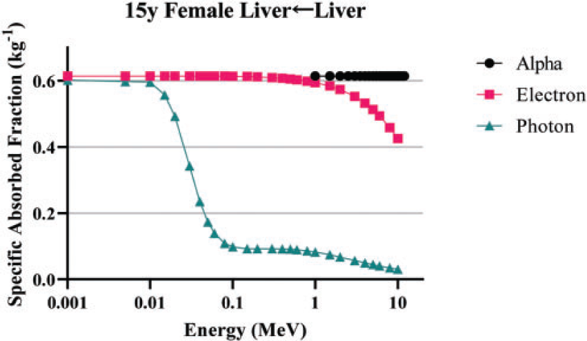
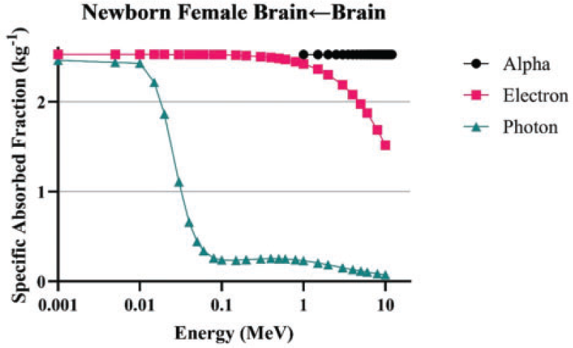
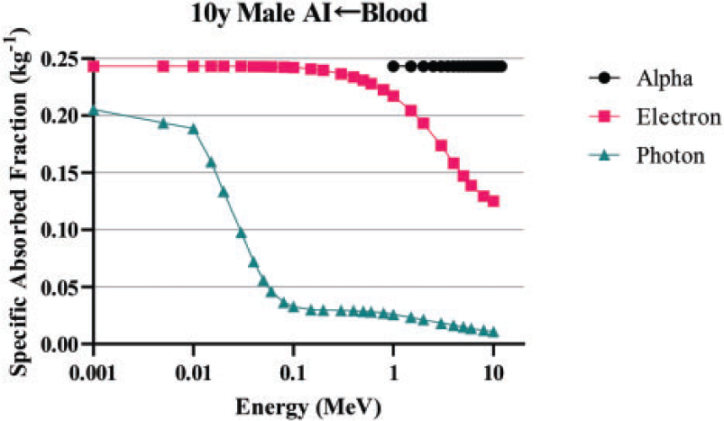
5.3.2. Age dependency

(140) Age dependency of SAFs is inversely proportional to the mass of the target when the absorbed fraction is at or near unity. This is particularly true for alpha particles and low energy electrons. Fig. 5.4 shows self-irradiation of the female breast for alpha particles, and the expected relationship between ages is observed. Fig. 5.5 shows partial self-irradiation as the right colon stem cell target comprises a portion of the right colon wall. At sufficient electron energies, the SAF drops from its low energy value and the difference between ages decreases. Fig. 5.6 shows photon self-irradiation of the skin, and displays the expected age dependency.

(141) Fig. 5.7 is an example of a result where a small inconsistency can be observed between the data for the adult and paediatric individuals. The adrenals are located in close proximity to the kidneys. At approximately 200 keV, the electron SAF for the adult begins to increase away from zero, while the SAF for younger individuals remains near zero. In the voxel phantom for the adult, the adrenals are located closer to the kidneys than in the paediatric voxel phantoms; in fact, some adrenal voxels are located adjacent to kidney voxels in the adult reference voxel phantoms. The SAF for the adult also peaks at a lower energy than it does for every other phantom, except for the newborn which is consistent with the adrenals being slightly further away in the paediatric phantoms than they are in the adult phantom. This does not necessarily indicate a problem with any of the plotted SAFs, particularly when one considers the small differences in the SAFs and the consistency of the shape amongst the individuals. It simply reflects a modelling difference which may reflect anatomical reality or biological variability.

(142) Fig. 5.8 shows SAFs for photons emitted from the cortical bone volume irradiating the thyroid. Consistency of shape is again observed, and the expected age dependency is observed.

Fig. 5.4.

Breast self-irradiation specific absorbed fractions for alpha particles in each reference female. y, years; Pub., Publication.

Fig. 5.5.

Electron self-irradiation specific absorbed fractions for the right colon stem cell target irradiated from the right colon wall in each reference male. y, years; Pub., Publication.

Fig. 5.6.

Skin self-irradiation specific absorbed fractions for photons in each reference female. y, years; Pub., Publication.

Fig. 5.7.

Specific absorbed fractions for electrons emitted from the kidneys irradiating the adrenals in each reference male. y, years; Pub., Publication.

Fig. 5.8.

Specific absorbed fractions for photons emitted from the cortical bone volume irradiating the thyroid in each reference female. y, years; Pub., Publication.

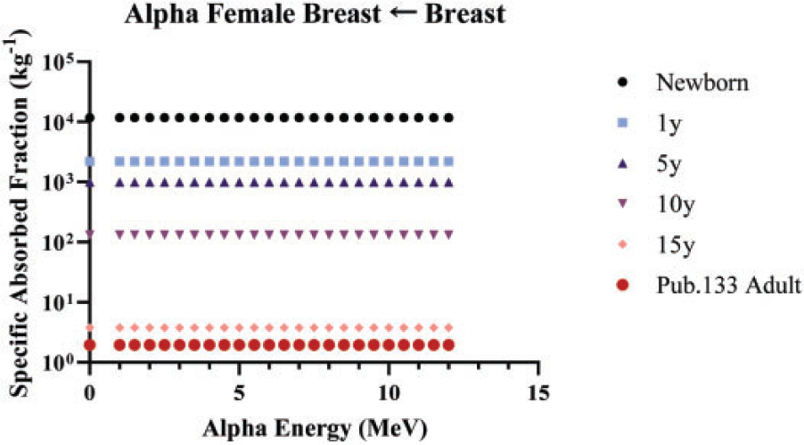
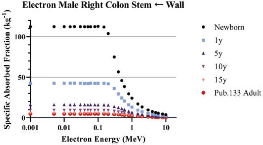
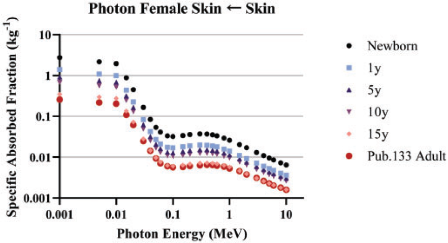
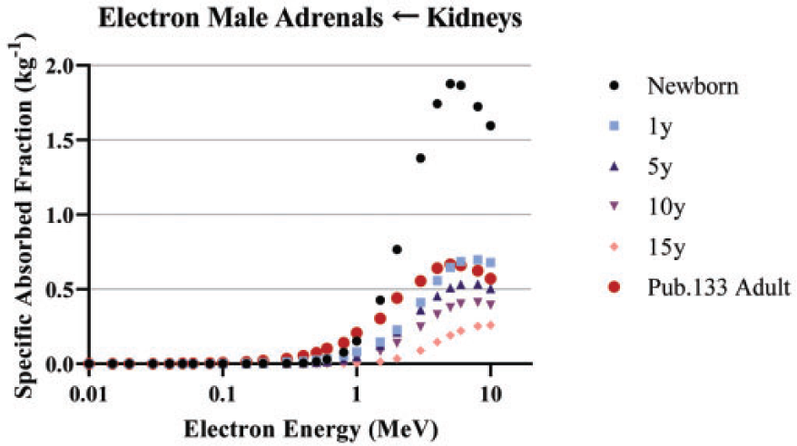
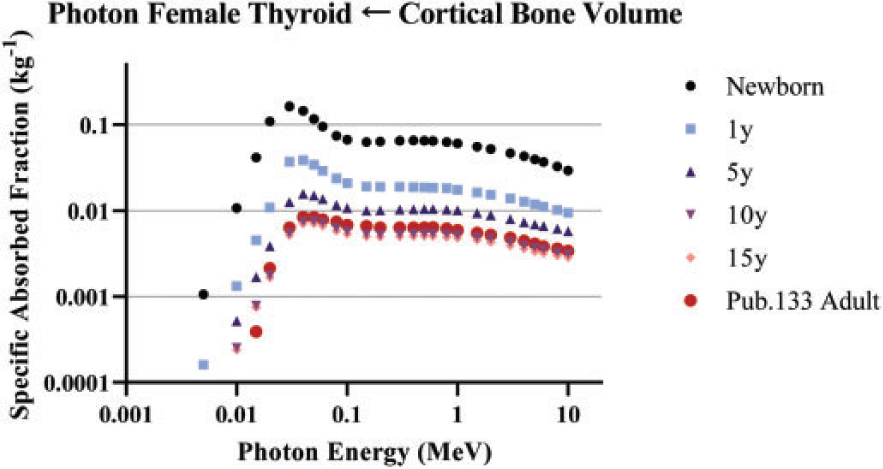
5.3.3. Geometries with relationships

(143) Fig. 5.9 shows SAFs to the newborn red marrow target for electrons emitted from a variety of skeletal source regions. At the lowest energy, SAFs approach the limiting self-irradiation values for sources in the red marrow and on the trabecular bone surface. As electron energy increases, the trabecular bone volume source is the first of the bone sources to depart from zero due to the smaller size of trabecular bone and being surrounded by marrow. Cortical bone is generally thicker and has marrow located solely on the interior side of the source region. Finally, as electron energy continues to increase, the expected convergence of the SAFs is observed. At high energies (long ranges), the medium of origin of the electron becomes irrelevant.

(144) Fig. 5.10 displays SAFs in the 15-year-old female bone endosteum target for electrons emitted from varying skeletal source regions. As the trabecular bone surface is adjacent to the bone endosteum, emissions from that surface produce the highest SAFs at low energies. The marrow source regions give non-zero low energy SAFs as the bone endosteum target consists of marrow space adjacent to the surface. Similar trends as those described in the previous paragraph are observed for intermediate and high energy electrons.

(145) Fig. 5.11 is a plot of SAFs for electrons emitted from various small intestine source regions irradiating the 10-year-old male small intestine stem cell target. The stem cell target layer is contained within the mucosa, and the mucosa is enveloped by the wall. The expected non-zero SAF is observed for both geometries, with the mucosa source producing a larger SAF due to its smaller size compared with the wall. As the villi are closer in proximity to the stem cell target than the contents, the SAF increases away from zero at a lower electron energy for emissions from the villi. Finally, as with the skeletal geometries at high energies, the SAFs converge as the location of the emission becomes less important.

(146) Fig. 5.12 is a plot of SAFs for electrons emitted from lung source regions irradiating the bronchiole secretory cell target. Source material bound in the bronchiolar epithelium overlaps with the target region, and therefore has a non-zero low energy SAF. The surface transport region is the next closest source region to the target, followed closely by material sequestered in the lamina propria, so the SAF for electrons emitted from those two regions rise away from zero at similar energies. The alveolar source region is further away, but is still in close proximity to the bronchiole target tissue. Similar to the other geometries discussed in this section, the SAFs converge at high energies.

Fig. 5.9.

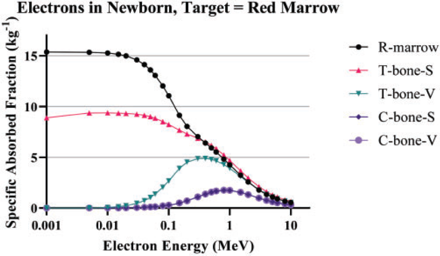
Newborn specific absorbed fractions for electrons emitted from various skeletal source regions irradiating the red marrow. R-marrow, red marrow; T-bone-S, trabecular bone surface; T-bone-V, trabecular bone volume; C-bone-S, cortical bone surface; C-bone-V, cortical bone volume.

Fig. 5.10.

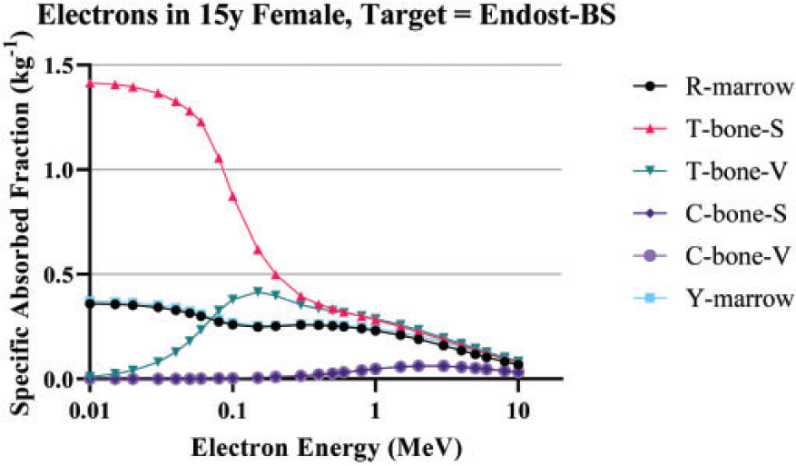
Specific absorbed fractions for 15-year-old female for electrons emitted from various skeletal source regions irradiating the bone endosteum. R-marrow, red marrow; T-bone-S, trabecular bone surface; T-bone-V, trabecular bone volume; C-bone-S, cortical bone surface; C-bone-V, cortical bone volume; Y-marrow, yellow marrow.

Fig. 5.11.

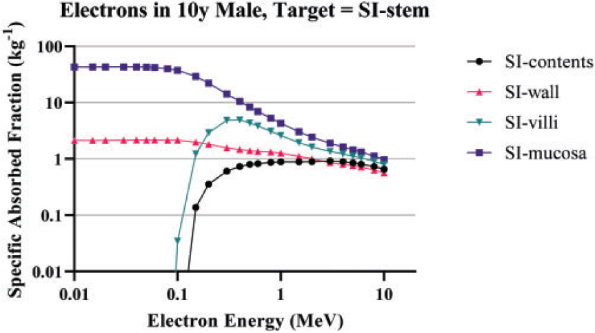
Specific absorbed fractions for 10-year-old male for electrons emitted from various small intestine (SI) source regions irradiating the small intestine stem cell (SI-stem) target.

Fig. 5.12.

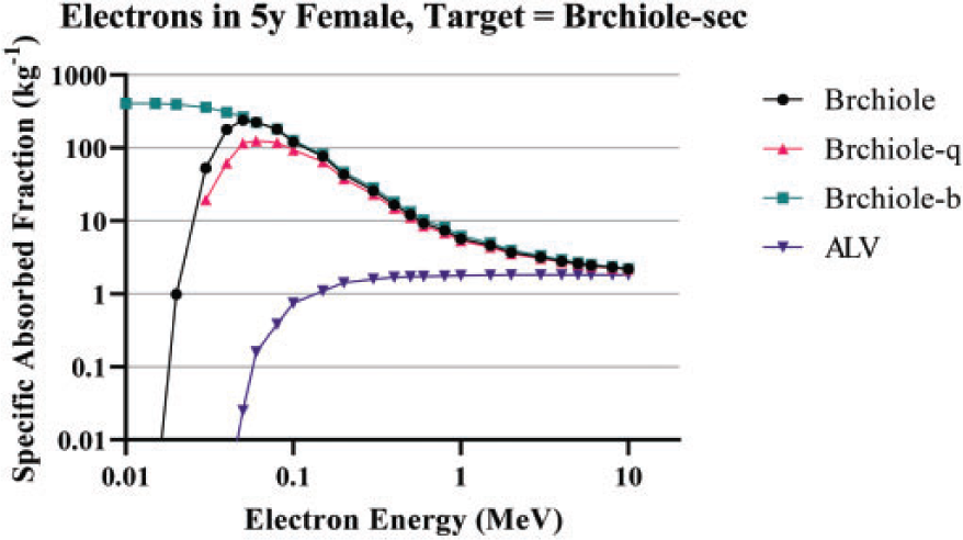
Specific absorbed fractions for 5-year-old female for electrons emitted from various lung source regions irradiating the bronchiolar secretory cell (Brchiole-sec) target. Brchiole, bronchiole surface transport region; Brchiole-q, bronchiole sequestered in lamina propria; Brchiole-b, bronchiole bound in epithelium; ALV, alveolar-interstitium.

Fig. 5.13.

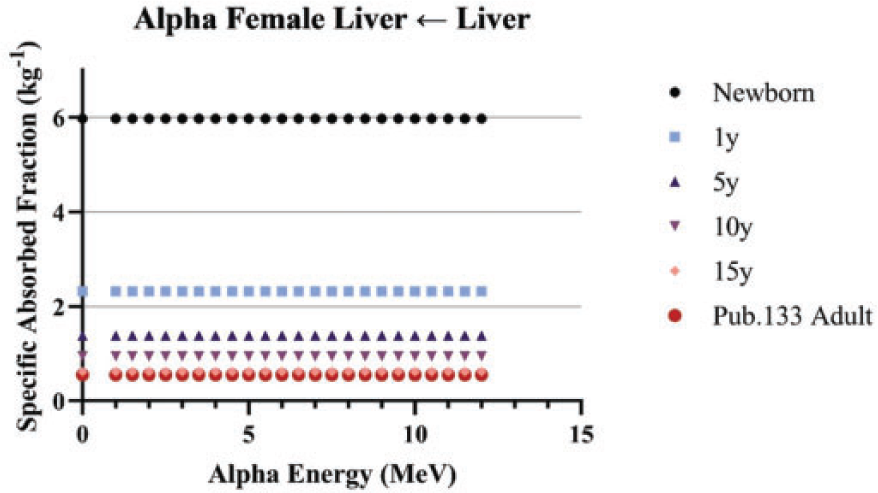
Liver self-irradiation alpha particle specific absorbed fractions in reference females y, years; Pub., Publication.

Fig. 5.14.

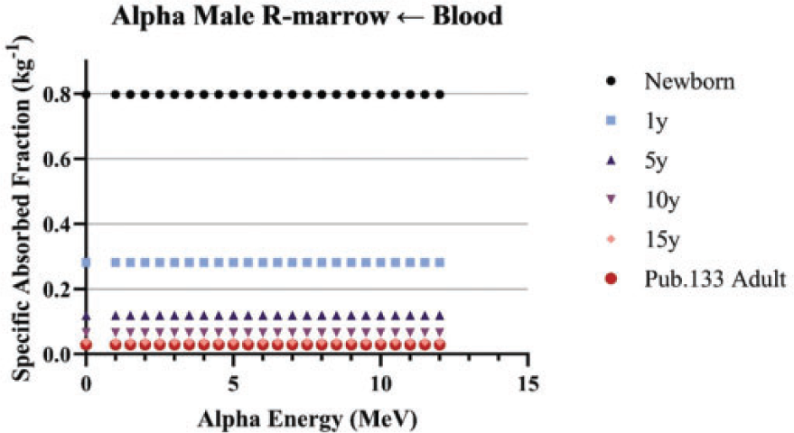
Alpha particle specific absorbed fractions to the red marrow (R-marrow) for emissions from the blood in reference males. y, years; Pub., Publication.

Fig. 5.15.

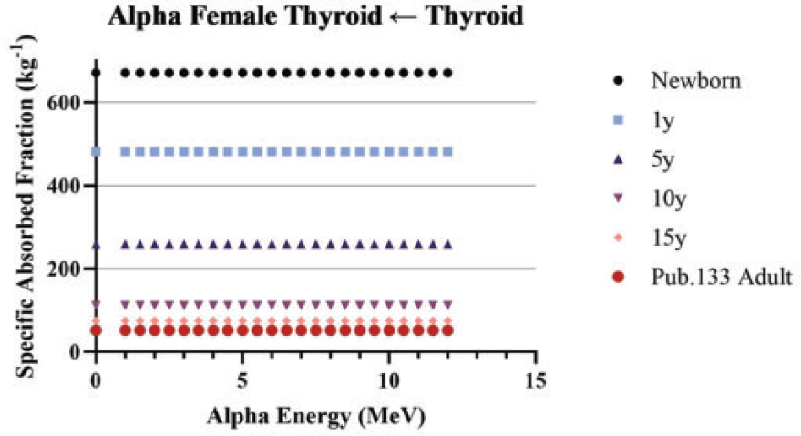
Alpha particle specific absorbed fractions for thyroid self-irradiation in reference females. y, years; Pub., Publication.

5.4. Plots of example SAFs

(147) The plots in this section contain additional examples of SAFs plotted for all reference ages. Figs 5.13–5.16 are examples of alpha particle SAFs, all of which result from absorbed fractions of unity which are independent of alpha energy. Differences, therefore, are solely the result of differences in target masses.

(148) Figs 5.17–5.20 are examples of electron SAFs. Fig. 5.17 shows electron SAFs for self-irradiation of the female breast. Fig. 5.18 shows electron SAFs in the male for irradiation of the bronchi basal target from source bound in the bronchi epithelium. Fig. 5.19 shows the irradiation of the stomach stem cell target by electrons originating in the stomach contents.

(149) Fig. 5.20 contains SAFs for electrons emitted from the blood irradiating the AI target. The expected age dependency based on varying target mass is observed. At the highest electron energies, a surprising peak is seen in the newborn SAFs. Further exploration of the source SAFs reveals that this is coming from the collisional component of the electron SAF and not the radiative component. The target in this case is the lungs, located somewhat centrally in the trunk of the body. The source is blood within the lungs (driving the SAF at low and moderate energies) and blood in tissues neighbouring the lungs. It is thought that the peak results from electrons from these neighbouring tissues (e.g. heart) being able to reach the lung target. This effect is observed in the newborn and not the older phantoms due to the smaller size and proximity of all organs in the newborn.

(150) Figs 5.21–5.24 are examples of photon SAFs. In all cases, the expected age dependency is observed.

Fig. 5.16.

Alpha particle specific absorbed fractions for salivary gland (S-gland) self-irradiation in reference males. y, years; Pub., Publication.

Fig. 5.17.

Electron specific absorbed fractions for breast self-irradiation in reference females. y, years; Pub., Publication.

Fig. 5.18.

Electron specific absorbed fractions for emissions from bronchi bound in epithelium (Bronchi-B) irradiating the bronchi basal layer (Bronchi-bas) in reference males. y, years; Pub., Publication.

Fig. 5.19.

Electron specific absorbed fractions for emissions from the stomach contents (St-cont) irradiating the stomach stem cell (St-stem) layer in reference males. y, year; Pub., Publication.

Fig. 5.20.

Electron specific absorbed fractions for emissions from the blood irradiating the alveolar-interstitium (AI) target in reference females. y, years; Pub., Publication.

Fig. 5.21.

Photon specific absorbed fractions for testes self-irradiation in reference males. y, years; Pub., Publication.

Fig. 5.22.

Photon specific absorbed fractions for ovary self-irradiation in reference females. y, years; Pub., Publication.

Fig. 5.23.

Photon specific absorbed fractions for emissions from the urinary bladder contents (UB-cont) irradiating the urinary bladder wall (UB-wall) in reference males. y, years; Pub., Publication.