
Abstract

Editorial
The Reference Computational Phantom Family
As most readers will already know, the 2007 Recommendations of the International Commission on Radiological Protection (Publication 103; ICRP, 2007) set out the foundations of the current system of radiological protection. Now 13 years old, most international guidance and many national regulations relating to radiological protection are based on Publication 103.
An important new feature in the 2007 Recommendations was a change in the way that doses from internal and external sources of ionising radiation were calculated. Previously, relatively simple mathematical models of the human body were used to calculate how energy from exposure to radiation is deposited in the various organs and tissues. With Publication 103 (ICRP, 2007), more sophisticated reference computational phantoms based on medical tomographic images replaced the simpler models.
Priority was given to developing reference computational phantoms for the adult male and female, as these are needed to calculate doses related to occupational exposure. These two phantoms, presented in Publication 110 (ICRP, 2009), are based on digitised medical image data of real people whose body height and mass were close to the reference data. The result was voxel (three-dimensional pixel) phantoms consistent with the reference anatomical and physiological parameters for males and females laid out in Publication 89 (ICRP, 2002).
The enormity of the effort and specialised skills needed to develop these phantoms may not be immediately obvious. Adjustment of the medical imaging data to match the reference parameters and a suitable posture was painstaking, as was the segmentation of the phantom into individual organs and tissues.
These reference phantoms were used to develop the dose coefficients for internal occupational exposure published in the Occupational Intakes of Radionuclides series of publications (ICRP, 2015, 2016, 2017, 2019), and the dose conversion coefficients for external exposures in Publication 116 (ICRP, 2010).
The current publication completes the reference computational phantom family, so that doses to non-adults can also be calculated. It is a large family: in addition to the two adult phantoms are 10 computational phantoms representing the Reference Male and Female at birth, 1 year, 5 years, 10 years, and 15 years of age. Like the adult phantoms, the paediatric phantoms are consistent with Publication 89 (ICRP, 2002).
Voxel phantoms were state-of-the-art in 2009, and stretched the capabilities of the computer hardware and Monte Carlo transport simulation codes available at that time. However, voxel phantoms have several important limitations. Voxels of any practicable size are unable to reproduce fine structures, some of which are important for radiological protection purposes. This includes, for example, the lens of the eye, the skin, and microstructures in bones and blood vessels. Calculation of absorbed dose to these tissues had to rely on specialised partial-body phantoms.
Like the adult phantoms, the reference paediatric phantoms also began with medical imaging data of real individuals, meticulously modified to align with reference parameters. However, the digital data were used to model the organs and tissues using mesh surfaces, capturing and adding as much fine detail as possible, based on anatomical knowledge. The results were voxelised at a very high resolution, considering the age-dependent total skin thickness, to preserve much of this detail. Today’s computer hardware and codes, enormously more powerful than those a decade ago, make it practical to use these high-resolution voxel phantoms to calculate dose coefficients. In fact, they have already been used to calculate dose coefficients for exposures to external environmental sources, to be released in the next ICRP publication (ICRP, 2020a). In addition, the Public Intake of Radionuclides series of publications, also using these high-resolution phantoms, will start to be released shortly.
This is not the end of the story. Soon it will be possible to take the next step: calculating doses using whole-body mesh phantoms directly. We are already preparing for this future. An ICRP publication on mesh-type computational phantoms is now in press (ICRP, 2020b), with the intention that these will be used as ICRP reference phantoms in the future. This will make it possible to represent the finest important structures, some just microns thick, in Monte Carlo simulations of particle transport and energy deposition.
Although mesh-type phantoms are not expected to have a significant impact on the numerical values of effective dose coefficients for everyday radiological protection purposes, other characteristics of these phantoms are attractive. Resizing mesh-type phantoms to match an individual more closely will be relatively straightforward, and the phantoms can be deformed to change posture. This could have a significant impact, for example, on the ability to assess absorbed doses to individual patients who rarely match the size and shape of the reference phantoms, and to reconstruct absorbed doses in accidental exposures where postures may also be an important consideration.
The paediatric reference computational phantoms in this publication mark an important shift from purely voxel-based phantoms to a hybrid format developed using anatomical data from medical scans and knowledge of fine anatomical structures, resulting in voxel phantoms of arbitrarily high resolution.
References
Christopher H. Clement
Editor-In-Chief
Paediatric Reference Computational Phantoms
ICRP PUBLICATION 143
Approved by the Commission in May 2019
Section 1 summarises the main reasons for constructing these phantoms – voxel phantoms that comply with the reference anatomical characteristics of the non-adult reference individuals presented in ICRP Publication 89. Section 2 reviews the body size/shape and organ-specific specifications of the ICRP paediatric reference phantoms. Section 3 presents, in detail, the methods of their construction, which includes nine steps in their development: (1) selection of computed tomographic (CT) data; (2) segmentation of those CT images; (3) body contour and organ modelling via non-uniform rational basis spline (NURBS)/polygon mesh (PM) surfaces; (4) adjustments of outer body contour to match total body mass; (5) adjustments of individual organ values to match reference masses; (6) subdivision of the skeletal tissues; (7) voxelisation of the NURBS/PM surfaces; (8) voxel retagging for lymphatic nodes and skeletal muscle; and (9) further modifications to bring the series of paediatric phantoms into a structure identical to that originally established for the adult phantoms of ICRP Publication 110. Section 4 follows with a description of the ICRP paediatric reference phantoms, including their main characteristics, skeletal source/target regions, regional blood distribution, and phantom limitations.
The publication is supported by a series of annexes. Annex A provides details on tissue ID numbers, tissue media, mass densities, and organ locations by both coordinate position and voxel count. Annex B provides a complete list of the various age-dependent and gender-dependent tissue media, their phantom masses, and elemental compositions. Annexes C and D provide a listing of all source and target regions, respectively, needed for internal as well as external dosimetric applications. Annexes E and F provide depth distributions and organ pair distance distributions, respectively, in a manner similar to that provided in ICRP Publication 110 for the adult phantoms. Annex G provides cross-sectional images – sagittal, coronal, and transverse planes. Finally, Annex H gives a description of the electronic files available for download and use of each of the 10 paediatric reference computational phantoms.
© 2020 ICRP. Published by SAGE.
Keywords:: Computational phantoms, Voxel models, Paediatric reference individuals
1. INTRODUCTION
(1) In 2009, the International Commission on Radiological Protection (ICRP) issued Publication 110 which described the development and subsequent adoption of two computational voxel phantoms representing the reference adult male and reference adult female (ICRP, 2009). These phantoms were based on medical image data of real people and were consistent with the information given in Publication 89 on the reference adult anatomical and physiological parameters (ICRP, 2002). The reference voxel phantoms were constructed following modification of previously existing voxel models (Golem and Laura) of two individuals whose body height and mass closely resembled the reference data. Internal organ masses of both models were subsequently adjusted to the ICRP data on the reference adult male and reference adult female, without significant alterations to their realistic anatomy. Publication 110 describes the methods used for this process and the characteristics of the resulting voxel phantoms. (2) Since their development and adoption by the Commission, the Publication 110 (ICRP, 2009) adult reference phantoms have been used in a number of task group activities within ICRP Committee 2. In 2010, the Commission issued Publication 116 reporting dose coefficients for both organ equivalent dose and effective dose following occupational exposures to externally incident fields of photons, electrons, positrons, neutrons, and helium ions (ICRP, 2010). This publication represented the first use of the new reference adult voxel phantoms by Committee 2. The Publication 110 (ICRP, 2009) phantoms were also used to construct external dose coefficients relevant to both cosmic ray exposures (ICRU, 2010) and the radiation fields in the space environment (ICRP, 2013). In Publication 133, the Commission reported adult reference specific absorbed fraction (SAF) values for internally emitted photons, electrons, alpha particles, and neutrons (the latter associated with internal emitters decaying via spontaneous fission) (ICRP, 2016a). These adult SAF values were then used in the computation of dose coefficients of both equivalent organ dose and effective dose following both ingestion and inhalation of radionuclides in occupational settings as described in Publication 130 [Occupational Intakes of Radionuclides (OIR) Part 1] (ICRP, 2015). Dose coefficients for internal exposures of the reference adults are given in the OIR series which presently includes Publication 134 (OIR Part 2) (ICRP, 2016b), Publication 137 (OIR Part 3) (ICRP, 2017), and Publication 141 (OIR Part 4) (ICRP, 2019). (3) The current publication extends the series of ICRP reference phantoms to include male and female reference newborn, 1-year-old, 5-year-old, 10-year-old, and 15-year-old phantoms. These paediatric reference phantoms are presently being used in two series of Committee 2 activities. The first is the establishment of organ and effective dose coefficients for environmentally localised radionuclides to include air submersion, water immersion, and ground exposure. In this task group activity, the Publication 110 (ICRP, 2009) adult phantoms are used, as well as the paediatric reference phantoms of the present publication. The second activity is the development of updated dose coefficients for environmental intakes of radionuclides (ingestion and inhalation) to include all members of the general public – reference adults, adolescents, and children. An extension of Publication 133 (ICRP, 2016a) describing photon, electron, alpha particle, and internal neutron SAF values in the ICRP paediatric phantom series is presently under development.
2. SPECIFICATIONS OF THE ICRP PAEDIATRIC REFERENCE PHANTOMS
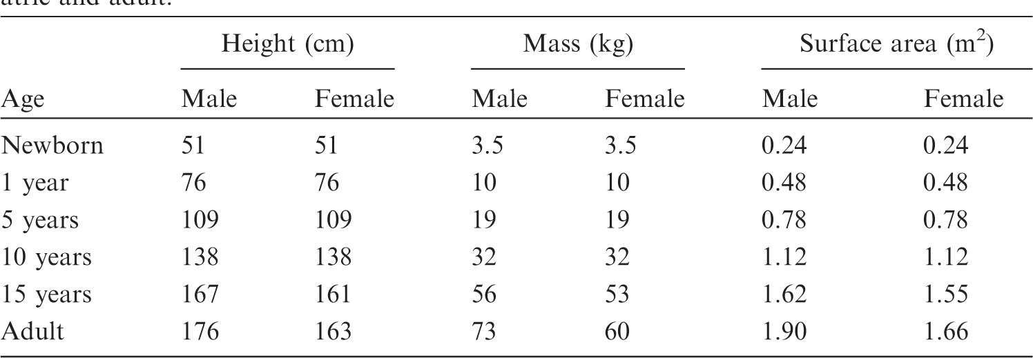
(4) The voxel phantoms used for calculation of energy deposition in body organs and tissues (target regions) following the 2007 Recommendations (ICRP, 2007) should accommodate all organs and tissues that are relevant to the assessment of human exposure to ionising radiation for radiological protection purposes. These target regions include: active bone marrow, adrenal glands, brain, breast, colon, endosteal tissues of the skeleton, extrathoracic (ET) airways, lens of the eye, gallbladder, heart, kidneys, liver, lungs, lymphatic nodes, skeletal muscle, oesophagus, oral mucosa, ovaries, pancreas, prostate gland, salivary glands, skin, small intestine, spleen, stomach, testes, thymus, urinary bladder, and uterus. Furthermore, additional target regions have been identified within the Human Respiratory Tract Model and Human Alimentary Tract Model. These target regions include: alveolar-interstitium, basal cells of anterior and posterior nasal passages and pharynx, basal cells of bronchi, lymph nodes of ET and thoracic regions, secretory cells of bronchi and bronchioles, and tongue and tonsils. (5) When radioactive material is incorporated into the body, those organs, tissues, and body regions where radionuclides reside or pass through become source regions that irradiate other (target) regions. Many regions are both source and target regions. Additional source regions are located in the alimentary and respiratory tracts, as well as in the skeleton. Certain individual anatomical regions have to be considered differently depending on the rate with which the material passes through or is cleared from them. These additional source regions include: oral cavity, teeth surfaces, teeth volumes, oesophagus (fast, slow), stomach contents, small intestine contents, right colon (contents, wall), left colon (contents, wall), rectosigmoid colon (contents, wall), gallbladder contents, urinary bladder contents, nasal passages (anterior and posterior surfaces), pharynx, sequestered ET2 region, bronchi (fast, slow, bound, sequestered), bronchioles (fast, slow, bound, sequestered), blood vessels (head, trunk, legs, arms), cortical bone (surface, volume), trabecular bone (surface, volume), and inactive bone marrow. To support applications to the kidney dosimetry in nuclide medicine, the models of the kidneys in the reference paediatric phantoms include separate regions for the renal cortex, renal medulla, and renal pelvis. As was done for the adult reference phantoms of Publication 110 (ICRP, 2009), the skeletal tissues of the reference paediatric phantoms are given as regions of cortical bone, spongiosa, and medullary marrow. Voxel regions of spongiosa thus represent a homogenous mixture of trabecular bone, active bone marrow, and inactive bone marrow, whose mass fractions vary with skeletal bone location and phantom age and, for the 15-year-old, sex. (6) The body morphometry specifications of the ICRP paediatric reference individuals are given in Table 2.1 as reported in Table 2.9 of Publication 89 (ICRP, 2002). The specifications of reference body size and shape are thus limited to total body mass and standing height. Body surface area is also specified, but the reference values given in Table 2.1 derive from the expression reported in Gehan and George (1970) whose input is standing height and body mass; thus, body surface area is not an independent parameter for phantom construction. Reference values of organ mass are further given in Table 2.8 of Publication 89 for the full series of 12 reference individuals – male and female newborns, 1-year-olds, 5-year-olds, 10-year-olds, 15-year-olds, and adults. For the reference newborn, 1-year-old, 5-year-old, and 10-year-old, reference values of standing height and total body mass are shown to be equivalent for both the male and female. This feature of the paediatric reference individuals – equivalent body size of the male and female at each reference age – also extends to reference organ masses. The few exceptions are noted in Table 2.8 of Publication 89 and include different male and female brain masses at 5 and 10 years of age, and different male and female thymus masses at 10 years of age.
1
For the 15-year-old male and female, Publication 89 indicates distinctive reference values for organ masses, standing heights, and total body masses. These features of uniformity of male and female reference individuals at ages below 15 years were utilised in the development of the corresponding reference phantoms such that computed tomography (CT) images of only one sex were selected as the source anatomy for phantom construction. (7) A list of all organs, tissues, and regions that were defined in the paediatric reference phantom series, and have been assigned an individual organ identification (ID) number, is given in Annex A. Annex B gives a list of different tissue types of which the organs and tissues consist, along with their elemental compositions. Annex C presents a list of all source organs and regions, together with the organ ID numbers by which they are represented. Annex D gives the same information for target organs and tissues.
Reference values for standing height, body mass, and total body surface area of the International Commission on Radiological Protection reference individuals – both paediatric and adult.
3. DEVELOPMENT OF THE ICRP PAEDIATRIC REFERENCE PHANTOMS
(8) The paediatric reference computational phantoms of this publication were derived from a corresponding series of computational phantoms developed at the University of Florida (UF) and later at the US National Cancer Institute (NCI) (Lee et al., 2010). This section reviews: (1) the source of CT data for UF/NCI phantom construction; (2) the techniques applied to create the UF/NCI phantoms consistent with the anatomic specifications of Publication 89 (ICRP, 2002) and other morphometric data; and (3) modifications applied to the UF/NCI phantoms to bring them into a format consistent with that of the adult male and female reference computational phantoms of Publication 110 (ICRP, 2009).
3.1. Overview of the paediatric phantom construction methodology
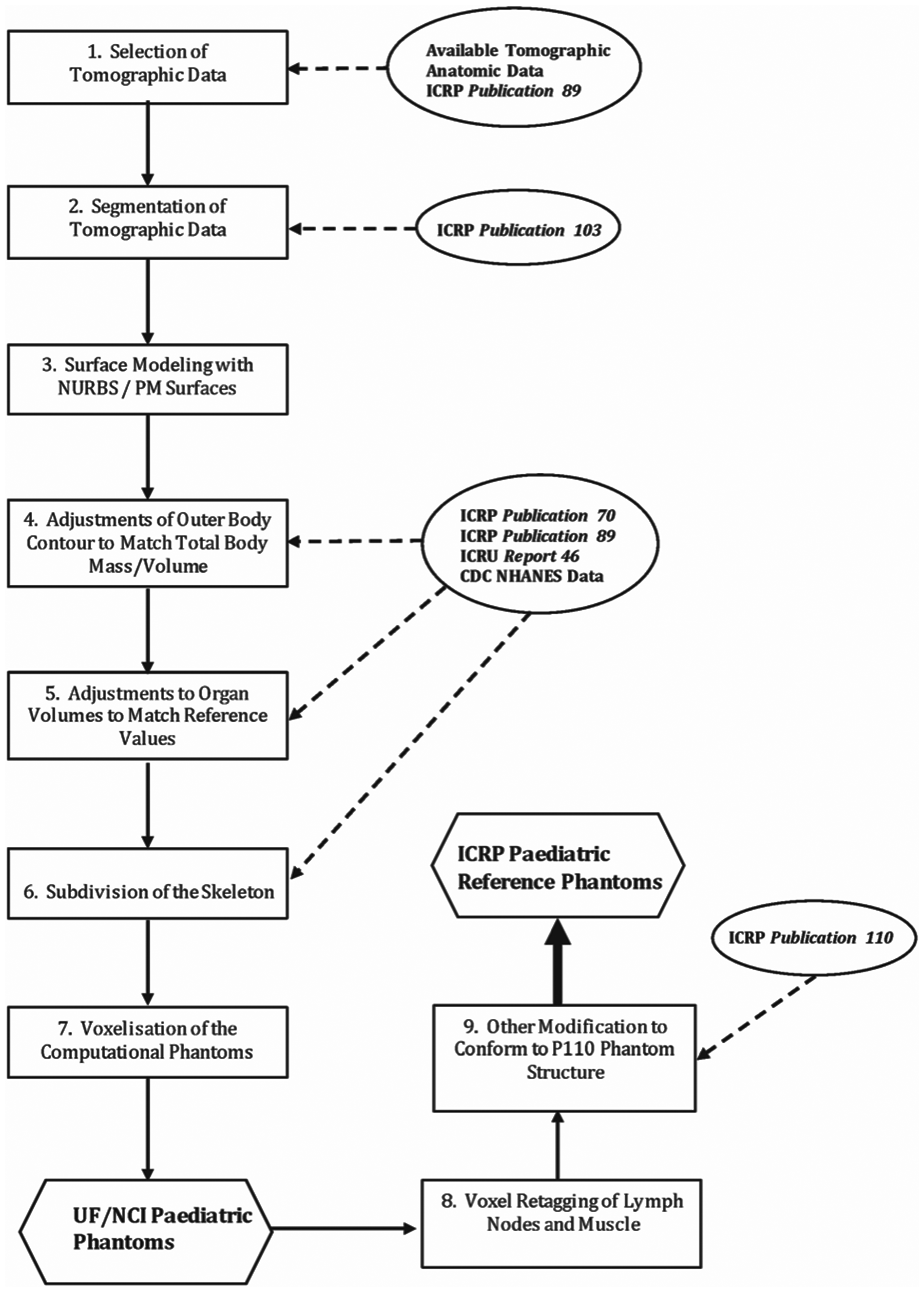
(9) The process by which the paediatric reference phantoms were constructed is outlined in schematic form in Fig. 3.1. Step 1 involved the selection of CT data for phantom construction, followed by manual segmentation of that data for identification of individual organs and tissues in Step 2. This second step effectively results in a traditional voxel phantom derived from the source CT image set. In the present work, however, an additional step – Step 3 – was employed whereby the voxelised surfaces of the outer body contour and all internal organs were modelled using non-uniform rational basis spline (NURBS) and polygon mesh (PM) surfaces to smooth them in a three-dimensional manner. A further advantage of this approach was that targeted organ volumes could be readily achieved through adjusting the NURBS or PM surfaces normally outward or inward, in contrast to the process employed in Publication 110 (ICRP, 2009) which required the removal or addition of individual layers of voxels to decrease or increase, respectively, a given organ volume. Steps 4 and 5 thus allowed modelling of reference body morphometry and reference internal organ volumes, respectively. Step 6 resulted in conversion of a homogeneous model of the skeletal bones to models which have separate regions of cortical bone, trabecular spongiosa, and medullary marrow. At the time of their development, radiation transport codes did not yet have the capability to transport radiation particles directly within the NURBS/PM structure, and so Step 7 included voxelisation – a process by which voxels are inserted interior to the PM or NURBS surfaces of body and body organs [see further description given in Lee et al. (2010)]. The advantage here, however, is that the voxel size applied in Step 7 is user-defined and not limited to the voxel dimensions of the original CT image set. The final step – Step 8 – involved retagging of voxels to provide a model of the skin, lymphatic nodes, and skeletal muscle. Step 9, the final activity of phantom development, included further modifications of these reference voxel phantoms to bring them into full compliance with the phantom structure of Publication 110. These steps are further described below. Schematic for constructing the paediatric series of male and female computational reference phantoms. UF, University of Florida; NCI, US National Cancer Institute; P110, ICRP Publication 110.
3.2. Source tomographic data for paediatric reference phantom construction (Step 1)
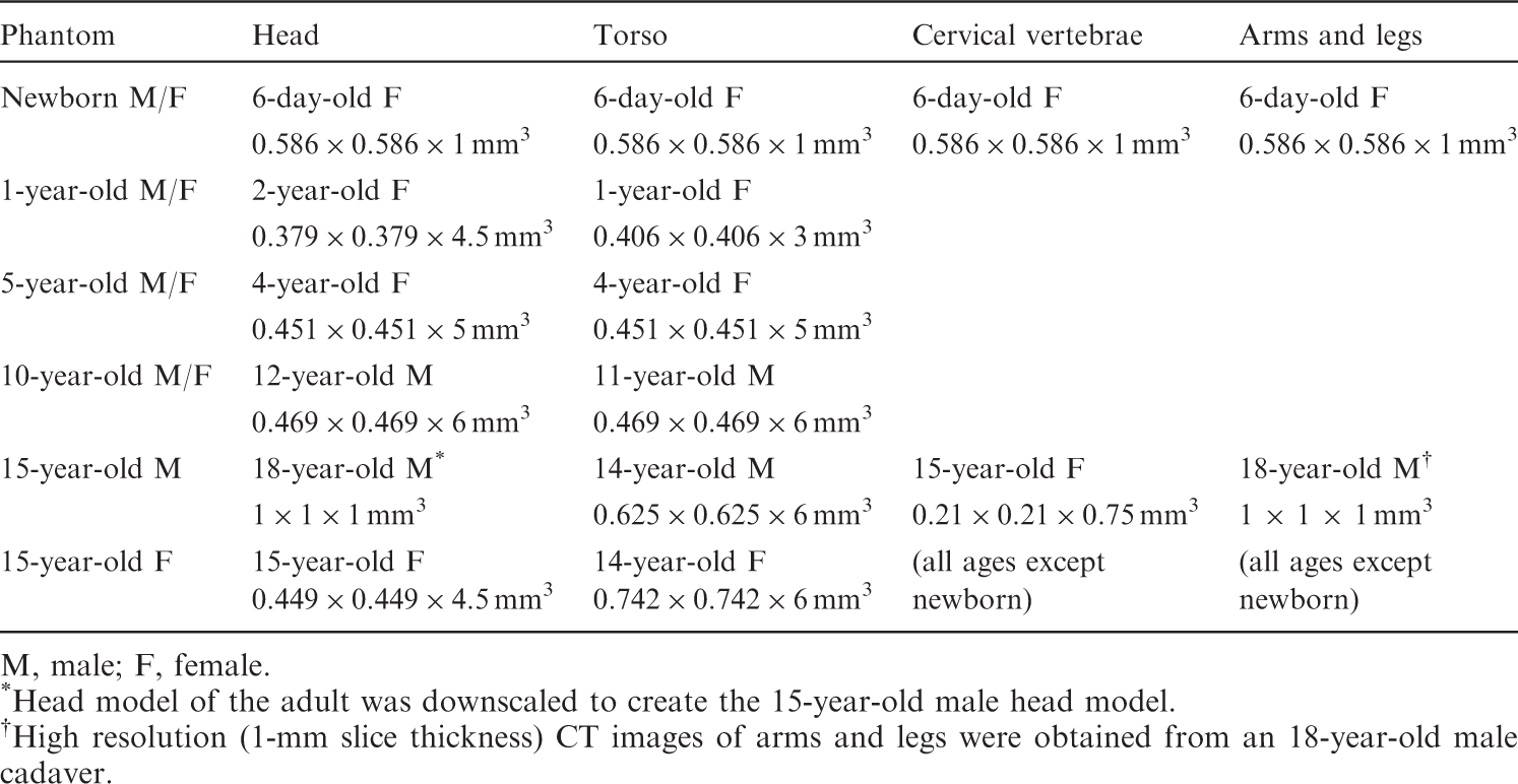
(10) CT image data used for phantom construction are summarised in Table 3.1. CT images for phantom construction came from one of two sources: (1) prospective images of cadavers (newborn model); or (2) retrospective review and image retrieval from radiology archives at the UF Health Children’s Hospital (all other reference ages). Prior to final adoption for phantom construction, CT images were reviewed by the Chief of Paediatric Radiology at UF for any gross abnormalities which would preclude them from representing ‘normal’ paediatric anatomy. While CT images of male and female patients were used in the construction of 15-year-old male and female reference phantoms, respectively, images from only one gender were used as source data for the construction of the newborn (female data), 1-year-old (female data), 5-year-old (female data), and 10-year-old (male data) reference phantoms. At each reference age, the phantom of the opposite sex was thus created via removal and re-insertion of the appropriate sex organs in their NURBS/PM format (see Section 3.3). (11) Development of the male and female newborn reference phantoms is described in Nipper et al. (2002) and Lee et al. (2007). CT source data for their construction consisted of 485 CT images of a 6-day-old female cadaver. The patient died in an attempt to correct congenital abnormalities of the great vessels, and was imaged within 24 h of death. The imaging data were contiguous with no gaps or data overlaps. Each slice was saved as a 512 × 512 image with an in-plane pixel resolution of 0.586 mm × 0.586 mm and a slice thickness of 1 mm. The cadaver mass had been recorded at 3.83 kg at the time of death. (12) Development of the male and female reference phantoms at 1, 5, and 10 years of age is described in Lee et al. (2010). The 1-year-old reference phantoms were created based upon head CT images of a 2-year-old female (3.79 × 0.379 × 4.5 mm3 resolution) and chest–abdomen–pelvis (CAP) images of a 1-year-old female (0.406 × 0.406 × 3 mm3 resolution). The 5-year-old reference phantoms were created based upon head and CAP CT images of the same patient – a 4-year-old female (0.451 × 0.451 × 5 mm3 resolution). The 10-year-old reference phantoms were created based upon head CT images of a 12-year-old male and CAP images of an 11-year-old male (both at 0.469 × 0.469 × 6 mm3 resolution). For each phantom, two supplemental image sources were also applied to phantom construction. These included higher-resolution CT images of the cervical spine of a 15-year-old female (0.210 × 0.210 × 0.75 mm3) and CT images of the arms and legs of an 18-year-old male cadaver (1 × 1 × 1 mm3 resolution). Both the cervical spine, arm, and leg models were proportionally scaled to target reference body morphometry data as described below. (13) Development of the male and female 15-year-old reference phantoms is described in Lee et al. (2008). The 15-year-old male reference phantom was based upon head CT images of an 18-year-old male (1 × 1 × 1 mm3 resolution) and CAP CT images of a 14-year-old male (0.625 × 0.625 × 6 mm3 resolution). The 15-year-old female reference phantom was based upon head CT images of a 15-year-old female (0.449 × 0.449 × 4.5 mm3) and CAP CT images of a 14-year-old female (0.742 × 0.742 × 6 mm3).
3.3. Construction of the paediatric reference phantom series (Steps 2–5)
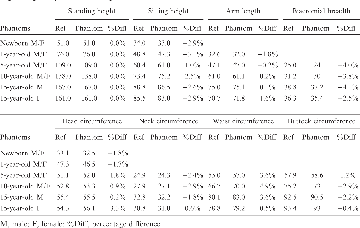
(14) CT images from all data sets of Table 3.1 were imported into the three-dimensional image segmentation software 3D-Doctor where organs and tissues were segmented and later imported into the NURBS modelling tool Rhinoceros 4.0. As described in Lee et al. (2010), most organs and tissues were modelled as NURBS surfaces with the exclusion of the skeleton, brain, and ET airways which could be modelled more effectively as PM surfaces. (15) Once provisional organ and tissue models were developed via NURBS and PM surfaces, the phantom body dimensions were matched to anthropometric data from several literature sources as summarised in Table 3.2 under Step 3. A total of eight reference anthropometric parameters were employed: height (both standing and sitting), length (total arm), biacromial breadth,
2
and circumference (head, neck, waist, and buttocks). Of these, Publication 89 (ICRP, 2002) provides reference values for standing height alone. Sitting heights for 5-year-old and 10-year-old children, head circumferences for 1-year-old and 5-year-old children, buttock circumferences for 5-year-old and 10-year-old children, and biacromial breadths for 5-year-old and 10-year-old children were obtained from the National Health and Nutrition Examination Survey (NHANES) III (1988–1994) data series,
3
while other anthropometric data were provided by the database Anthrokids compiled by the US Consumer Product Safety Commission.
4
Waist circumferences for 5-year-old and 10-year-old children were obtained from the NHANES IV (1999–2002) survey. As a result, only four parameters (standing and sitting height, arm length, and head circumference) were available for the 1-year-old phantoms, and only three parameters (standing and sitting height, and head circumference) were available for the newborn phantoms. At each age below 15 years, these same parameters were used for both the male and female phantoms. Once body dimensions were matched to standard anthropometric data, the organ and tissue volumes were adjusted to match reference organ masses provided in Publication 89 to within a tolerance of 1% under Step 4. Targeted organ volumes were taken as ratios of the reference mass and reference tissue densities taken from ICRU Report 46 (ICRU, 1992). (16) Reference lengths and masses for the walls of the alimentary tract organs (oesophagus, small intestine, right colon, left colon, and rectosigmoid colon) are available from Publications 89 and 100 (ICRP, 2002, 2006), whereas reference wall thickness is not reported. As stated in Section 6.3.10 of Publication 89, the reference lengths are physiological lengths representing those measured in a living person. The values are usually less than corresponding anatomical lengths measured at autopsy or during surgical tissue removal. In this study, the lengths of the alimentary tract organs were matched to their ICRP reference values to within a tolerance of 5% by adjusting the length of the central trace of each segment, which in turn was obtained from the original patient CT images. Second, a NURBS pipe model with an appropriate radius was generated along these central tracks via a trial and error process until a realistic shape and curvature was obtained. The alimentary tract wall masses were then matched to the reference masses given in Publication 89 to within a tolerance of 1%. (17) The skin thicknesses (epidermis plus dermis) were derived from three different reference parameters: (1) skin mass and (2) body surface area provided in Sections 2.3.1 and 10.4 of Publication 89, respectively; and (3) reference skin density from ICRU Report 46 (ICRU, 1992). Reference skin volumes were first calculated from reference skin masses and tissue densities. Next, a derived skin thickness was taken as the ratio of the reference skin volume and associated surface area. This approach, however, yielded a sharp discontinuity in skin thicknesses between the 10-year-old and 15-year-old phantoms. In the original pulsed ultrasound study by Tan et al. (1982) cited in Publication 89 (ICRP, 2002), however, these authors concluded that ‘skin thickness was found to increase linearly with age up to the age of 20 years’. Consequently, adjustments were made to these derived thicknesses at 5 and 10 years of age to provide for a more continuous change in skin thickness with increasing phantom age.
3.4. Skeletal tissue model of the paediatric reference phantom series (Step 6)
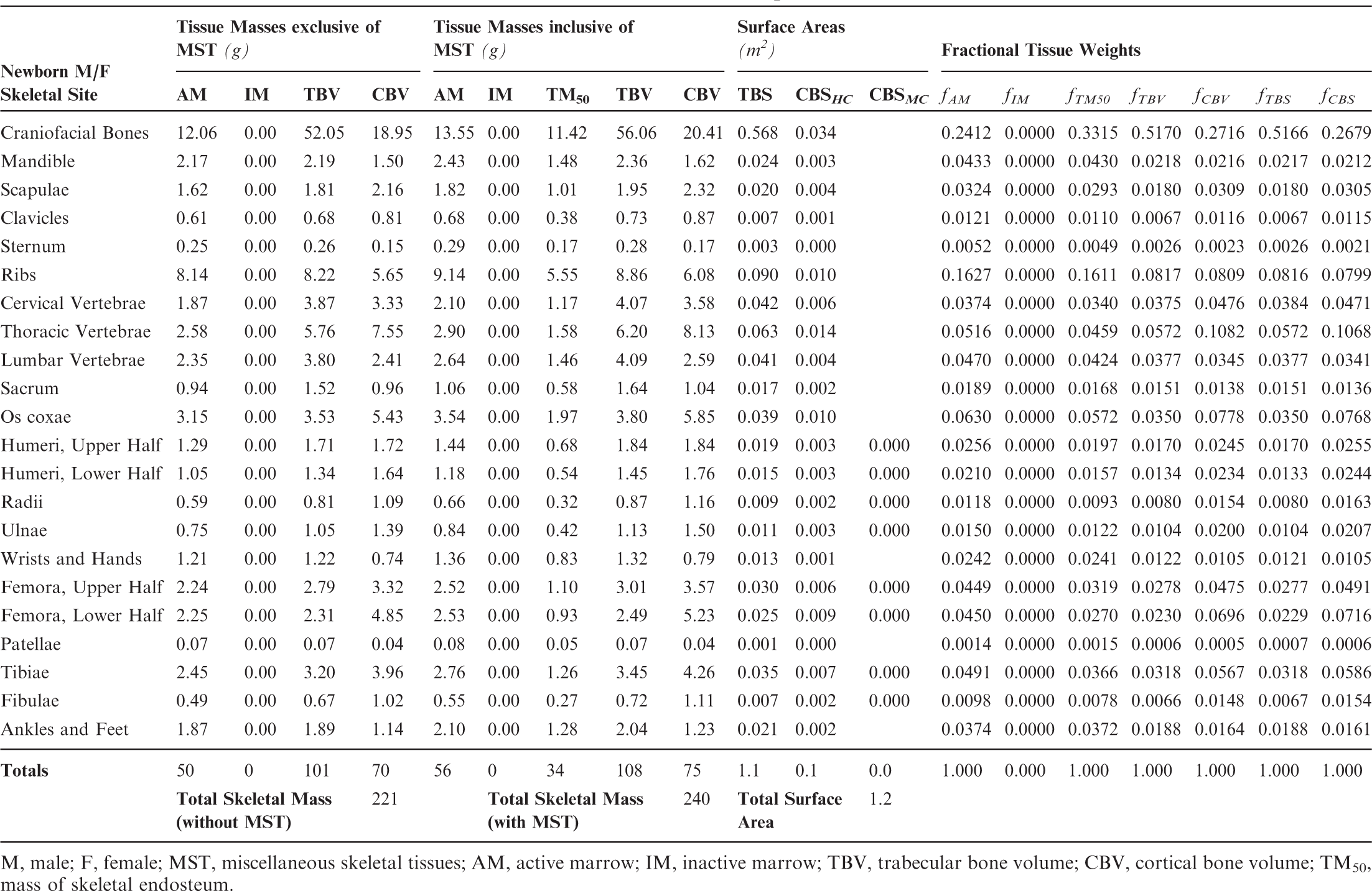
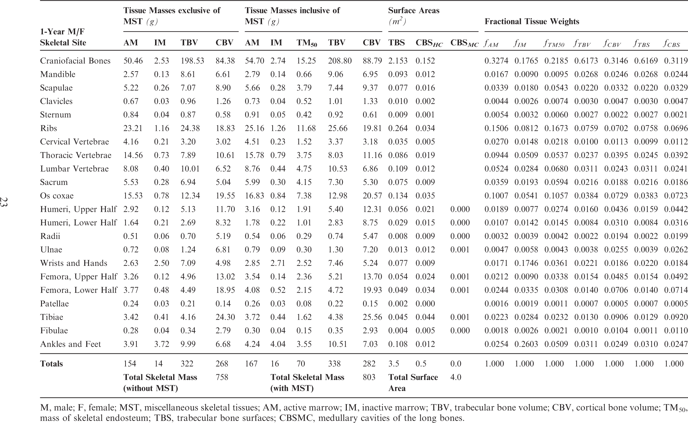
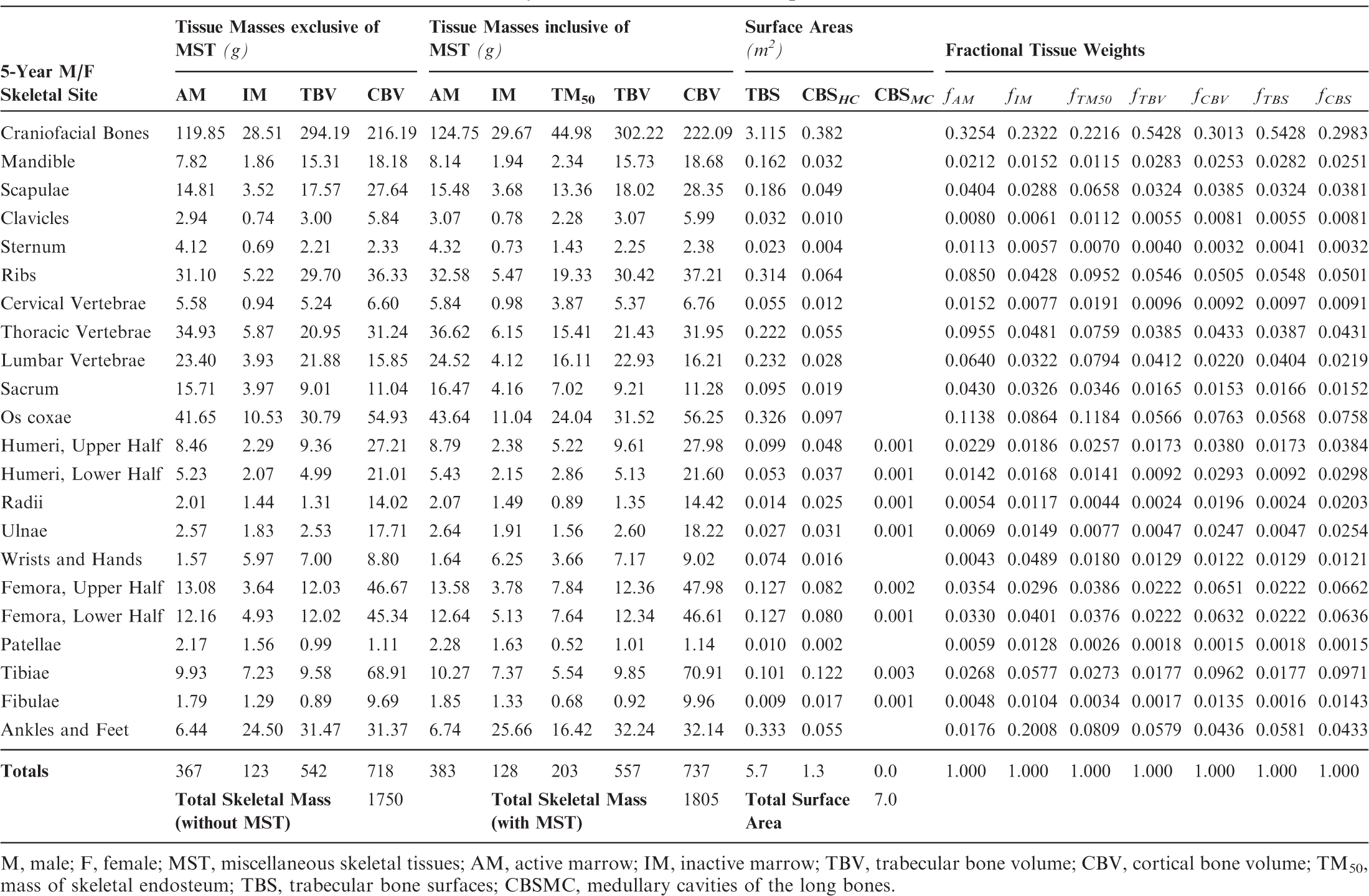
(18) The skeletal tissues within the UF/NCI paediatric phantom series originally described by Lee et al. (2010) presented the skeleton as a homogeneous mixture of mineral bone (cortical and trabecular) and marrow tissues (active and inactive). As described in Pafundi (2009), a further effort was undertaken to develop an age-dependent and bone-specific skeletal tissue model consistent in structure to that of the ICRP adult reference phantoms of Publication 110 (ICRP, 2009). This step included the creation of additional PM surfaces to separately define regions of cortical bone, trabecular spongiosa, and the medullary cavities of the long bones. (19) The tissue models were developed using the following criteria. First, the volumes available to assign the various tissue elements were defined by the homogeneous bone volumes present within the constructed age-dependent phantom series which were set at reference heights. Second, the partitioning of mineral bone into cortical bone and trabecular bone was allowed to vary with age based upon the finding by Pafundi et al. (2009) that while cortical bone accounts for 79% of total mineral bone in the 15-year-old phantom, it only accounts for 41% of total mineral bone in the newborn phantom (Pafundi et al., 2009, 2010). For each computational phantom, reference values for total mineral bone were targeted, and not those for cortical and trabecular bone separately. As a result, only the 15-year-old phantoms approached a skeletal average ratio of 80% cortical bone and 20% trabecular bone as given in Publication 89 (ICRP, 2002) for the reference adult. Third, marrow cellularity was assigned to its reference values given in Publication 70 (ICRP, 1995) at each bone site and at each reference age. Reference values for total marrow, and not active and inactive marrow individually, were assigned across the paediatric skeleton at each reference age. (20) Tables 3.3–3.8 detail the skeletal tissue models for each of the paediatric reference phantoms. Tissue masses are given for active marrow (AM), inactive marrow (IM), trabecular bone volume (TBV), and cortical bone volume (CBV), both with and without the addition of miscellaneous skeletal tissues (MST). Masses of skeletal endosteum (TM50) are also given, based in part on microCT image analysis as described in Pafundi (2009). Tables 3.3–3.8 next provide values of trabecular bone surfaces (TBS) and cortical bone surfaces (CBS). Values of CBS are further given for those along the Harversian canals of cortical bone (CBSHC) and those along the medullary cavities of the long bones (CBSMC). Fractional tissue weights are given for AM, IM, TM50, TBV, CBV, TBS, and CBS as needed for simulating source emissions within the skeletal tissues. Computed tomography (CT) image sources employed in the development of the University of Florida/US National Cancer Institute paediatric reference phantoms. M, male; F, female. Head model of the adult was downscaled to create the 15-year-old male head model. High resolution (1-mm slice thickness) CT images of arms and legs were obtained from an 18-year-old male cadaver. Comparison of reference and phantom values (cm) for morphometric parameters regarding body size and shape. M, male; F, female; %Diff, percentage difference. Skeletal tissue model for the reference newborn male and female phantoms. M, male; F, female; MST, miscellaneous skeletal tissues; AM, active marrow; IM, inactive marrow; TBV, trabecular bone volume; CBV, cortical bone volume; TM50, mass of skeletal endosteum. Skeletal tissue model for the reference 1-year-old male and female phantoms. M, male; F, female; MST, miscellaneous skeletal tissues; AM, active marrow; IM, inactive marrow; TBV, trabecular bone volume; CBV, cortical bone volume; TM50, mass of skeletal endosteum; TBS, trabecular bone surfaces; CBSMC, medullary cavities of the long bones. Skeletal tissue model for the reference 5-year-old male and female phantoms. M, male; F, female; MST, miscellaneous skeletal tissues; AM, active marrow; IM, inactive marrow; TBV, trabecular bone volume; CBV, cortical bone volume; TM50, mass of skeletal endosteum; TBS, trabecular bone surfaces; CBSMC, medullary cavities of the long bones.
3.5. Phantom voxelisation (Step 7)
(21) At the time of their development, radiation transport codes required that complex anatomical models of the human body be presented in the form of an array of voxelised tissue elements. Resultantly, Step 7 in the development of the ICRP paediatric reference phantoms involved the placement of arrays of tagged tissue voxels within the NURBS/PM surfaces of all internal organs as well as within the surface of the outer body contour. This process – termed ‘voxelisation’ – was performed using an in-house routine coded in MATLAB as described previously in Lee et al. (2007) for the newborn phantom, and then later in Lee et al. (2010) for the UF/NCI phantom series. Targets for voxel shape (cubic or parallelepiped) were driven by considerations of the age-dependent total reference skin thickness, while the targeted total voxel matrix size was set at approximately 55 million voxels (see Section 4.1).
3.6. Modifications to the paediatric reference phantom series (Steps 8 and 9)
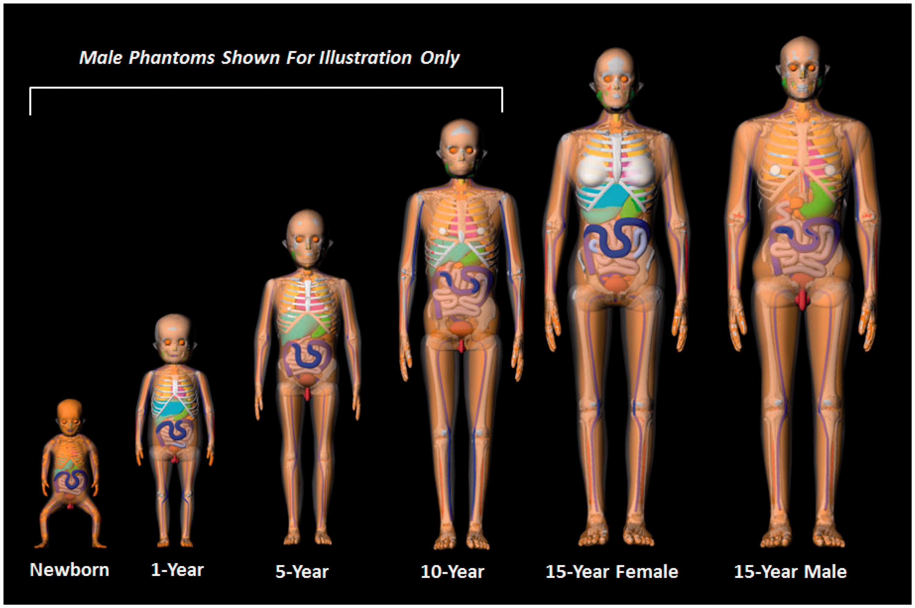
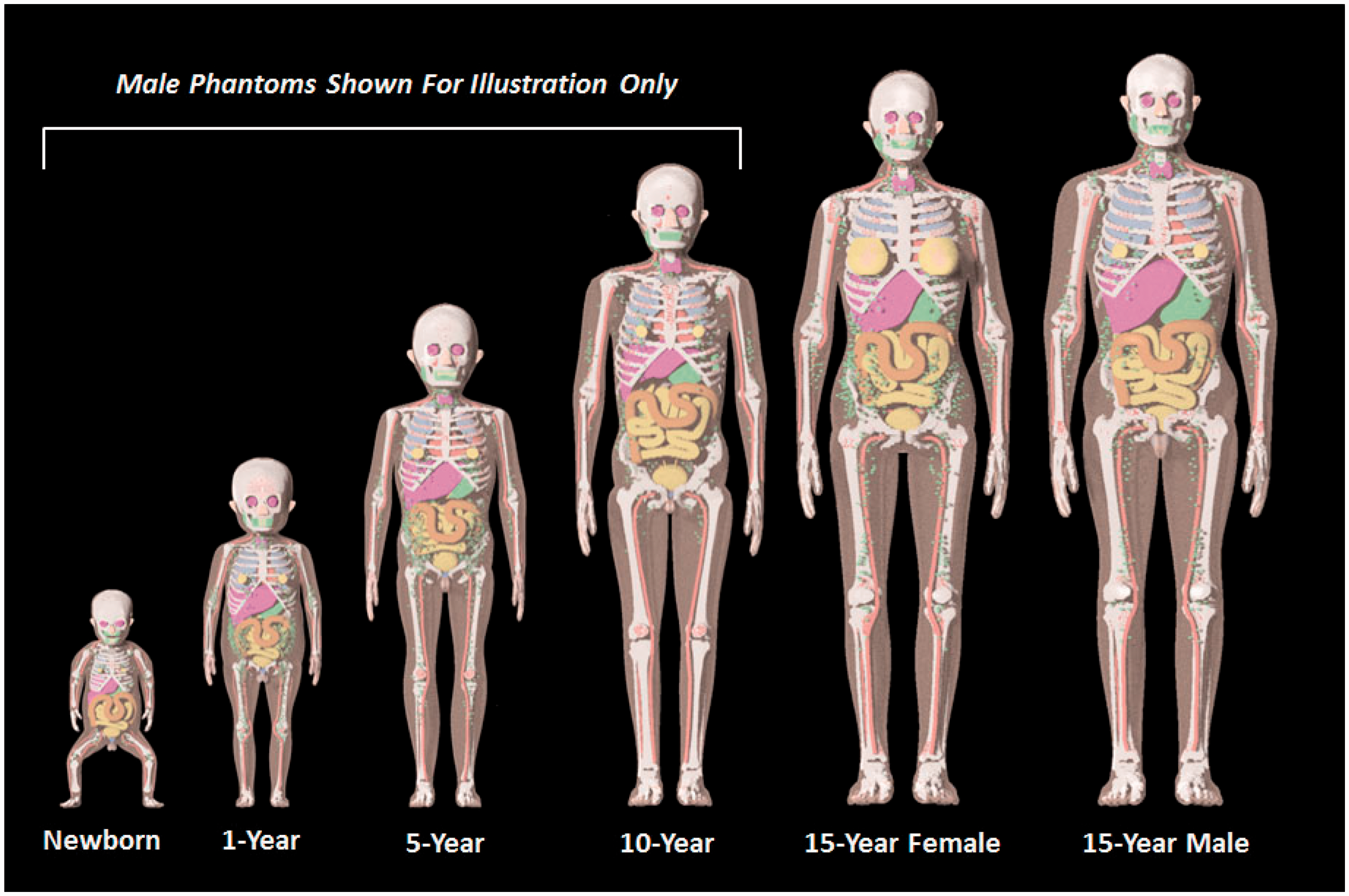
(22) Steps 8 and 9 of phantom development included various modifications to the UF/NCI series of paediatric reference phantoms to ensure conformity to the structure and computational format established in Publication 110 (ICRP, 2009) for the ICRP adult reference computational phantoms. As Publication 89 (ICRP, 2002) was used as guidance for paediatric phantom construction, a significant majority of organs within the Publication 110 phantoms were already present within the UF/NCI paediatric phantoms. Notable exceptions included tissue structures of the breast, colon, lungs, skin, ureters, and major blood vessels. (23) In the UF/NCI phantoms, the breast was modelled as a homogeneous tissue region, while in the Publication 110 (ICRP, 2009) adult female phantom, the breast included both an adipose and glandular tissue compartment. Accordingly, the breasts of the 15-year-old male and female phantoms were thus remodelled into their glandular and adipose regions. Publication 89 (ICRP, 2002) does not give reference masses for the breasts at ages below 15 years, and thus small tissue regions were placed in these phantoms as described by Lee et al. (2010). The colon of the UF/NCI paediatric phantoms was modelled as the right colon, left colon, and rectosigmoid colon, whereas in Publication 110, the adult phantoms were presented with the colon as the ascending colon, transverse colon, descending colon, and rectum. The colon in the UF/NCI series was thus changed to mirror these divisions within the adult reference phantoms. In the UF/NCI phantoms, the lung was modelled as a homogenous structure, while in the reference adult phantoms, there are segmented regions of pulmonary blood vessels. These adult structures of pulmonary blood vessels were thus taken from the adult phantoms, proportionally scaled, and then inserted within the lungs of paediatric phantoms. In the UF/NCI phantoms, the skin was treated as a single tagged structure, whereas in the reference adult phantoms, the skin was tagged separately for regions of the head, trunk, arms, and legs. This four-region separation of the skin was thus implemented in the paediatric phantom series. Finally, the ureters were added to paediatric reference phantoms, as they were not present within the UF/NCI phantom series. The development of models for the major blood vessels is described in Wayson (2012). (24) Lymphatic nodes were added to the UF/NCI paediatric phantom series following the algorithm of Lee et al. (2013), which defined 16 cluster locations within each phantom: ET, cervical, thoracic (upper and lower), breast (left and right), mesentery (left and right), axillary (left and right), cubital (left and right), inguinal (left and right), and popliteal (left and right). Reference values of lymphatic node number and node size were derived from information given in Publications 23 and 89 (ICRP, 1975, 2002). Lymphatic nodes generated by the algorithm of Lee et al. (2013) were applied post-voxelisation via a voxel tagging approach. (25) In the original design of the UF/NCI paediatric phantoms, a residual soft tissue region was defined as a homogeneous mixture between adipose tissue and skeletal muscle in a manner similar to that of the Oak Ridge National Laboratory stylised phantoms. With the adoption of the UF/NCI phantoms by the Commission, a separation of skeletal muscle and subcutaneous/intra-abdominal fat was required. For this purpose, a voxel growing algorithm was introduced to appropriate bones of the skeleton. The final models were reviewed for anatomic accuracy in comparison with equivalent cross-sectional images of the Publication 110 (ICRP, 2009) phantoms in which skeletal muscle was segmented directly from the original CT image sets. The procedure for the revised skeletal muscle model is described in Stepusin (2016). (26) Visual representations of the reference paediatric phantoms are shown in Figs 3.2 and 3.3 below. Fig. 3.2 shows frontal images of the UF/NCI paediatric reference phantoms in their original NURBS/PM format prior to Step 7 voxelisation. For phantoms below the age of 15 years, only the male phantoms are shown. The female phantoms at this age have identical body size and internal anatomy, with the obvious exception of the sex organs. Fig. 3.3 shows frontal views of the final ICRP paediatric reference phantoms in their voxelised format. Again, for ages below 15 years, only the male phantoms are shown, while there are 10 paediatric reference phantoms in total. University of Florida/US National Cancer Institute series of reference paediatric computational phantoms in their non-uniform rational basis spline and polygon mesh formats (prior to Step 7 voxelisation). International Commission on Radiological Protection series of reference paediatric voxel-based computational phantoms (following Step 7 voxelisation and Steps 8 and 9 modification).
Skeletal tissue model for the reference 10-year-old male and female phantoms.
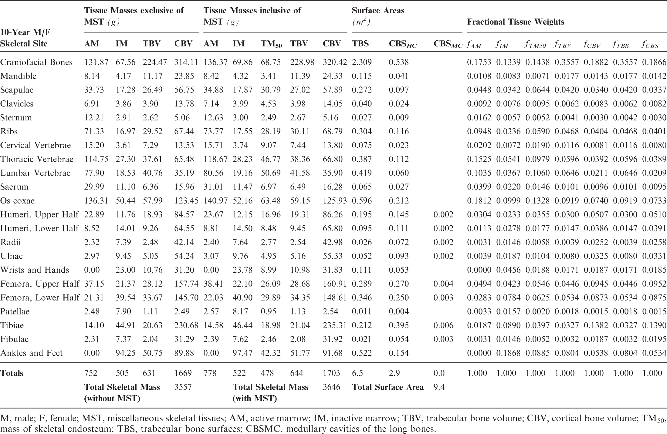
M, male; F, female; MST, miscellaneous skeletal tissues; AM, active marrow; IM, inactive marrow; TBV, trabecular bone volume; CBV, cortical bone volume; TM50, mass of skeletal endosteum; TBS, trabecular bone surfaces; CBSMC, medullary cavities of the long bones.
Skeletal tissue model for the reference 15-year-old male phantom.
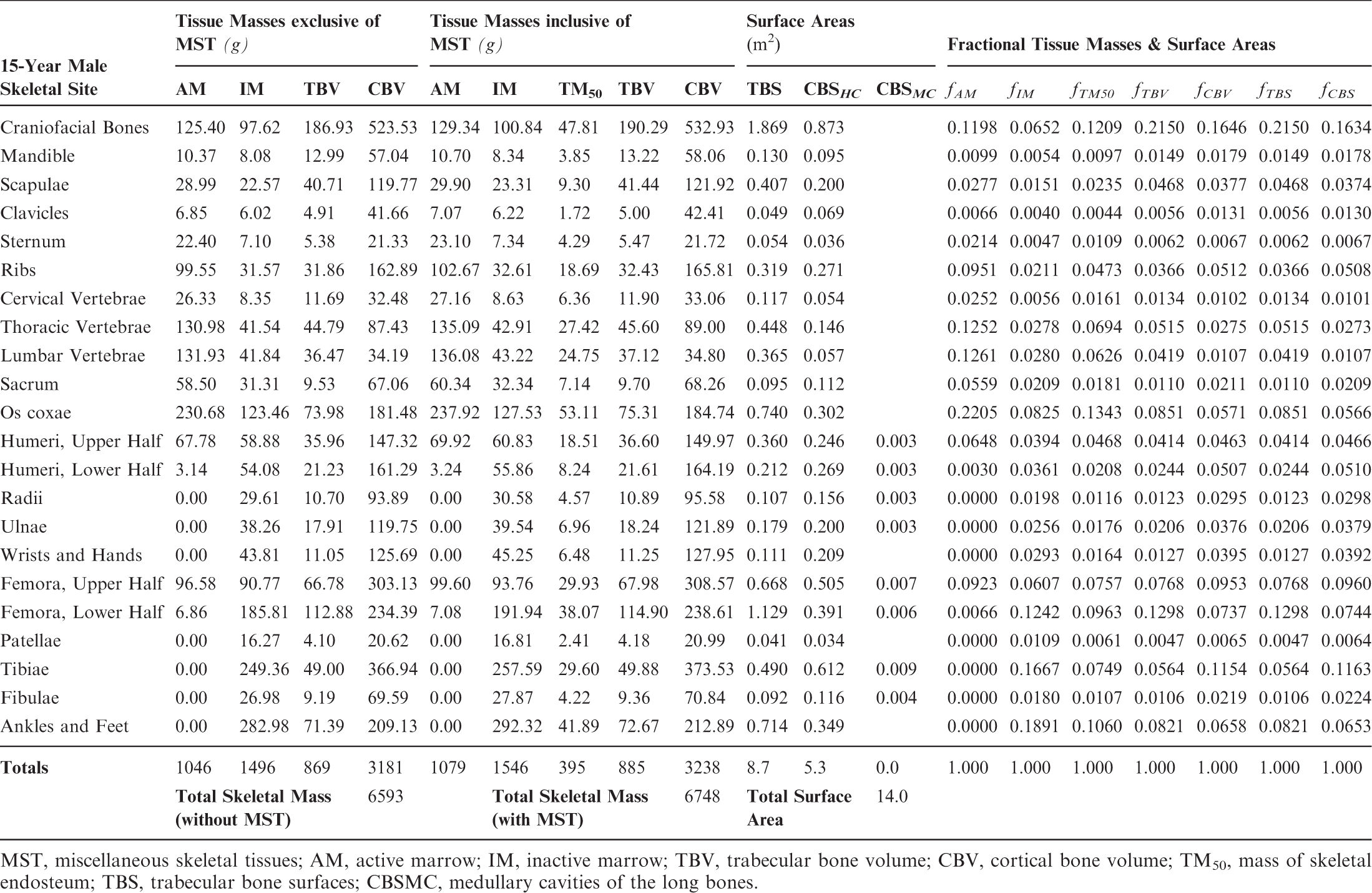
MST, miscellaneous skeletal tissues; AM, active marrow; IM, inactive marrow; TBV, trabecular bone volume; CBV, cortical bone volume; TM50, mass of skeletal endosteum; TBS, trabecular bone surfaces; CBSMC, medullary cavities of the long bones.
Skeletal tissue model for the reference 15-year-old female phantom.
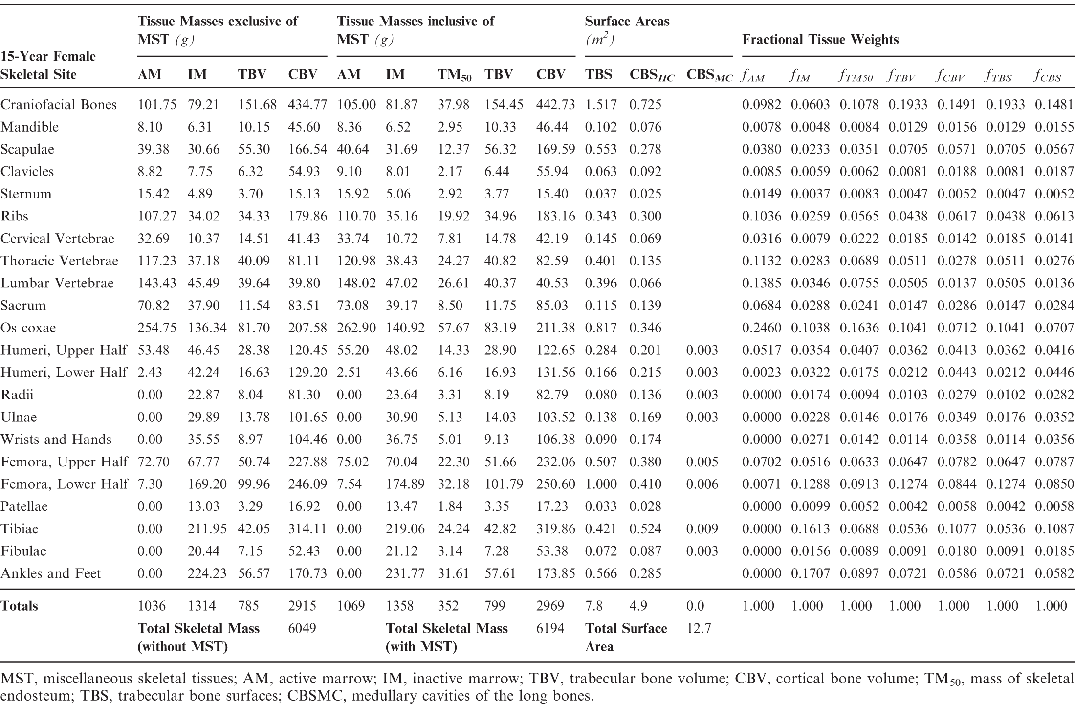
MST, miscellaneous skeletal tissues; AM, active marrow; IM, inactive marrow; TBV, trabecular bone volume; CBV, cortical bone volume; TM50, mass of skeletal endosteum; TBS, trabecular bone surfaces; CBSMC, medullary cavities of the long bones.
4. DESCRIPTION OF THE ICRP PAEDIATRIC REFERENCE PHANTOMS
4.1. Main characteristics of the paediatric phantoms
(27) The orientation of the three-dimensional voxel array (arranged in columns, rows, and slices) describing each member of the paediatric computational phantom series is as follows. The columns correspond to the x coordinates, the rows correspond to the y coordinates, and the slices correspond to the z coordinates. Column numbers increase from right to left, row numbers increase from front to back, and slice numbers increase from the toes to the vertex of the body. This convention is equivalent to that established in Publication 110 (ICRP, 2009) for the reference adult computational phantoms. (28) The main characteristics of the paediatric reference computational phantoms are given in Table 4.1 which summarises the final voxel resolution, voxel count, and total matrix size of each of the reference paediatric phantoms, along with the same parameters for the adult reference phantoms of Publication 110 (ICRP, 2009). A goal of the paediatric phantom series was to limit the total matrix size to approximately 55 million voxels, while maintaining the in-plane voxel size to approximately the reference skin thickness at each phantom age. For the newborn reference phantoms (both male and female), isotropic voxels of 0.663 mm on edge were employed. For the remaining phantoms, the in-plane resolution was again set at the reference total skin thickness, allowing the z dimension of the voxels to vary while maintaining the imposed limit on the total matrix size. The higher resolution of the paediatric phantoms, due to their method of construction, is evident in comparison with the total matrix sizes of the Publication 110 adult phantoms: 7.16 and 14.26 million voxels for the adult male and adult female, respectively. (29) Table 4.2 shows a list of the source and target regions of the series of 10 paediatric reference phantoms, their segmented volumes, and resulting tissue masses. For comparison, ICRP reference masses are also shown. Main characteristics of the reference paediatric computational phantoms. M, male; F, female; P110, ICRP Publication 110. The newborn phantoms have legs that are bent, and thus the “height” is more appropriately the phantom “length”.
4.2. Skeletal source regions
(30) For internal sources in the skeleton, the following source regions have to be considered: cortical bone (surface or volume), trabecular bone (surface or volume), and cortical and trabecular bone marrow. As discussed in Publication 110 (ICRP, 2009), no distinction is made between surface and volume sources in the cortical and trabecular regions of the computational phantoms. The results from the respective volume sources are to be applied to estimate values for the bone surface sources when using the computational reference phantoms for radiation transport simulations. A cortical bone volume has been defined separately in all bones and bone groups of the skeleton, and thus the entirety of these voxels can be used directly to sample a uniform source distribution. (31) As described previously, trabecular bone is one of the constituents that make up the spongiosa. Therefore, the entirety of the spongiosa voxels of all bones serves as the volume which can be sampled for particle emission. However, as the relative amount of trabecular bone in the spongiosa varies between individual bones and bone groups, and across the age-dependent phantom series, the source should not simply be assumed to be distributed homogeneously. For Monte Carlo radiation transport calculations, the variation of trabecular bone mass fraction should be used (e.g. either to determine the probability of a start position being selected, or to assign bone-specific initial statistical weights to the particles starting in the spongiosa volumes of the various regions of the skeleton). Fractional tissue masses and bone surface areas provided in Tables 3.3–3.8 may be used for this purpose. (32) For cortical marrow, medullary cavities have been defined in the shafts of the long bones, so the entirety of these segmented voxels can be used directly to sample a uniform source distribution. While the medullary cavities contain only inactive (yellow) marrow in the adult models of Publication 110 (ICRP, 2009), the marrow cellularities vary with reference age and long bone site as given in Publication 70 (ICRP, 1995). (33) Trabecular marrow is the marrow situated in the spongiosa regions of the skeleton. Consequently, the same particle source sampling principle as for trabecular bone should be applied for trabecular marrow, now considering the bone-specific relative bone marrow content (active and inactive marrow). The fractional tissue masses of Tables 3.3–3.8 may be used for this purpose.
List of source and target regions, their segmented volumes, and resulting masses compared with the reference masses of Publication 89.
M, male; F, female.
Some of the reference values (e.g. blood and lymphatic tissue) duplicate other mass information and are, thus, not additive.
Segmented blood vessels vs total blood (partly included in the organ).
Segmented lymph nodes vs ‘fixed' lymphatic tissue including lymphatic ducts and lymph.
Segmented directly.
Incorporated in spongiosa regions.
Partly segmented directly and partly incorporated in spongiosa regions.
4.3. Skeletal target regions
(34) The skeletal target tissues of interest are the active (red) bone marrow and the endosteal tissues (formerly called ‘bone surfaces’). As the dimensions of the marrow cavities and the endosteal layer lining these cavities (assumed to be of thickness 50 µm) are clearly finer than the resolution of the voxelised computational phantoms, they cannot be represented directly and have to be considered in the homogeneous tissues of the spongiosa volumes. However, in contrast to the source volumes described above, it is not sufficient to consider the bone-specific relative amounts of these tissues in the spongiosa. The reason is that secondary particle disequilibria may exist for photon and neutron irradiation of the skeleton. For photons, these typically take the form of dose enhancement with photoelectron interactions favouring interaction sites in bone trabeculae. For neutrons, these typically take the form of dose suppression with the hydrogen elastic scattering favouring interaction sites in the marrow tissues. Specific techniques for assessing photon and neutron dose in the skeletal tissues of the reference adults are reviewed in Annexes E and F of Publication 116 (ICRP, 2010), respectively. Techniques for application to the reference paediatric phantoms have been developed and will be reported in a forthcoming ICRP publication.
Reference values for regional blood distribution (% total blood volume) for the ICRP reference persons
4.4. Model of regional blood distribution
(35) As was the case for the adult reference phantoms of Publication 110 (ICRP, 2009), it is not possible to fully represent the entire blood pool of the body within the voxelised structures of the paediatric reference computational phantoms. As described in Wayson (2012), an attempt was made to place NURBS tubular structures within the paediatric phantom series to represent the major blood vessels of the body. No attempt was made to segment the blood vessels in the original CT images during initial phantom construction due to image resolution limitations. A significant portion of the total body blood volume is thus situated in the smaller vessels and capillaries within most organs and tissues, and these vascular structures are not modelled explicitly in the paediatric reference phantom series. As noted in Publication 110, organ elemental compositions given in Publication 89 (ICRP, 2002) and in ICRU Report 46 (ICRU, 1992) are exclusive of organ blood content, and thus are relevant to organ parenchyma alone. (36) This publication has followed the methodology of Section 5.3 in Publication 110 (ICRP, 2009) in which the elemental compositions of the organs and tissues of the reference computational phantoms have been computed as a homogeneous mixture of the elemental compositions of the organ parenchyma and their intra-organ blood content. To accomplish this step, values of the fractional distribution of total blood amongst the organs and tissues of the body need to be assigned. Publication 89 (ICRP, 2002), however, provides this data for reference adults alone. In work described in Wayson (2012), age-dependent values for regional blood distribution have been derived, as shown in Table 4.3. These values were derived via organ volume proportional scaling of the adult values (male and female computed separately), with additional consideration of age-dependent vascular growth in the brain, kidneys, and skeletal tissues. Final values of the phantom-specific and tissue-specific elemental compositions are given in Annex B of this publication.
4.5. Phantom limitations
(37) As with the adult reference computational phantoms of Publication 110 (ICRP, 2009), there are also limitations of the paediatric phantom series of this publication due to their voxelised nature. As described in Section 5.4 of Publication 110, the majority of the limitations in the adult reference phantoms were attributed to the corresponding limitations in CT image resolution from which the phantoms were constructed. As outlined in Fig. 3.1 of this publication, however, the revised process of NURBS/PM surface modelling and subsequent voxelisation of the paediatric reference phantoms allowed for significant improvements in matching phantom organ mass to their reference values over that seen in the adult phantoms. Notable exceptions, as outlined in Lee et al. (2010), included an underestimate of the reference content masses of the gastrointestinal tract organs: stomach contents in the newborn phantoms; small intestine contents in the newborn, 1-year-old, and 5-year-old phantoms; and colon contents in the full series of paediatric phantoms. However, reference values of gastrointestinal tract organ wall masses and lengths were preserved to within a few percent of reference values. Other limitations are noted in an underestimate of the heart contents of the newborn phantoms, and the urinary bladder contents in the newborn and 1-year-old phantoms. Skin masses are also not in compliance with their reference values, in which reference total skin masses of the newborn and 1-year-old phantoms are underestimated, while they are overestimated in the 5-year-old, 10-year-old, and 15-year-old phantoms. As described in Lee et al. (2010), the original design of the phantoms did not permit simultaneous matching of both reference skin mass and reference skin thickness. The latter was deemed more appropriate, particularly for applications of external dosimetry, and was thus given preference in the phantom design. Finally, as with the adult reference phantoms, the microscopic target regions of the skeleton, respiratory tract, and alimentary tract organs (including their stem cell targets) are not modelled in the voxelised structures of the paediatric reference phantom series. As such, supplemental models of these tissue regions as given in Pafundi (2009), Publication 66 (ICRP, 1994), and Publication 100 (ICRP, 2006) continue to be applied for computation of SAF values for internal exposures.
5. APPLICATIONS AND LIMITATIONS OF THE PAEDIATRIC REFERENCE PHANTOMS
(38) The phantoms presented in this publication are the official computational models representing the 10-member paediatric series of reference individuals – male and female newborn, 1-year-old, 5-year-old, 10-year-old, and 15-year-old. These reference computational models are based on CT data of real individuals and hence represent digital three-dimensional representations of human anatomy. They are defined to enable calculations of the protection quantities – organ and tissue equivalent dose, and effective dose – from exposure to ionising radiations. The Commission will publish recommended values of dose coefficients for both external and internal environmental exposures using this series of paediatric reference phantoms. These publications will include SAFs for particles relevant to internal exposures, and dose coefficients for externally incident environmental radiation fields. (39) It should be clear that although these phantoms have organ masses of reference values, they still have individual organ topology (organ shape, depth, and position) reflecting the CT data used in their construction. Resultantly, these models cannot be used to assess organ doses in individuals of differing body size and organ morphometry. While reference computational phantoms were created for the purpose of deriving radiological protection quantities, it is acknowledged that these phantoms have broader applications. However, one must be mindful of the specific limitations related to their intended application.
REFERENCES
ANNEX A. IDENTIFICATION (ID) NUMBER LISTINGS, MEDIUM, DENSITY, MASS, MINIMUM/MAXIMUM COLUMNS, ROWS, AND SLICES OCCUPIED BY EACH ORGAN/TISSUE (CONTAINING RECTANGULAR PRISM), AND ORGAN CENTRES OF MASS
(A1) Table A.1 lists the organ ID number, medium, and mass of each organ/tissue. The organ ID is the number stored in the voxel array at the positions of those voxels belonging to the respective organ/tissue. For the purpose of radiation transport calculations, a material composition has to be assigned to the organs/tissues. The ‘medium’ numbers given here refer to the elemental compositions of Annex B. (A2) Furthermore, for each organ, a rectangular prism (box) containing the organ (minimum/maximum columns, rows, and slices occupied by the organ/tissue) is given to facilitate the sampling of internal sources. Finally, the organ’s centre of mass (in terms of both voxels and coordinate position) is also given (Tables A.2–A.11 for all paediatric reference phantoms). (A3) The orientation of the three-dimensional voxel array describing the computational phantom is as follows. The columns correspond to the x coordinates, the rows correspond to the y coordinates, and the slices correspond to the z coordinates. Column numbers increase from right to left, row numbers increase from front to back, and slice numbers increase from the toes to the vertex of the body. Identification (ID) number listings, medium, and mass of each organ/tissue. ET, extrathoracic. Identification (ID) number listings, rectangular prism (box) containing the organ (minimum/maximum columns, rows, and slices occupied by each organ/tissue), and organ centres of mass (in terms of voxels as well as coordinates) for the newborn male phantom. ET, extrathoracic. Identification (ID) number listings, rectangular prism (box) containing the organ (minimum/maximum columns, rows, and slices occupied by each organ/tissue), and organ centres of mass (in terms of voxels as well as coordinates) for the newborn female phantom. ET, extrathoracic. Identification (ID) number listings, rectangular prism (box) containing the organ (minimum/maximum columns, rows, and slices occupied by each organ/tissue), and organ centres of mass (in terms of voxels as well as coordinates) for the 1-year-old male phantom. ET, extrathoracic. Identification (ID) number listings, rectangular prism (box) containing the organ (minimum/maximum columns, rows, and slices occupied by each organ/tissue), and organ centres of mass (in terms of voxels as well as coordinates) for the 1-year-old female phantom. ET, extrathoracic. Identification (ID) number listings, rectangular prism (box) containing the organ (minimum/maximum columns, rows, and slices occupied by each organ/tissue), and organ centres of mass (in terms of voxels as well as coordinates) for the 5-year-old male phantom. ET, extrathoracic. Identification (ID) number listings, rectangular prism (box) containing the organ (minimum/maximum columns, rows, and slices occupied by each organ/tissue), and organ centres of mass (in terms of voxels as well as coordinates) for the 5-year-old female phantom. ET, extrathoracic. Identification (ID) number listings, rectangular prism (box) containing the organ (minimum/maximum columns, rows, and slices occupied by each organ/tissue), and organ centres of mass (in terms of voxels as well as coordinates) for the 10-year-old male phantom. ET, extrathoracic. Identification (ID) number listings, rectangular prism (box) containing the organ (minimum/maximum columns, rows, and slices occupied by each organ/tissue), and organ centres of mass (in terms of voxels as well as coordinates) for the 10-year-old female phantom. ET, extrathoracic. Identification (ID) number listings, rectangular prism (box) containing the organ (minimum/maximum columns, rows, and slices occupied by each organ/tissue), and organ centres of mass (in terms of voxels as well as coordinates) for the 15-year-old male phantom. ET, extrathoracic. Identification (ID) number listings, rectangular prism (box) containing the organ (minimum/maximum columns, rows, and slices occupied by each organ/tissue), and organ centres of mass (in terms of voxels as well as coordinates) for the 15-year-old female phantom. ET, extrathoracic.
ANNEX B. LIST OF MEDIA AND THEIR ELEMENTAL COMPOSITIONS
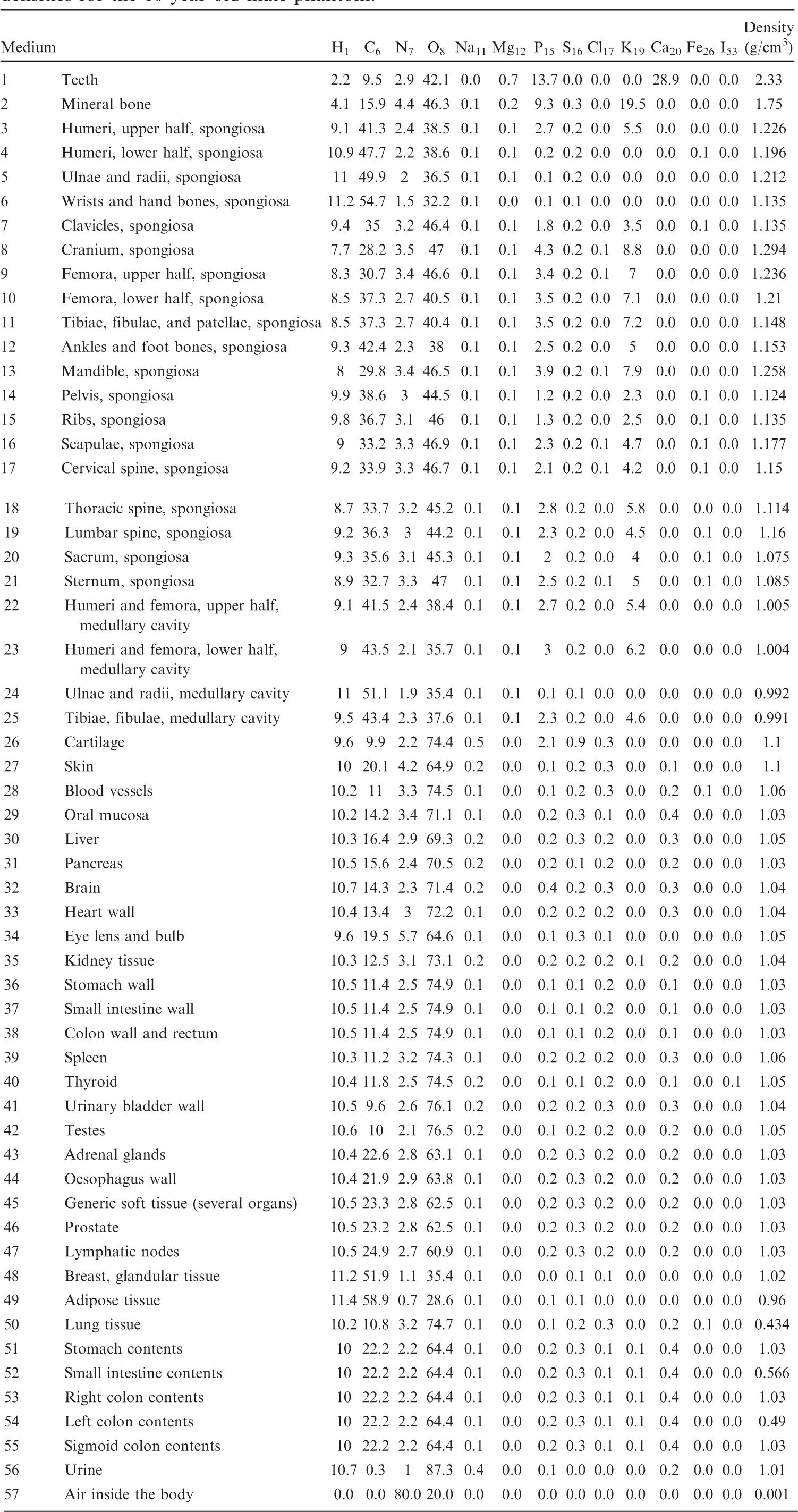
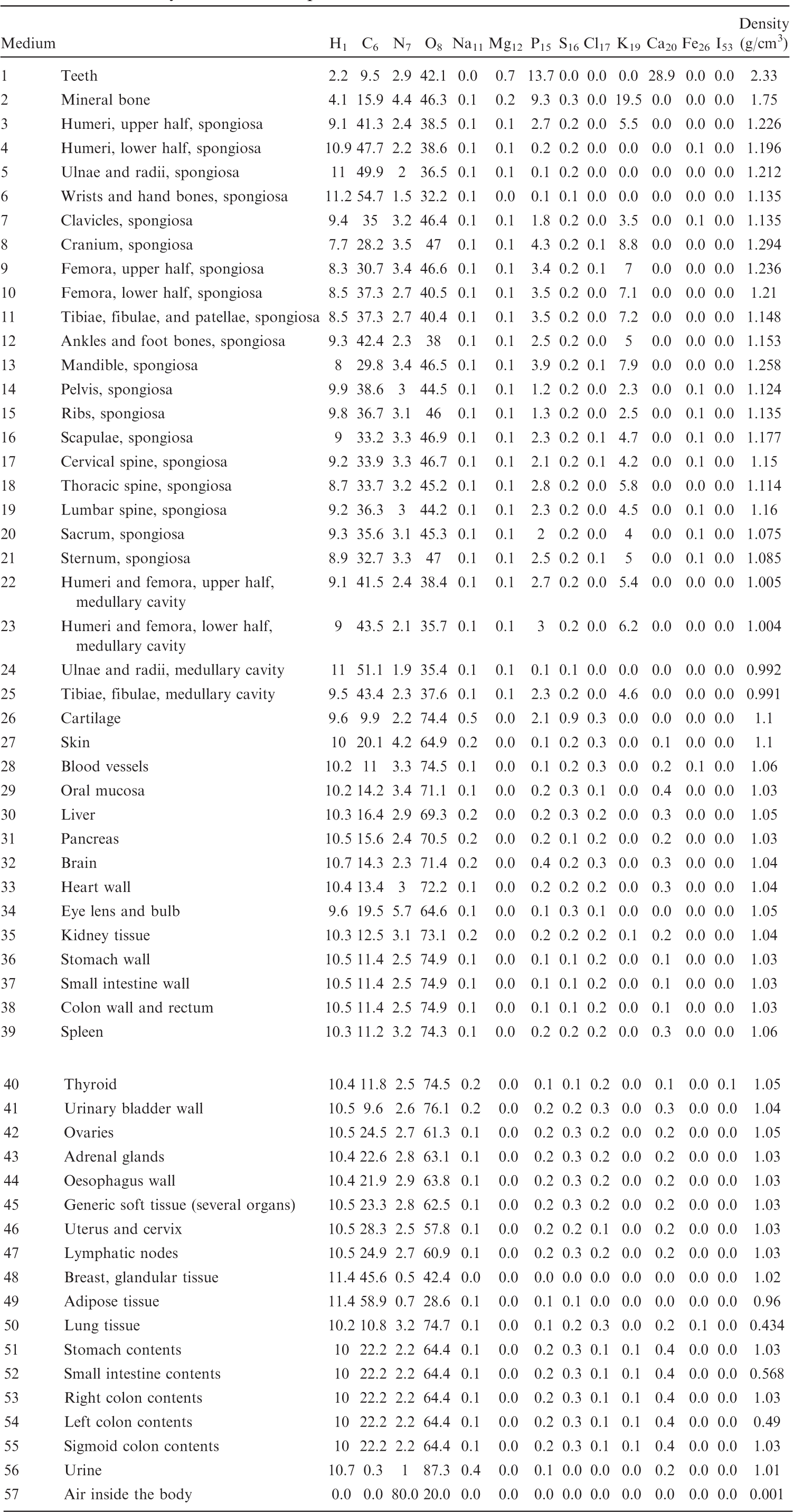
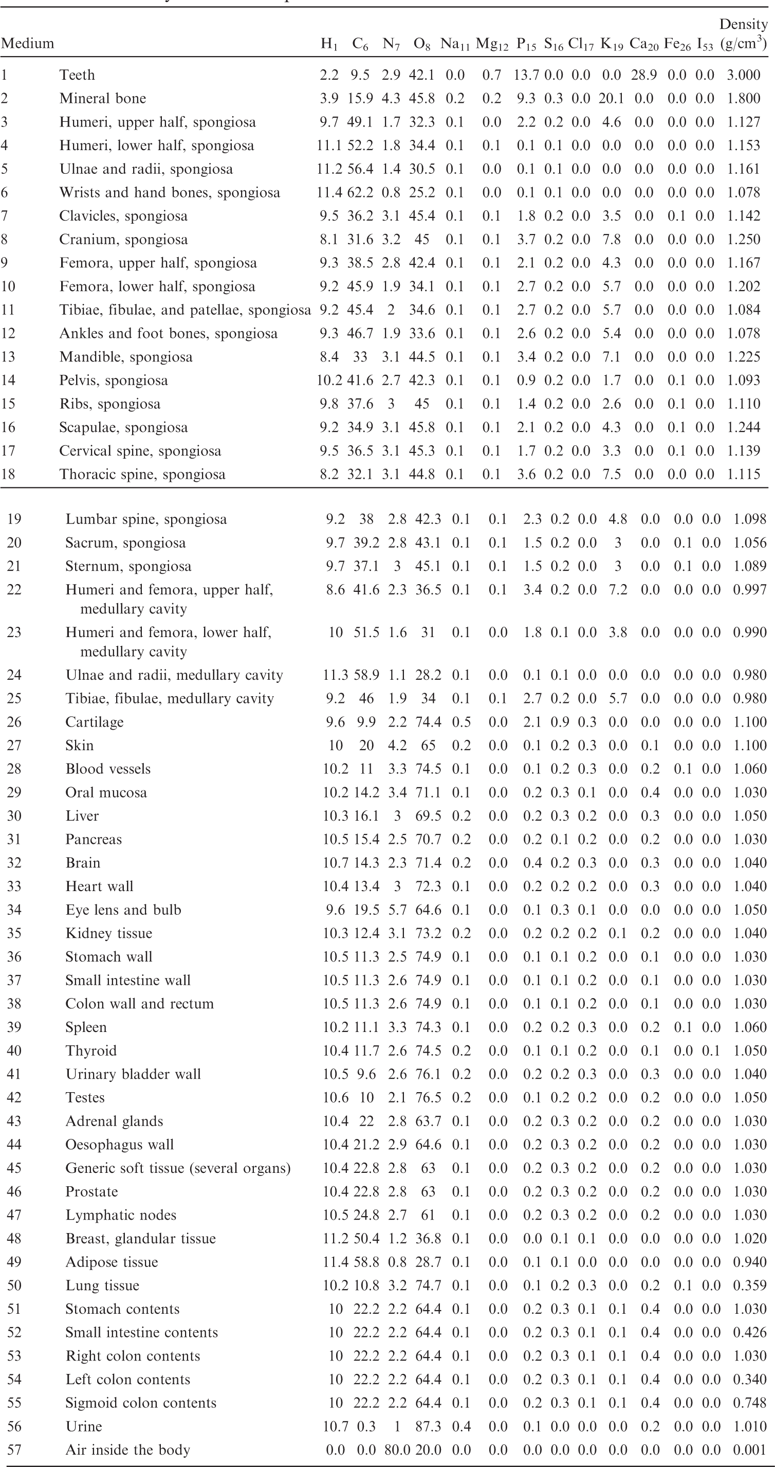
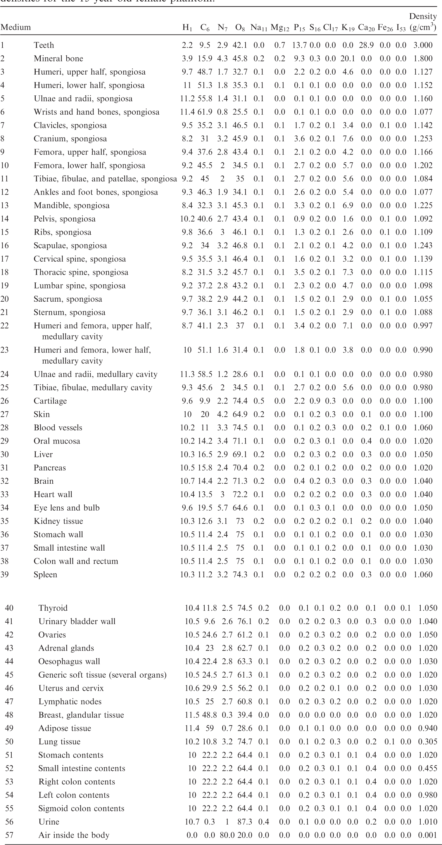
(B1) For the purpose of radiation transport calculations, each organ/tissue must have a certain elemental material composition. Therefore, a list of media has been defined that are assigned to the various organ IDs as assigned in Table A.1. Tables B.1–B.10 give the elemental composition of the tissue media for the ICRP series of reference paediatric phantoms.
List of media, their elemental compositions (percent by mass), and their mass densities for the newborn male phantom.
List of media, their elemental compositions (percent by mass), and their mass densities for the newborn female phantom.
List of media, their elemental compositions (percent by mass), and their mass densities for the 1-year-old male phantom.
List of media, their elemental compositions (percent by mass), and their mass densities for the 1-year-old female phantom.
List of media, their elemental compositions (percent by mass), and their mass densities for the 5-year-old male phantom.
List of media, their elemental compositions (percent by mass), and their mass densities for the 5-year-old female phantom.
List of media, their elemental compositions (percent by mass), and their mass densities for the 10-year-old male phantom.
List of media, their elemental compositions (percent by mass), and their mass densities for the 10-year-old female phantom.
List of media, their elemental compositions (percent by mass), and their mass densities for the 15-year-old male phantom.
List of media, their elemental compositions (percent by mass), and their mass densities for the 15-year-old female phantom.
ANNEX C. LIST OF SOURCE REGIONS, ACRONYMS, AND IDENTIFICATION NUMBERS
(C1) Table C.1 establishes a set of acronyms for the source regions for the calculation of SAFs. The regions of the Human Alimentary Tract Model and the Human Respiratory Tract Model are listed first, followed by the systemic regions. The third column gives the ID numbers in the phantoms that make up the respective region or – if these are too many – a footnote to this table where the subdivision of the region is expanded in detail.
Source regions, acronyms, and corresponding identification (ID) numbers in the paediatric phantoms.
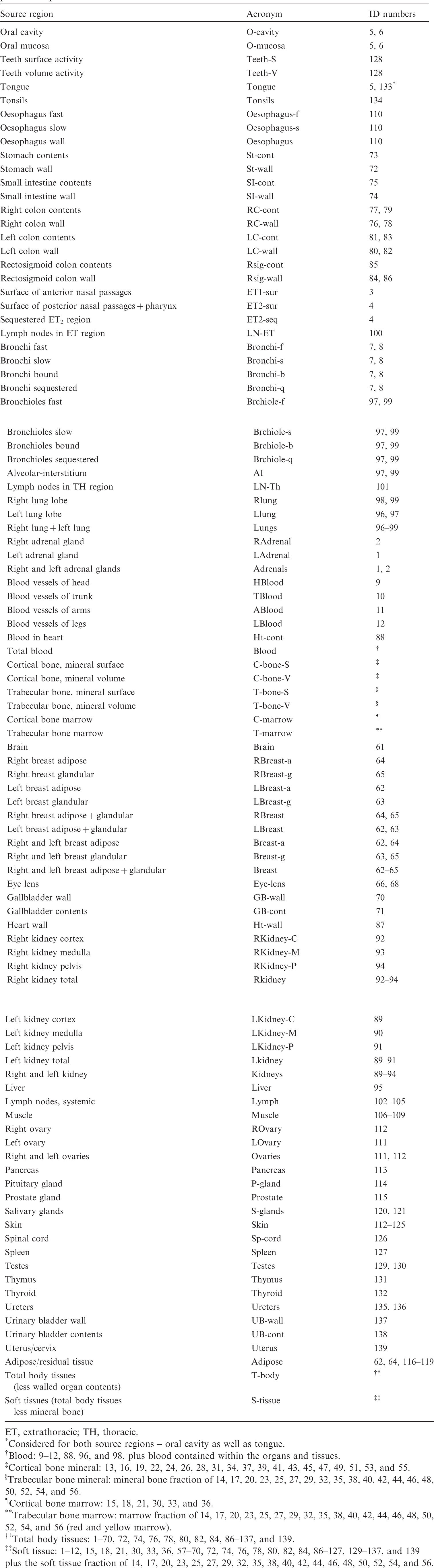
ET, extrathoracic; TH, thoracic.
Considered for both source regions – oral cavity as well as tongue.
Blood: 9–12, 88, 96, and 98, plus blood contained within the organs and tissues.
Cortical bone mineral: 13, 16, 19, 22, 24, 26, 28, 31, 34, 37, 39, 41, 43, 45, 47, 49, 51, 53, and 55.
Trabecular bone mineral: mineral bone fraction of 14, 17, 20, 23, 25, 27, 29, 32, 35, 38, 40, 42, 44, 46, 48, 50, 52, 54, and 56.
Cortical bone marrow: 15, 18, 21, 30, 33, and 36.
Trabecular bone marrow: marrow fraction of 14, 17, 20, 23, 25, 27, 29, 32, 35, 38, 40, 42, 44, 46, 48, 50, 52, 54, and 56 (red and yellow marrow).
Total body tissues: 1–70, 72, 74, 76, 78, 80, 82, 84, 86–137, and 139.
Soft tissue: 1–12, 15, 18, 21, 30, 33, 36, 57–70, 72, 74, 76, 78, 80, 82, 84, 86–127, 129–137, and 139
plus the soft tissue fraction of 14, 17, 20, 23, 25, 27, 29, 32, 35, 38, 40, 42, 44, 46, 48, 50, 52, 54, and 56.
ANNEX D. LIST OF TARGET REGIONS, ACRONYMS, AND IDENTIFICATION NUMBERS
(D1) Table D.1 establishes a set of acronyms for the target regions. The organs contributing to effective dose are listed first, followed by the regions of the Human Alimentary Tract Model, the Human Respiratory Tract Model, and the systemic regions. The third column gives the ID numbers in the phantoms that make up the respective tissue or – if these are too many – a footnote to this table where the subdivision of the tissue is expanded in detail.
Target regions, acronyms, and corresponding identification (ID) numbers in the paediatric phantoms.
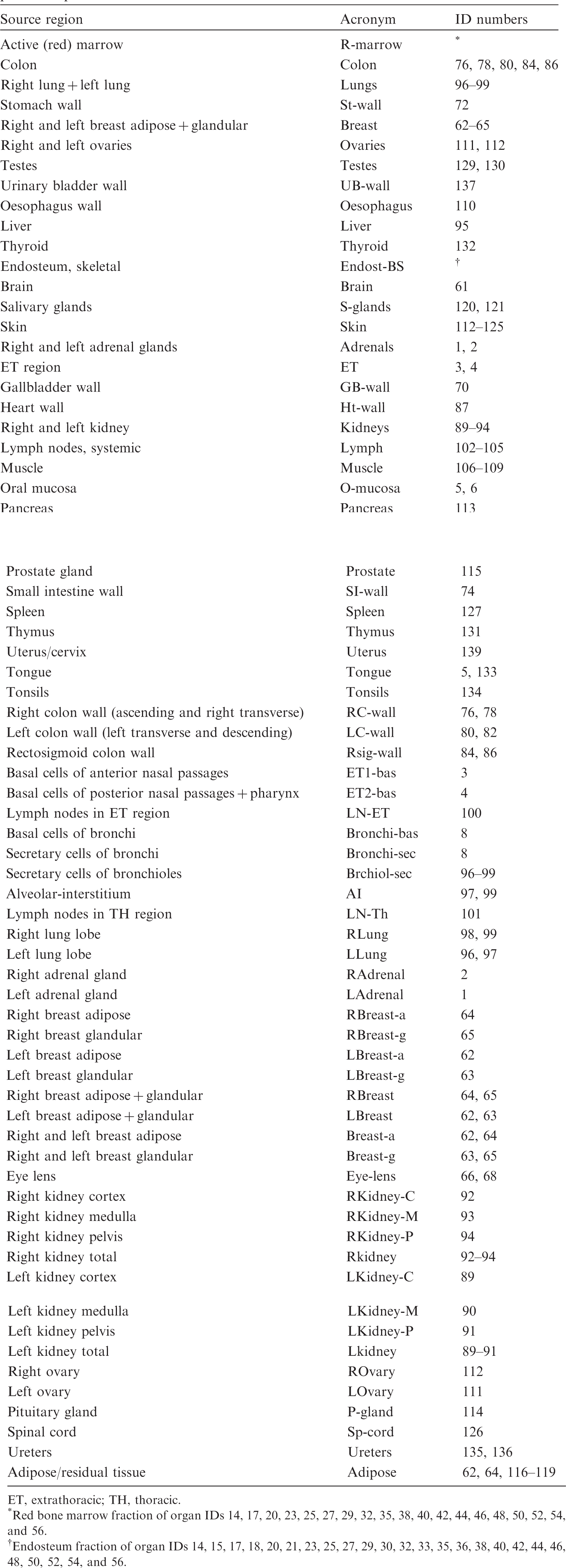
ET, extrathoracic; TH, thoracic.
Red bone marrow fraction of organ IDs 14, 17, 20, 23, 25, 27, 29, 32, 35, 38, 40, 42, 44, 46, 48, 50, 52, 54, and 56.
Endosteum fraction of organ IDs 14, 15, 17, 18, 20, 21, 23, 25, 27, 29, 30, 32, 33, 35, 36, 38, 40, 42, 44, 46, 48, 50, 52, 54, and 56.
ANNEX E. DISTRIBUTIONS OF DEPTHS OF SELECTED ORGANS/TISSUES
(E1) In Figs E.1–E.65, depth distributions below the body surfaces at the front, back, right, left, bottom, and top of the reference paediatric phantoms are shown for those organs and tissues that contribute to effective dose with specific tissue weighting factors, except the endosteal tissues for which no geometrical representation is available in the reference computational phantoms. (E2) The distributions have been evaluated for 10 million points sampled randomly in the organs considered. Due to the curved surface of the body, these depths are not below planar surfaces but below uneven surfaces. They indicate the amount of overlying tissue by which each point of an organ or tissue is shielded from radiation impinging from the front, back, left, right, top, or bottom. (E3) Together with the attenuation properties of the overlying tissues and the organ considered, the depth below the surface is a parameter that significantly influences the dose coefficients from external radiation.
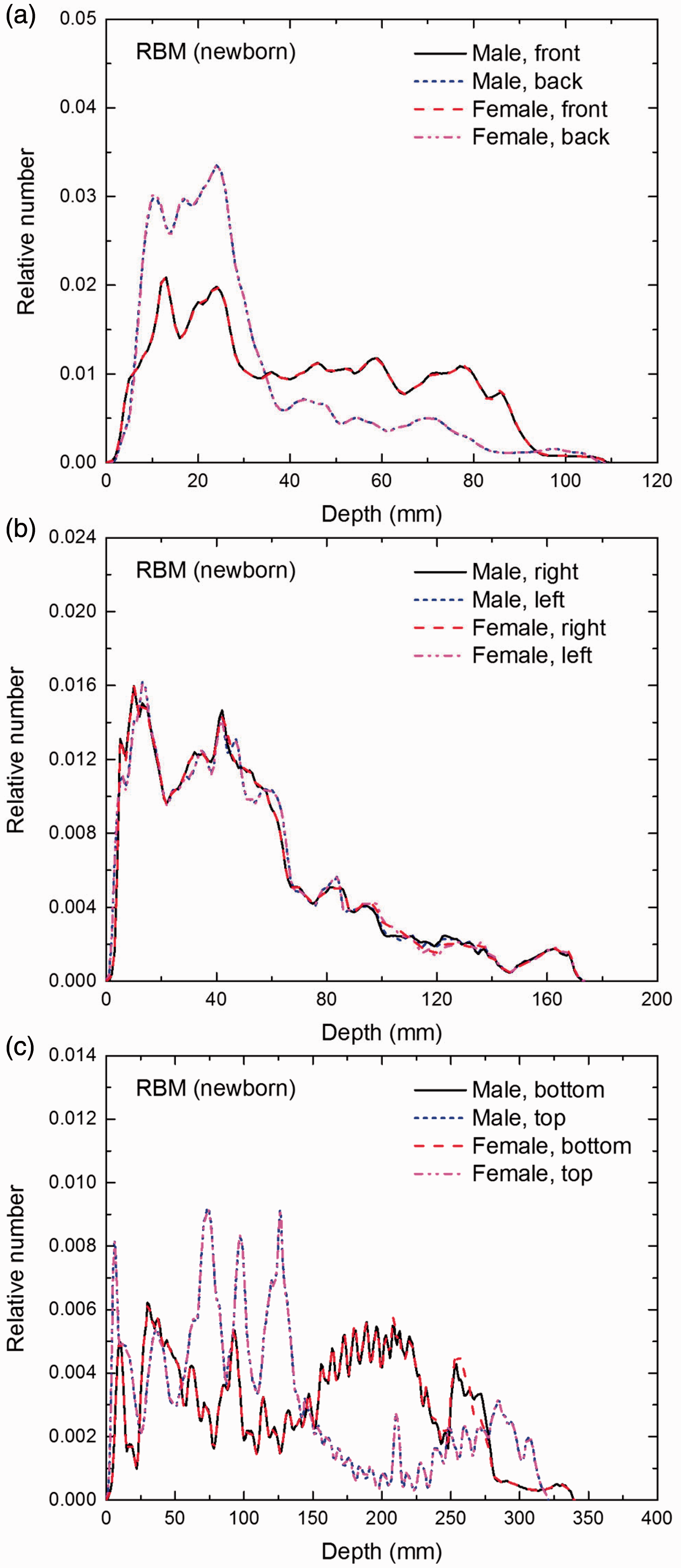
Distribution of depths of 10 million randomly sampled points in the red bone marrow (RBM) below the body surface of the newborn male/female phantoms at: (a) front and back, (b) right and left, and (c) bottom and top.
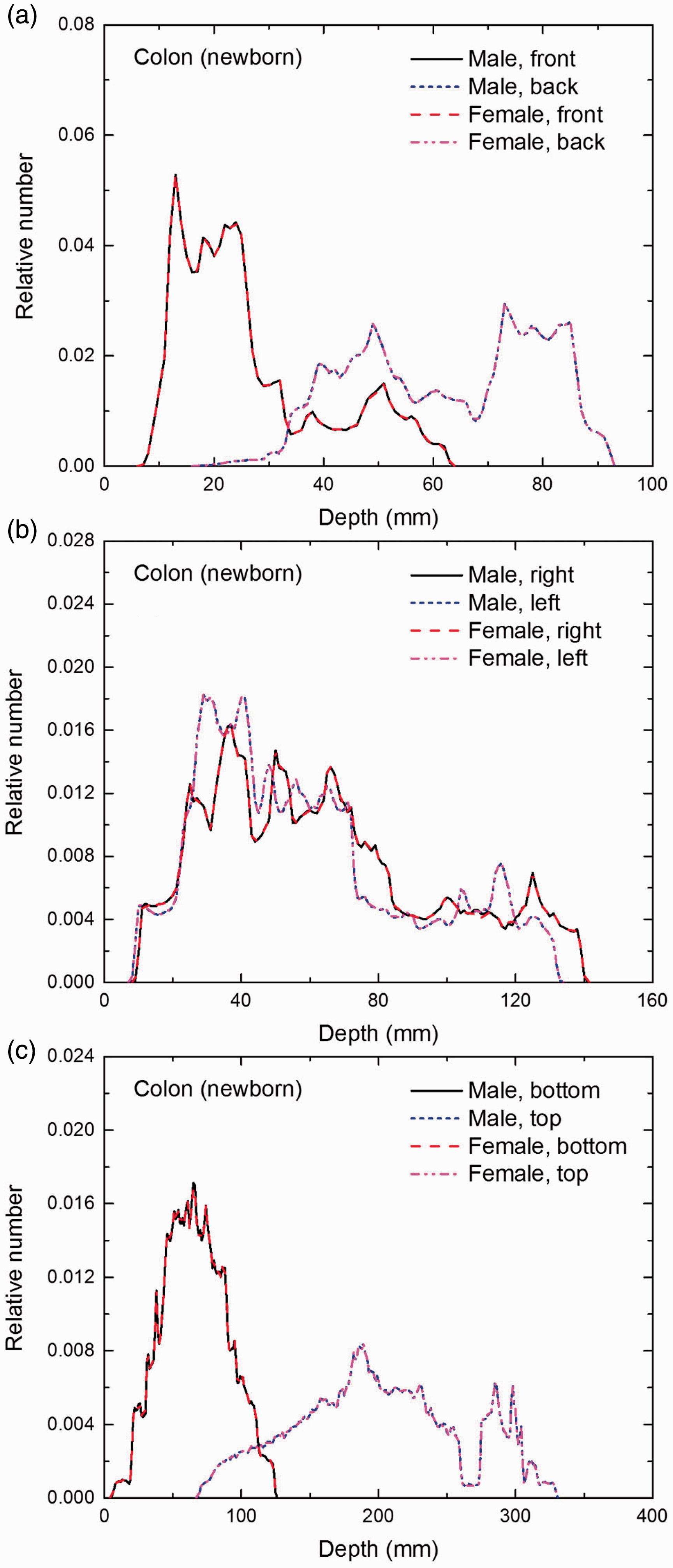
Distribution of depths of 10 million randomly sampled points in the colon wall below the body surface of the newborn male/female phantoms at: (a) front and back, (b) right and left, and (c) bottom and top.
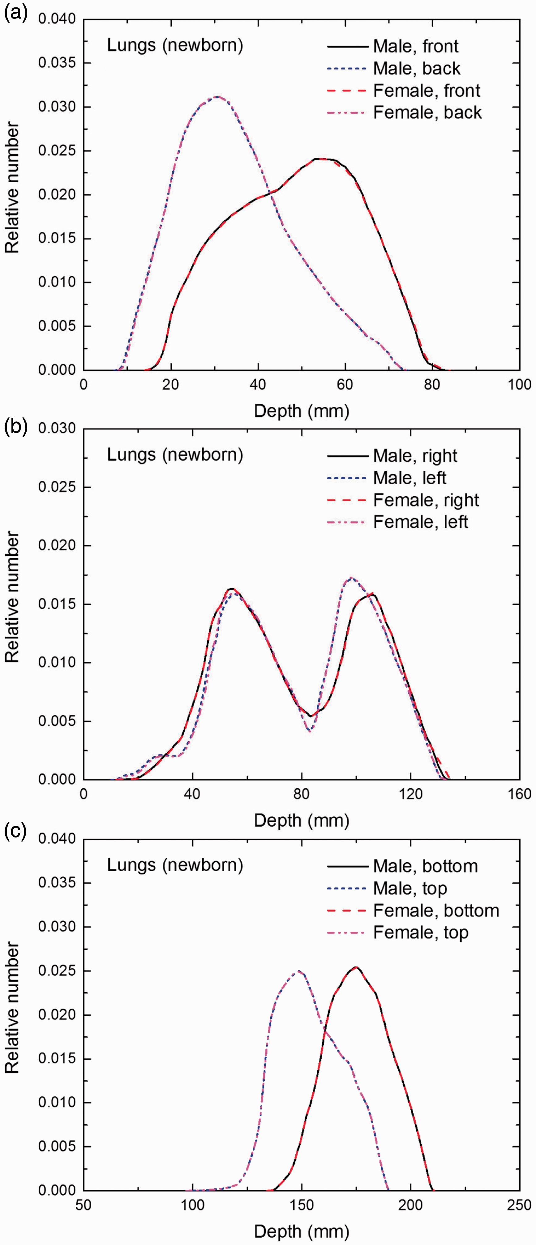
Distribution of depths of 10 million randomly sampled points in the lungs below the body surface of the newborn male/female phantoms at: (a) front and back, (b) right and left, and (c) bottom and top.
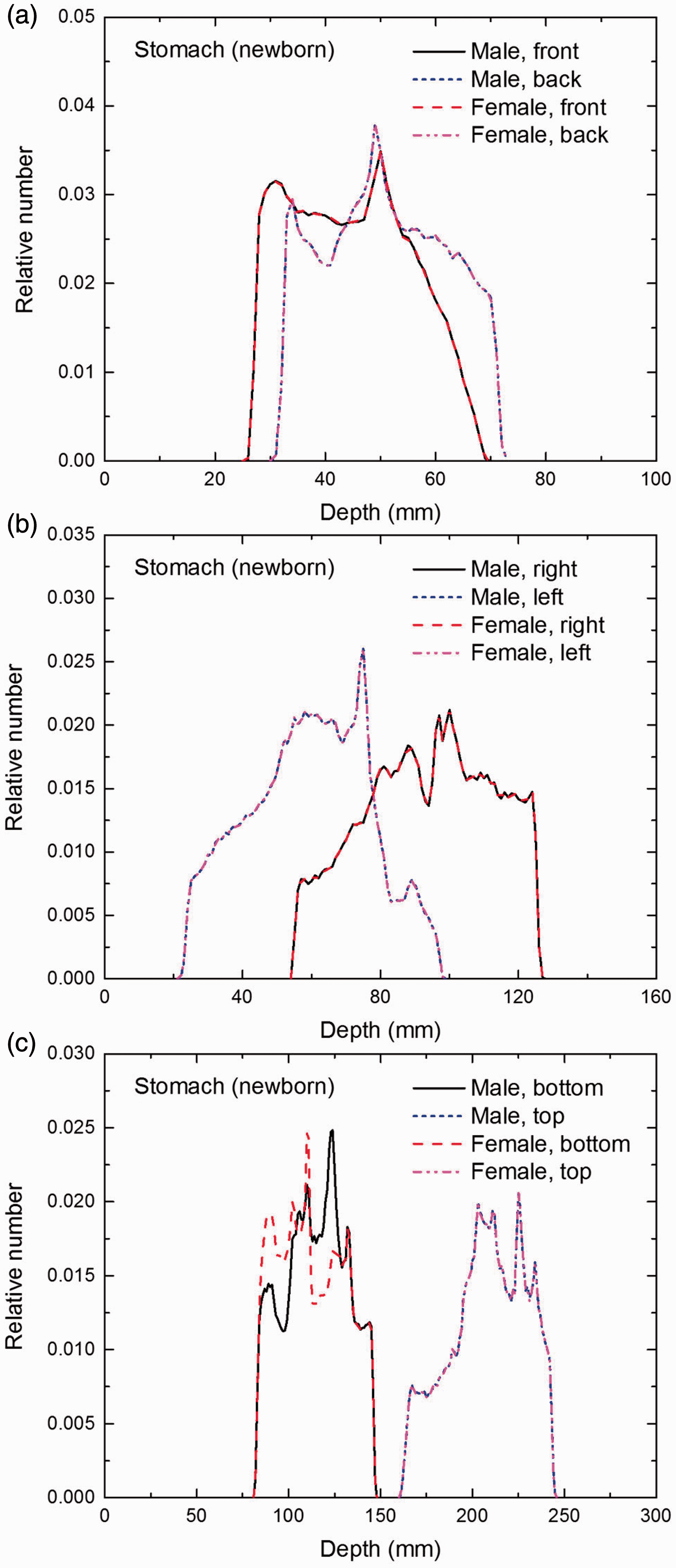
Distribution of depths of 10 million randomly sampled points in the stomach wall below the body surface of the newborn male/female phantoms at: (a) front and back, (b) right and left, and (c) bottom and top.
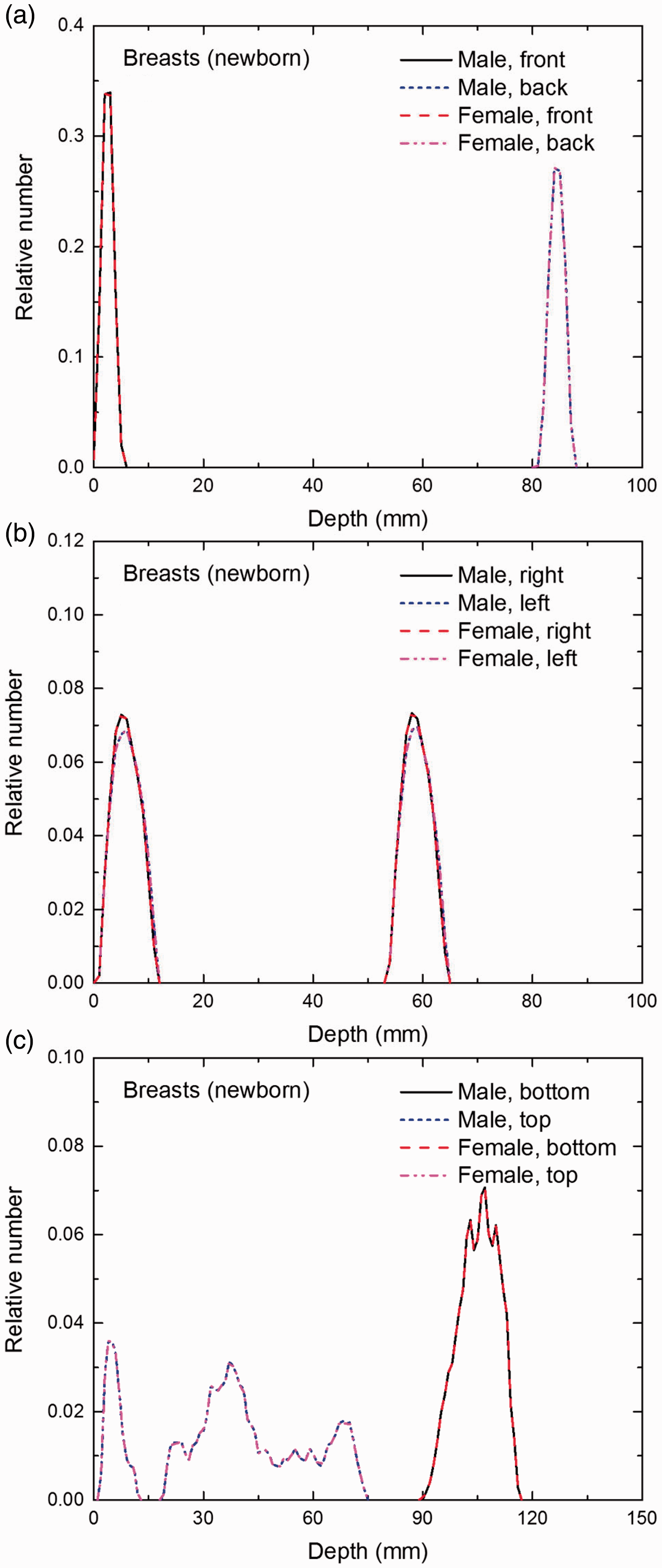
Distribution of depths of 10 million randomly sampled points in the breasts below the body surface of the newborn male/female phantoms at: (a) front and back, (b) right and left, and (c) bottom and top.
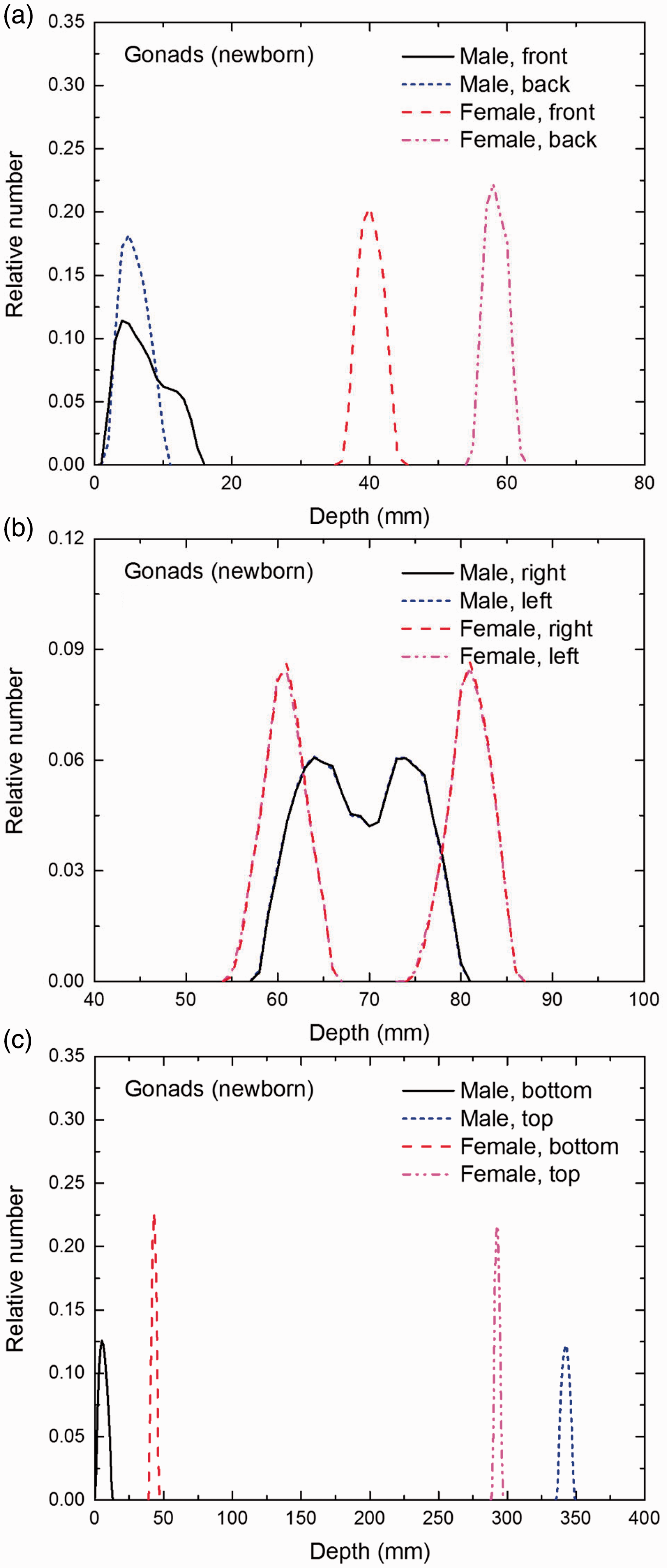
Distribution of depths of 10 million randomly sampled points in the gonads below the body surface of the newborn male/female phantoms at: (a) front and back, (b) right and left, and (c) bottom and top.
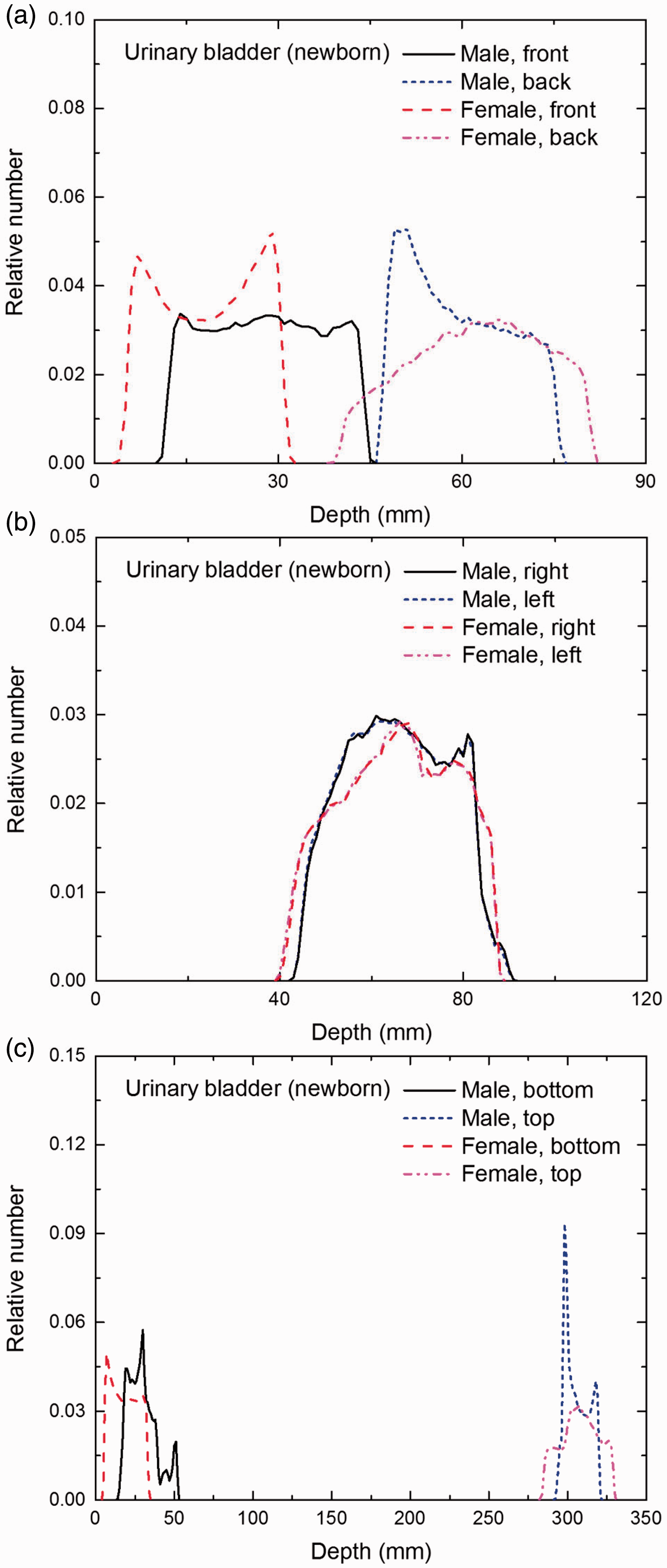
Distribution of depths of 10 million randomly sampled points in the urinary bladder wall below the body surface of the newborn male/female phantoms at: (a) front and back, (b) right and left, and (c) bottom and top.
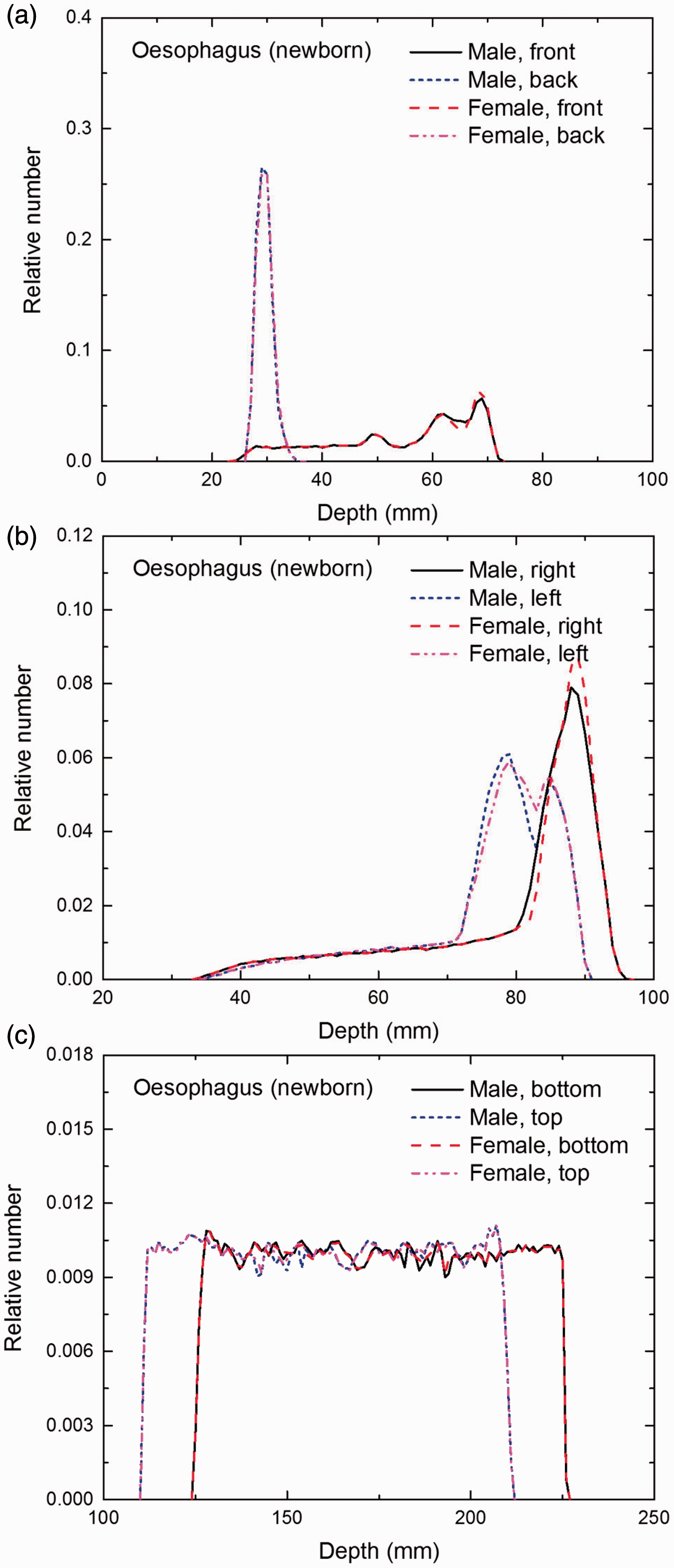
Distribution of depths of 10 million randomly sampled points in the oesophagus wall below the body surface of the newborn male/female phantoms at: (a) front and back, (b) right and left, and (c) bottom and top.
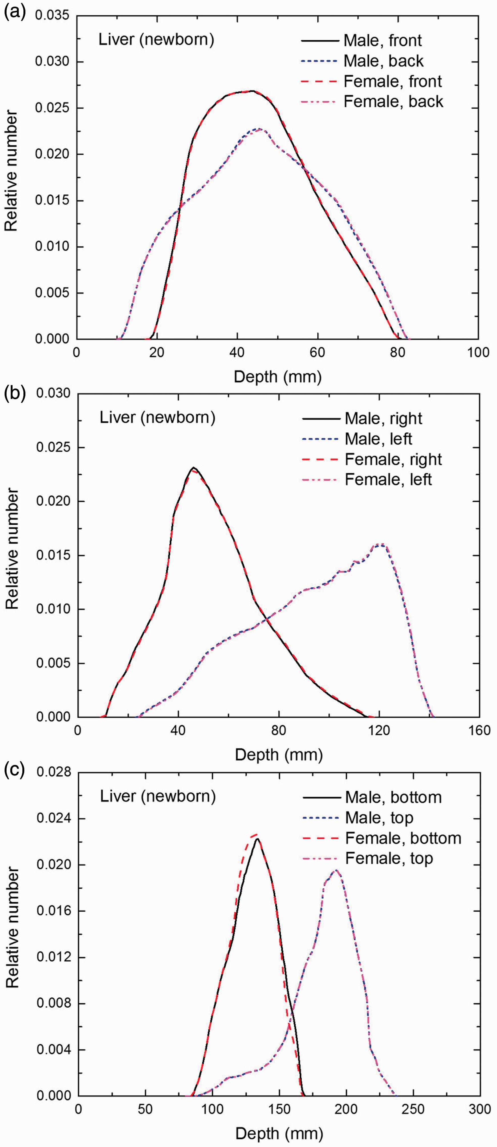
Distribution of depths of 10 million randomly sampled points in the liver below the body surface of the newborn male/female phantoms at: (a) front and back, (b) right and left, and (c) bottom and top.
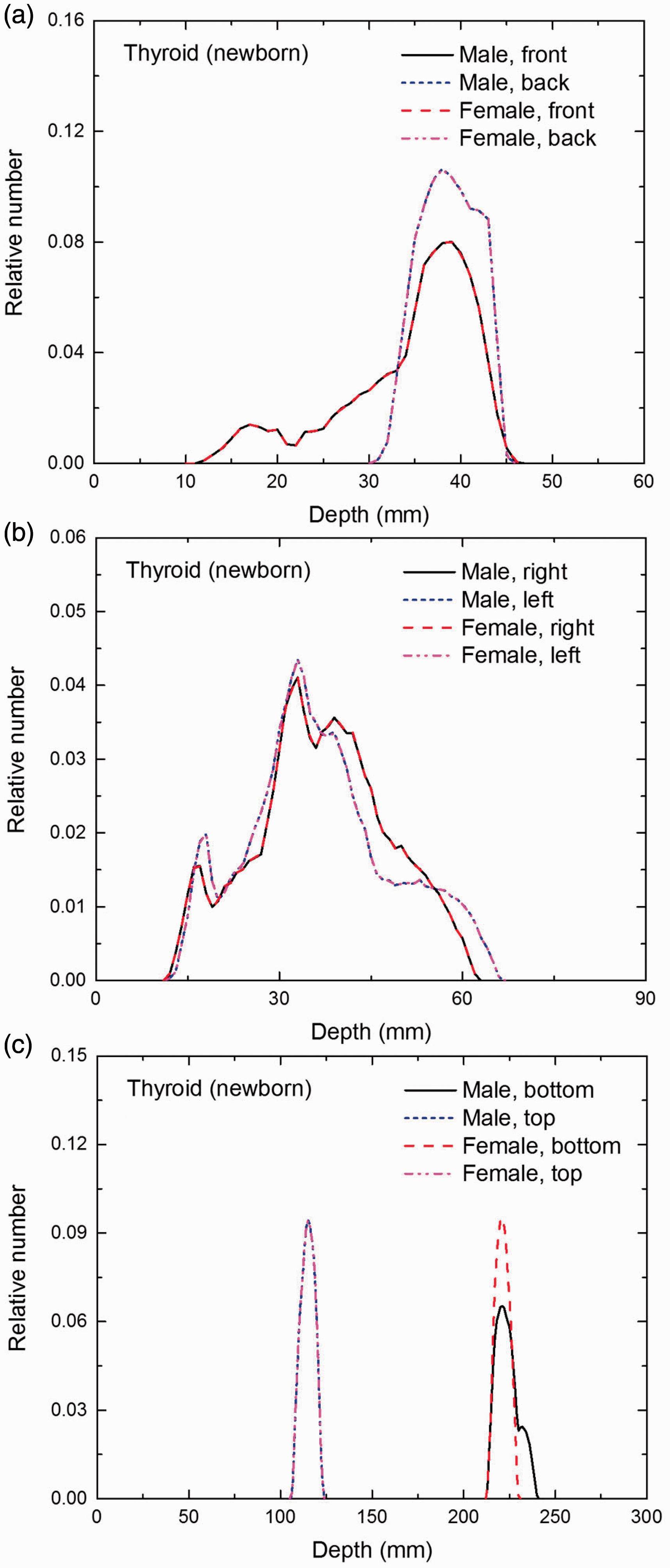
Distribution of depths of 10 million randomly sampled points in the thyroid below the body surface of the newborn male/female phantoms at: (a) front and back, (b) right and left, and (c) bottom and top.
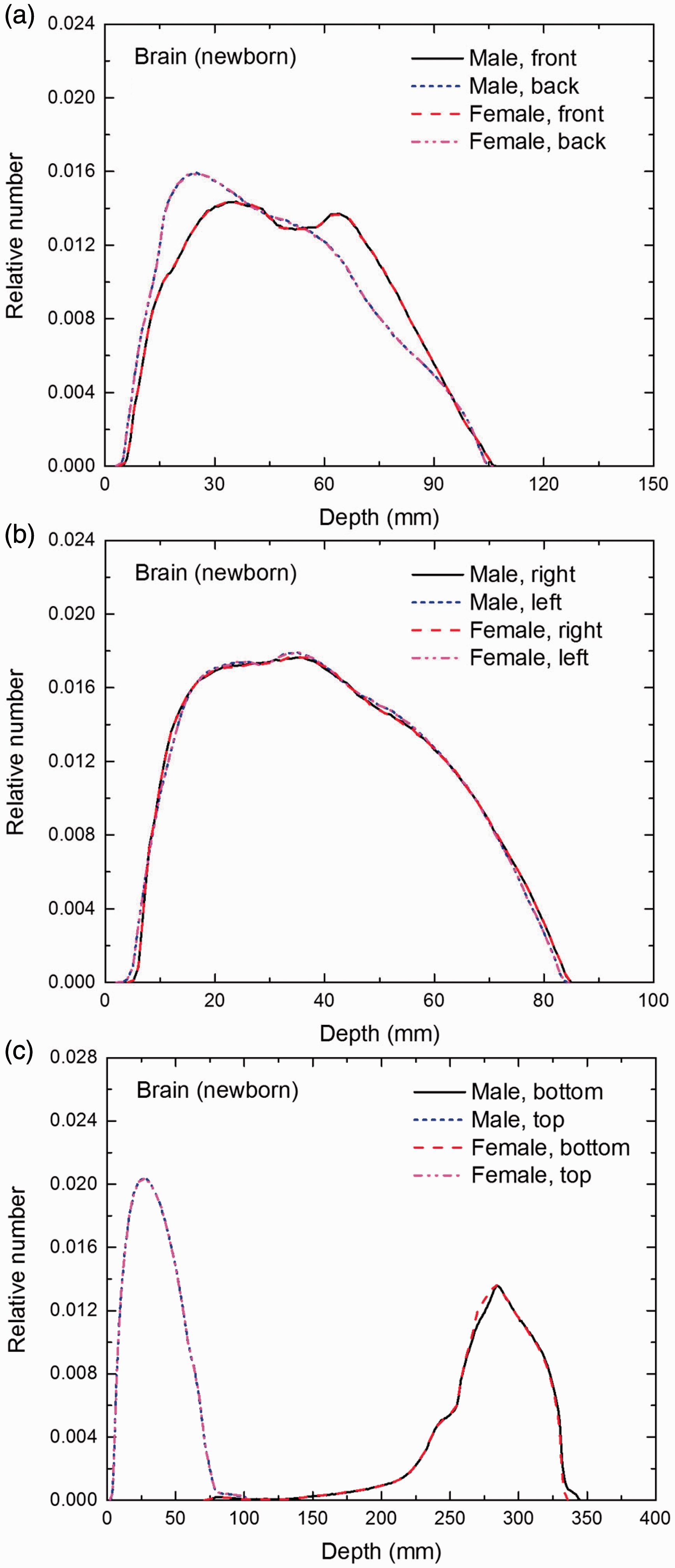
Distribution of depths of 10 million randomly sampled points in the brain below the body surface of the newborn male/female phantoms at: (a) front and back, (b) right and left, and (c) bottom and top.
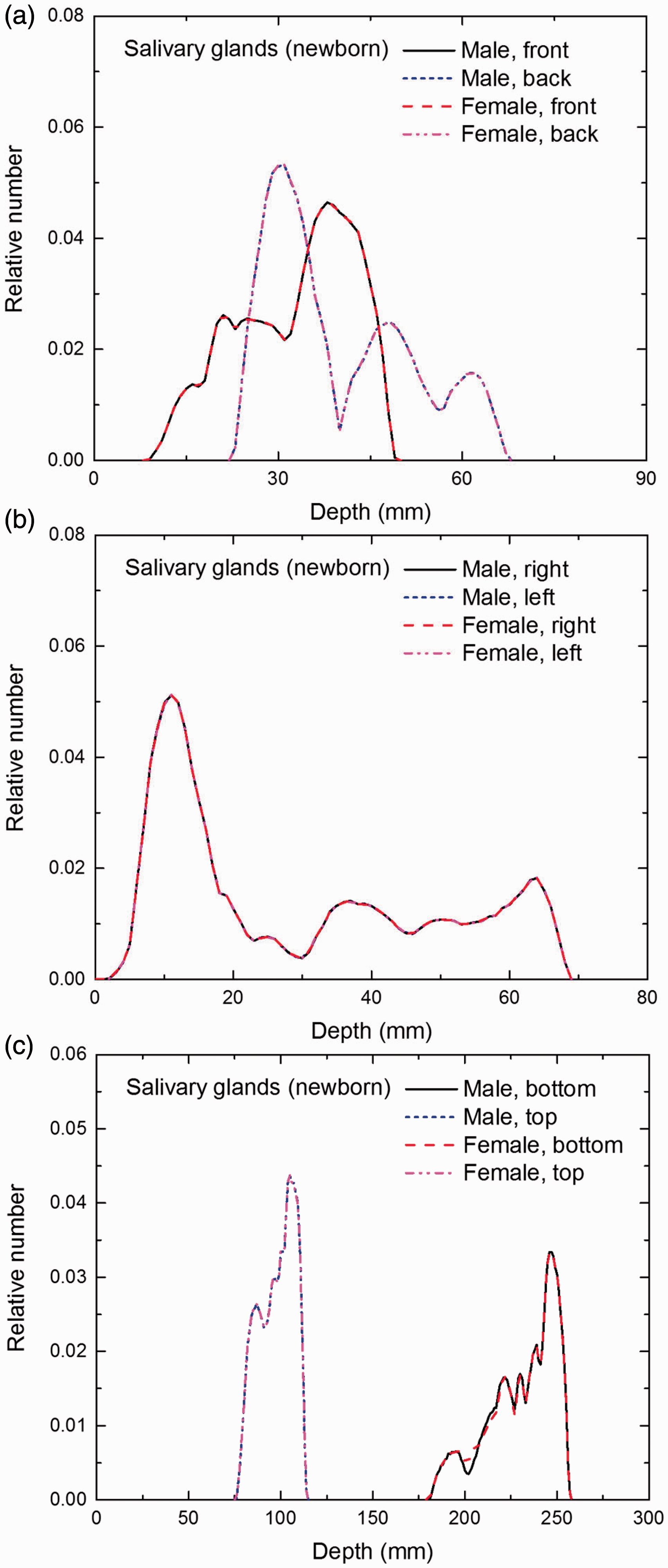
Distribution of depths of 10 million randomly sampled points in the salivary glands below the body surface of the newborn male/female phantoms at: (a) front and back, (b) right and left, and (c) bottom and top.
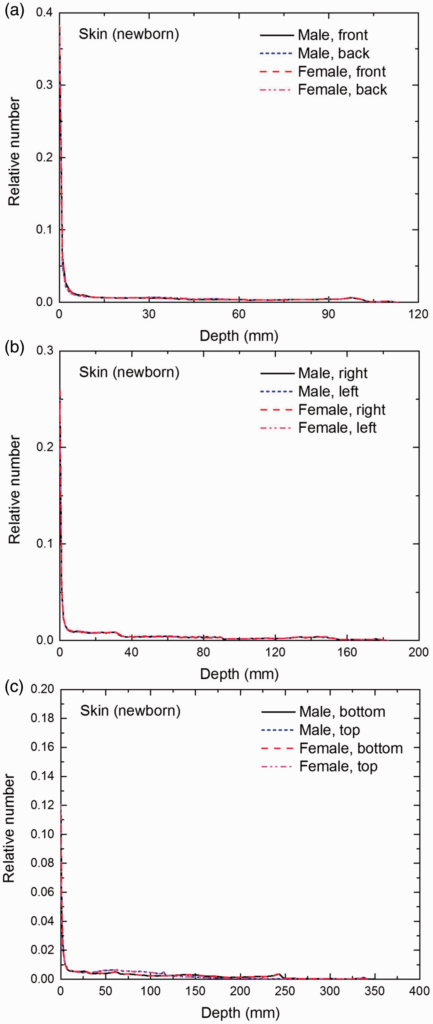
Distribution of depths of 10 million randomly sampled points in the skin below the body surface of the newborn male/female phantoms at: (a) front and back, (b) right and left, and (c) bottom and top.
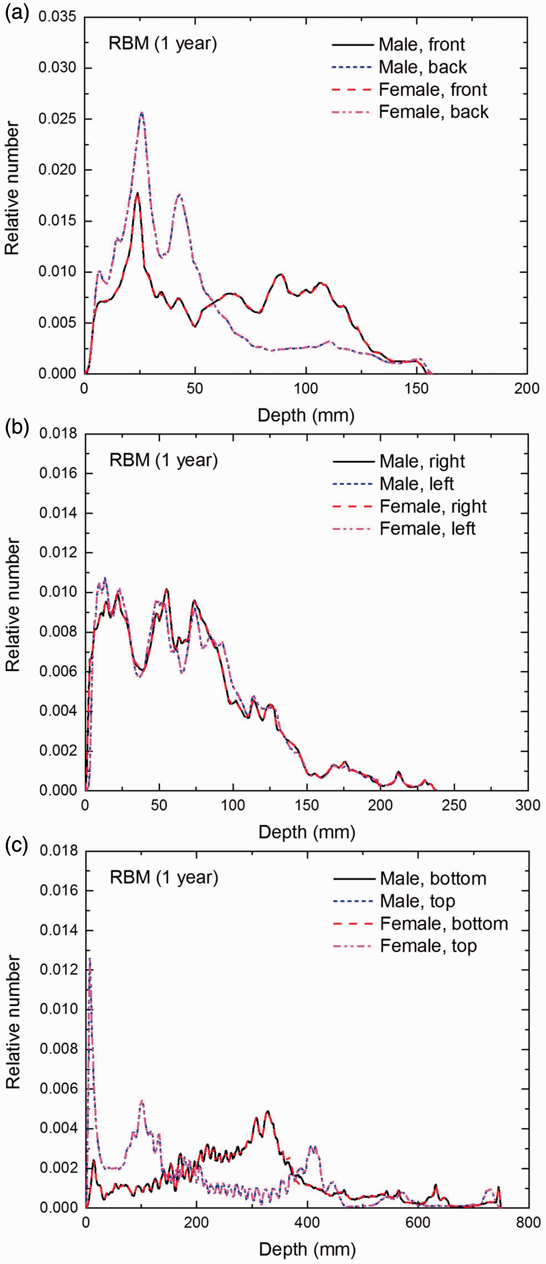
Distribution of depths of 10 million randomly sampled points in the red bone marrow (RBM) below the body surface of the 1-year-old male/female phantoms at: (a) front and back, (b) right and left, and (c) bottom and top.
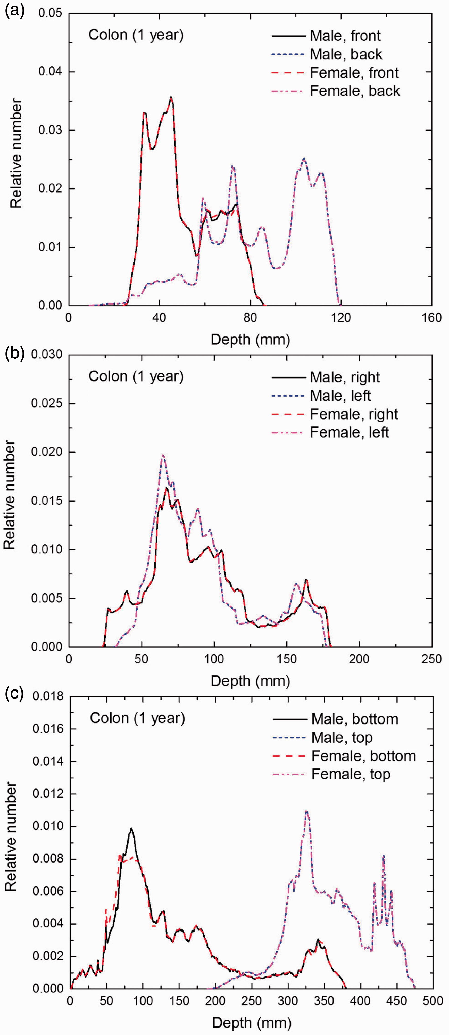
Distribution of depths of 10 million randomly sampled points in the colon wall below the body surface of the 1-year-old male/female phantoms at: (a) front and back, (b) right and left, and (c) bottom and top.
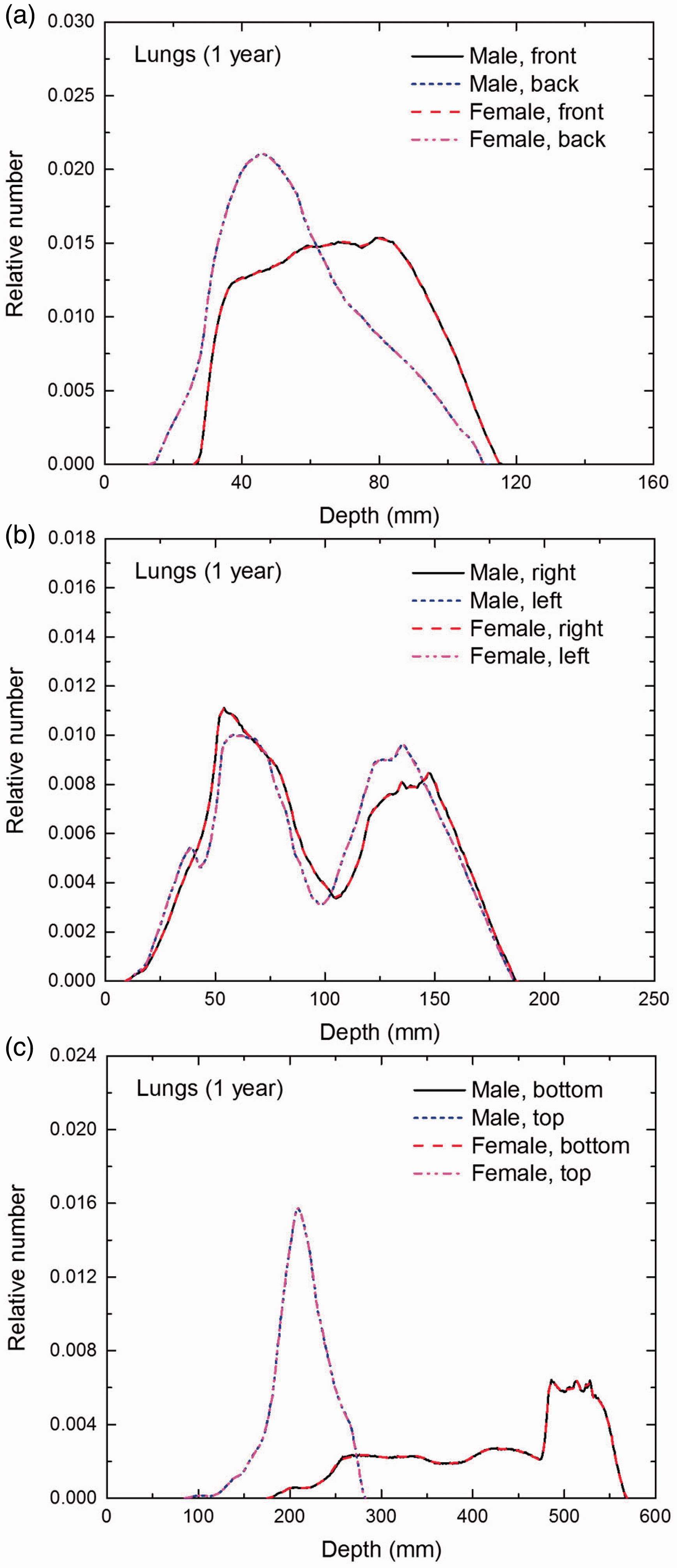
Distribution of depths of 10 million randomly sampled points in the lungs below the body surface of the 1-year-old male/female phantoms at: (a) front and back, (b) right and left, and (c) bottom and top.
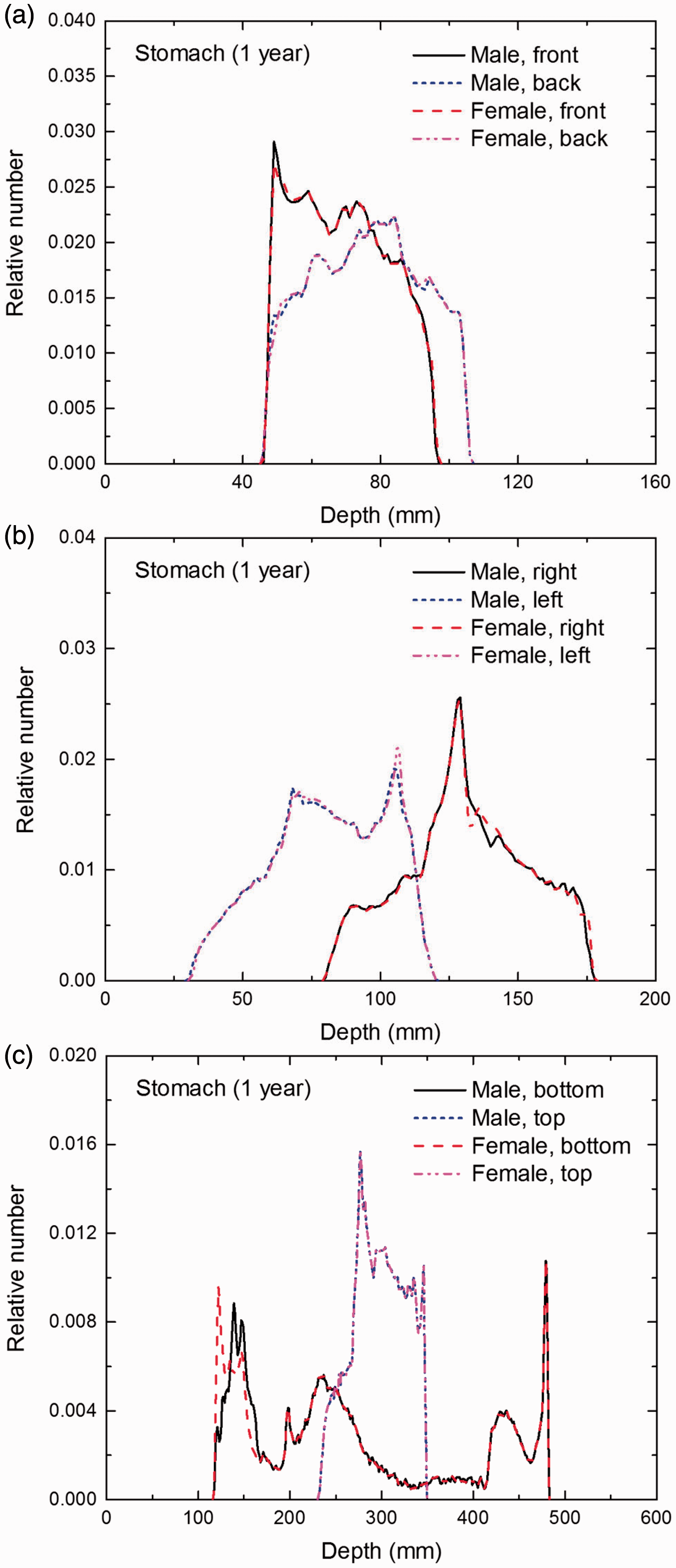
Distribution of depths of 10 million randomly sampled points in the stomach wall below the body surface of the 1-year-old male/female phantoms at: (a) front and back, (b) right and left, and (c) bottom and top.
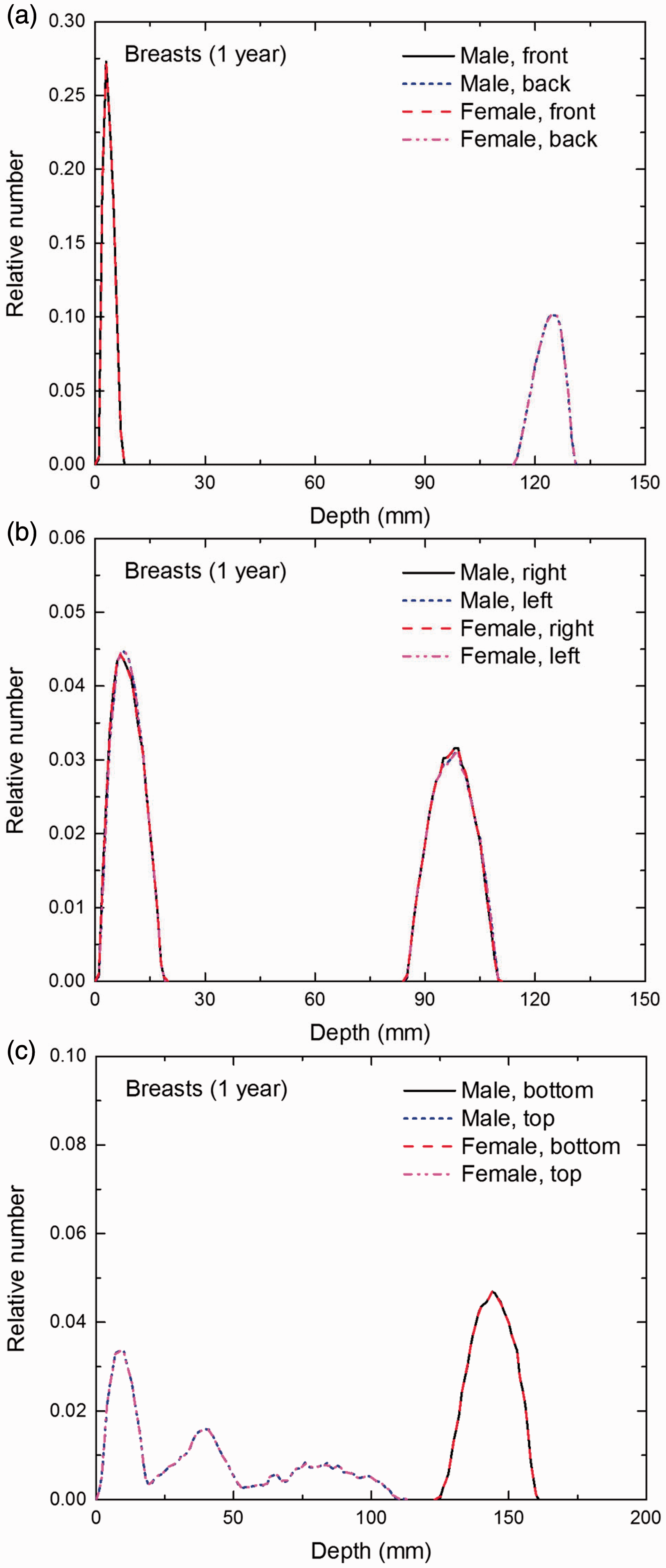
Distribution of depths of 10 million randomly sampled points in the breasts below the body surface of the 1-year-old male/female phantoms at: (a) front and back, (b) right and left, and (c) bottom and top.
Distribution of depths of 10 million randomly sampled points in the gonads below the body surface of the 1-year-old male/female phantoms at: (a) front and back, (b) right and left, and (c) bottom and top.
Distribution of depths of 10 million randomly sampled points in the urinary bladder wall below the body surface of the 1-year-old male/female phantoms at: (a) front and back, (b) right and left, and (c) bottom and top.
Distribution of depths of 10 million randomly sampled points in the oesophagus wall below the body surface of the 1-year-old male/female phantoms at: (a) front and back, (b) right and left, and (c) bottom and top.
Distribution of depths of 10 million randomly sampled points in the liver below the body surface of the 1-year-old male/female phantoms at: (a) front and back, (b) right and left, and (c) bottom and top.
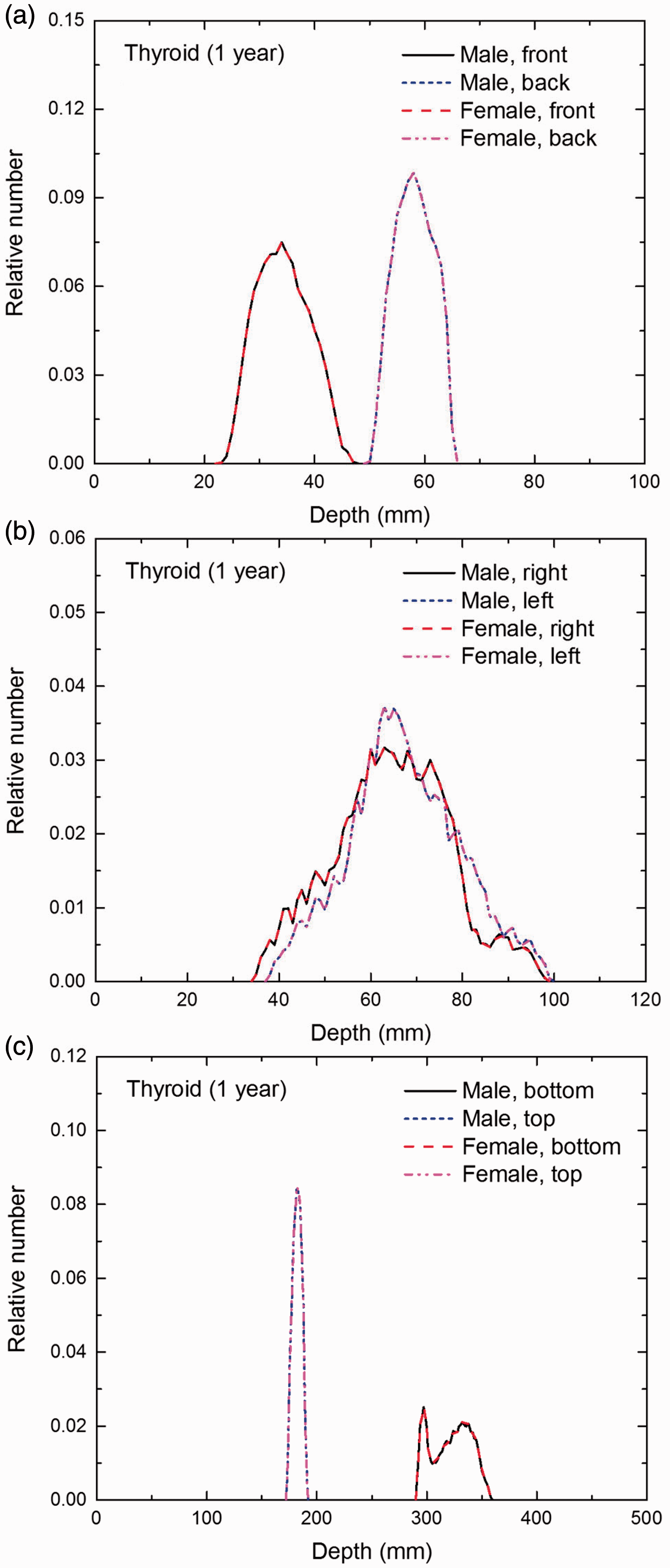
Distribution of depths of 10 million randomly sampled points in the thyroid below the body surface of the 1-year-old male/female phantoms at: (a) front and back, (b) right and left, and (c) bottom and top.
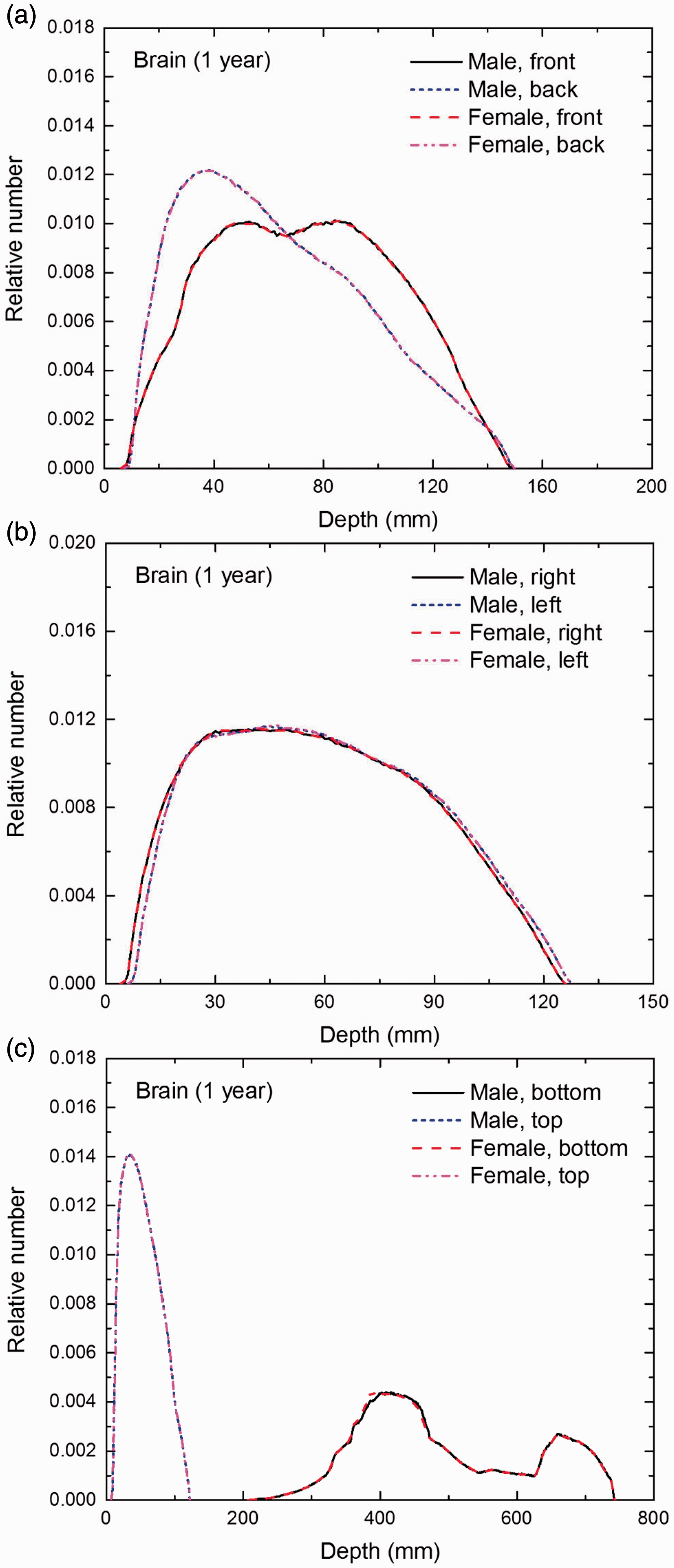
Distribution of depths of 10 million randomly sampled points in the brain below the body surface of the 1-year-old male/female phantoms at: (a) front and back, (b) right and left, and (c) bottom and top.
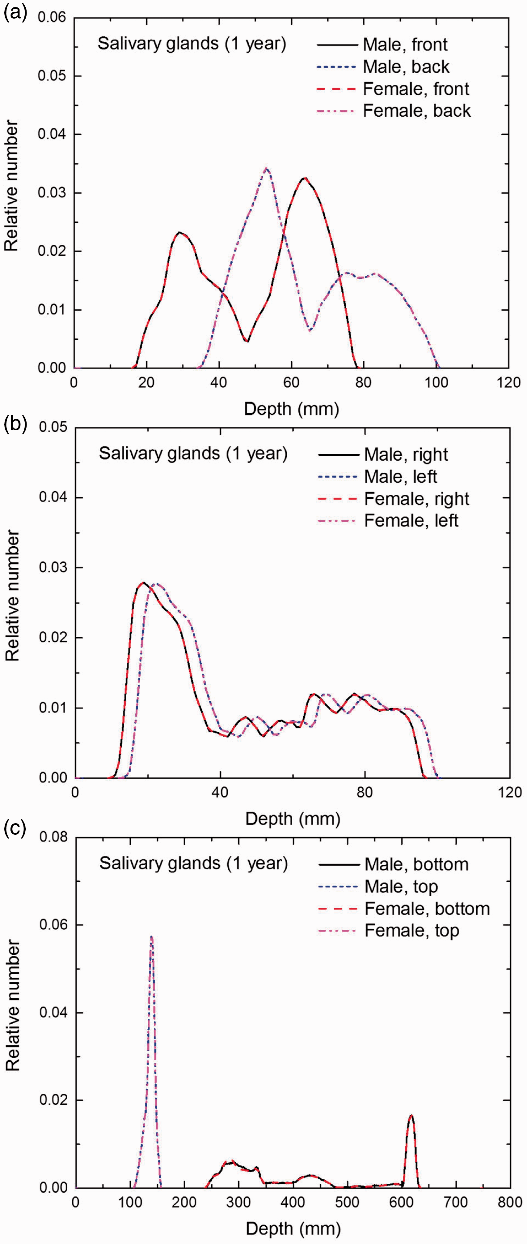
Distribution of depths of 10 million randomly sampled points in the salivary glands below the body surface of the 1-year-old male/female phantoms at: (a) front and back, (b) right and left, and (c) bottom and top.
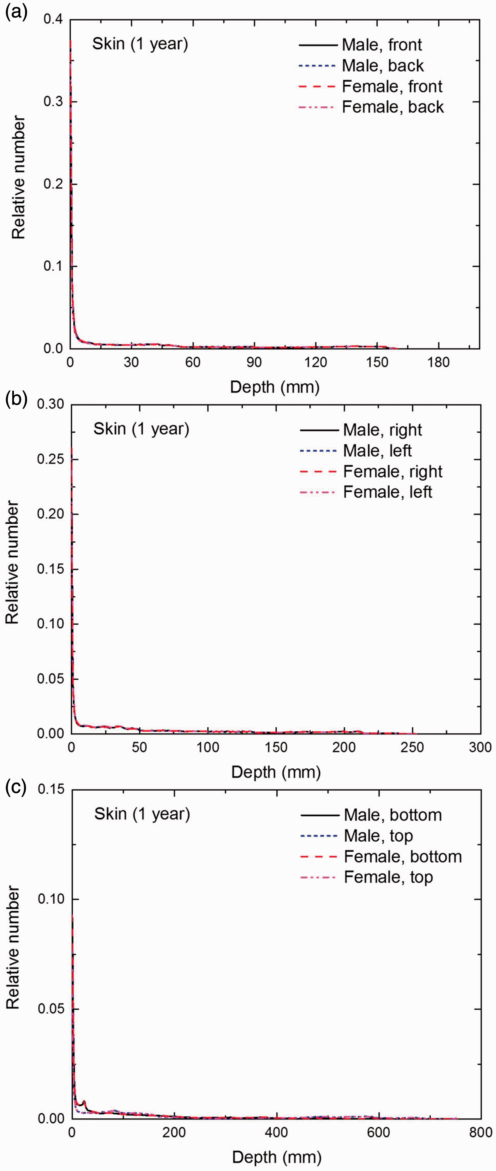
Distribution of depths of 10 million randomly sampled points in the skin below the body surface of the 1-year-old male/female phantoms at: (a) front and back, (b) right and left, and (c) bottom and top.
Distribution of depths of 10 million randomly sampled points in the red bone marrow (RBM) below the body surface of the 5-year-old male/female phantoms at: (a) front and back, (b) right and left, and (c) bottom and top.
Distribution of depths of 10 million randomly sampled points in the colon wall below the body surface of the 5-year-old male/female phantoms at: (a) front and back, (b) right and left, and (c) bottom and top.
Distribution of depths of 10 million randomly sampled points in the lungs below the body surface of the 5-year-old male/female phantoms at: (a) front and back, (b) right and left, and (c) bottom and top.
Distribution of depths of 10 million randomly sampled points in the stomach wall below the body surface of the 5-year-old male/female phantoms at: (a) front and back, (b) right and left, and (c) bottom and top.
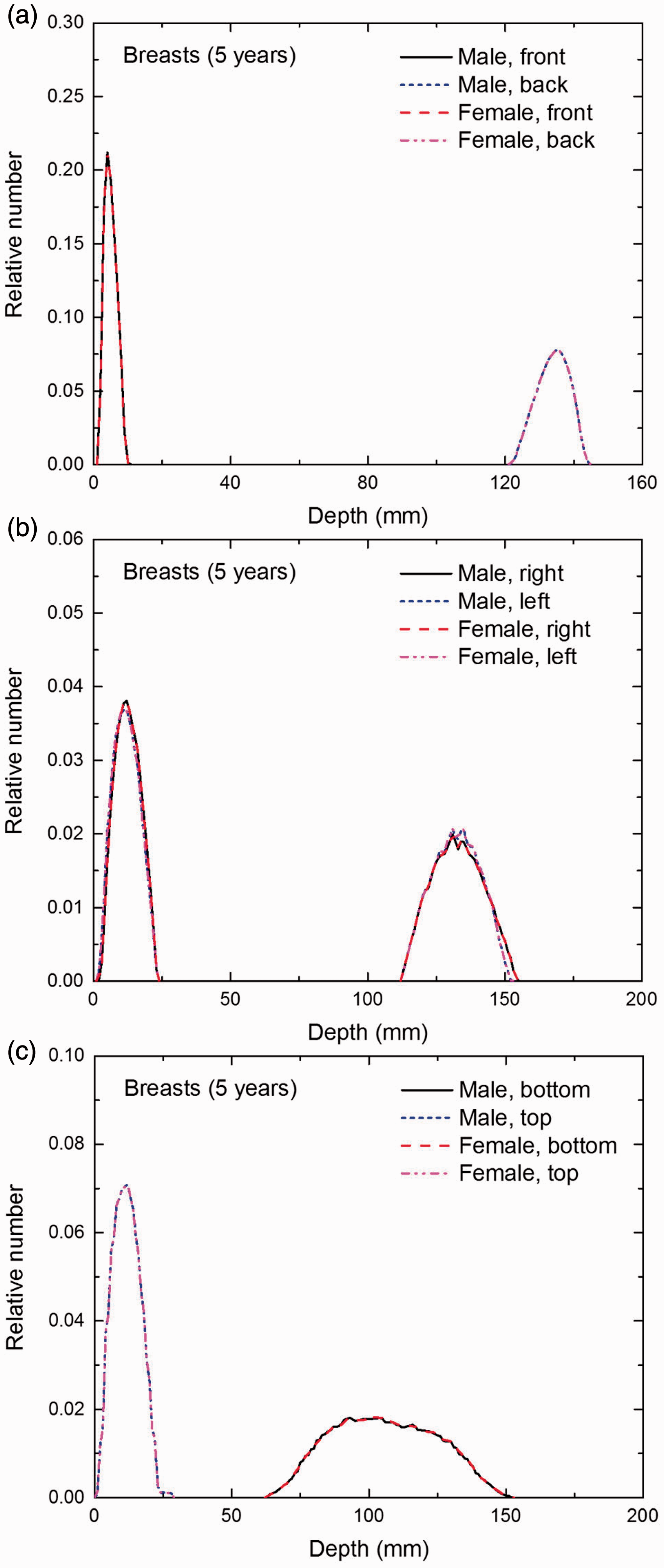
Distribution of depths of 10 million randomly sampled points in the breasts below the body surface of the 5-year-old male/female phantoms at: (a) front and back, (b) right and left, and (c) bottom and top.
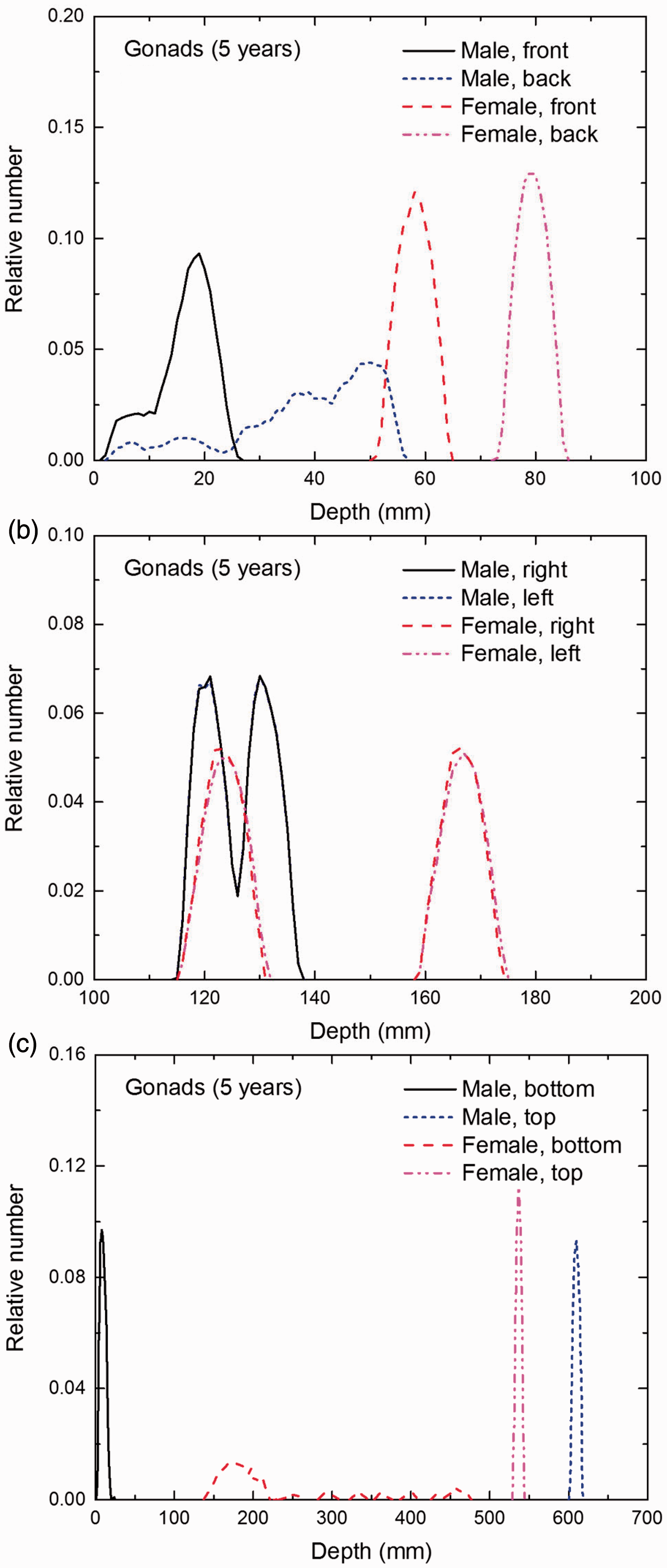
Distribution of depths of 10 million randomly sampled points in the gonads below the body surface of the 5-year-old male/female phantoms at: (a) front and back, (b) right and left, and (c) bottom and top.
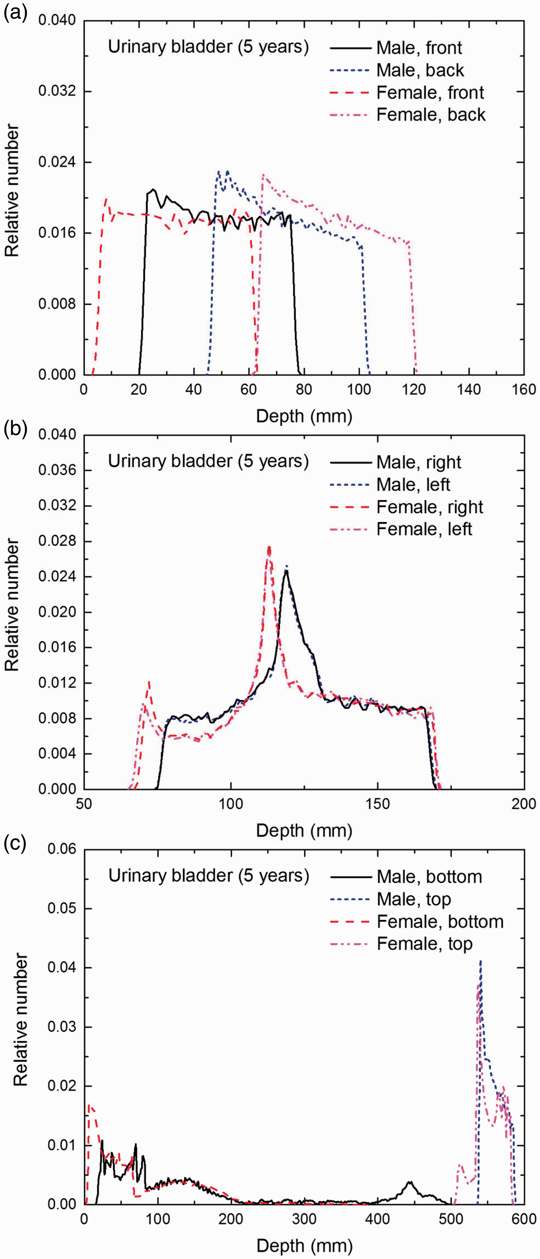
Distribution of depths of 10 million randomly sampled points in the urinary bladder wall below the body surface of the 5-year-old male/female phantoms at: (a) front and back, (b) right and left, and (c) bottom and top.
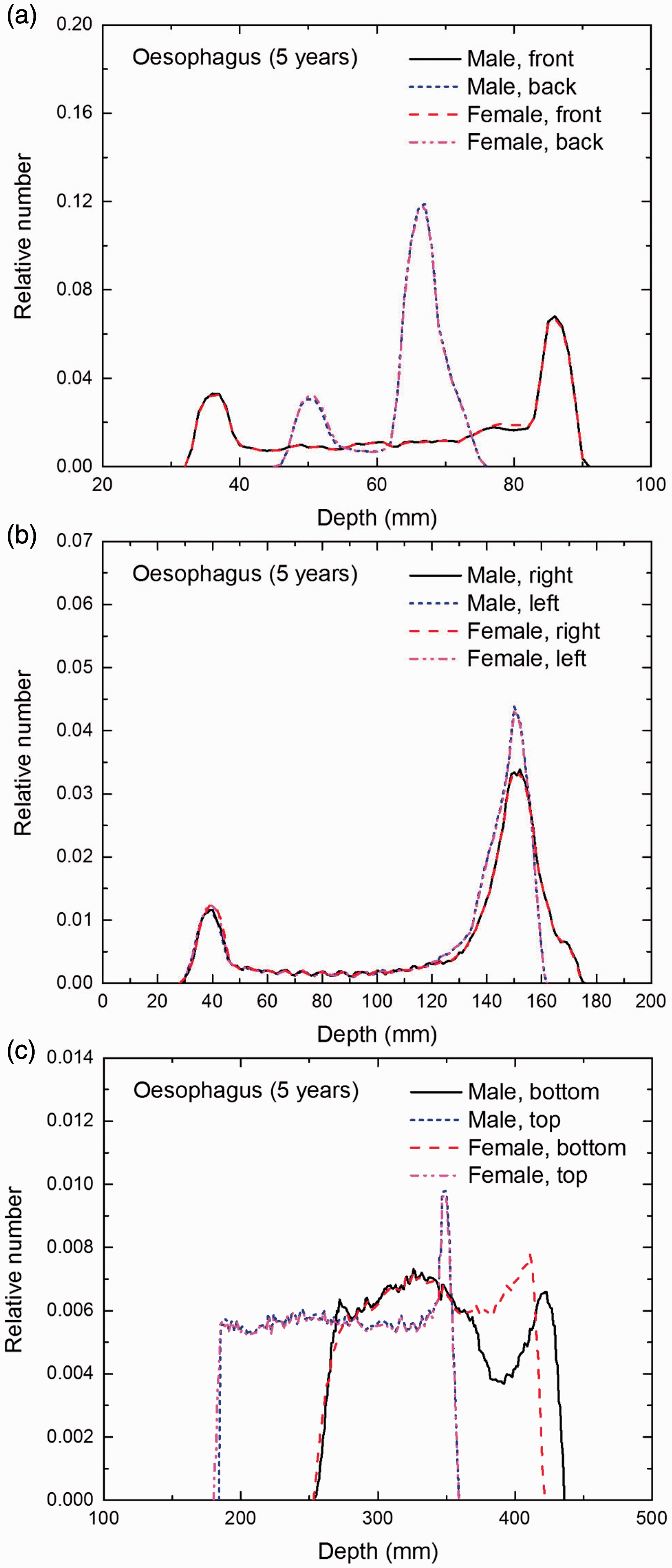
Distribution of depths of 10 million randomly sampled points in the oesophagus wall below the body surface of the 5-year-old male/female phantoms at: (a) front and back, (b) right and left, and (c) bottom and top.
Distribution of depths of 10 million randomly sampled points in the liver below the body surface of the 5-year-old male/female phantoms at: (a) front and back, (b) right and left, and (c) bottom and top.
Distribution of depths of 10 million randomly sampled points in the thyroid below the body surface of the 5-year-old male/female phantoms at: (a) front and back, (b) right and left, and (c) bottom and top.
Distribution of depths of 10 million randomly sampled points in the brain below the body surface of the 5-year-old male/female phantoms at: (a) front and back, (b) right and left, and (c) bottom and top.
Distribution of depths of 10 million randomly sampled points in the salivary glands below the body surface of the 5-year-old male/female phantoms at: (a) front and back, (b) right and left, and (c) bottom and top.
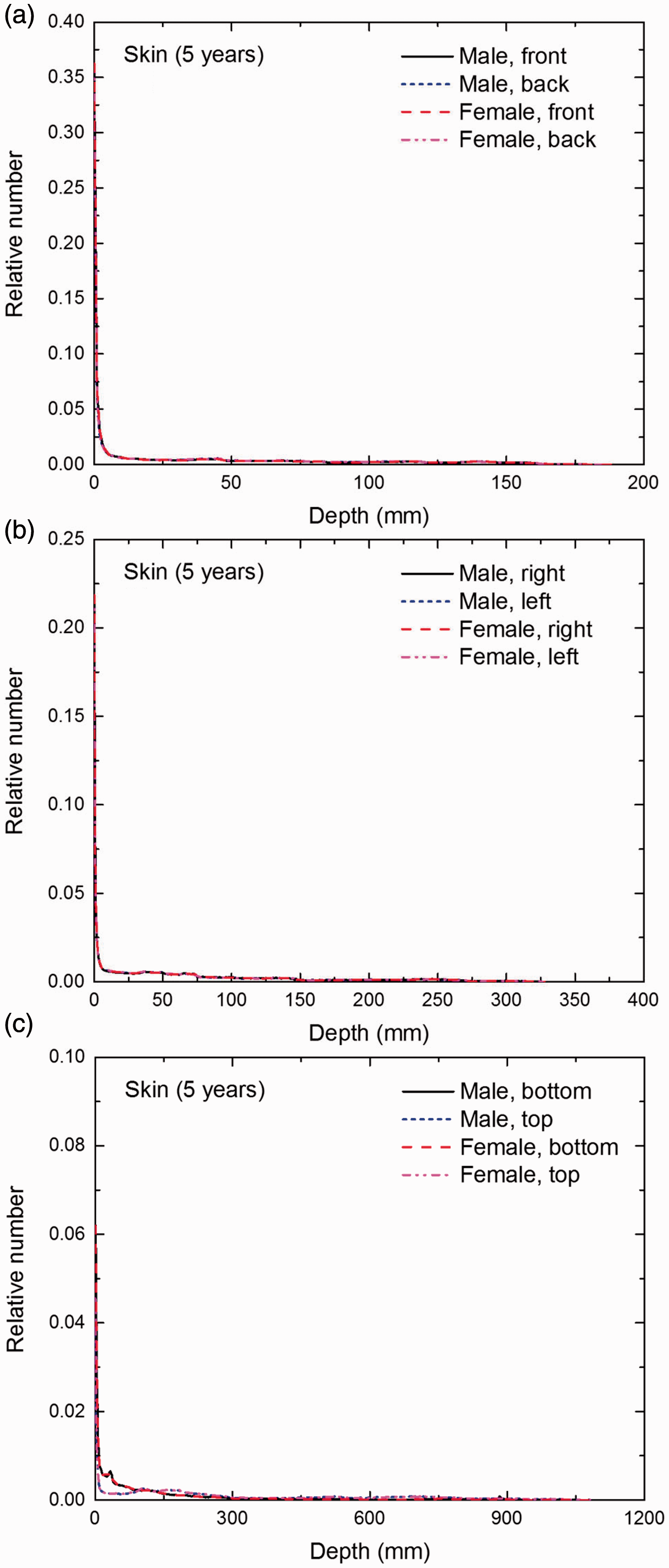
Distribution of depths of 10 million randomly sampled points in the skin below the body surface of the 5-year-old male/female phantoms at: (a) front and back, (b) right and left, and (c) bottom and top.
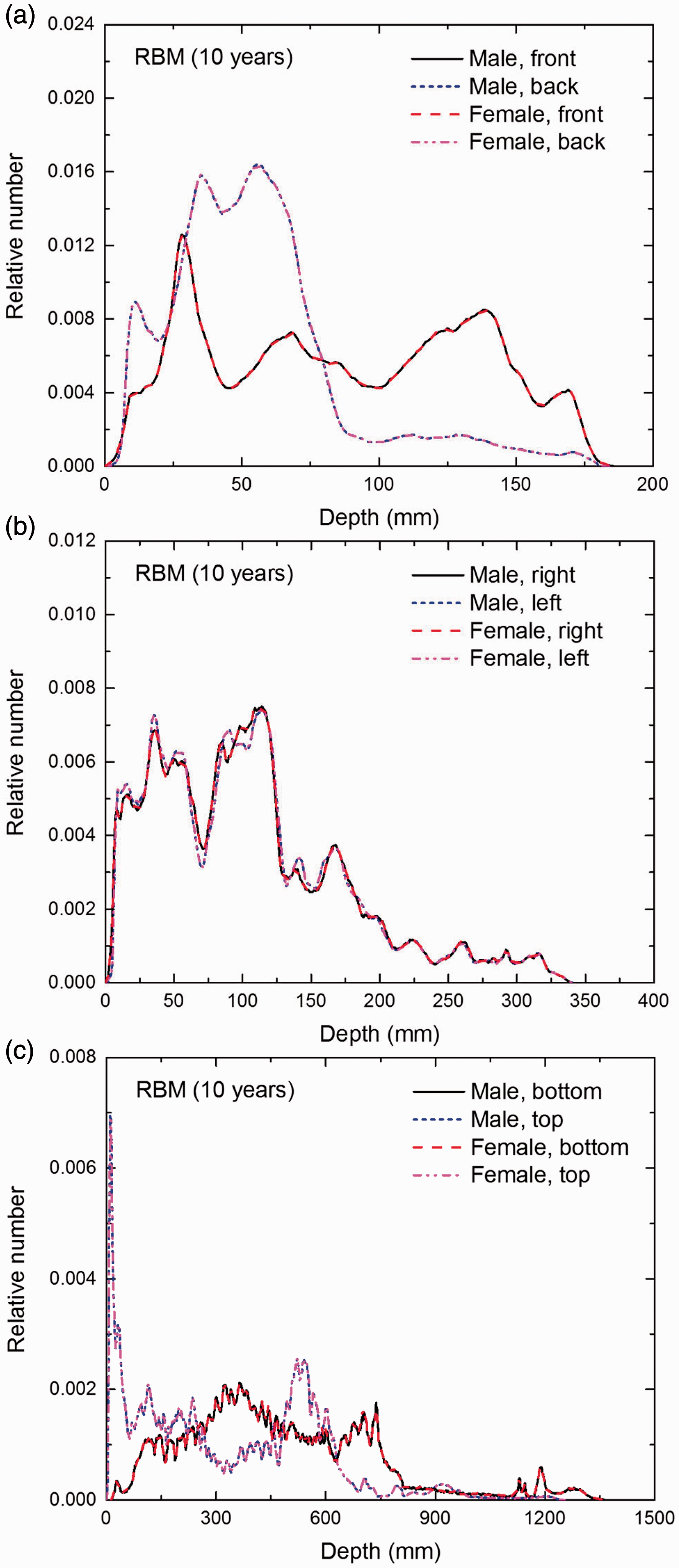
Distribution of depths of 10 million randomly sampled points in the red bone marrow (RBM) below the body surface of the 10-year-old male/female phantoms at: (a) front and back, (b) right and left, and (c) bottom and top.
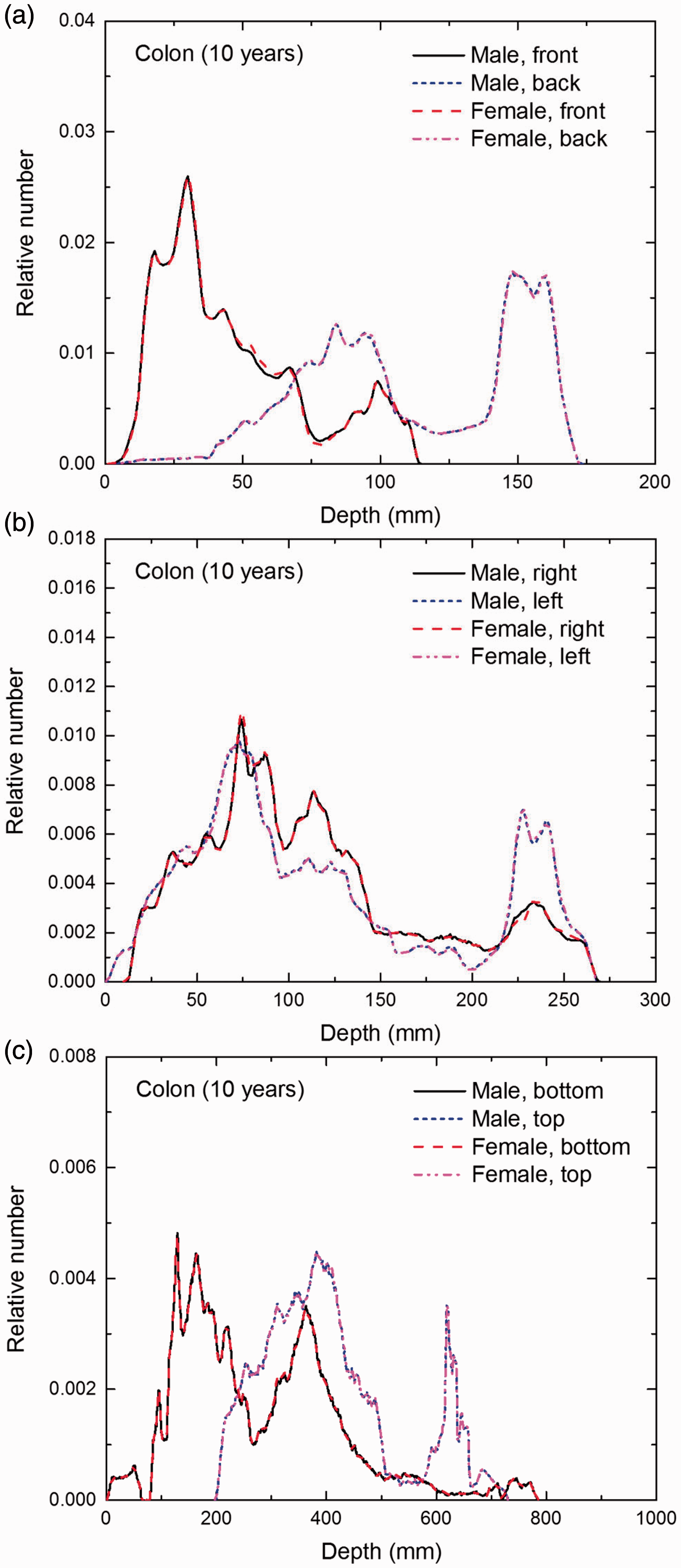
Distribution of depths of 10 million randomly sampled points in the colon wall below the body surface of the 10-year-old male/female phantoms at: (a) front and back, (b) right and left, and (c) bottom and top.
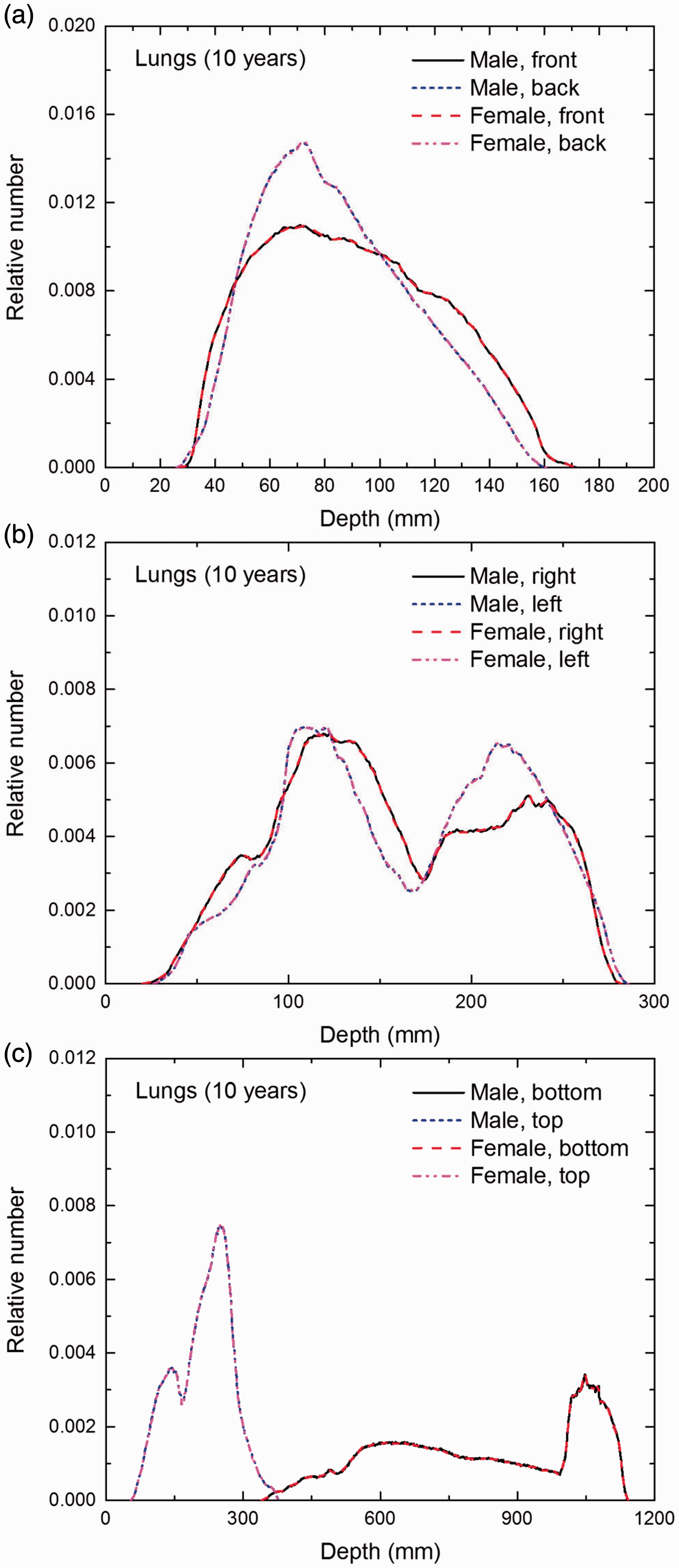
Distribution of depths of 10 million randomly sampled points in the lungs below the body surface of the 10-year-old male/female phantoms at: (a) front and back, (b) right and left, and (c) bottom and top.
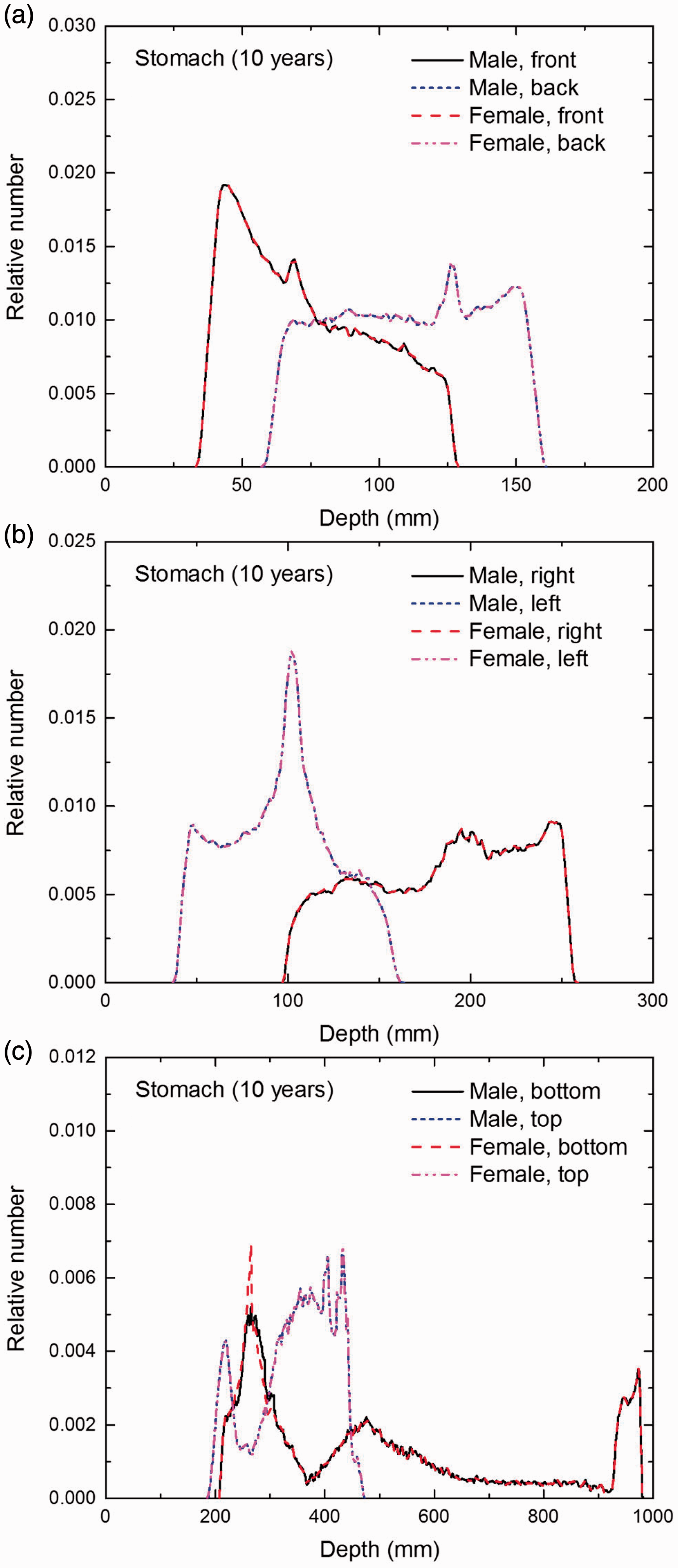
Distribution of depths of 10 million randomly sampled points in the stomach wall below the body surface of the 10-year-old male/female phantoms at: (a) front and back, (b) right and left, and (c) bottom and top.
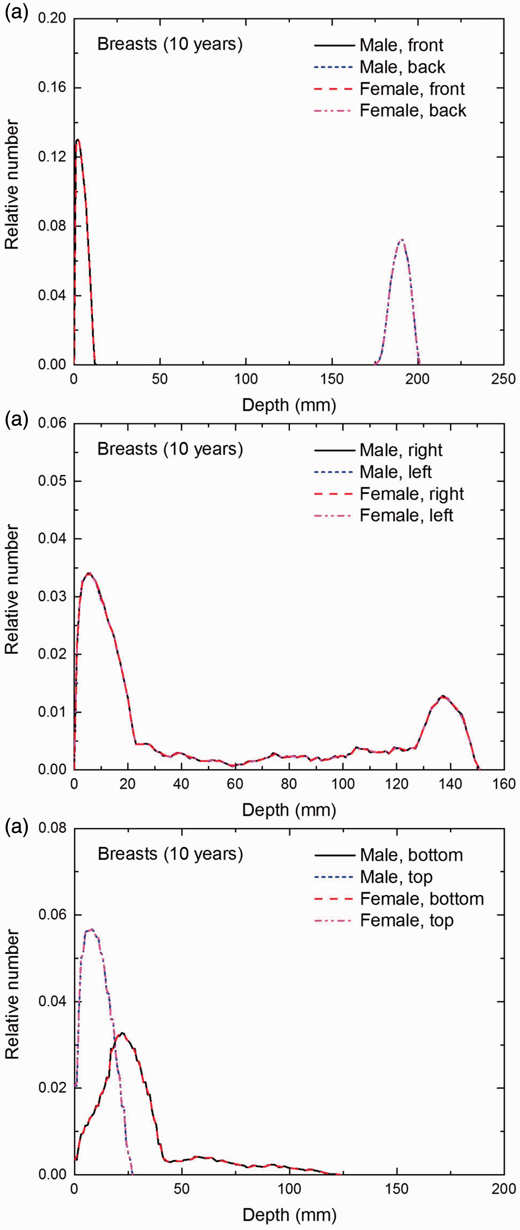
Distribution of depths of 10 million randomly sampled points in the breasts below the body surface of the 10-year-old male/female phantoms at: (a) front and back, (b) right and left, and (c) bottom and top.
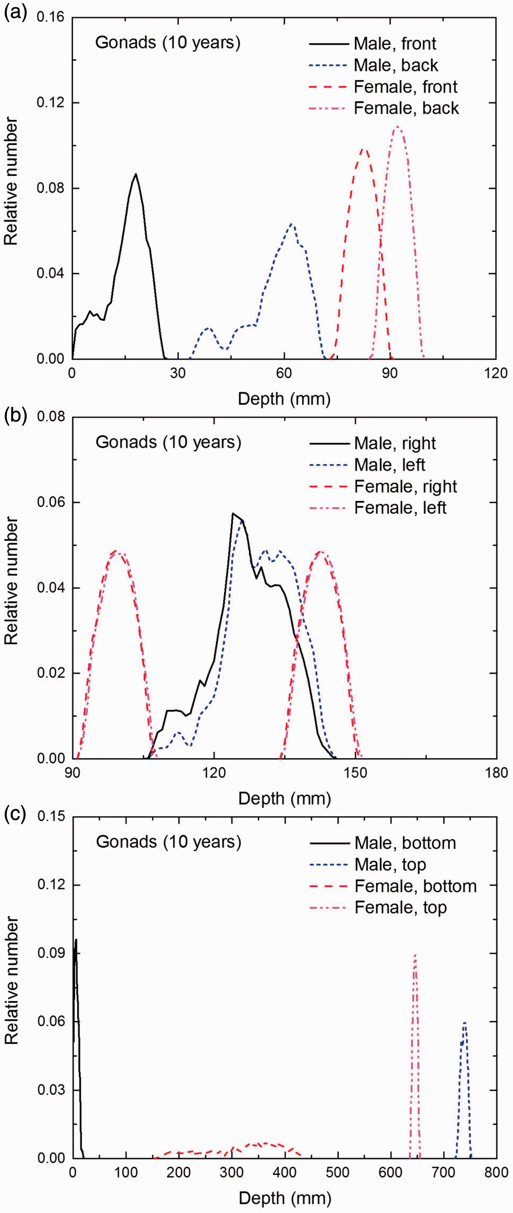
Distribution of depths of 10 million randomly sampled points in the gonads below the body surface of the 10-year-old male/female phantoms at: (a) front and back, (b) right and left, and (c) bottom and top.
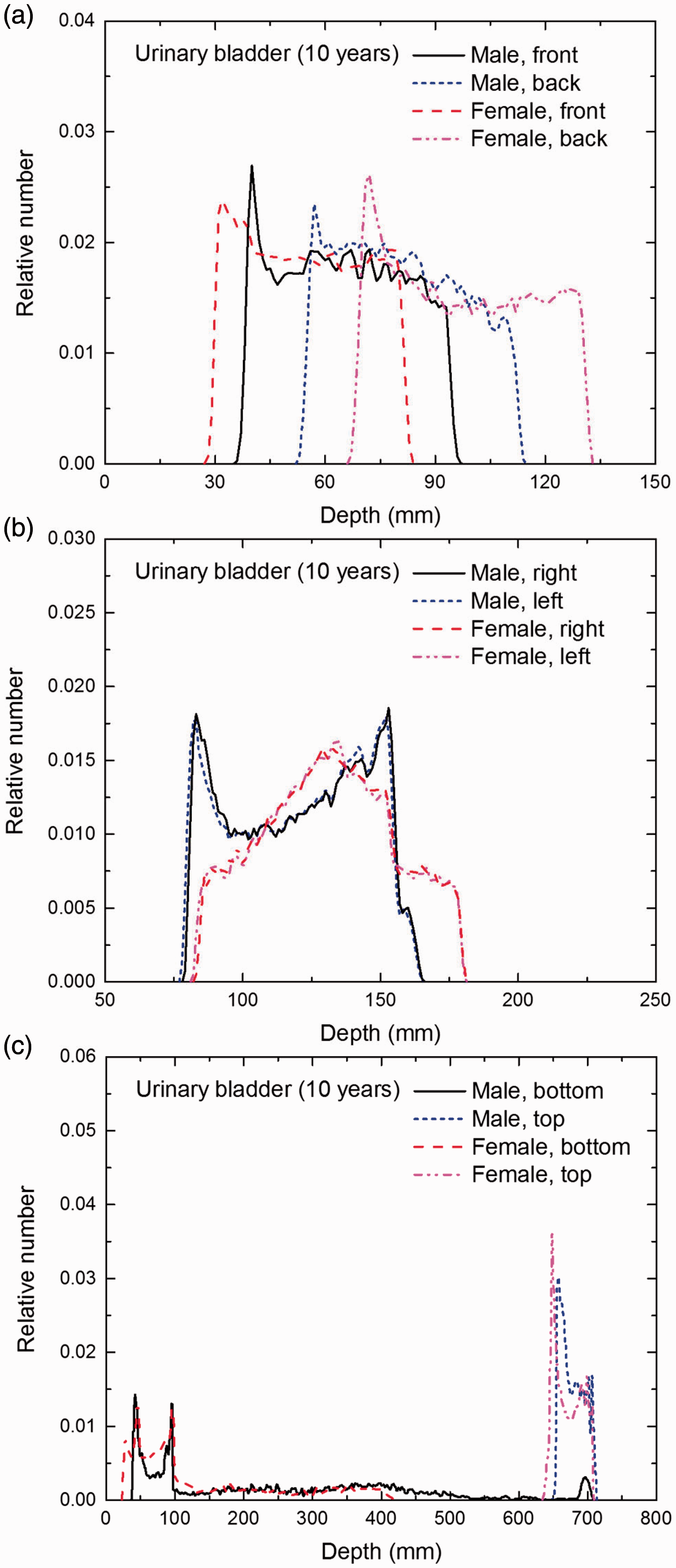
Distribution of depths of 10 million randomly sampled points in the urinary bladder wall below the body surface of the 10-year-old male/female phantoms at: (a) front and back, (b) right and left, and (c) bottom and top.
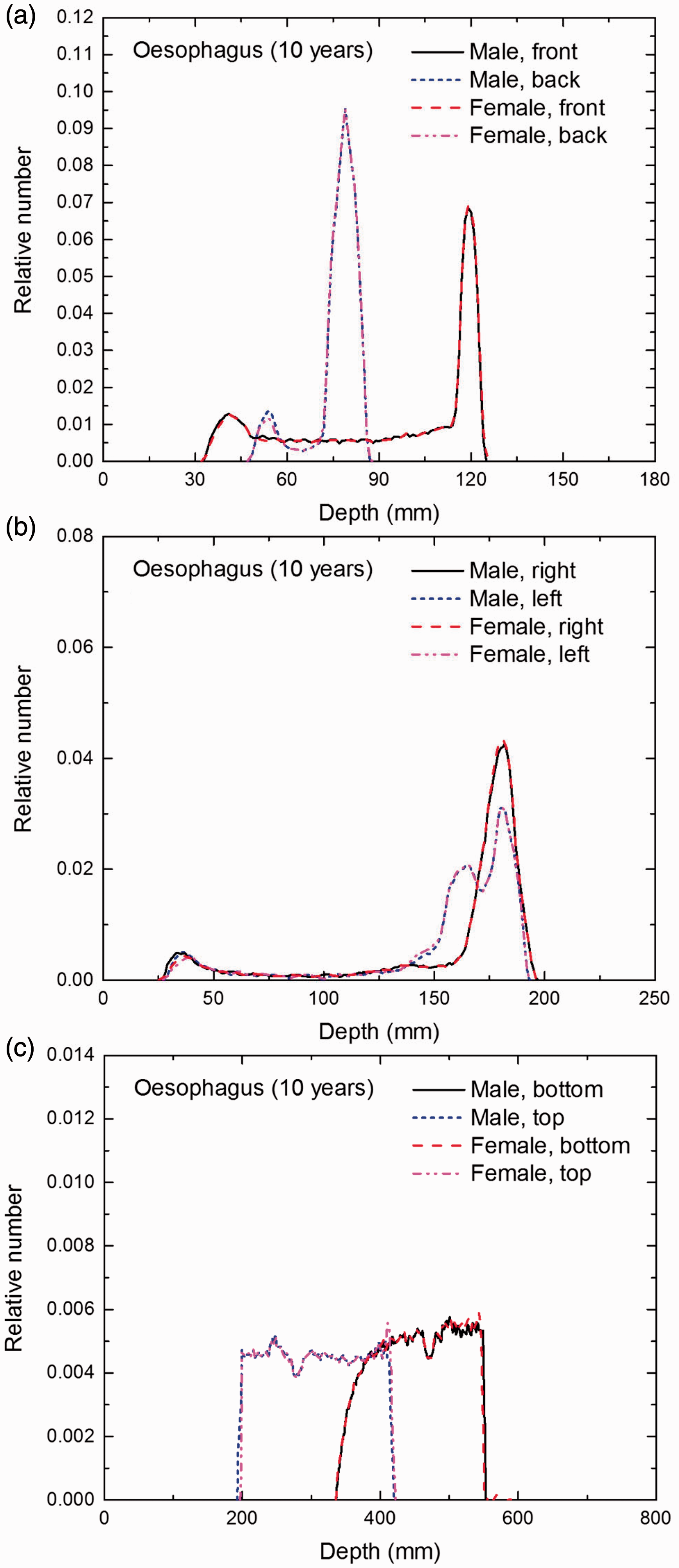
Distribution of depths of 10 million randomly sampled points in the oesophagus wall below the body surface of the 10-year-old male/female phantoms at: (a) front and back, (b) right and left, and (c) bottom and top.
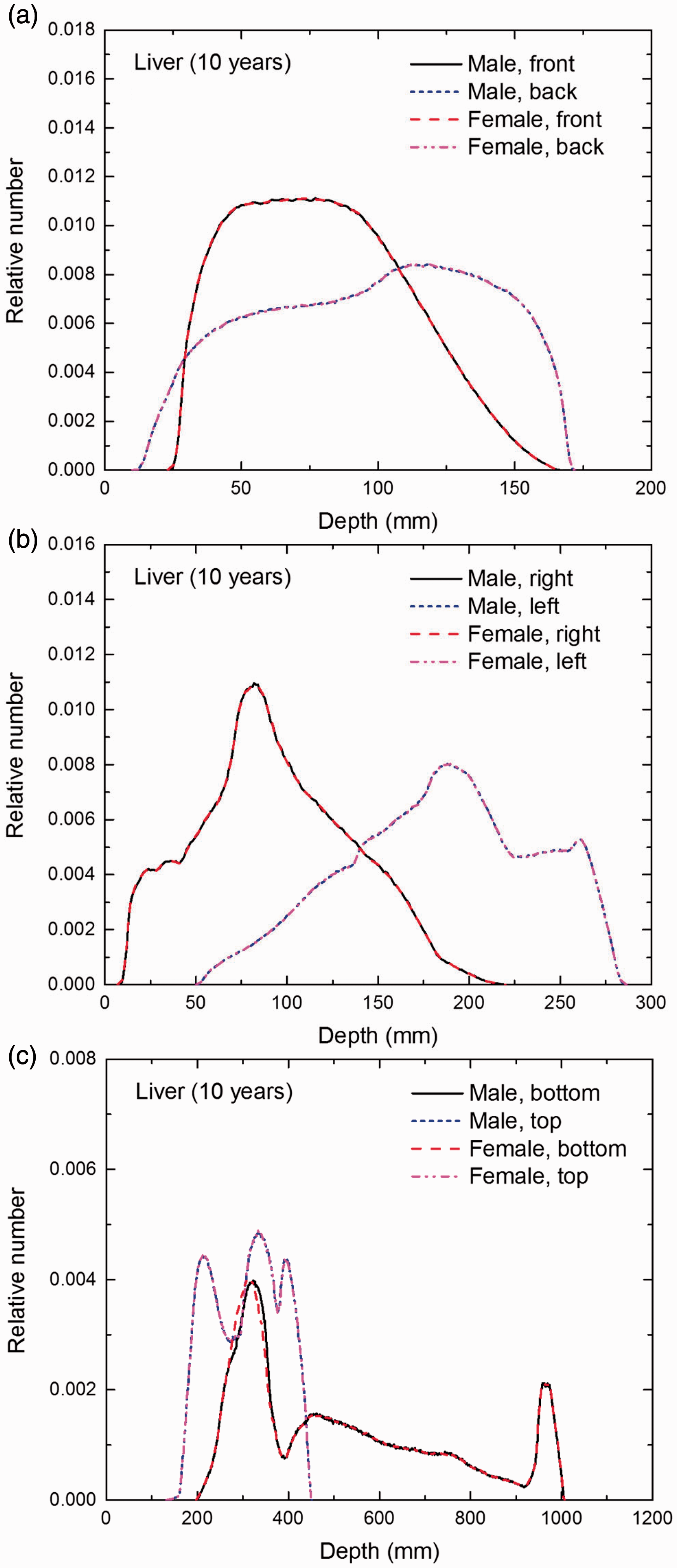
Distribution of depths of 10 million randomly sampled points in the liver below the body surface of the 10-year-old male/female phantoms at: (a) front and back, (b) right and left, and (c) bottom and top.
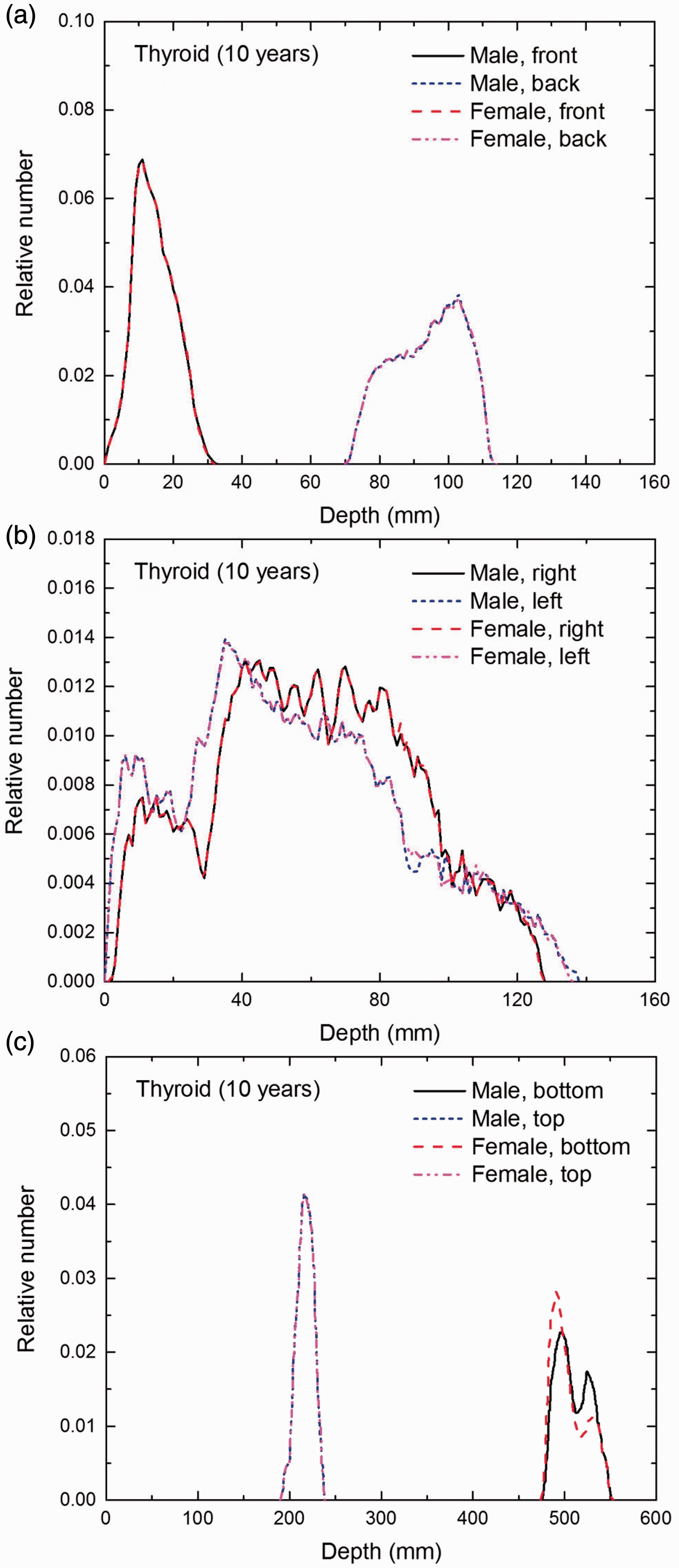
Distribution of depths of 10 million randomly sampled points in the thyroid below the body surface of the 10-year-old male/female phantoms at: (a) front and back, (b) right and left, and (c) bottom and top.
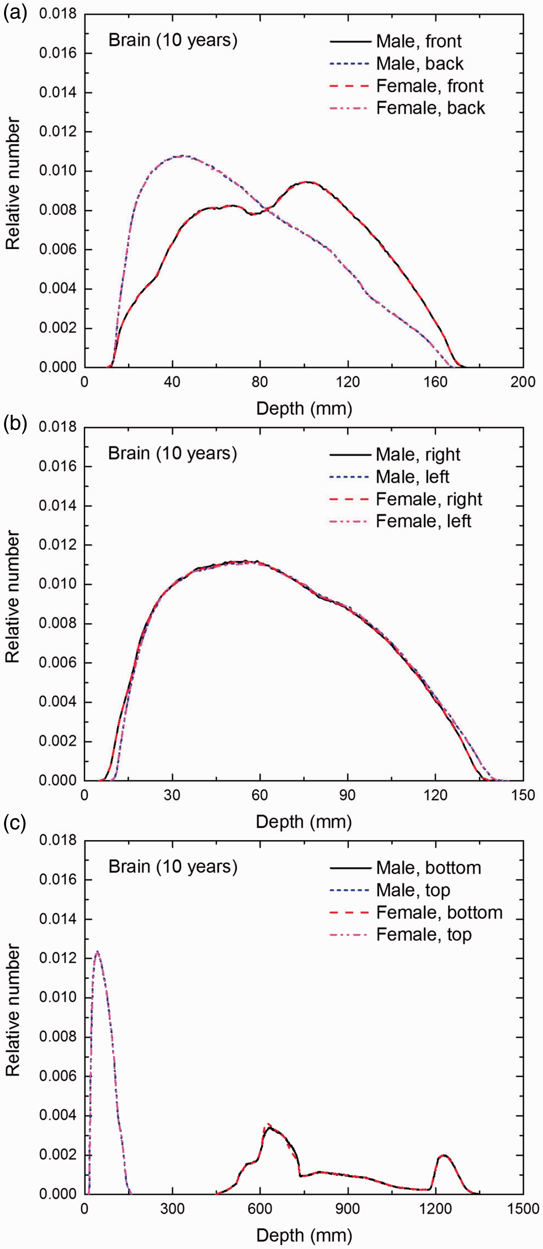
Distribution of depths of 10 million randomly sampled points in the brain below the body surface of the 10-year-old male/female phantoms at: (a) front and back, (b) right and left, and (c) bottom and top.
Distribution of depths of 10 million randomly sampled points in the salivary glands below the body surface of the 10-year-old male/female phantoms at: (a) front and back, (b) right and left, and (c) bottom and top.
Distribution of depths of 10 million randomly sampled points in the skin below the body surface of the 10-year-old male/female phantoms at: (a) front and back, (b) right and left, and (c) bottom and top.
Distribution of depths of 10 million randomly sampled points in the red bone marrow (RBM) below the body surface of the 15-year-old male/female phantoms at: (a) front and back, (b) right and left, and (c) bottom and top.
Distribution of depths of 10 million randomly sampled points in the colon wall below the body surface of the 15-year-old male/female phantoms at: (a) front and back, (b) right and left, and (c) bottom and top.
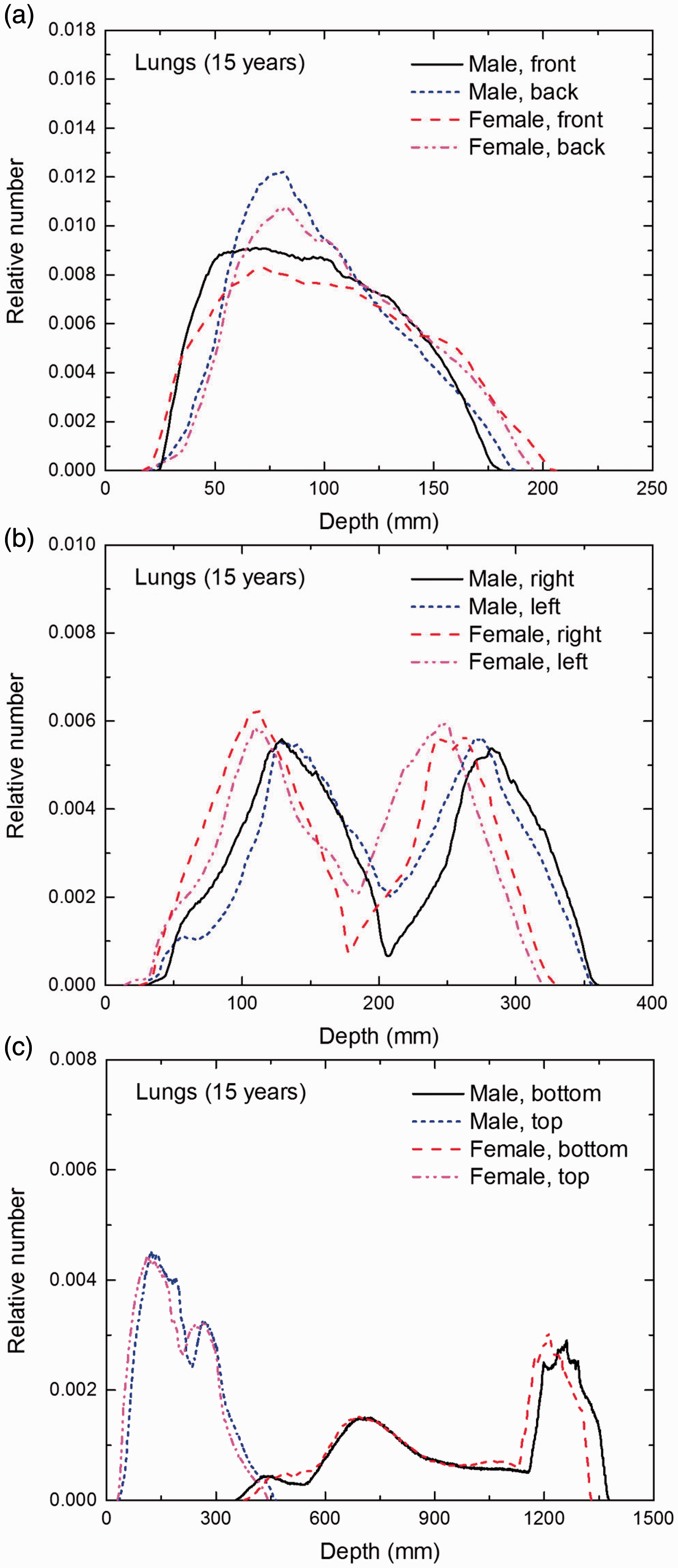
Distribution of depths of 10 million randomly sampled points in the lungs below the body surface of the 15-year-old male/female phantoms at: (a) front and back, (b) right and left, and (c) bottom and top.
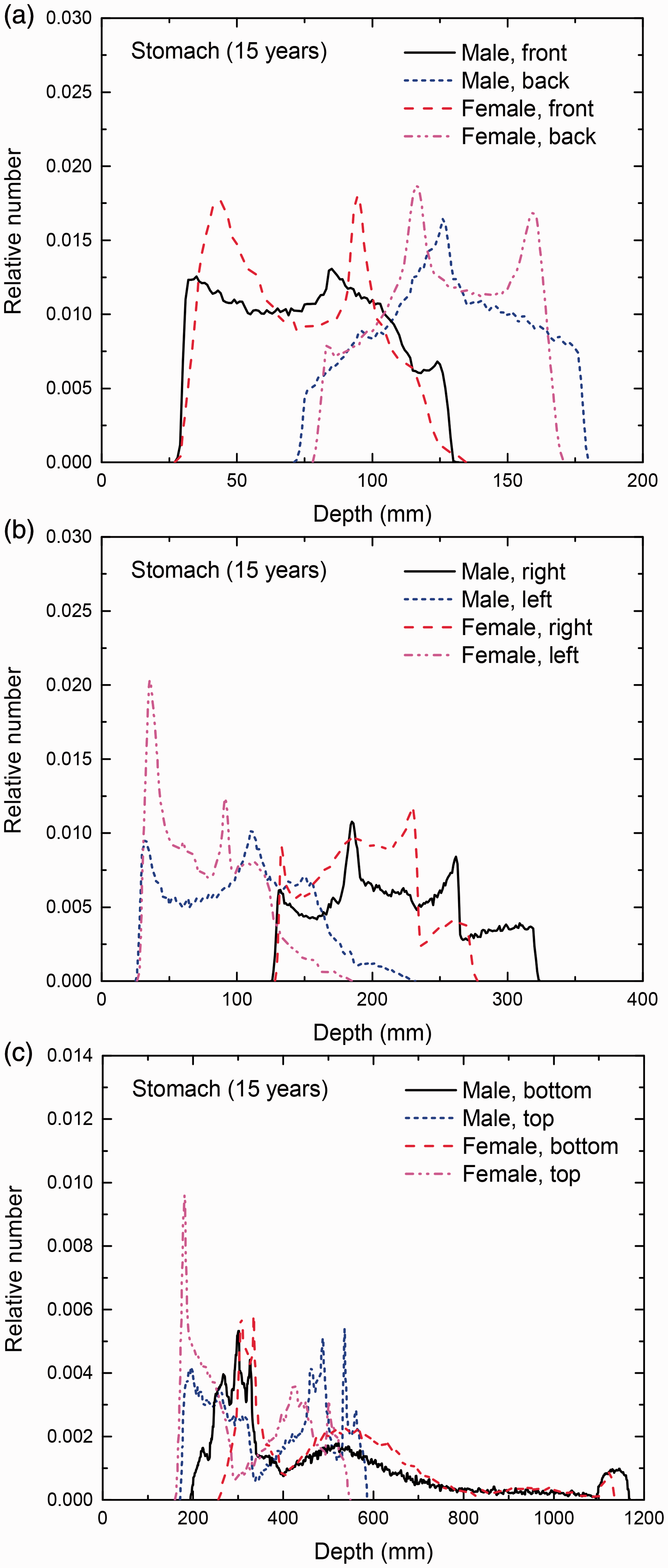
Distribution of depths of 10 million randomly sampled points in the stomach wall below the body surface of the 15-year-old male/female phantoms at: (a) front and back, (b) right and left, and (c) bottom and top.
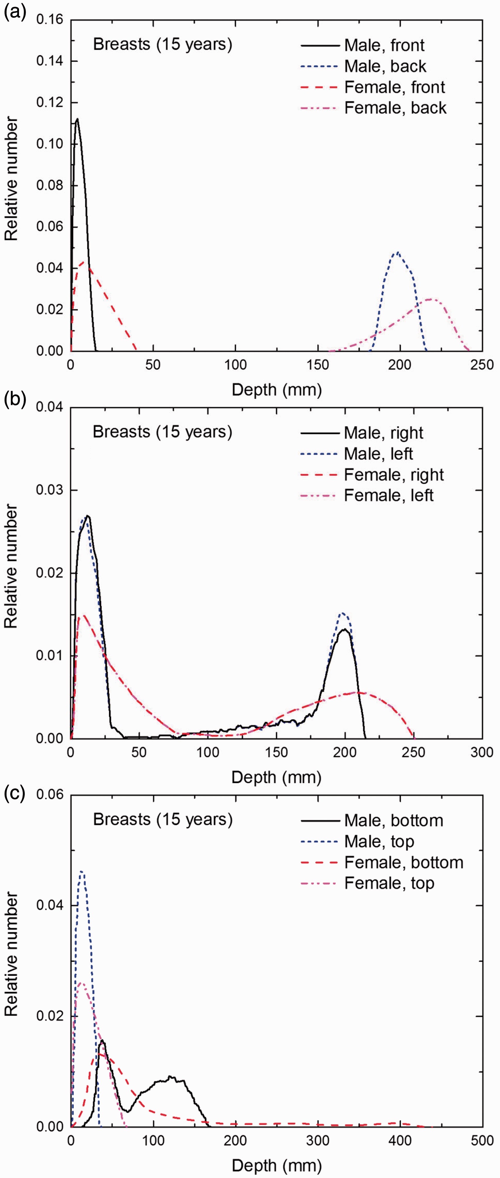
Distribution of depths of 10 million randomly sampled points in the breasts below the body surface of the 15-year-old male/female phantoms at: (a) front and back, (b) right and left, and (c) bottom and top.
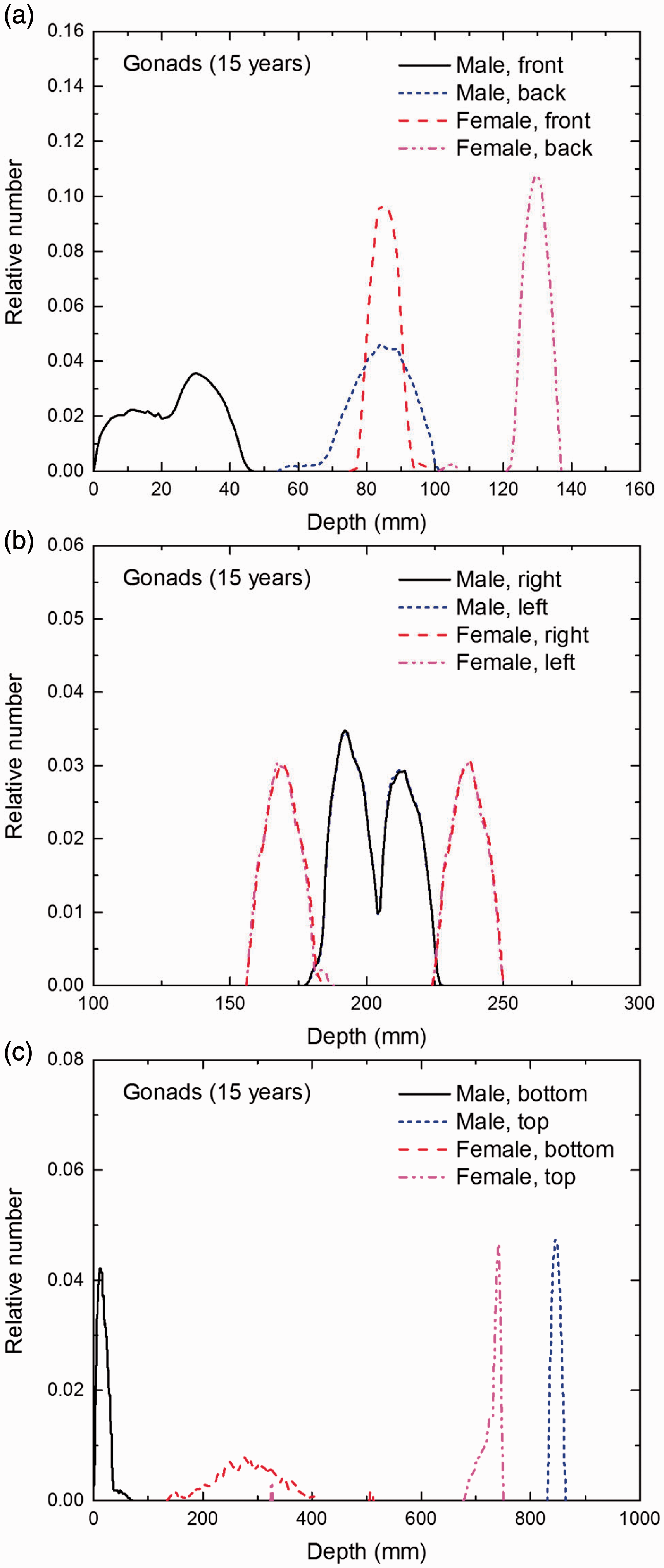
Distribution of depths of 10 million randomly sampled points in the gonads below the body surface of the 15-year-old male/female phantoms at: (a) front and back, (b) right and left, and (c) bottom and top.
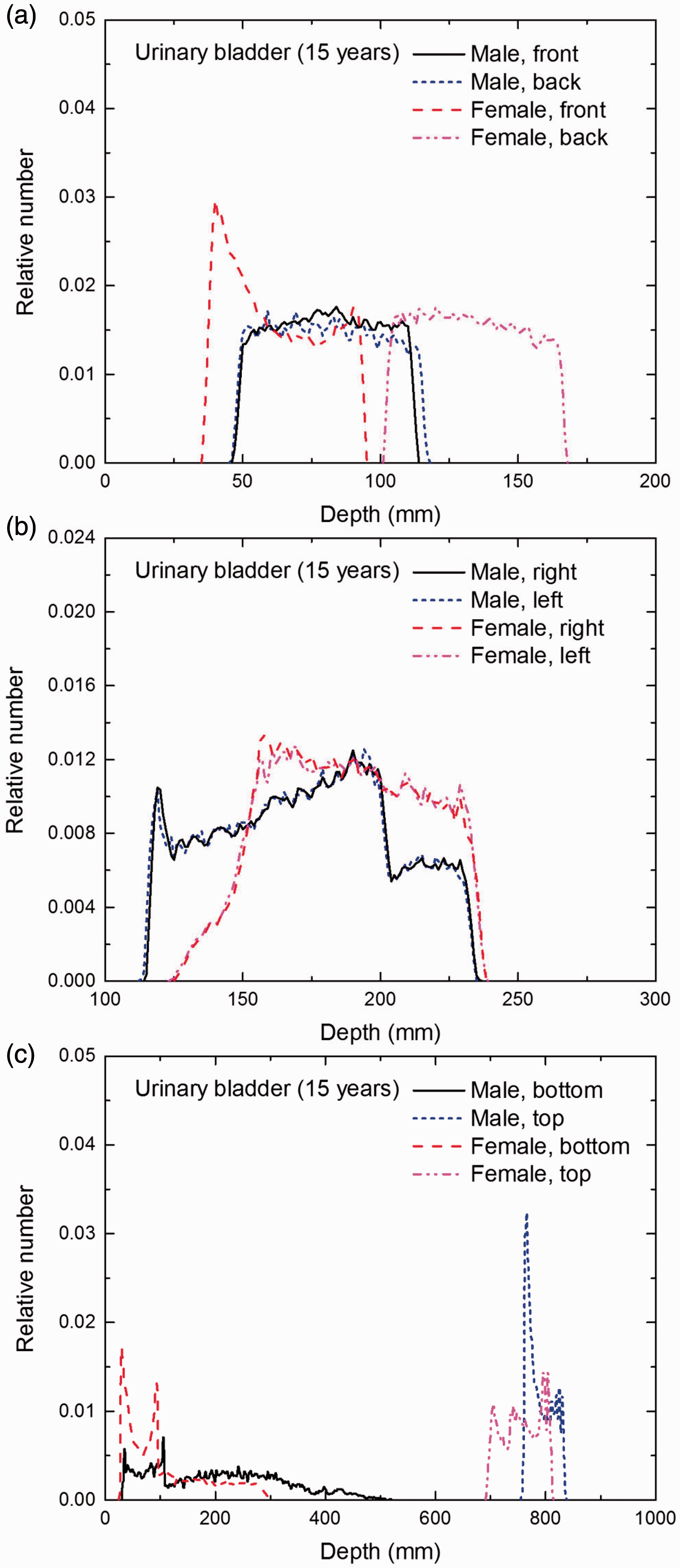
Distribution of depths of 10 million randomly sampled points in the urinary bladder wall below the body surface of the 15-year-old male/female phantoms at: (a) front and back, (b) right and left, and (c) bottom and top.
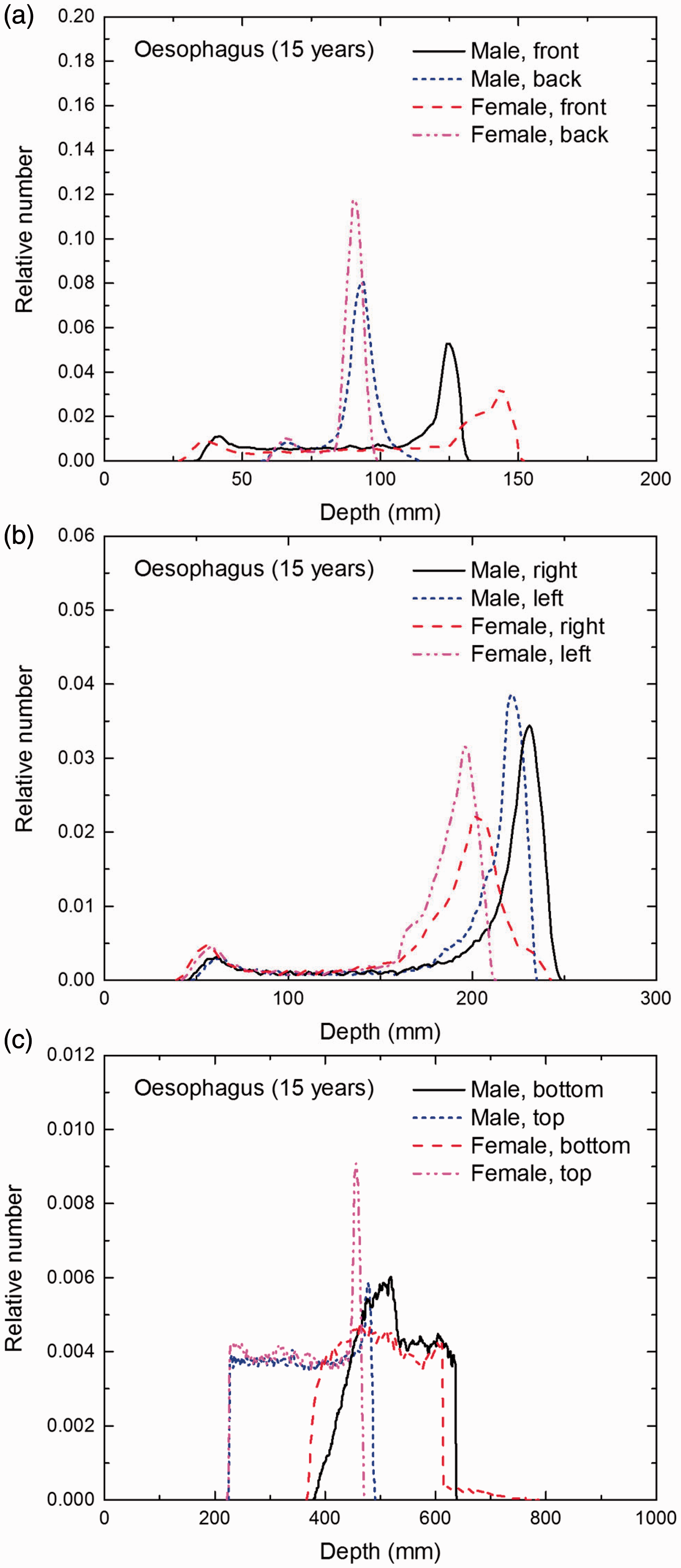
Distribution of depths of 10 million randomly sampled points in the oesophagus wall below the body surface of the 15-year-old male/female phantoms at: (a) front and back, (b) right and left, and (c) bottom and top.
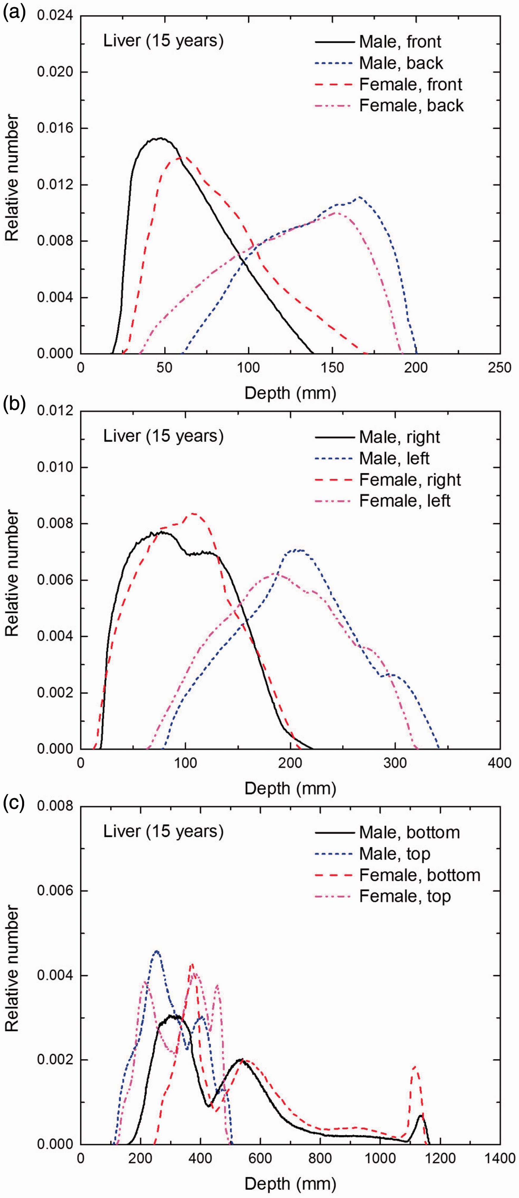
Distribution of depths of 10 million randomly sampled points in the liver below the body surface of the 15-year-old male/female phantoms at: (a) front and back, (b) right and left, and (c) bottom and top.
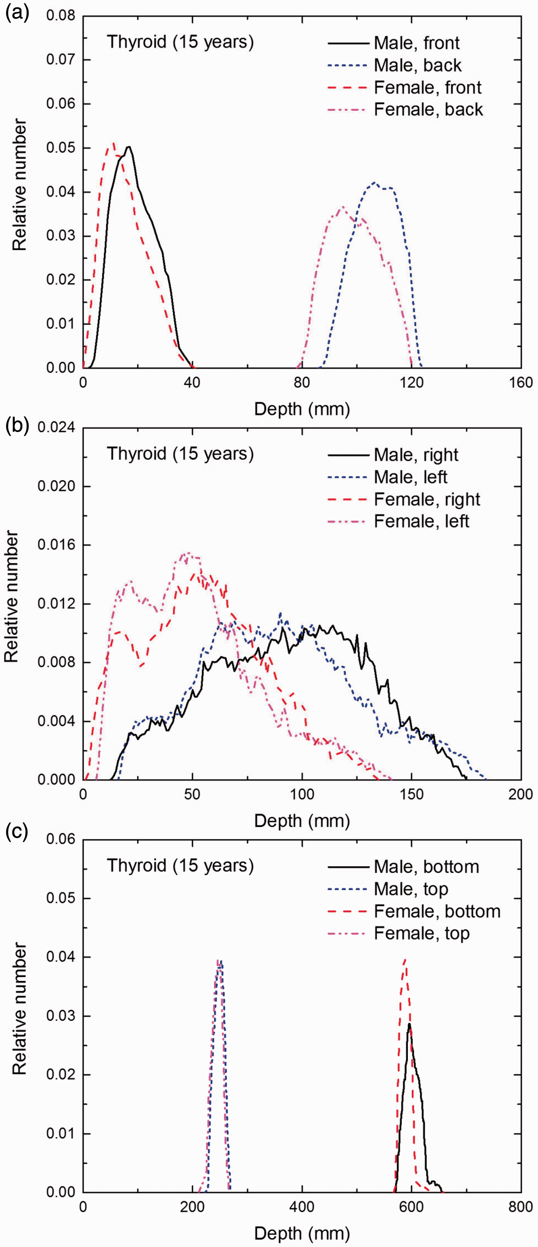
Distribution of depths of 10 million randomly sampled points in the thyroid below the body surface of the 15-year-old male/female phantoms at: (a) front and back, (b) right and left, and (c) bottom and top.
Distribution of depths of 10 million randomly sampled points in the brain below the body surface of the 15-year-old male/female phantoms at: (a) front and back, (b) right and left, and (c) bottom and top.
Distribution of depths of 10 million randomly sampled points in the salivary glands below the body surface of the 15-year-old male/female phantoms at: (a) front and back, (b) right and left, and (c) bottom and top.
Distribution of depths of 10 million randomly sampled points in the skin below the body surface of the 15-year-old male/female phantoms at: (a) front and back, (b) right and left, and (c) bottom and top.
ANNEX F. CHORD-LENGTH DISTRIBUTIONS BETWEEN SELECTED ORGAN PAIRS (SOURCE/TARGET TISSUES)
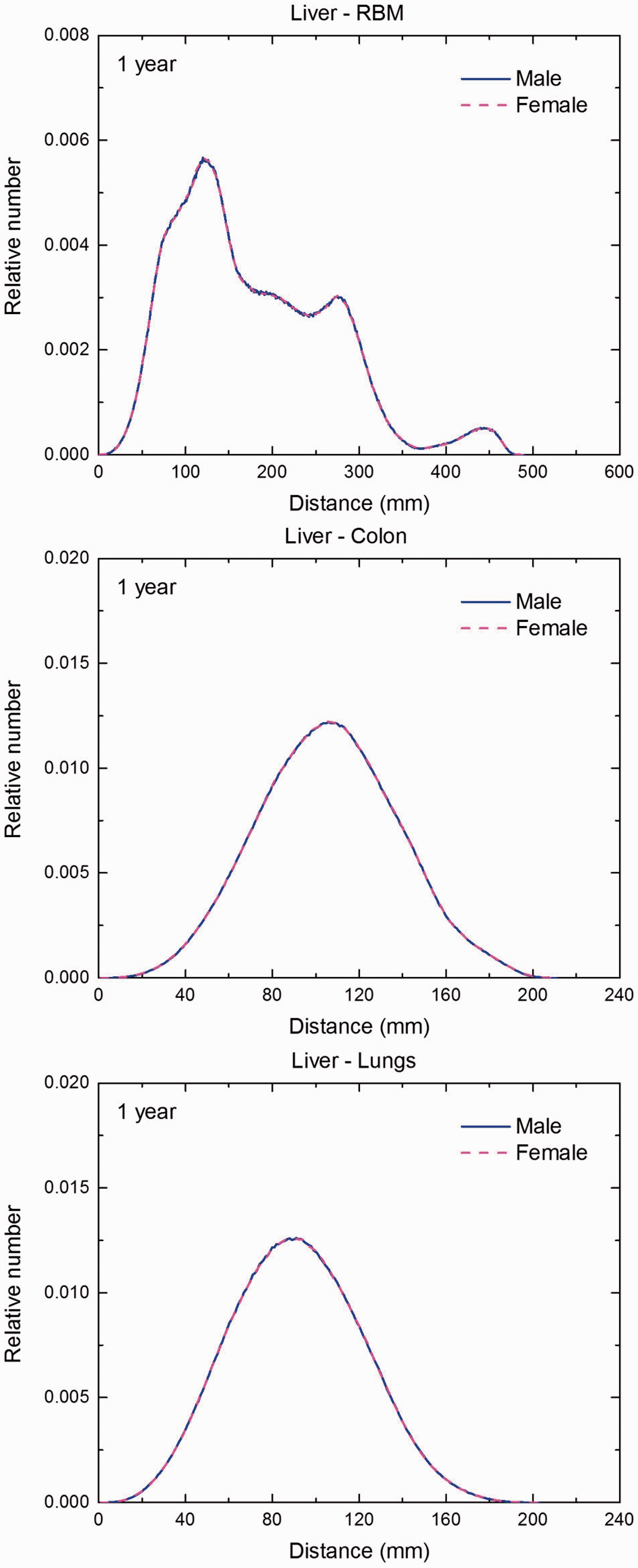
(F1) In Figs F.1–F.20, chord-length distributions are shown between mineral bone, liver, lungs, and thyroid as source organs and the target organs red bone marrow, colon wall, lungs, stomach wall, and breast. Ten million point pairs have been sampled randomly in the organs considered, and the distributions of the resulting chord lengths have been evaluated. (F2) The distance between source and target region is a parameter influencing the SAFs in internal dosimetry.
Distribution of distances between 10 million randomly sampled point pairs in mineral bone (source region) and red bone marrow (RBM), colon, lungs, stomach wall, and breast (target regions) in the newborn male/female phantoms.
Distribution of distances between 10 million randomly sampled point pairs in liver (source region) and red bone marrow (RBM), colon, lungs, stomach wall, and breast (target regions) in the newborn male/female phantoms.
Distribution of distances between 10 million randomly sampled point pairs in lungs (source region) and red bone marrow (RBM), colon, lungs, stomach wall, and breast (target regions) in the newborn male/female phantoms. (continued on next page)
Distribution of distances between 10 million randomly sampled point pairs in thyroid (source region) and red bone marrow (RBM), colon, lungs, stomach wall, and breast (target regions) in the newborn male/female phantoms. (continued on next page)
Distribution of distances between 10 million randomly sampled point pairs in mineral bone (source region) and red bone marrow (RBM), colon, lungs, stomach wall, and breast (target regions) in the 1-year-old male/female phantoms. (continued on next page)
Distribution of distances between 10 million randomly sampled point pairs in liver (source region) and red bone marrow (RBM), colon, lungs, stomach wall, and breast (target regions) in the 1-year-old male/female phantoms. (continued on next page)
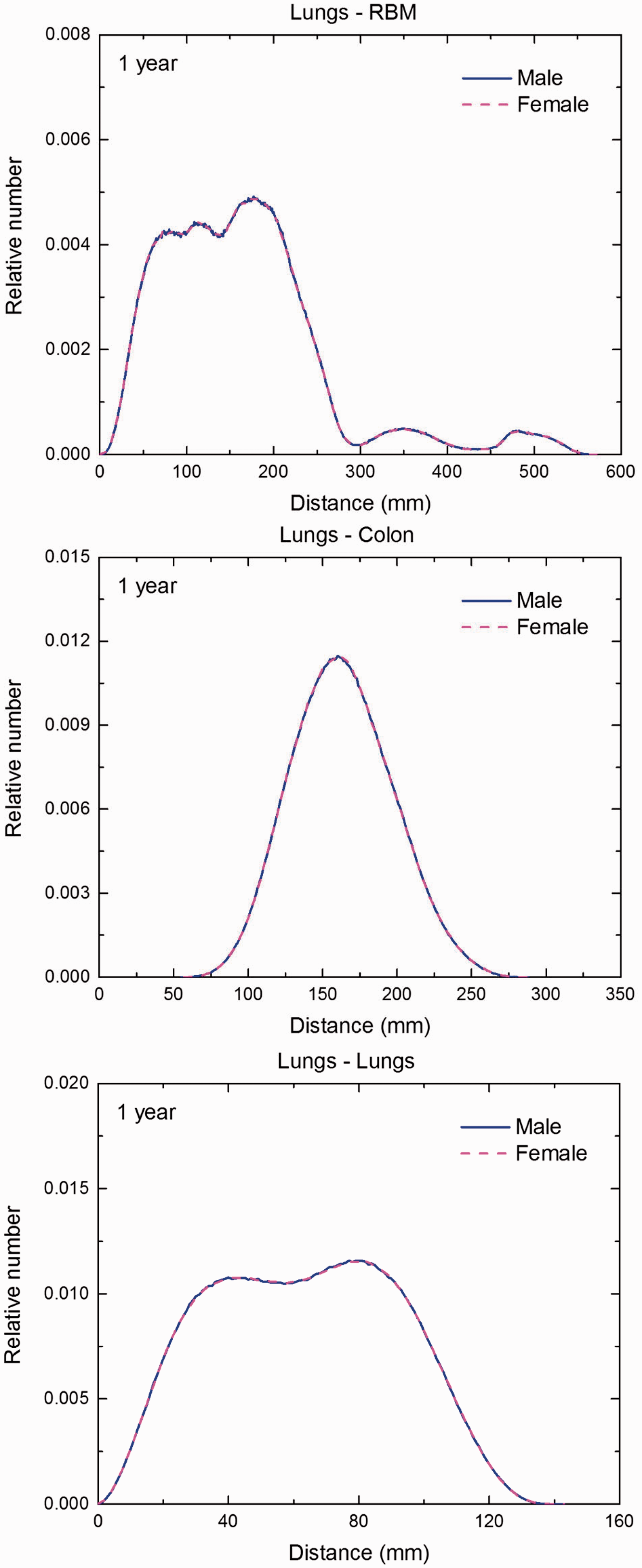
Distribution of distances between 10 million randomly sampled point pairs in lungs (source region) and red bone marrow (RBM), colon, lungs, stomach wall, and breast (target regions) in the 1-year-old male/female phantoms. (continued on next page)
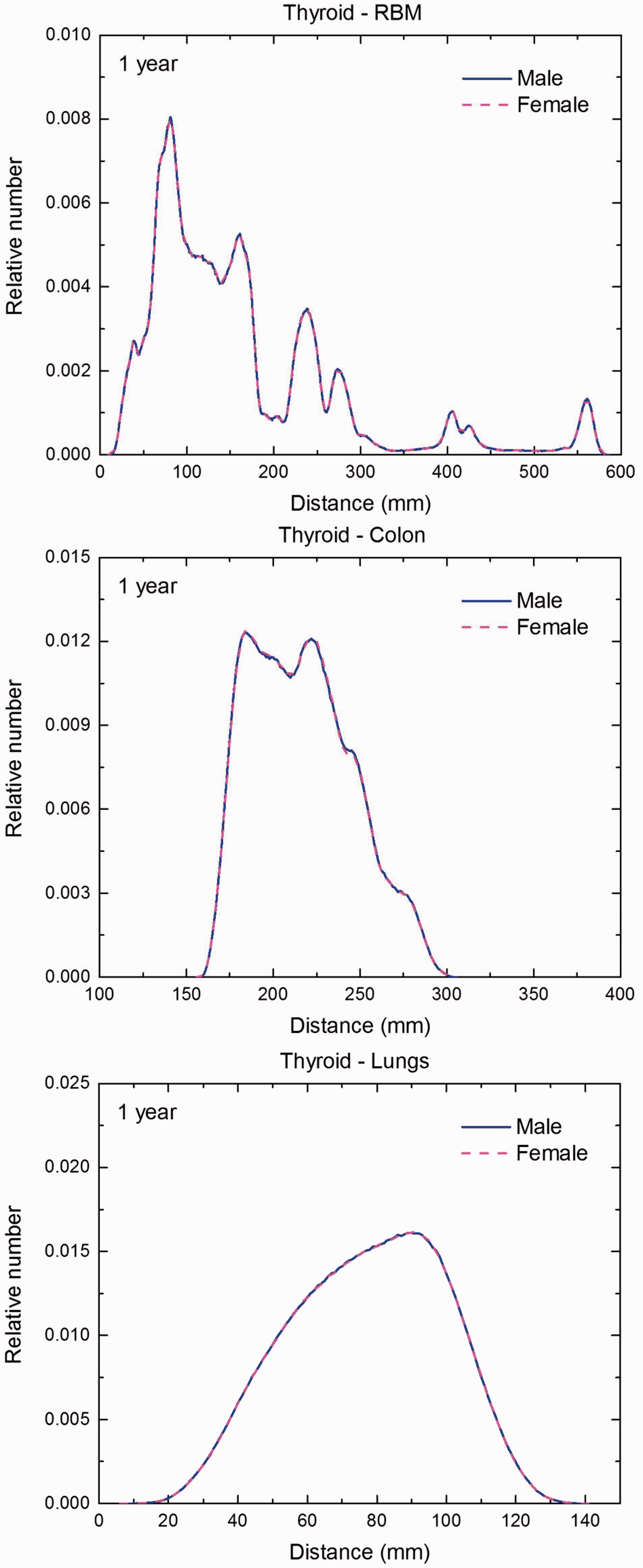
Distribution of distances between 10 million randomly sampled point pairs in thyroid (source region) and red bone marrow (RBM), colon, lungs, stomach wall, and breast (target regions) in the 1-year-old male/female phantoms. (continued on next page)
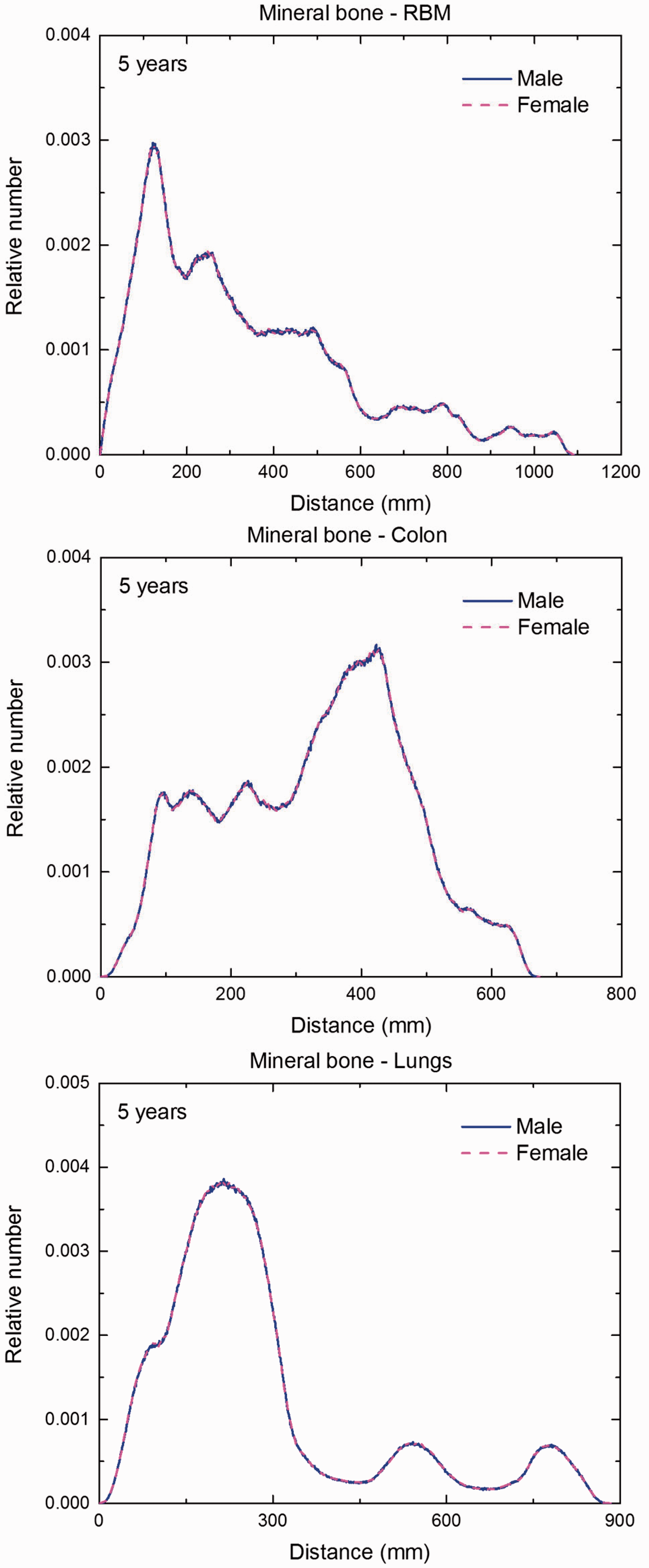
Distribution of distances between 10 million randomly sampled point pairs in mineral bone (source region) and red bone marrow (RBM), colon, lungs, stomach wall, and breast (target regions) in the 5-year-old male/female phantoms. (continued on next page)
Distribution of distances between 10 million randomly sampled point pairs in liver (source region) and red bone marrow (RBM), colon, lungs, stomach wall, and breast (target regions) in the 5-year-old male/female phantoms. (continued on next page)
Distribution of distances between 10 million randomly sampled point pairs in lungs (source region) and red bone marrow (RBM), colon, lungs, stomach wall, and breast (target regions) in the 5-year-old male/female phantoms. (continued on next page)
Distribution of distances between 10 million randomly sampled point pairs in thyroid (source region) and red bone marrow (RBM), colon, lungs, stomach wall, and breast (target regions) in the 5-year-old male/female phantoms. (continued on next page)
Distribution of distances between 10 million randomly sampled point pairs in mineral bone (source region) and red bone marrow (RBM), colon, lungs, stomach wall, and breast (target regions) in the 10-year-old male/female phantoms. (continued on next page)
Distribution of distances between 10 million randomly sampled point pairs in liver (source region) and red bone marrow (RBM), colon, lungs, stomach wall, and breast (target regions) in the 10-year-old male/female phantoms. (continued on next page)
Distribution of distances between 10 million randomly sampled point pairs in lungs (source region) and red bone marrow (RBM), colon, lungs, stomach wall, and breast (target regions) in the 10-year-old male/female phantoms. (continued on next page)

Distribution of distances between 10 million randomly sampled point pairs in thyroid (source region) and red bone marrow (RBM), colon, lungs, stomach wall, and breast (target regions) in the 10-year-old male/female phantoms. (continued on next page)
Distribution of distances between 10 million randomly sampled point pairs in mineral bone (source region) and red bone marrow (RBM), colon, lungs, stomach wall, and breast (target regions) in the 15-year-old male/female phantoms. (continued on next page)
Distribution of distances between 10 million randomly sampled point pairs in liver (source region) and red bone marrow (RBM), colon, lungs, stomach wall, and breast (target regions) in the 15-year-old male/female phantoms. (continued on next page)
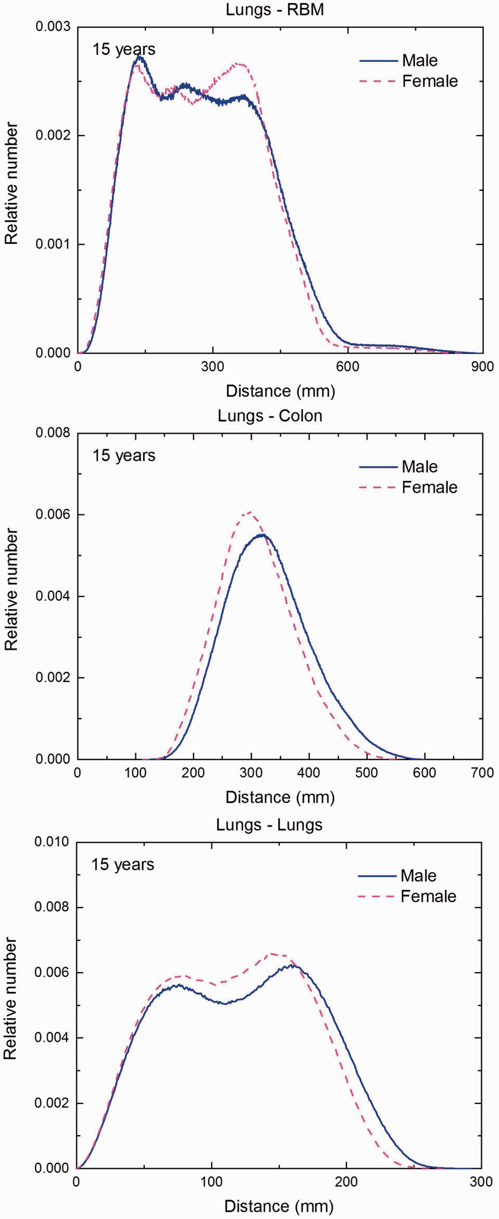
Distribution of distances between 10 million randomly sampled point pairs in lungs (source region) and red bone marrow (RBM), colon, lungs, stomach wall, and breast (target regions) in the 15-year-old male/female phantoms. (continued on next page)
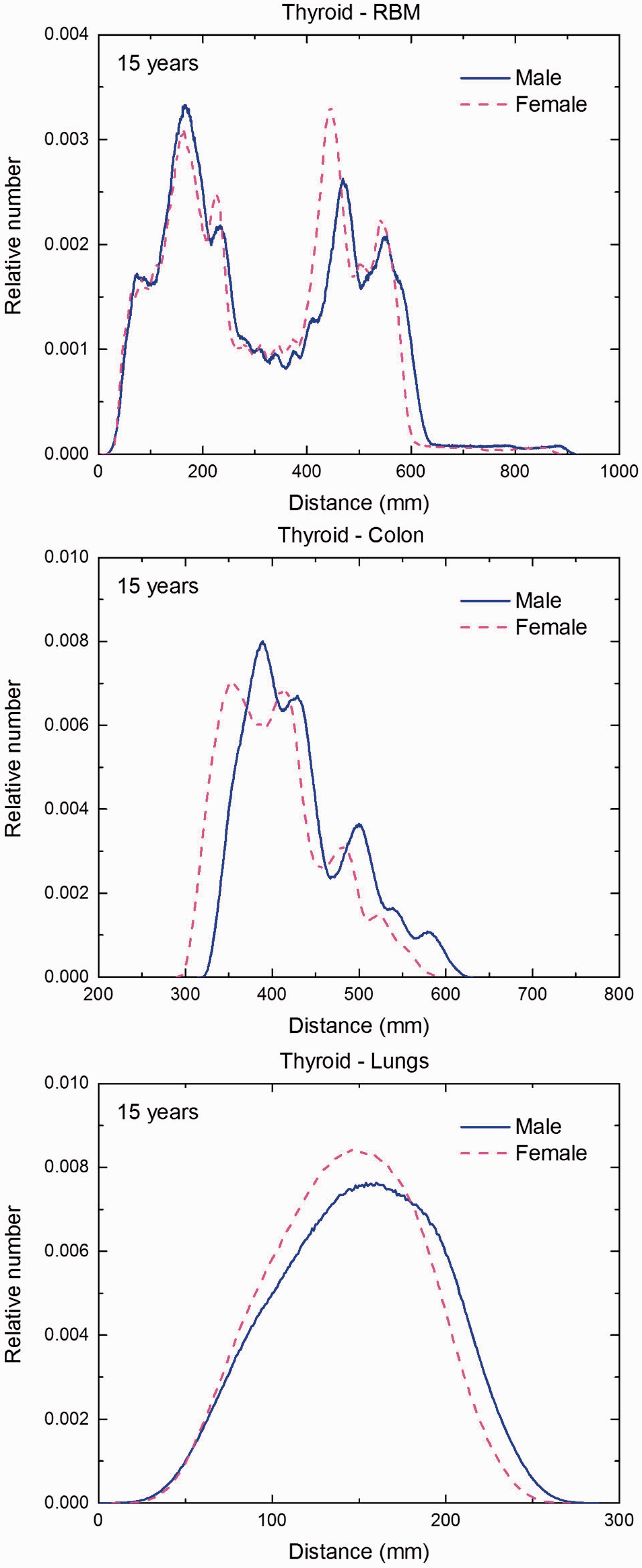
Distribution of distances between 10 million randomly sampled point pairs in thyroid (source region) and red bone marrow (RBM), colon, lungs, stomach wall, and breast (target regions) in the 15-year-old male/female phantoms. (continued on next page)
ANNEX G. CROSS-SECTIONAL VIEWS FOR SELECTED PHANTOMS AND BODY REGIONS
(G1) This annex presents selected cross-sectional images of the paediatric reference computational phantoms. The cross-sectional images are presented in three different orientations: transverse, coronal, and sagittal. Each cross-sectional image presents a planar ‘cut’ through the three-dimensional voxel array describing the computational phantom. The transverse images show the columns (x coordinates) and rows (y coordinates) at a specific slice (z coordinate); the coronal images show the columns and slices at a specific row; and the sagittal images show the rows and slices at a specific column. (G2) The green lines indicate the location of single organs as given in the legend. The yellow lines (appearing as a coordinate cross in the figures) indicate the location of the images in the other orientations. In the transverse images, the vertical yellow line indicates the location of the sagittal image, and the horizontal yellow line indicates the location of the coronal image.
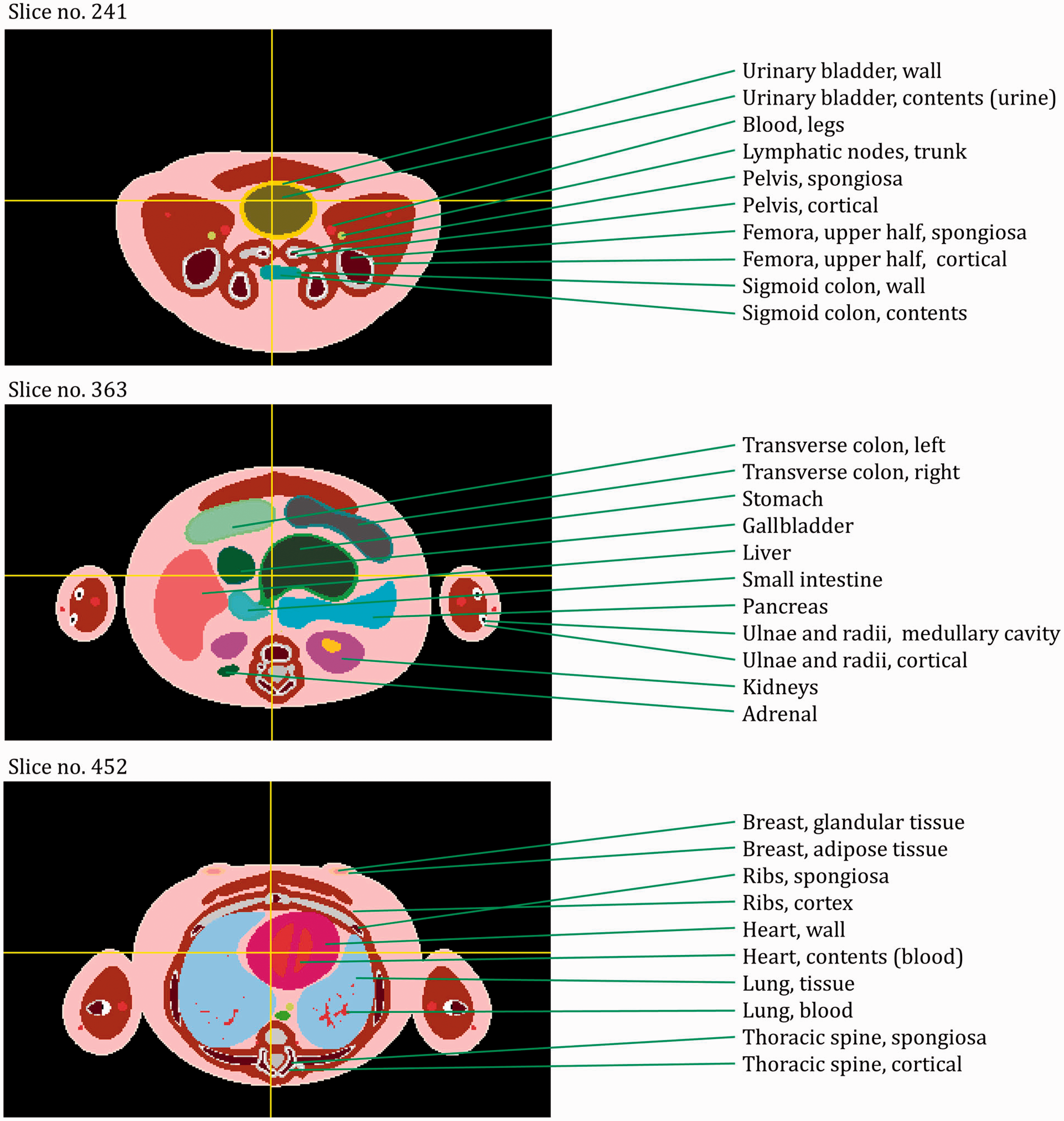
Transverse (axial) images of the newborn male phantom. ET, extrathoracic. (continued on next page)
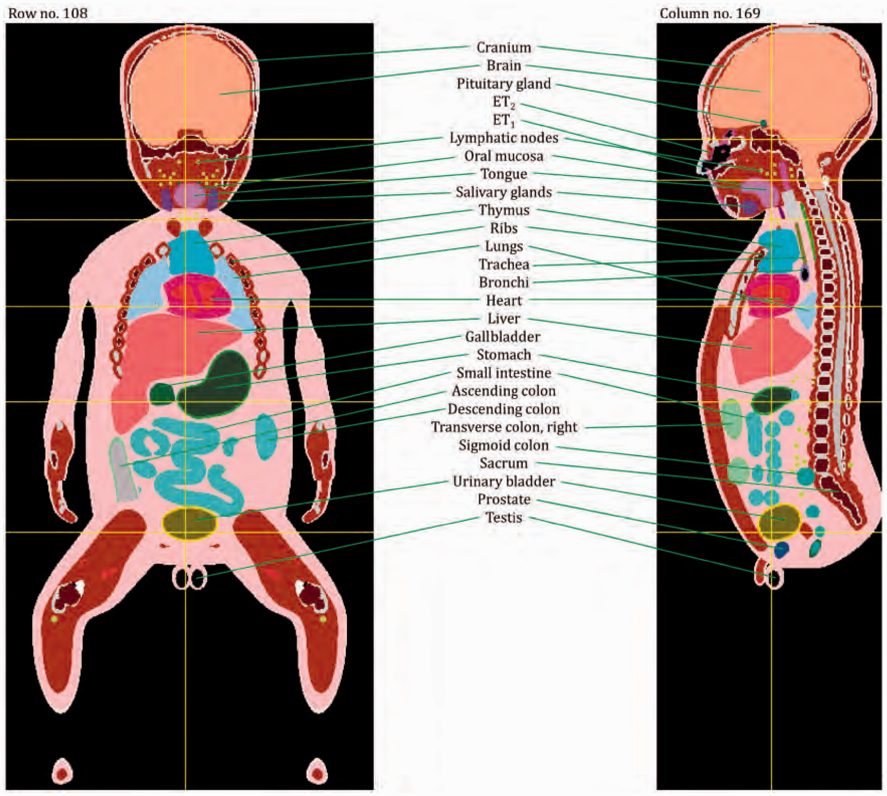
Coronal and sagittal images of the newborn male phantom. ET, extrathoracic.
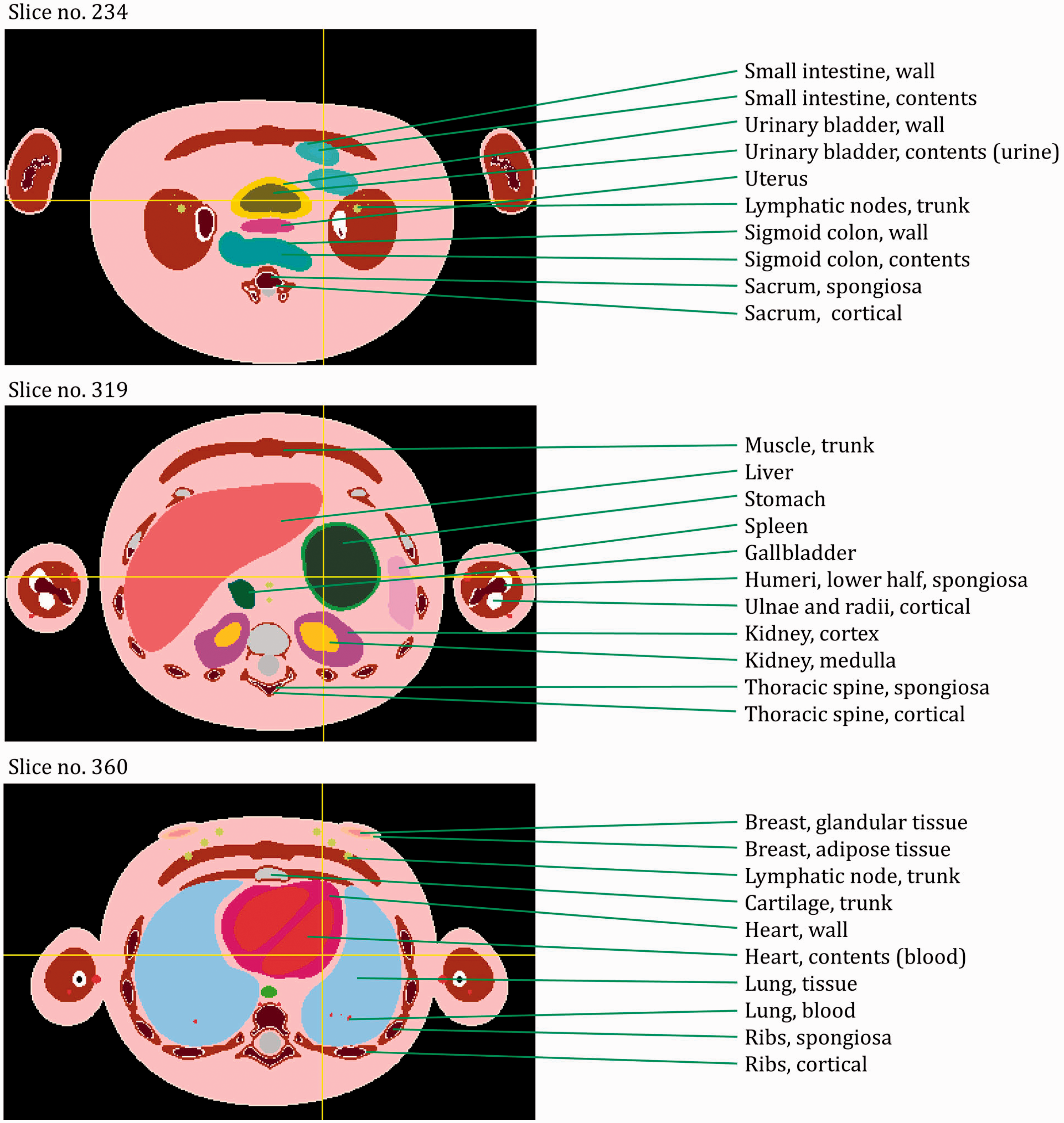
Transverse (axial) images of the 1-year-old female phantom. ET, extrathoracic. (continued on next page)
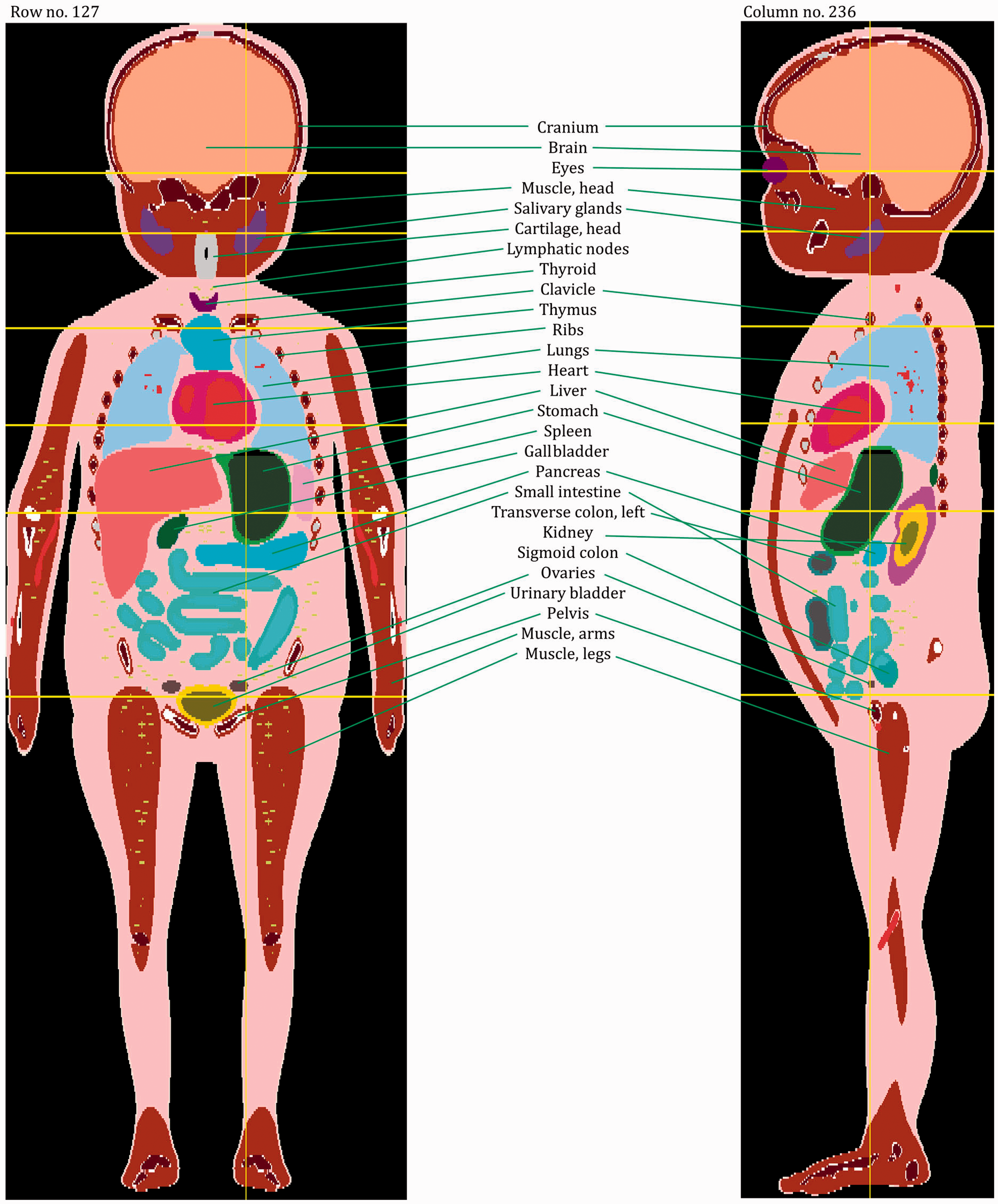
Coronal and sagittal images of the 1-year-old female phantom.
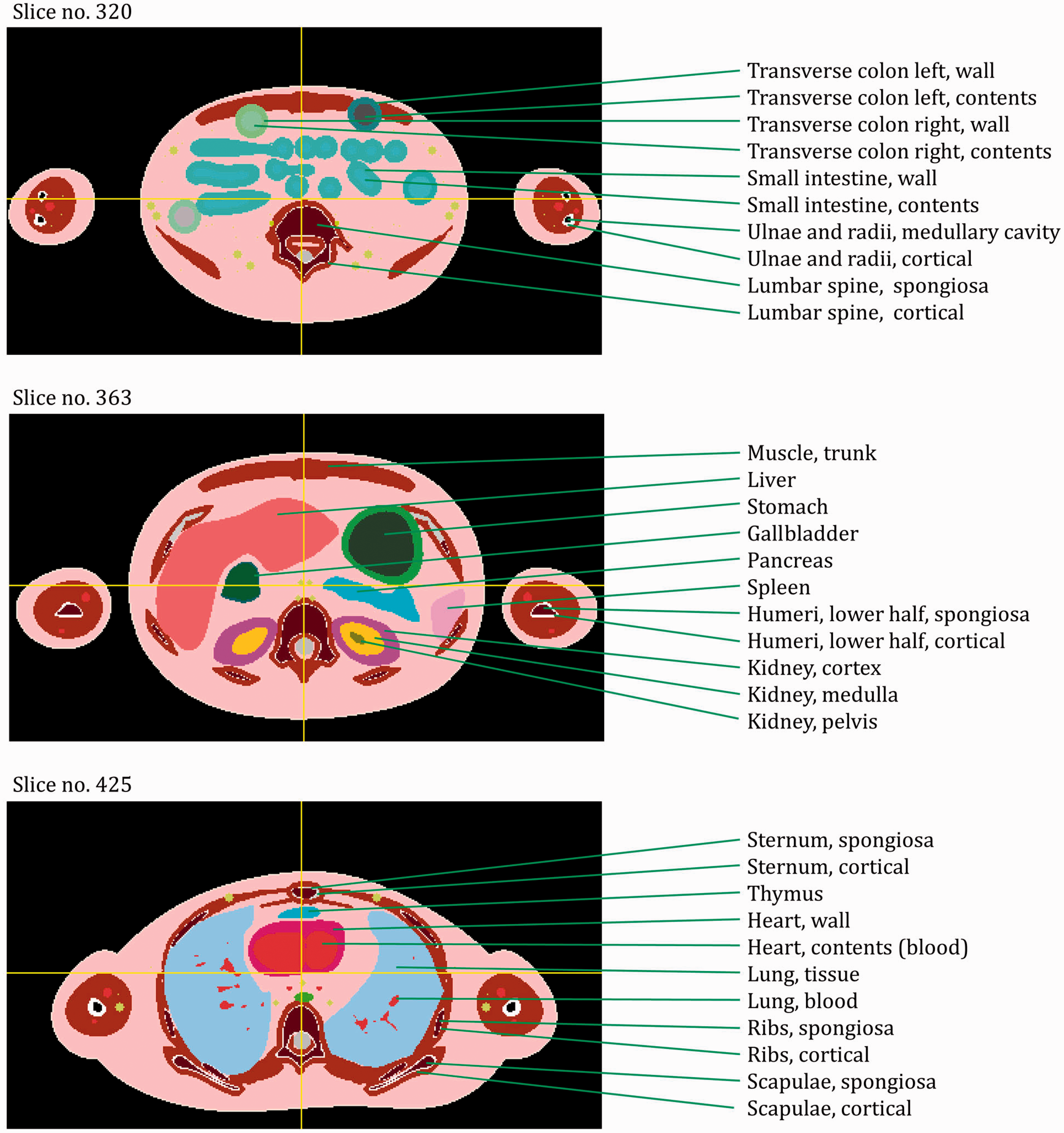
Transverse (axial) images of the 5-year-old male phantom. ET, extrathoracic. (continued on next page)
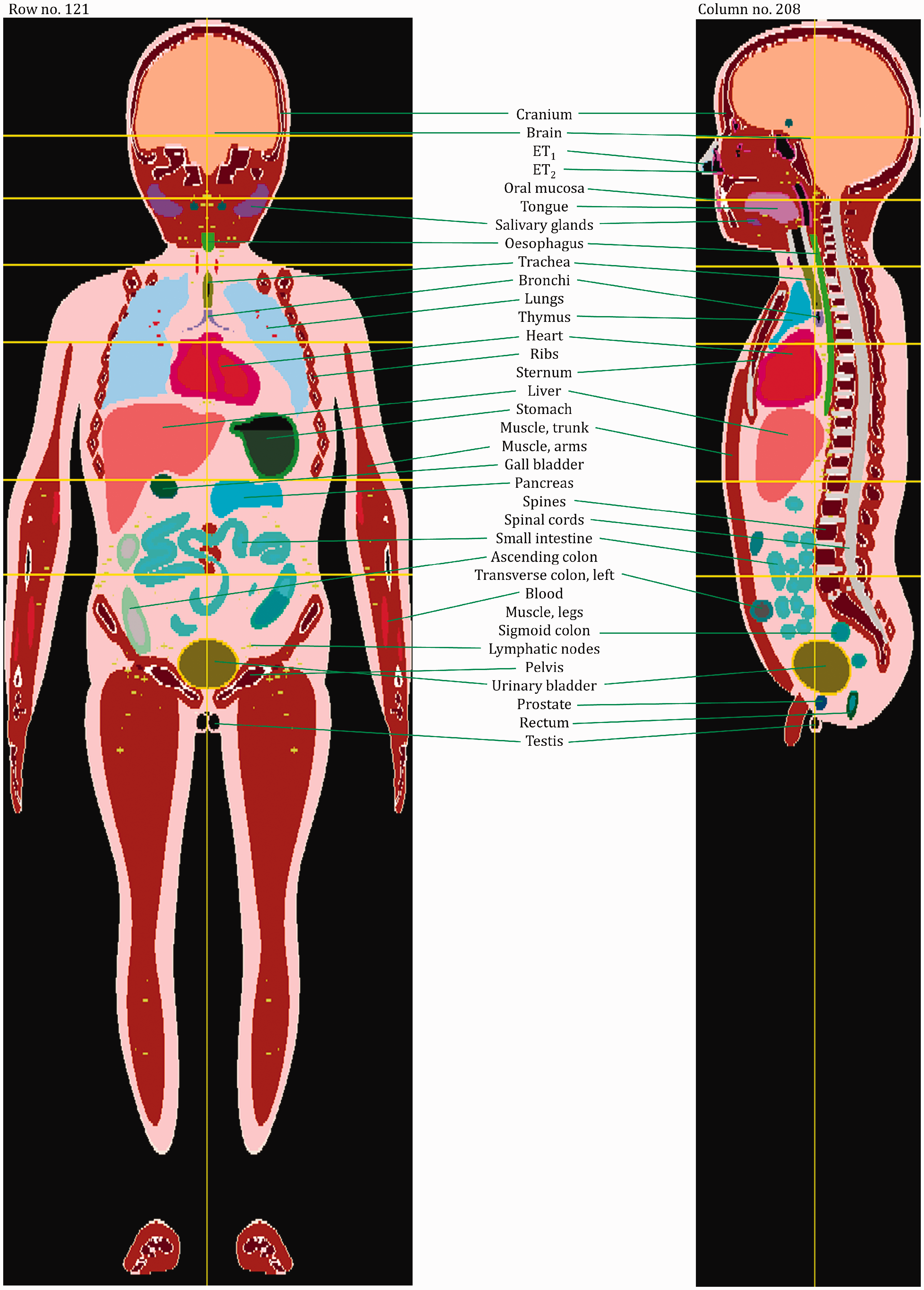
Coronal and sagittal images of the 5-year-old male phantom. ET, extrathoracic.
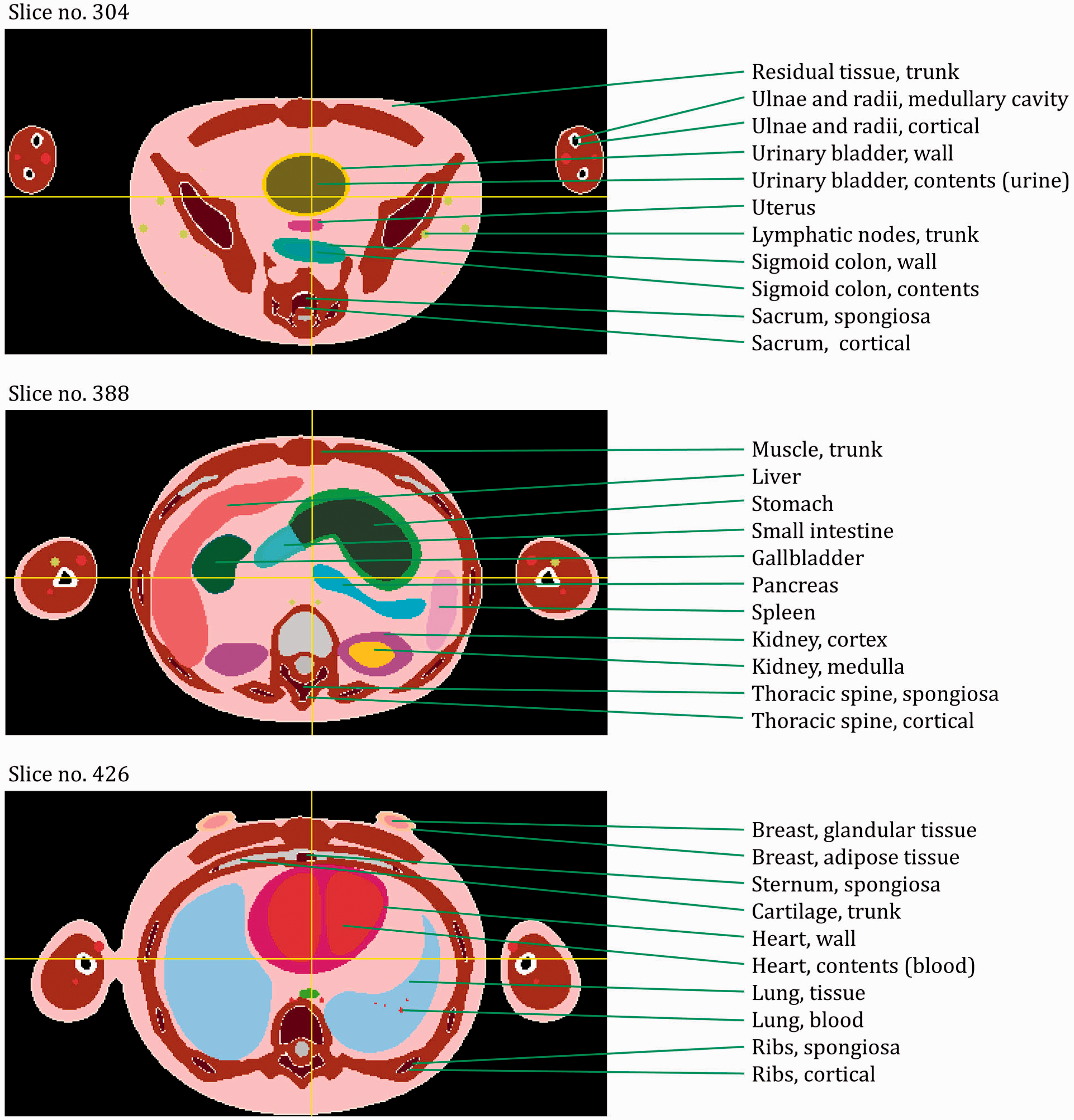
Transverse (axial) images of the 10-year-old female phantom. ET, extrathoracic. (continued on next page)
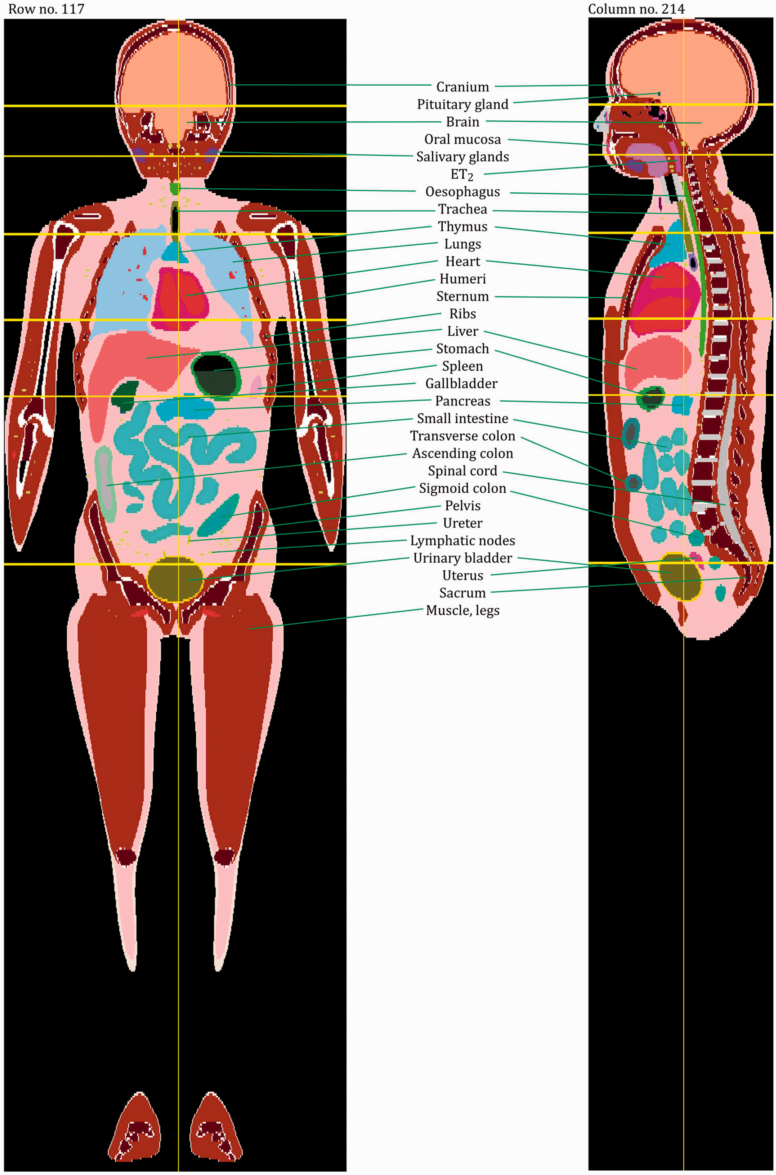
Coronal and sagittal images of the 10-year-old female phantom. ET, extrathoracic.
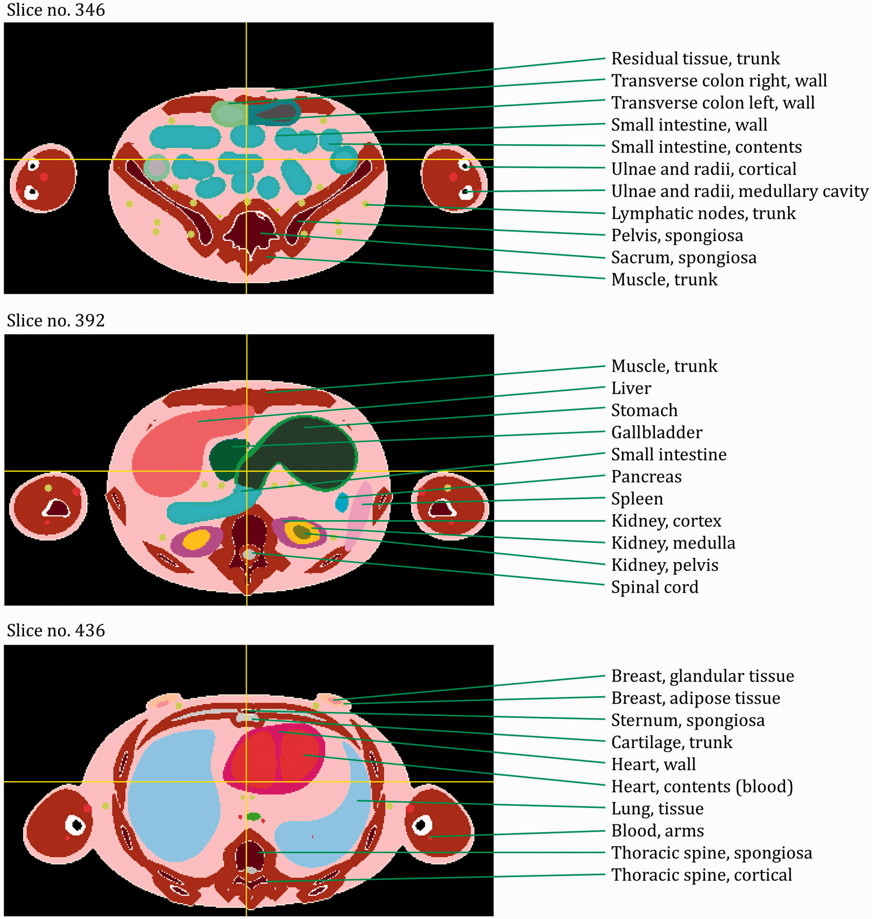
Transverse (axial) images of the 15-year-old male phantom. ET, extrathoracic. (continued on next page)
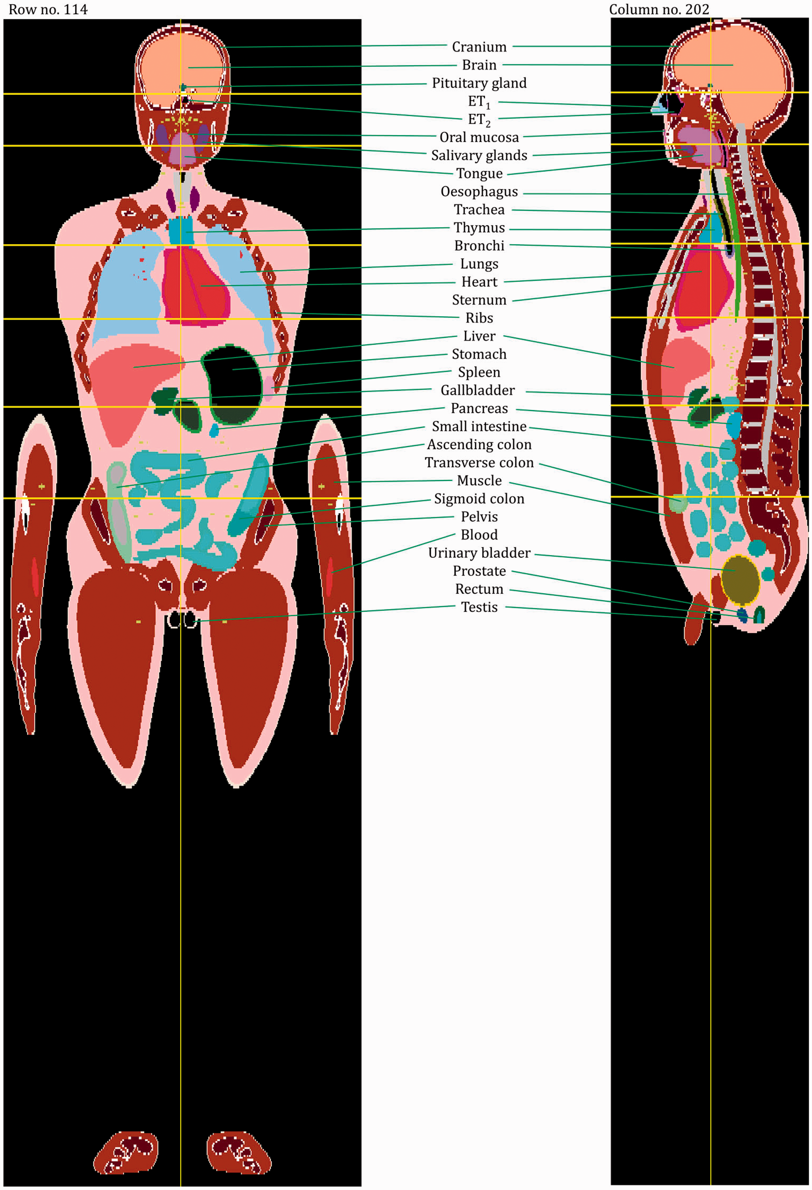
Coronal and sagittal images of the 15-year-old male phantom. ET, extrathoracic.
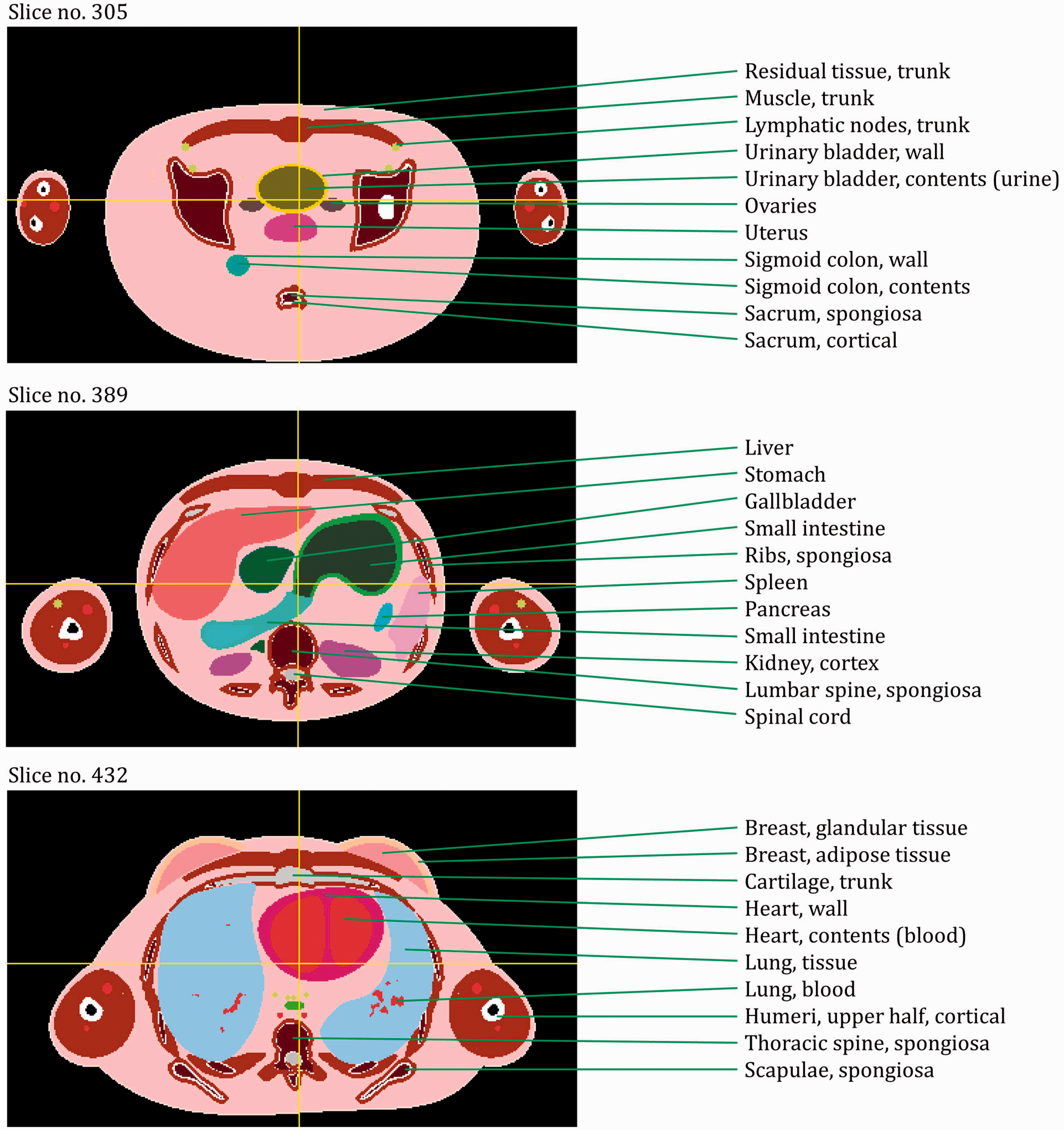
Transverse (axial) images of the 15-year-old female phantom. ET, extrathoracic. (continued on next page)
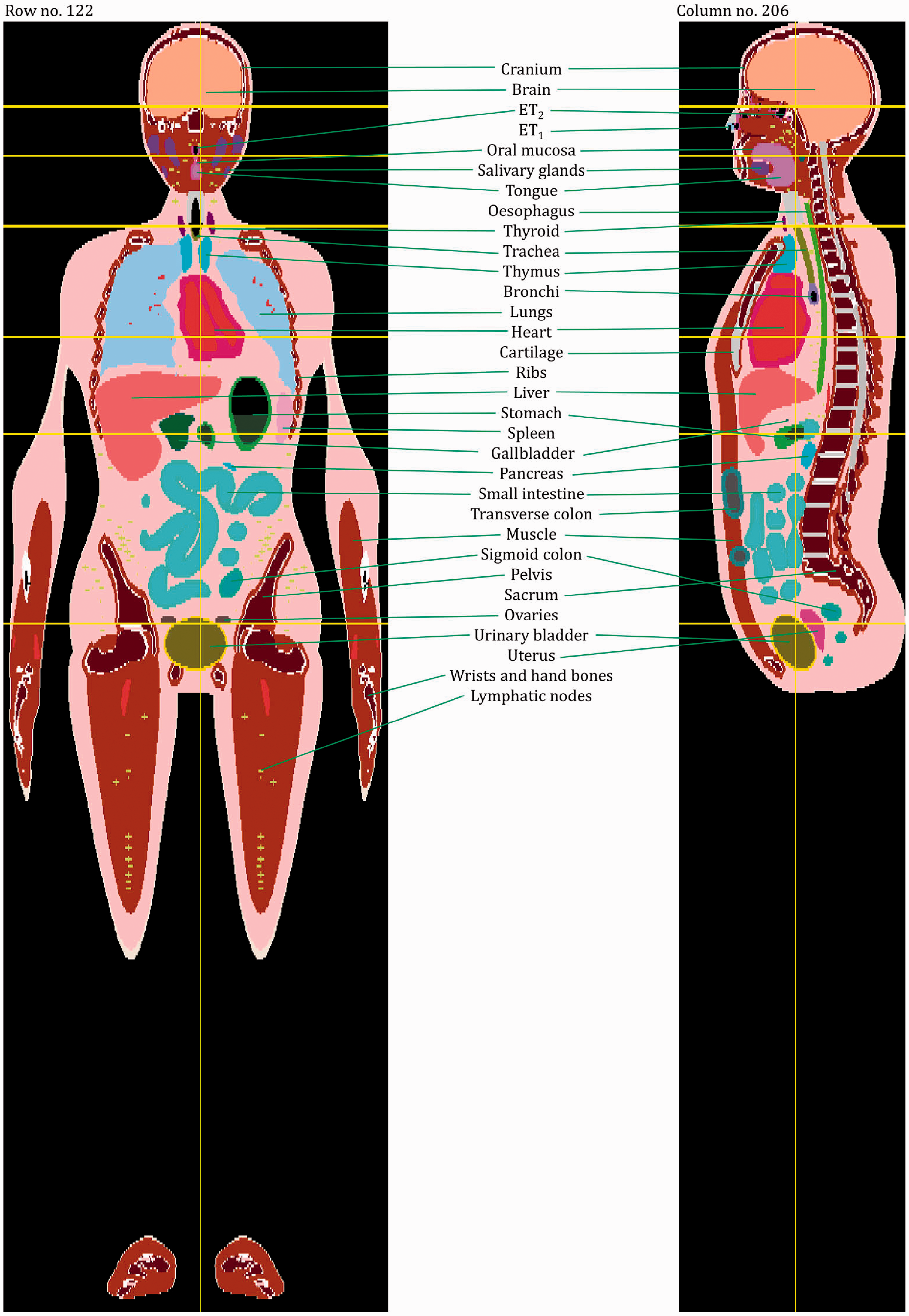
Coronal and sagittal images of the 15-year-old female phantom. ET, extrathoracic.
ANNEX H. DESCRIPTION OF THE ELECTRONIC FILES FOR THE PAEDIATRIC PHANTOMS
(H1) The data files for the paediatric reference phantoms are available for download from www.icrp.org. The data files are organised into 10 main folders, one for each of the 10 reference phantoms (00 M, newborn male; 00 F, newborn female; 01 M, 1-year-old male; 01 F, 1-year-old female; 05 M, 5-year-old male; 05 F, 5-year-old female; 10 M, 10-year-old male; 10 F, 10-year-old female; 15 M, 15-year-old male; 15 F, 15-year-old female). Each folder contains the following files:
The array of organ ID numbers in ASCII format and binary format; the file names are:
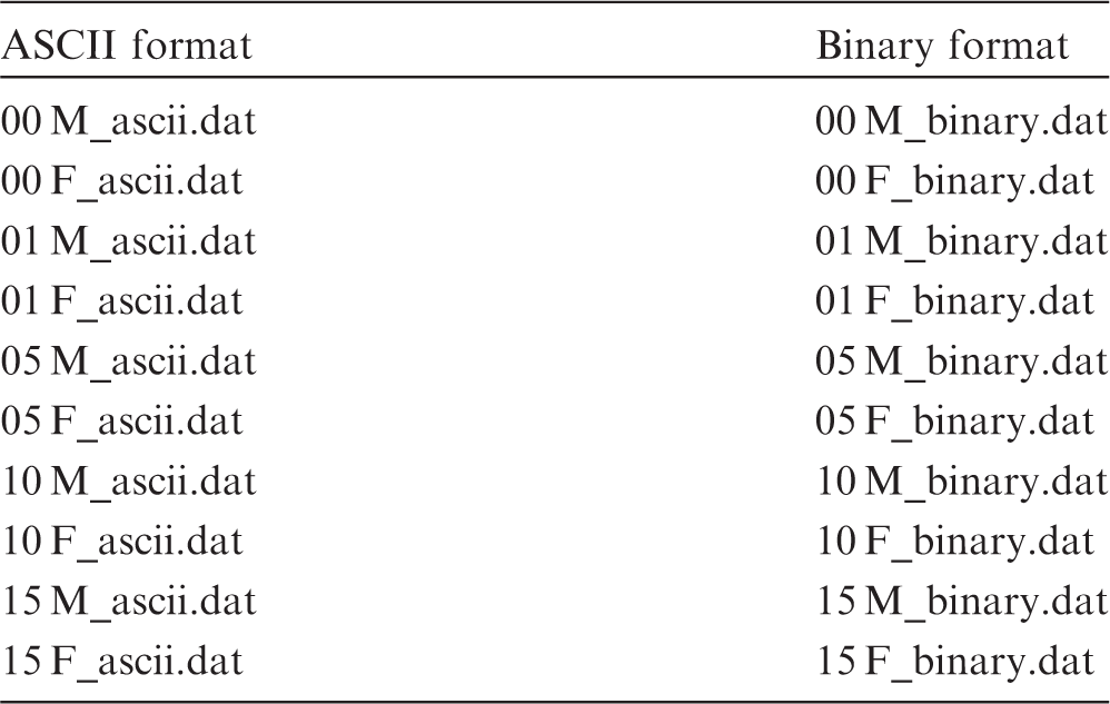
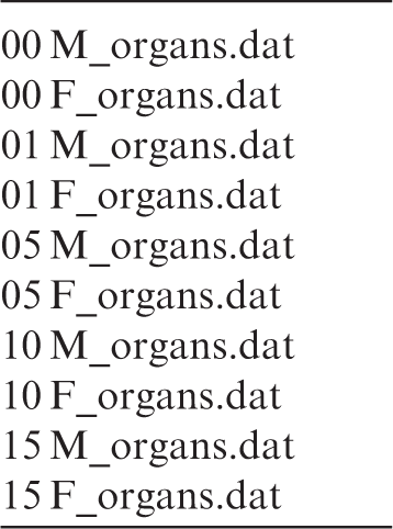
A list of individually segmented structures, their ID numbers, and assigned media (Annex A); the file names are:
A list of the media, their elemental compositions, and densities (Annex B); the file names are:
A list of the skeletal tissue masses and surface areas in skeletal sites (Tables 3.3–3.8); the file names are:
A list of regional blood distributions (Table 4.3); the file names are:
(H2) In the organ ID arrays, the organ IDs are listed slice by slice; within each slice, row by row; and within each row, column by column. That means, the column index changes most quickly, then the row index, then the slice index. The numbers of columns, rows, and slices (i.e. the array dimensions) of the phantoms are given in Table 4.1, together with the voxel resolutions.
GLOSSARY
Absorbed dose, D The absorbed dose is given by:
Active marrow is haematopoietically active and gets its red colour from the large numbers of erythrocytes (red blood cells) being produced. Active bone marrow serves as a target region for radiogenic risk of leukaemia. See also ‘Active (bone) marrow’; ‘Inactive (bone) marrow’. Bone marrow is a soft, highly cellular tissue that occupies the cylindrical cavities of long bones and the cavities defined by the bone trabeculae of the axial and appendicular skeleton. Total bone marrow consists of a sponge-like, reticular, connective tissue framework called ‘stroma’, myeloid (blood-cell-forming) tissue, fat cells (adipocytes), small accumulations of lymphatic tissue, and numerous blood vessels and sinusoids. There are two types of bone marrow – active (red) and inactive (yellow) – where these adjectives refer to the marrow’s potential for blood cell element production (haematopoiesis). The marrow contained in the medullary cavities in the shafts of the long bones. In accordance with the generic definition of effective dose in Publication 103 (ICRP, 2007), the effective dose is calculated as:
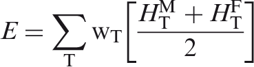
Endosteum (or endosteal layer) A 50-µm-thick layer covering the surfaces of the bone trabeculae in regions of trabecular spongiosa and those of the cortical surfaces of the medullary cavities within the shafts of all long bones. It is assumed to be the target region for radiogenic bone cancer. This target region replaces that previously introduced in Publications 26 and 30 – the bone surfaces – which had been defined as a single-cell layer, 10 µm in thickness, covering the surfaces of both the bone trabeculae and the Haversian canals of cortical bone.
Equivalent dose, HT The equivalent dose to a tissue or organ is defined as:
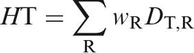
Identification (ID) number Number assigned unequivocally to each individually segmented organ/tissue.
Inactive (bone) marrow In contrast to the active marrow, the inactive marrow is haematopoietically inactive (i.e. does not support haematopoiesis directly). It gets its yellow colour from fat cells (adipocytes) which occupy most of the space in the bone marrow framework.
Marrow cellularity The fraction of bone marrow volume in a given bone that is haematopoietically active. Age- and bone-site-dependent reference values for marrow cellularity are given in Table 41 of Publication 70 (ICRP, 1995). As a first approximation, marrow cellularity may be thought of as 1 minus the fat fraction of bone marrow. See ‘Active (bone) marrow’. An idealised male or female with anatomical and physiological characteristics defined by ICRP for the purpose of radiological protection. Reference Individuals are defined in Publication 89 (ICRP, 2002) for male and female newborn, 1-year-old, 5-year-old, 10-year-old, 15-year-old, and adult. Consequently, there are 12 Reference Individuals within the ICRP system of radiation protection. An idealised person for whom the equivalent doses to organs and tissues are calculated by averaging the corresponding doses of Reference Male and Female. The equivalent doses of the Reference Person are used for calculation of the effective dose. There are thus six Reference Persons within the ICRP system of radiological protection, one at each of the reference ages defined in Publication 89 (ICRP, 2002). The value of a parameter, factor, or quantity that is regarded as valid for use in dosimetric calculations and recommended by ICRP. These values are fixed and are not subject to uncertainties. A function representing the absorbed dose in a target region per particle fluence in the region, derived using models of the microscopic structure of the target region geometry, and the transport of the secondary ionising radiations in those regions. Region of the body containing the radionuclide. The region may be an organ, a tissue, the contents of the alimentary tract or urinary bladder, or the surfaces of tissues as in the skeleton and the respiratory tract. Term referring to the combined tissues of the bone trabeculae and marrow tissues (both active and inactive) located beneath the cortical bone cortices across regions of the axial and appendicular skeleton. Spongiosa is one of three bone regions defined in Publication 110 (ICRP, 2009) reference phantoms, the other two being cortical bone and medullary marrow of the long bone shafts. As the relative proportions of trabecular bone, active marrow, and inactive marrow vary with skeletal site and reference phantom age, the homogeneous elemental composition and mass density of spongiosa are not constant, but vary with skeletal site and phantom age. Organ or tissue region of the body in which a radiation absorbed dose is received. Organs or tissues in the body for which radiation weighting factors are assigned in the effective dose. In many cases, each target tissue T corresponds to a single target region rT. In the case of the extrathoracic airways, thoracic airways, colon, and lymphatic nodes, however, a fractional weighting of more than one target region rT defines the target tissue T. The marrow contained in the spongiosa regions of all bones. Computational anthropomorphic phantom based on medical tomographic images in which the anatomy is described by small three-dimensional volume elements (voxels) specifying the organ or tissue to which they belong. See ‘Inactive (yellow) marrow’.
ACKNOWLEDGEMENTS
This publication provides a summary of the methods and procedures used to create a series of voxel-based computational phantoms corresponding to the non-adult series of reference persons outlined in Publication 89 (ICRP, 2002). The phantom series consists of 10 phantoms – male and female models of the reference newborn, 1-year-old, 5-year-old, 10-year-old, and 15-year-old. The methods and procedures used in this activity have been reported in numerous peer-reviewed publications. These phantoms are designed specifically for calculation of the radiological protection quantities corresponding to the effective dose concept of the 2007 Recommendations of the Commission (ICRP, 2007). The phantom format structure, organ and tissue ID numbers, and electronic files are purposefully developed to be identical to those established in Publication 110 (ICRP, 2009) for the Commission’s reference adult male and adult female phantoms, thus allowing for ease of use in applications requiring organ dose assessment across the full range of reference ages. The phantoms are presented to the radiation protection community in numerical format, with identification of source and target regions of the body in electronic files which may be downloaded from the ICRP and SAGE websites.
ICRP thanks all those involved in the development of this publication for their hard work and dedication over many years.


C.H. Clement (Scientific Secretary and Annals of the ICRP Editor-in-Chief)
H. Fujita (Assistant Scientific Secretary and Annals of the ICRP Associate Editor)
K. Eckerman
Chair: C. Cousins, UK
Vice-Chair: J. Lochard, France
†Although formally not a member since 1988, the Scientific Secretary is an integral part of the Main Commission.
ICRP and the members of Task Group 96 thank M.B. Wayson, D.H. Pafundi, and E.J. Stepusin for their valuable contributions to this publication.
Finally, thank you very much to all organisations and individuals who took the time to provide comments on the draft of this publication during the consultation process.
Footnotes
Notes
Supplementary Material
Please find the following supplemental material available below.
For Open Access articles published under a Creative Commons License, all supplemental material carries the same license as the article it is associated with.
For non-Open Access articles published, all supplemental material carries a non-exclusive license, and permission requests for re-use of supplemental material or any part of supplemental material shall be sent directly to the copyright owner as specified in the copyright notice associated with the article.