
Abstract

Adult Mesh-Type Reference Computational Phantoms
ICRP Publication 145
Approved by the Commission in May 2019
This publication describes the construction of the adult mesh-type reference computational phantoms (MRCPs) that are the modelling counterparts of the Publication 110 voxel-type reference computational phantoms. The MRCPs include all source and target regions needed for estimating effective dose, even the micrometre-thick target regions in the respiratory and alimentary tract organs, skin, and urinary bladder, assimilating the supplementary stylised models. The MRCPs can be implemented directly into Monte Carlo particle transport codes for dose calculations (i.e. without voxelisation), fully maintaining the advantages of the mesh geometry.
DCs of organ dose and effective dose and specific absorbed fractions (SAFs) calculated with the MRCPs for some external and internal exposures show that − while some differences were observed for small tissue structures and for weakly-penetrating radiations − the MRCPs provide the same or very similar values as the previously published reference DCs and SAFs, which were calculated with the Publication 110 reference phantoms and supplementary stylised models, for most tissues and penetrating radiations. Consequently, the DCs for effective dose (i.e. the fundamental protection quantity) were not found to be different. The DCs of ICRP Publication 116 and the SAFs of ICRP Publication 133 thus remain valid.
To demonstrate deformability of the MRCPs in this publication, the reference phantoms were transformed to construct non-reference phantoms that represent the 10th and 90th percentiles of body height and weight for the Caucasian population. The constructed non-reference phantoms were then used to calculate non-reference DCs for industrial radiography sources near the body, which can be used to estimate organ doses of workers accidentally exposed to these sources, and which reflect the body size of the exposed worker. The MRCPs of this publication were also transformed to phantoms that represent different postures (walking, sitting, bending, kneeling, and squatting), which were then used to evaluate variations in the DCs from the traditional upright standing position.
© 2020 ICRP. Published by SAGE.
Keywords:: Phantoms; Polygon mesh; Tetrahedral mesh; Dose coefficients; Internal and external exposures
MAIN POINTS
1. INTRODUCTION
(1) Implementing a system of radiological protection requires the assessment of doses from radiation exposures of individuals, including workers and members of the general public. The protection quantities are used in the control of radiation exposures to ensure that the occurrence of stochastic health effects is kept below acceptable levels and to avoid tissue reactions. (2) Effective dose, in units of sievert (Sv), is accepted internationally as the central radiological protection quantity, providing a risk-adjusted measure of dose delivered to the human body from both external and internal radiation sources. Effective dose has proved to be a valuable and robust quantity for use in the optimisation of protection, for the setting of control criteria (limits, constraints, and reference levels), and for the demonstration of regulatory compliance. Effective dose is calculated for sex-averaged Reference Persons of specified ages by estimating their organ absorbed doses and applying both radiation and tissue weighting factors (ICRP, 2007). (3) Absorbed dose, in units of gray (Gy), averaged over a specified organ and tissue is the physical quantity from which effective dose is calculated. Equivalent dose to organs and tissues is obtained by multiplying the absorbed dose by radiation weighting factors to account for the relative effectiveness of different radiation types in causing stochastic effects at low levels of exposure. Nominal stochastic risk coefficients and corresponding detriment values, to which effective dose relates, are calculated as averages from sex-, age-, and population-specific values to provide internationally applicable values for all workers (aged 18–65 years) and for the whole population (all ages). Tissue weighting factors used in the calculation of effective dose are a simplified representation of relative detriment values, relating to detriment for the whole population (sex, age, and population averaged). (4) The estimation of organ absorbed doses requires, among other tools, computational anatomical phantoms (or models). A computational anatomical phantom is a three-dimensional (3D) computerised representation of the human anatomy with definitions of both internal organs and outer body surfaces. (5) Until the mid-2000s, the Commission relied on the use of so-called ‘stylised’ or ‘mathematical’ models of organ anatomy, such as those developed at the Oak Ridge National Laboratory (Snyder et al., 1969, 1978; Cristy, 1980; Cristy and Eckerman, 1987) and by the Medical Internal Radiation Dose Committee of the Society of Nuclear Medicine. Body and organ surfaces are defined in these stylised phantoms using geometric 3D surface equations such as spheres, cones, ellipsoids, and toroids. These models are generally hermaphrodites with both male and female sex organs included. As an improvement to these early stylised models, ‘Adam’ and ‘Eva’, separate male and female adult mathematical phantoms, were introduced (Kramer et al., 1982). Subsequently, four models representing the non-pregnant adult female and the pregnant female at three stages of pregnancy were developed by Stabin et al. (1995). All of the above phantoms were employed for the estimation of reference dose coefficients (DCs) and specific absorbed fractions (SAFs) issued by the Commission for internal and external exposures, as given in Publications 30, 53, 56, 60, 61, 66, 67, 68, 69, 71, 72, 74, 80 and 100 (ICRP, 1979, 1988, 1990, 1991a,b, 1993, 1994a,b, 1995a,b, 1996a,b, 1998, 2006). (6) The most recent ICRP recommendations were published in Publication 103 (ICRP, 2007). In that publication, the Commission includes the specifications of separate Reference Male and Reference Female anatomical models to be used together with radiation transport codes that simulate radiation transport and energy deposition for assessment of the mean absorbed dose in specified target organs or tissues from which equivalent doses and the effective dose can be calculated successively. (7) Consequently, the Commission released new computational phantoms of Reference Adult Male and Reference Adult Female in Publication 110 (ICRP, 2009). These reference computational phantoms are based on human computed tomography (CT) data. They are consistent with the information given in Publication 89 (ICRP, 2002) on the reference anatomical parameters for both Reference Adult Male and Reference Adult Female. (8) The reference computational phantoms (or models) were constructed by modifying the voxel models (Zankl and Wittmann, 2001; Zankl et al., 2005) of two individuals (Golem and Laura) whose body height and mass closely resembled the reference data. The organ masses of both phantoms were adjusted to the ICRP data without significantly altering their realistic anatomy. The phantoms contain all target regions relevant to the assessment of human exposure to ionising radiation for radiological protection purposes (ICRP, 2007), with the exception of certain very thin target tissues located within the alimentary and respiratory tracts. Each phantom is represented in the form of a 3D array of cuboidal voxels. Each voxel is a volume element, and the voxels are arranged in columns, rows, and slices. Each entry in the array identifies the organ or tissue to which the corresponding voxel belongs. The male reference computational phantom consists of approximately 1.95 million tissue voxels (excluding voxels representing the surrounding vacuum), each with a slice thickness (corresponding to the voxel height) of 8.0 mm and an in-plane resolution (i.e. voxel width and depth) of 2.137 mm, corresponding to a voxel volume of 36.54 mm3. The number of slices is 220, body height is 1.76 m, and body mass is 73 kg. The female reference computational phantom consists of approximately 3.89 million tissue voxels, each with a slice thickness of 4.84 mm and an in-plane resolution of 1.775 mm, corresponding to a voxel volume of 15.25 mm3. The number of slices is 346, body height is 1.63 m, and body mass is 60 kg. The number of individually segmented structures is 136 in each phantom, to which 53 different tissue compositions have been assigned. The various tissue compositions reflect both the elemental composition of the tissue parenchyma (ICRU, 1992) and each organ’s blood content (ICRP, 2002) (i.e. organ composition inclusive of blood). (9) While providing more anatomically realistic representations of internal anatomy than the older stylised phantoms, voxel phantoms have their limitations, mainly due to image resolution, especially with respect to small tissue structures (e.g. lens of the eye) and very thin tissue layers (e.g. stem cell layers in the stomach wall mucosa and intestinal epithelium). The in-plane resolution of modern CT scanners is generally ≥0.5 mm. However, the Z dimension of the phantom voxels corresponding to the image slice thickness can be a few to several millimetres for typical clinical protocols (Bolch et al., 2010). Images with higher in-plane resolution would be difficult to obtain as significant absorbed doses would be given to the patient or volunteer. (10) The voxel-based reference computational phantoms have been used to estimate the reference DCs for external radiation exposures of Publication 116 (ICRP, 2010), the SAFs of Publication 133 (ICRP, 2016), and for the series of publications on occupational intakes of radionuclides (ICRP, 2015, 2017a,b). Calculations for DCs due to ingestion and inhalation from members of the public are in progress. For these calculations, supplementary organ-specific stylised models were employed to estimate internal electron and alpha particle SAFs for thin tissue layers to replace those computed directly in the computational reference voxel phantoms. Similarly, for some selected external exposures, separate simulations were made to determine the absorbed dose to the lens of the eye and to local regions of the skin (ICRP, 2010). (11) In order to overcome the limitations of the voxel-type ICRP reference phantoms related to their resolution, to avoid the use of supplementary phantoms, and to provide all-in-one anatomical computational phantoms, ICRP formed Task Group 103 on Mesh-type Reference Computational Phantoms (MRCPs) to provide a new generation of ICRP reference computational phantoms, constructed by converting the voxel-type ICRP reference phantoms to a high-quality mesh format to include thin target and source regions, even the 8–40-µm-thick target layers of the alimentary and respiratory tracts. (12) It is noted that these MRCPs, represented by either polygon mesh (PM) or tetrahedral mesh (TM) geometry as necessary, are considered presently as the most advanced type of computational phantoms, in that they can be implemented directly into Monte Carlo codes (i.e. without the conventionally used ‘voxelisation’ process), thus fully maintaining the advantages of the mesh geometry in Monte Carlo dose calculations (Kim et al., 2011; Yeom et al., 2013, 2014; Han et al., 2015). Note that TM geometry has been available in the Geant4 and MCNP codes since 2013 and in the PHITS code since 2015. There are many other phantoms in PM or non-uniform rational B-spline (NURBS) format, but all of these need to be voxelised to be used in Monte Carlo codes (Zhang et al., 2009; Cassola et al., 2010; Lee et al., 2010). The aim of Task Group 103 was to provide a new generation of ICRP reference computational phantoms which do not require voxelisation in Monte Carlo codes, preserving the original fidelity of the phantoms. (13) This publication describes: (1) conversion of the voxelised ICRP adult reference computational phantoms to their mesh-format counterparts; (2) simulation of several additional tissues such as target cell layers defined by the Commission for the respiratory and alimentary tract organs, urinary bladder, skin, eyes, and lymph nodes, and their inclusion in the phantoms; (3) investigation of the impact of the newly developed phantoms for the determination of DCs within the ICRP system; and (4) discussions on further applications. (14) The new MRCPs preserve the original topology of the voxel-type ICRP reference phantoms, present substantial improvements in the anatomy of small tissues, and include all of the necessary source and target tissues defined by the Commission, assimilating the supplementary stylised models such as those defined for respiratory tract airways, the alimentary tract organ walls and stem cell layers, the lens of the eye, and the skin basal layer. In the MRCPs, the skeletal target tissues [red bone marrow (RBM) and endosteum] are not represented explicitly, but are included implicitly in the spongiosa and medullary cavity in the same manner as provided in the Publication 110 (ICRP, 2009) phantoms. Doses to these skeletal tissues can be estimated using dedicated skeletal dose calculation methods (e.g. fluence-to-dose–response functions), such as those given in Annexes E and F of Publication 116 (ICRP, 2010). (15) In general, it can be stated that the MRCPs provide effective dose DCs very similar to those of the voxel-type ICRP reference phantoms for penetrating radiations and, at the same time, more accurate DCs for weakly-penetrating radiations. (16) In addition to the greater anatomical accuracy of the MRCPs, they are deformable and, as such, can serve as a starting point to create phantoms of various body sizes and postures for use, for example, in retrospective emergency or accidental dose reconstruction calculations. These non-reference versions may be useful to calculate organ doses for purposes other than calculating effective dose. To demonstrate this feature, the MRCPs in this publication were modified via various scaling/deforming procedures to construct (standing) phantoms which represent the 10th and 90th body height/weight percentiles of the adult male and female Caucasian populations (Lee et al., 2019). Furthermore, they were also used to create non-standing phantoms (i.e. with different postures of the reference size) (Yeom et al., 2019). The constructed phantoms were then used to calculate DCs for exposures to industrial radiography sources near the body, reflecting different body sizes or postures, which can be used to estimate the organ/tissue doses to workers accidentally exposed to these radionuclide sources. (17) The new phantoms have applications beyond the calculation of reference DCs. For example, the deformation capability of the phantoms can facilitate the virtual calibration of whole-body counters to account for the body size of radiation workers in efficiency calibration. The new phantoms are in mesh format and therefore can be used directly to produce physical phantoms, as necessary, with 3D printing technology. It is relatively easy to model detailed structures in the phantoms and, therefore, the new phantoms could find applications in medicine and other areas requiring sophisticated organ models. One of the aims of this publication is to assist those who wish to implement the phantoms for their own applications; therefore, the detailed data on the phantoms in both PM and TM formats are provided in the supplementary electronic data that accompany the printed publication, together with some input examples of the Monte Carlo codes. (18) For the calculation of equivalent and effective DCs based on Publication 103 (ICRP, 2007) methodology, the adult voxel phantoms of Publication 110 (ICRP, 2009) remain the primary ICRP/International Commission on Radiation Units and Measurements (ICRU) reference anatomical models. Thus, the Publication 110 models have been used to calculate DCs for external exposures (Publication 116; ICRP, 2010) and internal exposures (Publications 130, 134, 137, and 141; ICRP, 2015, 2016, 2017b, 2019), and ICRU calculations of operational quantities for the measurement of external exposures (ICRU, in press). Similarly, voxel phantoms for children (Publication 143; ICRP, 2020a) are being used to calculate age-dependent DCs based on Publication 103 methodology for external exposures (Publication 144; ICRP, 2020b) and internal exposures. The MRCP phantoms will replace the voxel phantoms for further recalculations of DCs following from the next set of general recommendations. In the short term, the MRCP will be used for calculations relating to dosimetry in emergencies and accidents, making use of the detailed construction of the phantoms with all target tissues delineated, and their deformability to non-standard sizes and postures. The ability to calculate non-reference values using the MRCPs, including variations based on differences in height, weight, and posture, have many uses, as described in this publication. (19) Section 1 explains the main motives for construction of the adult MRCPs. Section 2 focuses on those tissues of the reference computational phantoms of Publication 110 (ICRP, 2009) for which the anatomical description has been improved significantly in the mesh-type formats. Section 3 describes the general procedure for conversion of the Publication 110 phantoms to the mesh format. Section 4 describes adjustment of the converted MRCPs to the reference values for mass, density, and elemental composition of organs and tissues inclusive of blood content. Section 5 describes the inclusion of the thin target and source regions of the skin, alimentary tract system, respiratory tract system, and urinary bladder in the MRCPs. Section 6 describes the general characteristics of the resulting MRCPs. Section 7 investigates the impact of the improved internal morphology of the MRCPs on the calculation of DCs for external and internal exposures. Finally, Section 8 describes an application to the calculation of DCs for industrial radiography exposures in order to demonstrate the capability of the MRCPs in calculation of DCs for accidental or emergency exposure scenarios. (20) A detailed description of the MRCPs is given in Annexes A–F. Annex A presents a list of the individual organs/structures (identification list), together with the assigned media, densities, and masses. Annex B presents a list of the phantom media and their elemental compositions. Annexes C and D list the source and target regions, respectively, together with their acronyms and identification (ID) numbers. Annex E provides organ depth distributions (ODDs) for selected organs from the front, back, left, right, top, and bottom, along with the respective data of the Publication 110 (ICRP, 2009) phantoms. Annex F provides chord length distributions (CLDs) between selected pairs of source and target organs, along with the data of the Publication 110 phantoms. (21) Annex G presents selected transverse, sagittal, and coronal slice images of the MRCPs. (22) In Annexes H and I, the DCs and SAFs calculated with the MRCPs for some selected idealised external and internal exposure cases are compared with the reference values of Publications 116 and 133 (ICRP, 2010, 2016). Annex H shows comparisons of the organ and effective dose DCs, calculated for external exposure to photons, neutrons, electrons, and helium ions, with the Publication 116 values. Annex I compares the SAFs for photons and electrons with the Publication 133 values. (23) Annex J presents the DCs for industrial radiography sources calculated with the MRCPs as well as the body-size-specific phantoms that were constructed by modifying the MRCPs. (24) Annex K describes the contents of the supplementary electronic data that accompanies the printed publication, including the detailed phantom data and the input examples of some Monte Carlo codes.
2. IMPROVEMENTS OF THE ADULT MESH-TYPE REFERENCE PHANTOMS OVER THE ADULT VOXEL-TYPE REFERENCE PHANTOMS
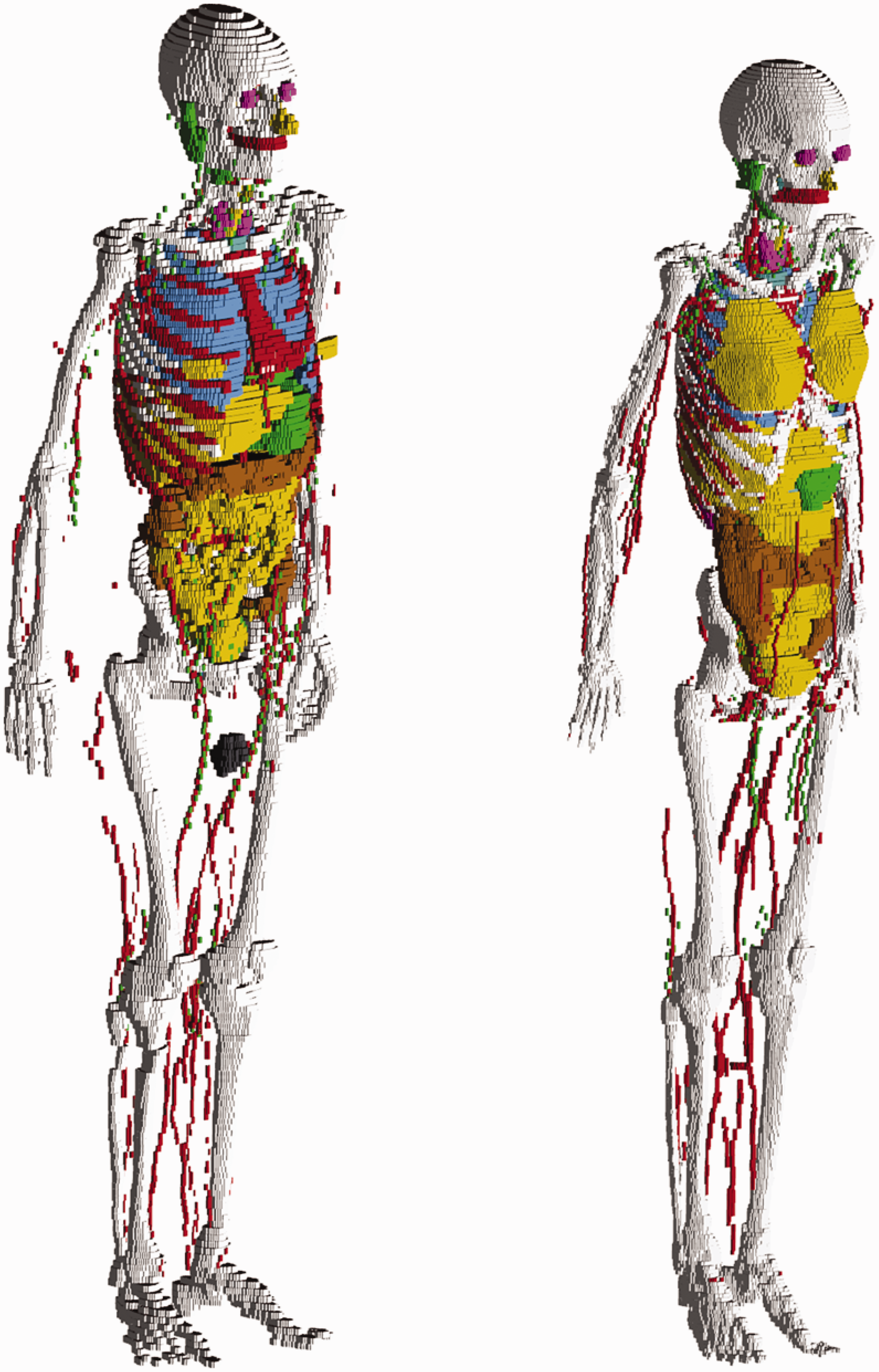
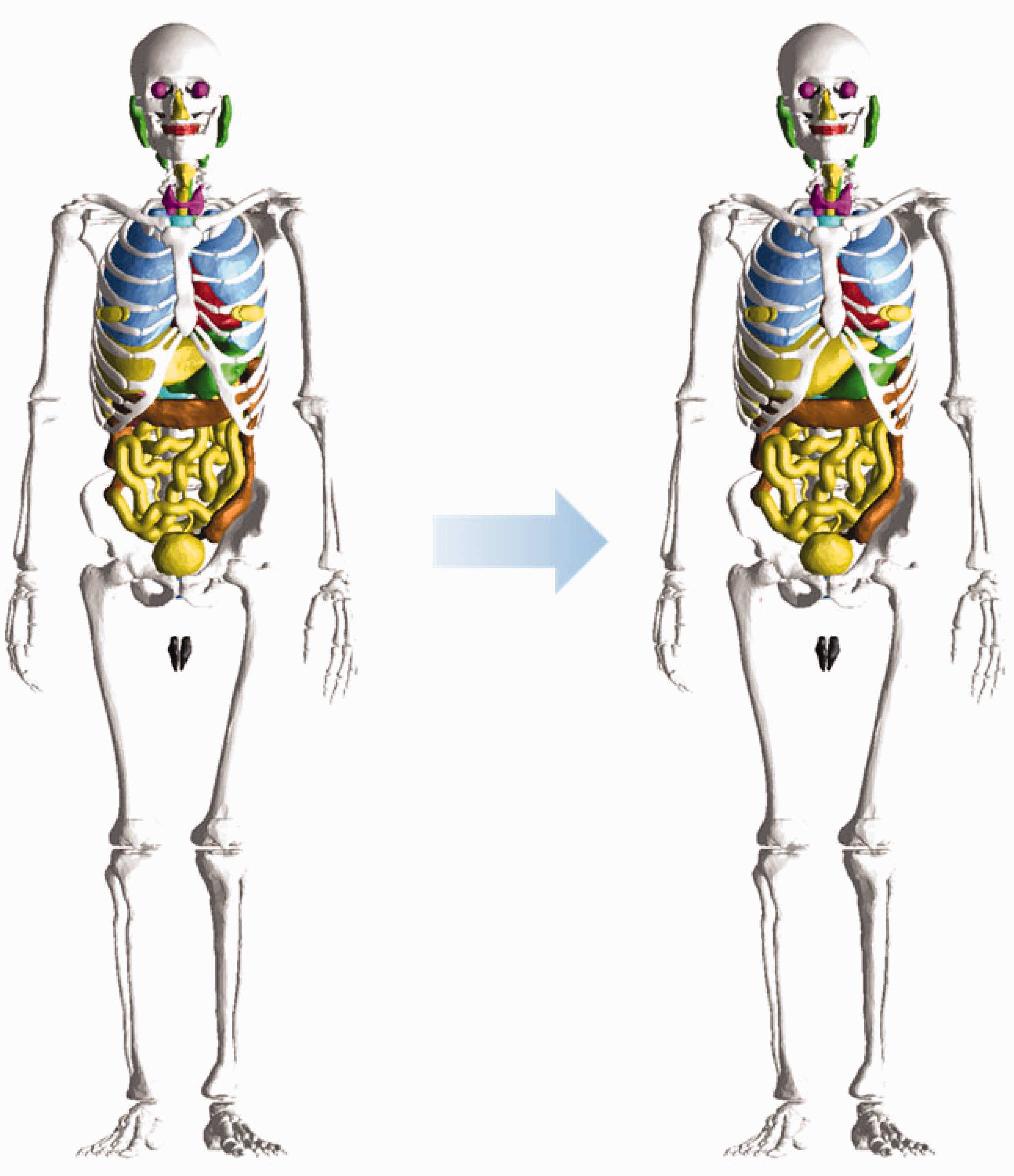
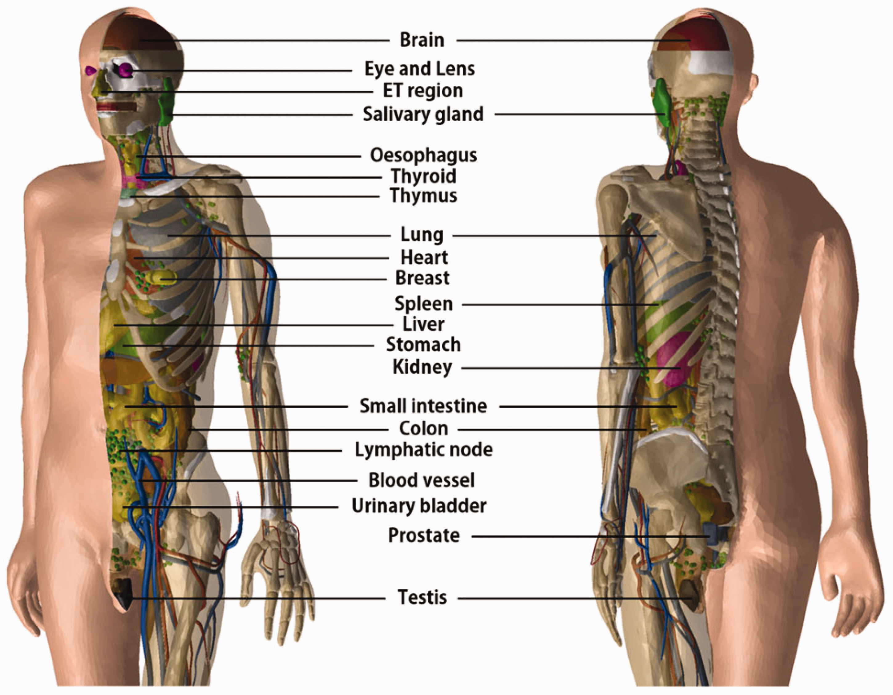
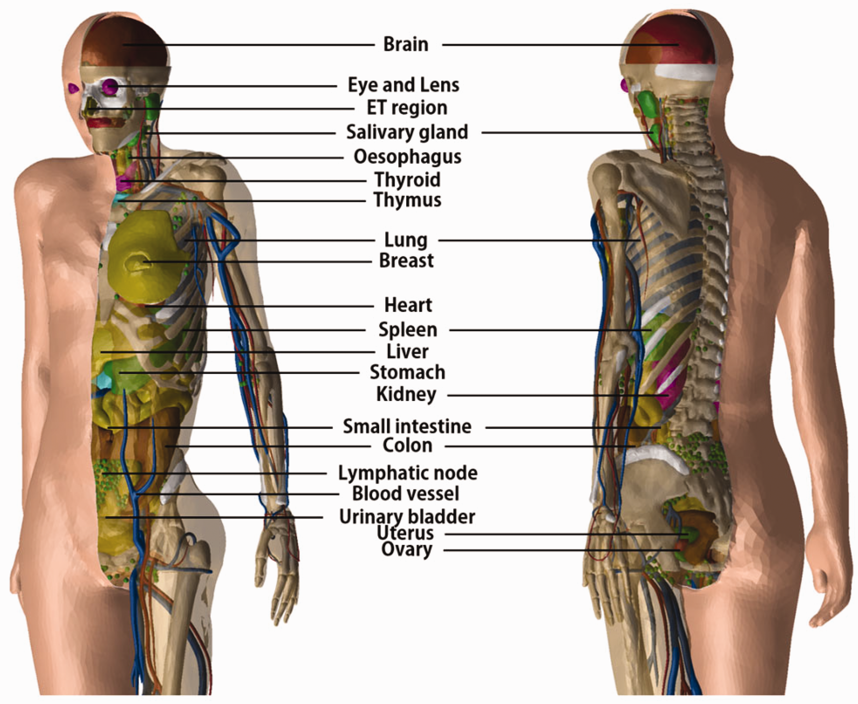
(25) The adult voxel-type reference computational phantoms described in Publication 110 (ICRP, 2009) were adopted by ICRP and ICRU as the phantoms for computation of the ICRP/ICRU reference DCs for radiological protection purposes. These computational phantoms are digital 3D representations of the human anatomy, constructed using CT images of real people. The phantoms are consistent with the information given in Publication 89 (ICRP, 2002) on the reference anatomical parameters of Reference Adult Male and Reference Adult Female. The Publication 110 phantoms are shown in Fig. 2.1. (26) While providing more anatomically realistic representations of internal anatomy than the older type of stylised phantoms, the adult voxel-type reference phantoms have limitations due to their voxel resolution, and hence some organs and tissues could not be represented explicitly or could not be adjusted to their reference mass due to their small dimensions or complex anatomical structure. This fact was discussed in Publication 110 (ICRP, 2009). In an attempt to address the limitations of the voxel-type reference phantoms related to image resolution, further improvements in representing these organs and tissues were made in the adult MRCPs described in the present publication. These improvements are summarised in the following paragraphs. (27) The skin of the voxel-type reference phantoms is represented by a single voxel layer, considering only transverse directions, resulting in the skin being discontinuous between individual transverse slices. The total skin mass of the phantoms is 13% and 18% higher than the reference values for the adult male and female, respectively. Through the discontinuous parts of the skin, radiation incident at non-zero angles of incidence relative to the transverse slices can reach internal organs or tissues (e.g. breasts, testes, and salivary glands) directly without first penetrating the skin layer. This might lead to an overestimation of DCs for weakly-penetrating radiations incident at angles that are not perpendicular to the body length axis. The MRCPs, in contrast, are fully wrapped by the skin, whose total mass is in accordance with the reference value. Note that other organs and tissues with thin tissue structures (such as gastrointestinal tract organs and cortical bone) are discontinuous in the voxel-type reference phantoms; this issue is resolved fully within the MRCPs. (28) The small intestine of the voxel-type reference phantoms, in addition to showing discontinuous parts, does not represent its complex tubular structure precisely. Therefore, high-quality small intestine models were incorporated into the MRCPs, whereby models were generated using a dedicated procedure based on a Monte Carlo sampling approach (Yeom et al., 2016a). Similarly, high-quality detailed models of the spine (cervical, thoracic, and lumbar) and hand and foot bones were incorporated into the MRCPs (Yeom et al., 2016b). (29) The lymphatic nodes of the voxel-type reference phantoms were drawn manually at locations specified in anatomical textbooks (Brash and Jamieson, 1943; Möller and Reif, 1993, 1997; GEO kompakt, 2005) because they could not be identified on the original CT images. Although the higher concentration at specific locations (e.g. groin, axillae, hollows of the knees, crooks of the arms) described in the textbooks was incorporated correctly into the Publication 110 (ICRP, 2009) phantoms, site-specific numbers of the lymphatic nodes presented in Publication 89 (ICRP, 2002) were not considered. In the MRCPs, lymphatic nodes were regenerated by a modelling approach used for the University of Florida and the National Cancer Institute (UF/NCI) family of phantoms (Lee et al., 2013) based on the lymphatic node data derived from the data of Publications 23, 66, and 89 (ICRP, 1975, 1994a, 2002) (see Section 3.4). (30) The complex structure of the eye could not be represented precisely in the voxel-type reference phantoms due to the image resolution. Therefore, the detailed eye model of Behrens et al. (2009) was adopted in Publication 116 (ICRP, 2010), and the lens DCs of Publication 116 were calculated using either the voxel-type reference phantoms or the adopted eye model, depending on radiation type, energy, and irradiation geometry. In order to be able to compute the absorbed dose to the lens of the eye using only one anthropomorphic phantom for each sex, the detailed eye model of Behrens et al. (2009) was incorporated directly into the MRCPs (Nguyen et al., 2015). (31) The Commission recommended that a range from 50 to 100 µm below the skin surface should be considered as an appropriate depth for the basal cell layer of most body regions of the skin (ICRP, 1977, 2010, 2015). The 50-µm-thick radiosensitive skin layer, however, cannot be represented in the voxel-type reference phantoms due to their limited voxel resolution. The skin DCs of Publication 116 (ICRP, 2010) for external exposures were thus calculated by averaging the absorbed dose over the entire skin of the phantoms. This approximation is acceptable for the calculation of effective doses for penetrating radiations, considering the small tissue weighting factor of the skin (wT = 0.01). However, for weakly-penetrating radiations, such as alpha and beta particles, this approximation leads to underestimations or overestimations in skin target cell layer doses. In the skin of the MRCPs, the 50-µm-thick radiosensitive target layer was defined explicitly. (32) Similarly, the micrometre scales of radiosensitive tissues and source regions for radionuclide retention of the respiratory and alimentary tract systems, as described in Publications 66 and 100 (ICRP, 1994a, 2006), could not be represented in the voxel-type reference phantoms. Separate stylised models, describing the respiratory and alimentary tract organs as mathematical shapes (e.g. a sphere or a right circular cylinder), were used for the calculation of SAFs for charged particles (ICRP, 1994a, 2006, 2016). In the MRCPs, the micrometre-thick target and source regions in the alimentary and respiratory tract systems as described in Publications 66 and 100 (ICRP, 1994a, 2006) were included (Kim et al., 2017). Realistic lung airway models that represent the bronchial (BB) and bronchiolar (bb) regions were also developed and incorporated into the MRCPs, whereas in the voxel-type reference phantoms, the bronchi could not be followed down to more than the very first generations of airway branching (Kim et al., 2017). Furthermore, the bronchioles are too small to be represented in a voxel basis (ICRP, 2009). (33) Previously, the organ and tissue masses of computational anthropomorphic phantoms (Lee et al., 2007; ICRP, 2009; Yeom et al., 2013) were commonly adjusted to the reference values listed in Table 2.8 of Publication 89 (ICRP, 2002). However, these masses correspond to the masses of organ/tissue parenchyma alone, while the optimal phantom design would provide organ volumes consistent with both the organ parenchyma and included blood vasculature. In a living person, on the other hand, a large proportion of blood is distributed in small vessels and capillaries within the organs and tissues, thus slightly increasing the organ and tissue masses within the phantom body. In recognition of this circumstance, target tissue/organ masses inclusive of blood were used to calculate the self-irradiation SAFs of Publication 133 (ICRP, 2016). To reflect this in the new MRCPs, the organ and tissue masses and tissue compositions of these phantoms were adjusted to include their organ blood content. The blood distribution among the organs and tissues was derived from the reference regional blood volume fractions given in Publication 89 (ICRP, 2002) using an approach similar to that outlined in Publication 133 (ICRP, 2016). The voxel-type reference phantoms of Reference Adult Male (left) and Reference Adult Female (right). The skin, muscle, and adipose tissue are not displayed in this figure.
3. CONVERSION OF THE ADULT VOXEL-TYPE REFERENCE PHANTOMS TO MESH FORMAT
3.1. Simple organs and tissues
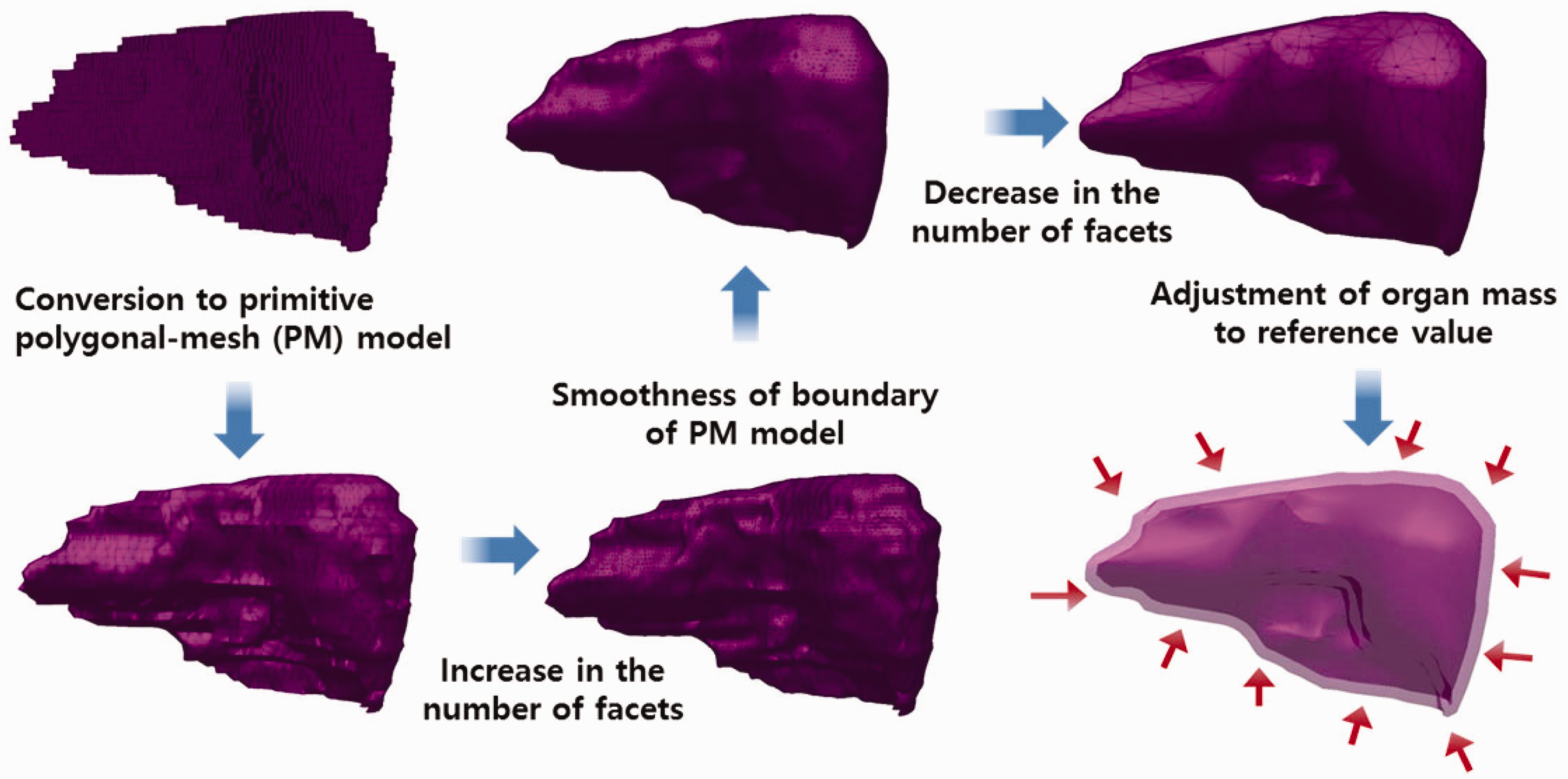
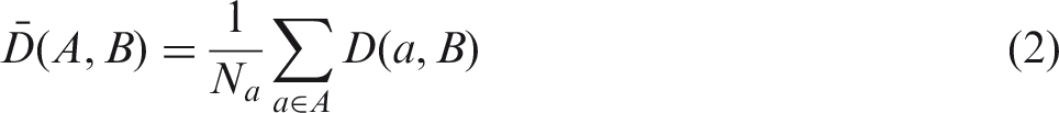
(34) Most organs and tissues in the MRCPs were constructed by directly converting the adult voxel-type reference phantoms to the PM format via 3D surface rendering and subsequent refinement procedures. Fig. 3.1 describes the procedure schematically. The voxel data of the phantoms were imported into 3D-DOCTOR (Able Software Corp., Lexington, MA, USA). The organs and tissues were then contoured using the ‘Interactive Segmentation’ command of the software. The contoured lines were converted to primitive PM models using the ‘Surface Rendering’ command. These primitive PM models, generally showing some stair-stepped surfaces with holes and defects, were refined into high-quality PM models using Rapidform (INUS Technology Inc., Seoul, Korea). In order to minimise distortion of the original shape during the refinement process, the number of facets was increased using the ‘Subdivide’ command of the software. The PM models were smoothed with the ‘Smooth’ command, and their holes and defects were eliminated using the ‘Fill Holes’ and ‘Healing Wizard’ commands. Subsequently, the number of polygonal facets was reduced to a reasonable number by applying the ‘Decimate’ command repeatedly. Finally, the refined PM models were adjusted to match Publication 89 reference masses (ICRP, 2002) using the ‘Deform’ command. For the organs and tissues including inner structures such as hollow organs, the refined PM models were replicated to produce separate models to define inner structures. The sizes of the inner structure models were then reduced by adjusting their volumes to match the target mass using the ‘Offset’ and ‘Deform’ commands. For some complex organs such as the colon, the voxels were first converted to NURBS models and then to PM models. (35) Note that the reference value for the oesophageal contents is not given in Publication 89 (ICRP, 2002); thus, the Publication 110 (ICRP, 2009) phantoms do not include the oesophageal contents, which makes it impossible to calculate SAFs for the oesophagus for radiations emitted by ingested radioactive material during passage through the oesophagus. In the MRCPs, therefore, the oesophageal contents were added as part of the oesophagus, having the same volume as the Publication 100 (ICRP, 2006) stylised models (male 22.0 cm3, female 20.4 cm3). For this change, both the length and diameter of the original voxel-type oesophagus had to be increased by ∼0.3 cm. Resultantly, the mass of the residual soft tissue (RST) was decreased in order to keep the body mass unchanged. RST is discussed in detail in Section 4.3. (36) During inclusion of the oesophageal contents, it was found that in the Publication 110 (ICRP, 2009) phantoms, the oesophagus contacts the thyroid for both the male and female phantoms, and the thyroid contacts the thymus for the male phantom, which are anatomically incorrect. These organs were separated in the MRCPs. (37) Due to the limited voxel resolution of the original voxel-type reference computational phantoms, it was impossible to properly segment the blood in the lungs of the Publication 110 (ICRP, 2009) phantoms. Consequently, blood mass (male 150 g, female 101 g) is significantly less than the reference value (male 700 g, female 530 g), and unsegmented blood is included implicitly in the lung tissue (ICRP, 2009). In the PM model of the lungs, the segmented blood was included in the lung tissue by recalculating the density and elemental composition of the lung tissue. This approach increased lung density by 8.6% (male) and 7.3% (female). These changes will not significantly affect calculated absorbed doses to the lungs. (38) During the conversion process, the PM models were adjusted to the voxel models, monitoring two indices which show the geometric similarity between two given objects. The first index used in the process was the Dice index (DI), which simply represents the volume overlap fraction of two objects (Dice, 1945). For confirmation of successful adjustment, it was considered that the DI value should be >95% of the maximum achievable Dice index (MADI) for a given organ. Note that MADI exists for a given organ due to the fundamental difference in the geometry format (i.e. voxel vs PM), which was estimated by calculating the DI value between the PM model under adjustment and its voxelised model with the same voxel resolution as the Publication 110 (ICRP, 2009) phantoms. The second index is the centroid distance (CD), which is the distance between the centroids of the voxel model and the corresponding PM model. It was considered that the CD value should be <0.5 mm for confirmation of a successful adjustment. (39) CD values were <0.5 mm for all organs and tissues which were converted directly from the Publication 110 (ICRP, 2009) voxel models. The DI values were greater than the target DI (=95% of MADI) for most organs and tissues, but there were some exceptions. For the oesophagus, for example, the DI value was less than the target DI value because the total volume of the oesophagus of the PM models was increased intentionally in order to include the oesophageal contents, as discussed above. A few other organs and tissues also showed low DI values because the finite voxel resolution resulted in disconnections of these organs in the Publication 110 phantoms. For the PM models, the disconnected organ/tissue was first connected and then adjusted to maximise the DI value. After completion of conversion, an additional geometric similarity index, the Hausdorff distance (HD) (Hausdorff, 1918), was calculated, defined as:
Conversion procedure applied for most organs and tissues. Lymphatic node numbers and masses for Reference Adult Male and Reference Adult Female derived from the data of Publications 23, 66, and 89 (ICRP, 1975, 1994a, 2002), along with reference node numbers given in Publication 89 (ICRP, 2002).

3.2. Skeletal system
(40) Most bones [i.e. upper arm bones (humeri), lower arm bones (ulnae and radii), clavicles, upper leg bones (femora), lower leg bones (tibiae, fibulae, and patellae), mandible, pelvis, scapulae, sternum, cranium and ribs] were produced using the same conversion procedure employed for the single-region organs and tissues, as demonstrated above for the liver. For the spine (cervical, thoracic, and lumbar), which is a very complicated tissue structure, a set of existing high-quality PM models produced from serially sectioned colour photographic images of cadavers (Park et al., 2005) was taken and adjusted to the voxel models, monitoring both DI and CD values. Similarly, for the hands and feet, a set of high-quality PM models produced from micro-CT data of cadavers (http://dk.kisti.re.kr) was adopted; these models were not adjusted to the voxel models but simply scaled to match the target masses and then placed at the ends of the arms and legs of the MRCPs. Note that in the Publication 110 (ICRP, 2009) female phantom, the feet are inclined (because the original subject was imaged under CT in a prone position). In the MRCP, the feet were re-oriented in a flat, standing position such as found in the Publication 110 male phantom. (41) In the Publication 110 (ICRP, 2009) phantoms, the cartilage was not fully segmented, mainly due to low contrast in the original CT data. In the MRCPs, the costal cartilage and intervertebral discs were also modelled following the method used for construction of the UF/NCI phantoms (Lee et al., 2010). To maintain the reference cartilage mass, the remaining cartilage was simply included in RST, which is discussed in Section 4.3. Strictly speaking, this approach is equally incorrect as the approach used in the Publication 110 phantoms in which the non-segmented cartilage was included in the spongiosa regions. However, the present approach is more acceptable dosimetrically, considering that the density and effective atomic number of the cartilage are close to those of soft tissues and that the cartilage is neither a radiation-sensitive tissue nor a frequent source region for internal dosimetry; the exact location and distribution of the remaining cartilage is thus not important from the dosimetric point of view. (42) The sacrum of the Publication 110 (ICRP, 2009) female phantom lacks cortical bone due to limitations with voxel resolution; therefore, cortical bone was added to the sacrum of the female phantom, assuming that the female cortical bone mass fraction is identical to that of the male. To maintain the total cortical bone mass unchanged, the cortical bone of the female lower leg bones was reduced considering that the cortical bone mass fraction of the female lower leg bones (19%) was significantly higher than that of the male lower leg bones (12%). More detailed information on the skeleton conversion can be found in Yeom et al. (2016b). (43) Note that in the skeletal system, the micron-scale structures of the skeletal target tissues (i.e. active bone marrow and skeletal endosteum) are not modelled and, therefore, the dose to these skeletal tissues needs to be calculated using fluence-to-dose–response functions, such as those presented and described in Annexes D and E of Publication 116 (ICRP, 2010). Flowchart of program developed to generate lymphatic nodes in the polygon mesh phantoms.
3.3. Small intestine
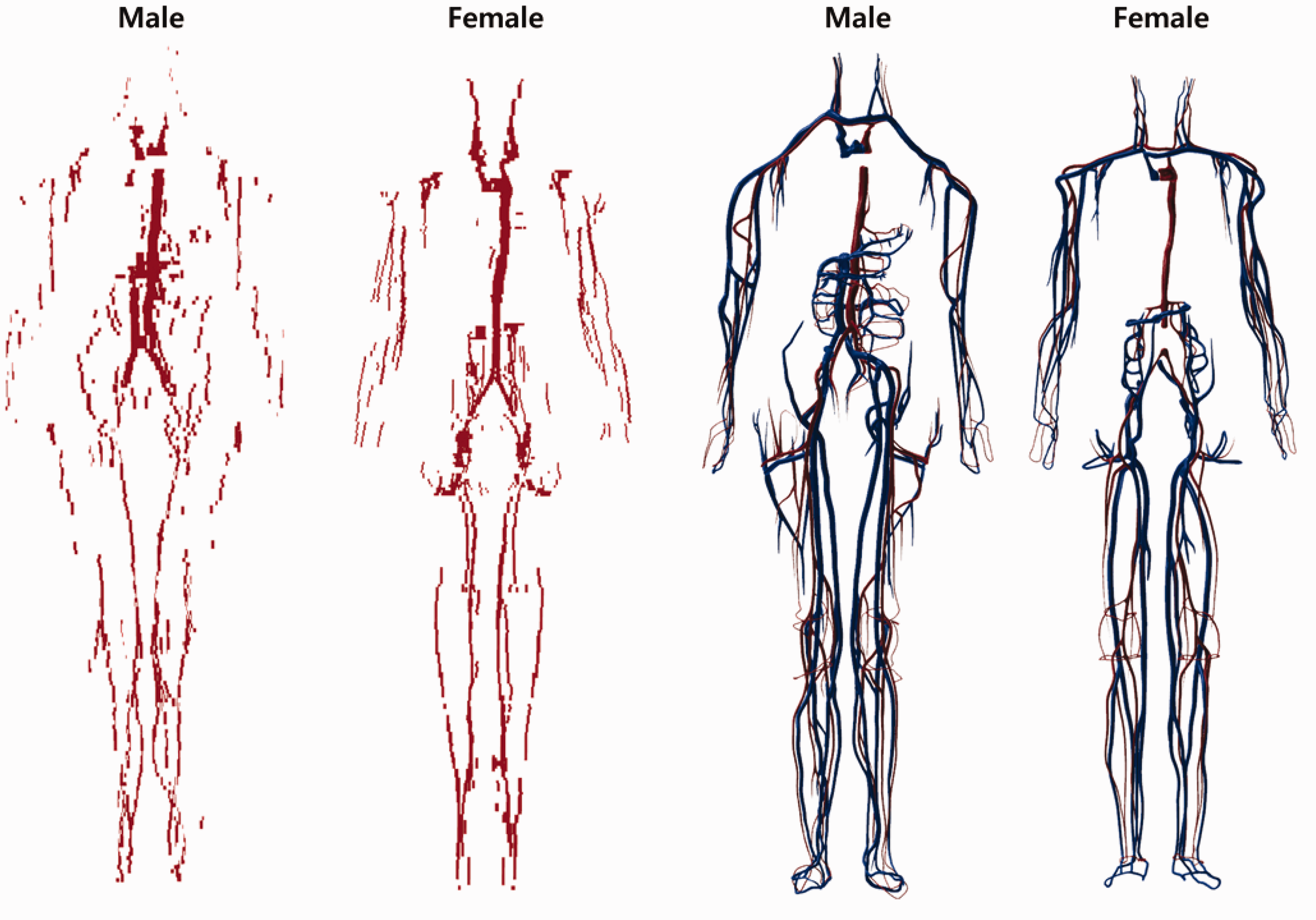
(44) The small intestine was not represented precisely in the Publication 110 (ICRP, 2009) phantoms, mainly because its complex tubular structure was not clearly distinguishable in the original cross-sectional CT data and its modelling was limited due to the finite voxel resolution. Accordingly, a dedicated procedure and a computer program were used to generate the small intestine models in the MRCPs (Yeom et al., 2016a). First, a surface frame, entirely enclosing the original small intestine voxel model, was constructed using the alpha-shape algorithm (Edelsbrunner et al., 1983). Next, a dedicated computer program developed in C++ was used to generate a small intestine passage line using a Monte Carlo sampling approach. Along with the passage line, a PM-format small intestine model was generated, whose masses of the wall and contents were matched to the reference values given in Publication 89 (ICRP, 2002). The aforementioned procedure was repeated to produce 1000 different small intestine models, with the best model selected considering both its geometric and dosimetric similarity. More detailed information on construction of the small intestine model can be found in Yeom et al. (2016a). Blood in large vessels of the Publication 110 (ICRP, 2009) phantoms (left) and the mesh-type reference computational phantoms (MRCPs) (right). In the MRCPs, the red colour indicates the blood in the large arteries and the blue colour indicates the blood in the large veins.
3.4. Lymphatic nodes
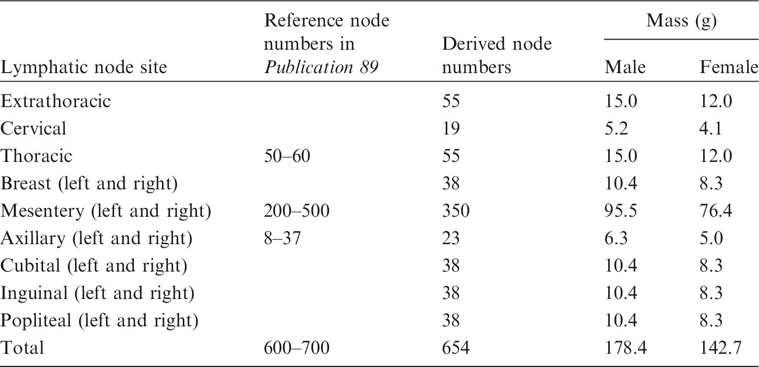
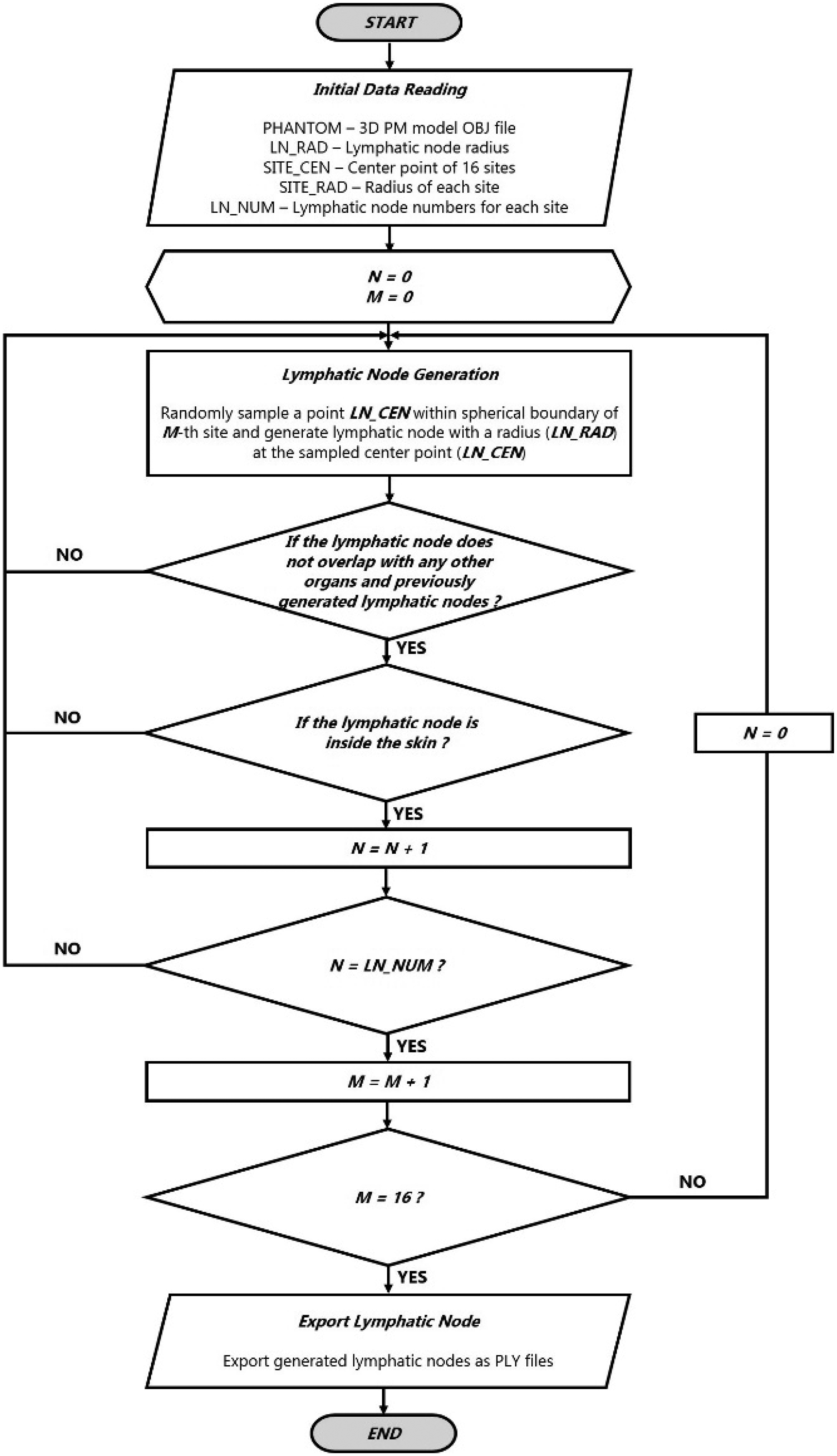
(45) The lymphatic nodes of the Publication 110 (ICRP, 2009) phantoms could not be converted directly to the PM format due to their complexity and distributed nature in the body. The lymphatic nodes in the PM format were therefore generated using a similar modelling approach as used to generate lymphatic nodes in the UF/NCI phantoms (Lee et al., 2013) based on the lymphatic node data (see Table 3.1), which were derived from the data of Publications 23, 66, and 89 (ICRP, 1975, 1994a, 2002). Note that the derived lymphatic node data are consistent with the values adopted for the calculations of Publication 133 (ICRP, 2016). For generation of the lymphatic nodes, a dedicated computer program was developed following the procedure shown in Fig. 3.2. The program first loads the initial data: (1) the PM phantom data; (2) the single-node PM data; (3) the nodal diameter; (4) the coordinates of the lymphatic node sites; (5) the diameters of the spherical clusters for the sites; and (6) the site-specific nodal numbers. Next, the program generates lymphatic nodes satisfying the following two criteria at random: (1) a node should be placed within the corresponding cluster sphere; and (2) a node should not overlap other organs and tissues, or the previously generated nodes. The procedure is repeated until the number of generated nodes reaches a predefined number.
3.5. Eyes
(46) The Publication 110 (ICRP, 2009) phantoms, due to their voxel sizes on the order of a few millimetres, do not properly represent the detailed structure of the eye. The lens DCs of Publication 116 (ICRP, 2010) on idealised external radiation exposures were therefore calculated using either the Publication 110 phantoms or the detailed stylised eye model developed by Behrens et al. (2009), depending on radiation type, energy, and irradiation geometry. To avoid this situation, the detailed eye model of Behrens et al. (2009) was incorporated directly into the male and female MRCPs. First, using the geometric information of Behrens et al.’s detailed eye model, a NURBS-format eye model was produced and then converted to the PM format. Defects in the converted model were repaired using the refinement functions of Rapidform (INUS Technology Inc.). Finally, the PM eye model was placed in the MRCPs, matching the centroid of the eye of the Publication 110 phantoms. More detailed information on the eye model can be found in Nguyen et al. (2015).
3.6. Blood in large vessels
(47) Only the blood in the large blood vessels is modelled in the Publication 110 (ICRP, 2009) phantoms, again due to the limited resolution of the original CT image data (8- and 5-mm slice thicknesses for the male and female phantoms, respectively). Consequently, the mass of the segmented blood in the Publication 110 phantoms (male 371 g, female 384 g) is significantly less than their corresponding reference values (male 1344 g, female 984 g). This issue was addressed in the MRCPs. For the MRCPs, first, the blood of the large blood vessels was converted to the PM format, whose mass was then matched to the reference value. For this step, the blood models of the Publication 110 phantoms were first converted to primitive PM models using a surface rendering method in 3D-DOCTOR (Able Software Corp.). Next, the contour lines were generated carefully along the blood passages identified in the primitive PM models using the ‘Section’ command of Rhinoceros (Robert McNeel & Associates, Seattle, WA, USA). The generated contour lines were then used to generate NURBS surfaces using the ‘Loft’ command of the software. Finally, the NURBS surfaces were converted to the PM format using the ‘Mesh’ command. In the MRCPs, the remaining part of the blood in the smaller blood vessels was modelled manually with the NURBS modelling tools of Rhinoceros, referring to the high-quality 3D blood models provided by BioDigital (https://www.biodigital.com). The modelled NURBS surfaces were converted to the PM format, and then the converted PM models were connected to the PM models of the blood in the large vessels using the ‘Union’ command of Rapidform (INUS Technology Inc.). Finally, the combined PM models were adjusted to match the reference values using the ‘Deform’ command of the software. Fig. 3.3 shows the developed blood PM models, along with the Publication 110 blood voxel models. Note that the intra-organ vasculature is not modelled in the phantoms; that is, the blood in the large vessels stops at the surface of the organs, and the blood within the organs is assumed to be homogeneously mixed with the parenchyma of the organs.
3.7. Muscle
(48) The muscle of the PM models was constructed after completion of all internal organs and tissues. Most muscle (i.e. trunk, arms, and legs) was constructed by direct conversion and refinement, whereas the other complex parts (i.e. head, hands, and feet) were constructed by a modelling approach. For construction, a series of labour-intensive refinement work was involved to eliminate the defects and overlapping problems with other organs and tissues using the refinement tools of Rapidform (INUS Technology Inc.). In addition, the rear side of the muscle (back, hip, and calf), which had been flattened in the Publication 110 (ICRP, 2009) phantoms due to the lying position of the individual originally imaged under CT, was reshaped to produce the muscular shape present in a standing person.
4. INCLUSION OF BLOOD IN ORGANS AND TISSUES
(49) The organ/tissue masses of the MRCPs include their intra-organ blood content. This is not the case in the Publication 110 (ICRP, 2009) phantoms, in which the organ/tissue masses are based on reference values listed in Table 2.8 of Publication 89 (ICRP, 2002) which are the masses of organ/tissue parenchyma (i.e. exclusive of blood content). Note that a large portion of blood situated in the small vessels and capillaries is distributed in the organs and tissues. For the MRCPs, therefore, the organ/tissue masses and compositions inclusive of blood content for adult male and female were calculated based on the reference regional blood volume fractions given in Publication 89 (ICRP, 2002) and, accordingly, the MRCPs were adjusted in volume to include blood content in their organs and tissues. Note that Publication 133 (ICRP, 2016) also considered the target masses inclusive of blood content for the calculation of SAFs for self-irradiation.
4.1. Calculation of mass, density, and elemental composition of organs and tissues inclusive of blood content
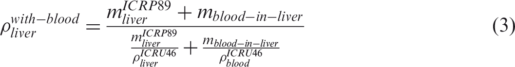
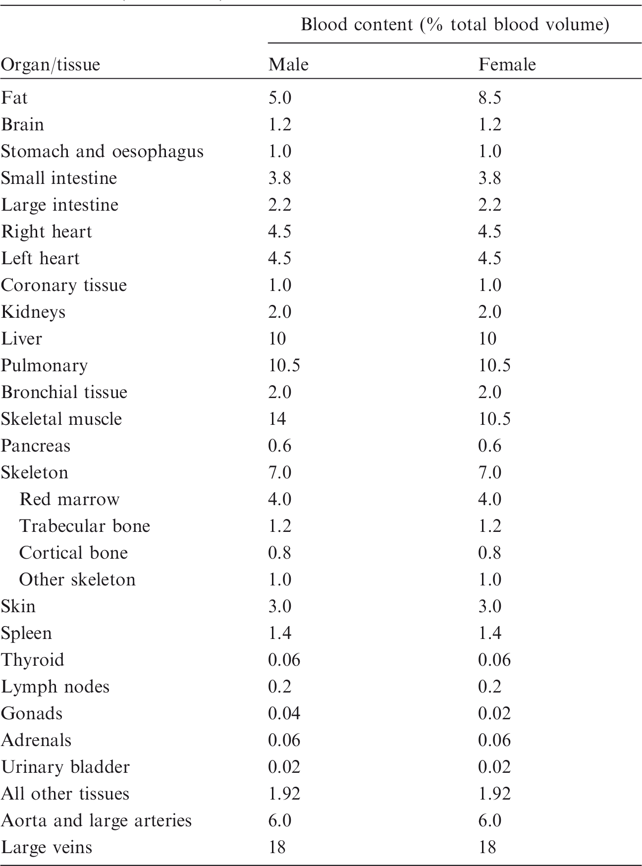
(50) Blood-inclusive organ/tissue masses, listed in Table 2.8 of Publication 89 (ICRP, 2002), were calculated using the reference values of regional blood volume fractions given in Table 2.14 of Publication 89 (ICRP, 2002), which is replicated in Table 4.1 below. There are organs and tissues whose reference blood fraction is given explicitly (i.e. fat, brain, stomach, oesophagus, small intestine, large intestine, right heart, left heart, coronary tissue, kidneys, liver, pulmonary, bronchial tissue, skeletal muscle, pancreas, active marrow, trabecular bone, cortical bone, other skeleton, skin, spleen, thyroid, lymph nodes, gonads, adrenals, and urinary bladder). Their blood-inclusive masses were calculated simply as the product of their reference blood fraction and the reference total body blood mass (adult male 5600 g, adult female 4100 g) given in Publication 89 (ICRP, 2002). (51) The reference blood fraction for the stomach and oesophagus is given as a single value, and thus not given separately as shown in Table 4.1; therefore, their blood mass was assigned in proportion to the organ mass under the assumption that the blood is distributed uniformly over these two organs. The same approach was used to calculate the blood mass of the inactive marrow, cartilage, teeth, and miscellaneous skeletal tissue, which are grouped as ‘other skeleton’ in Table 4.1. (52) In Table 2.8 of Publication 89 (ICRP, 2002), there are organs and tissues whose blood fractions are not listed explicitly in Table 2.14 of Publication 89 (ICRP, 2002); tongue, salivary glands, gallbladder wall, breasts, eyes, pituitary gland, larynx, trachea, thymus, tonsils, ureters, urethra, epididymis, prostate, fallopian tubes, uterus, and ‘remaining 4%’ tissues are represented by ‘all other tissues’ in Table 4.1. Note that ‘remaining 4%’ tissues indicate all of the organs and tissues that are not listed explicitly in Table 2.8 of Publication 89 (ICRP, 2002), which is approximately 4% of the body mass, mostly composed of separable connective tissues and certain lymphatic tissues. The blood mass of ‘all other tissue’ (male 107.5 g, female 78.7 g) was distributed to these organs and tissues in proportion to their masses. For this calculation, the mass of the ‘remaining 4%’ tissues was reduced due to extraction of the lymphatic nodes of which the mass (male 178.4 g, female 142.7 g) was adopted in Publication 133 (ICRP, 2016), considering that the reference blood fraction for the lymphatic nodes is given explicitly as shown in Table 4.1. The reference organ/tissue masses (exclusive of blood content) and the calculated blood-inclusive masses are given in Table 4.2. (53) After calculation of the blood masses, the densities and elemental compositions of the blood-inclusive organs and tissues were calculated using the data in Publication 89 (ICRP, 2002) and Report 46 (ICRU, 1992), again under the assumption that blood content is distributed uniformly over the organs and tissues. The density of the blood-inclusive liver, for example, was calculated using the following equation:
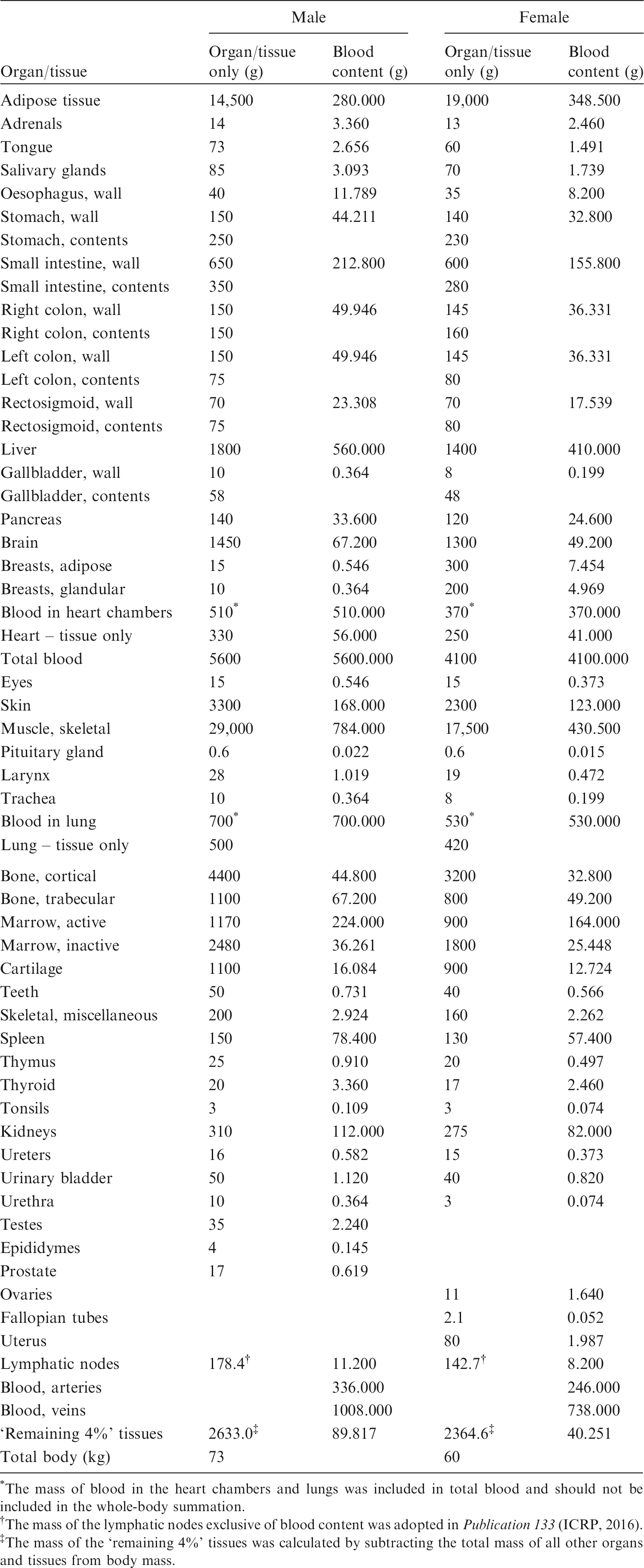
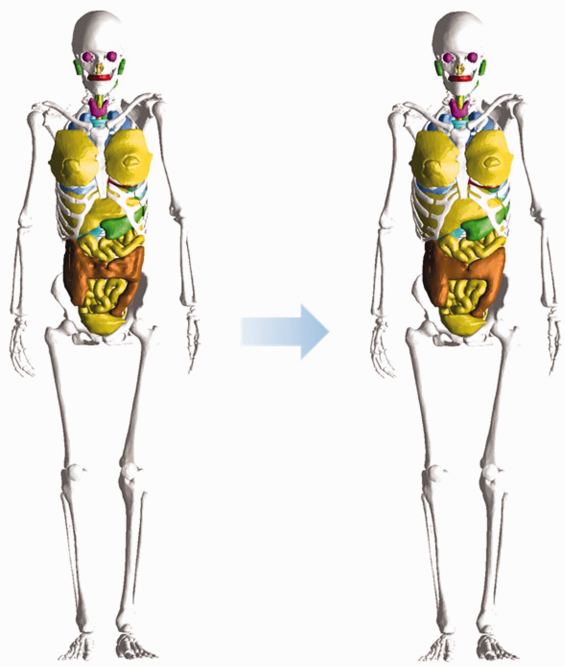
Reference values for regional blood volumes in adults given in Publication 89 (ICRP, 2002). Reference masses of organs and tissues for Reference Adult Male and Reference Adult Female. The mass of blood in the heart chambers and lungs was included in total blood and should not be included in the whole-body summation. The mass of the lymphatic nodes exclusive of blood content was adopted in Publication 133 (ICRP, 2016). The mass of the ‘remaining 4%’ tissues was calculated by subtracting the total mass of all other organs and tissues from body mass. Male phantom before (left) and after (right) adjustment for inclusion of blood content in organs and tissues.

4.2. Phantom adjustment for blood inclusion
(54) The PM models for all organs and tissues were subsequently adjusted to increase their volumes to allow for the volumetric inclusion of their blood content. The adjustment was performed using Rapidform (INUS Technology Inc.). Preferentially, the volumes of the organs and tissues were increased to match the blood-inclusive reference masses by globally enlarging a PM surface in the normal direction of the facets, which tends to maintain the centroid and original shape of the models. Among the increased organs and tissues, some overlaps were detected; the overlapping regions of the larger organs and tissues were preferentially eliminated rather than the smaller organs and tissues, in order to minimise distortion of the organ/tissue shapes. The organs and tissues with decreased volumes were adjusted manually to increase their volumes to match the reference masses, while at the same time monitoring the DI and CD values to minimise deformation of the organ shape from the original shape. (55) If there was insufficient space for the increase of the organ/tissue volumes, the organs and tissues were moved slightly to secure space. For example, the volume of the liver was increased significantly (i.e. >30% for both male and female), resulting in significant overlap problems with the adjacent organs and tissues, especially for the female mesh phantom. The lungs and ribs, therefore, had to be moved outward in the lateral direction by ∼2 mm and ∼4 mm for the male and female, respectively, after which the liver and adjacent organs and tissues were adjusted to match the reference masses without overlapping regions. (56) Figs 4.1 and 4.2 compare the internal organs and tissues of the MRCPs before and after inclusion of blood content for male and female, respectively. It can be seen that, in general, inclusion of blood content does not significantly change the topology of the phantoms. For detailed investigation to quantify geometric dissimilarity produced by blood inclusion, three similarity indices (DI, CD, and HD) were evaluated between the organs and tissues of the phantoms before and after their volumetric adjustment. (57) It was found that the CD and HD values were <∼2 mm for most organs and tissues. DI values were >0.8 for most organs and tissues. On the other hand, some organs and tissues were changed significantly due to blood inclusion. For the liver and kidneys, for example, CD and HD values ranged from 3.4 mm to 5.4 mm, and DI values ranged from 0.83 to 0.87; these differences are due to the fact that their mass was increased significantly by blood inclusion. In addition, some organs and tissues (such as ribs and spleen), located near the liver or kidneys, were changed significantly because they were moved to secure space for blood inclusion. Female phantom before (left) and after (right) adjustment for inclusion of blood content in organs and tissues.
4.3. Definition of residual soft tissue
(58) Although most organs and tissues in Table 4.2 are defined in the MRCPs, several organs and tissues (i.e. adipose tissue, larynx, urethra, epididymis, and fallopian tubes) are not included explicitly in the phantom anatomical structure. In contrast, several organs and tissues of the phantoms [i.e. main bronchi (=generation 1), spinal cord, urine, oesophageal contents, extrathoracic (ET) and inner air] are not listed in the table, but they can be considered as part of the ‘remaining 4%’ tissues in Table 4.2. In addition, the MRCPs only include costal and intervertebral cartilages, the total masses of which are significantly smaller than the reference values. (59) Despite these inconsistencies, the phantom mass should be consistent with the reference total body mass (male 73 kg, female 60 kg). This agreement was reached by defining an imaginary tissue, RST, in the MRCPs. RST implicitly includes all of the reference organs and tissues that are not defined explicitly in the phantoms: adipose tissue, larynx, cartilage (excluding costal and intervertebral cartilages defined in the phantoms), urethra, epididymis, fallopian tubes, and ‘remaining 4%’ tissue (excluding the organs and tissues defined in the phantoms but not listed in the reference values). (60) This approach has generally been used in the field of phantom development to match the phantom body mass to the reference body mass (ICRP, 2009; Lee et al., 2010; Kim et al., 2011; Yeom et al., 2013). In Publication 133 (ICRP, 2016), a similar approach was used to establish the source organ/tissue masses (see Table A.3 of Publication 133) for the purpose of use in the latest biokinetic models of the series of publications on occupational intakes of radionuclides (ICRP, 2015, 2017a,b). The established source organs/tissues do not include some reference organs/tissues, but the total mass of the source organs/tissues was matched to the reference body mass simply by increasing the adipose tissue mass. The increased adipose tissue plays the same role as RST defined in the MRCPs.
5. INCLUSION OF THIN TARGET AND SOURCE REGIONS
5.1. Skin
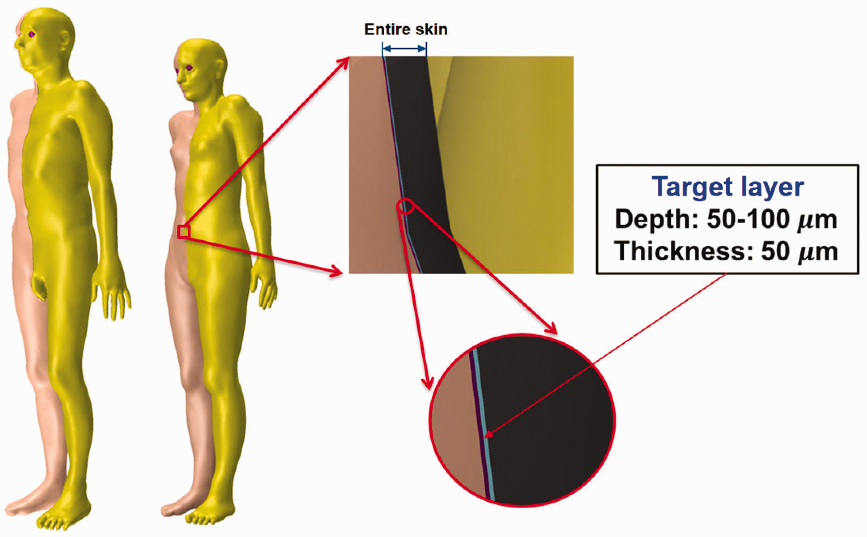
(61) The cells at risk in the skin are assumed to be in the tissue layer 50–100 µm below the skin surface (ICRP, 1977, 2010, 2015). However, the Publication 110 (ICRP, 2009) phantoms, due to their voxel resolution, do not have this thin target layer and consequently cannot be used for skin dose calculation for weakly-penetrating radiations (ICRP, 2010). In the MRCPs, the 50-µm-thick target layer was defined explicitly within the volume defining the total skin. (62) For this, first, the exterior surface of the skin was imported into Rapidform (INUS Technology Inc.) and then replicated to two additional surfaces. The sizes of the two surfaces were reduced to define the target layer within the skin at depths of 50 µm and 100 µm from the exterior skin surface, respectively, using the ‘Offset’ command of the software. Note that the ‘Offset’ command shrinks or enlarges a PM surface in the normal direction of the facets in the model, which allows the creation of surfaces to define the tens-of-micrometre-thick layer at a specific depth. Fig. 5.1 shows the skin of the MRCPs including the 50-µm-thick target layer. Skin of the MRCPs including the 50-µm-thick target layer: dead layer (purple colour), target layer (sky blue colour), and dermis layer (black colour).
5.2. Alimentary tract system
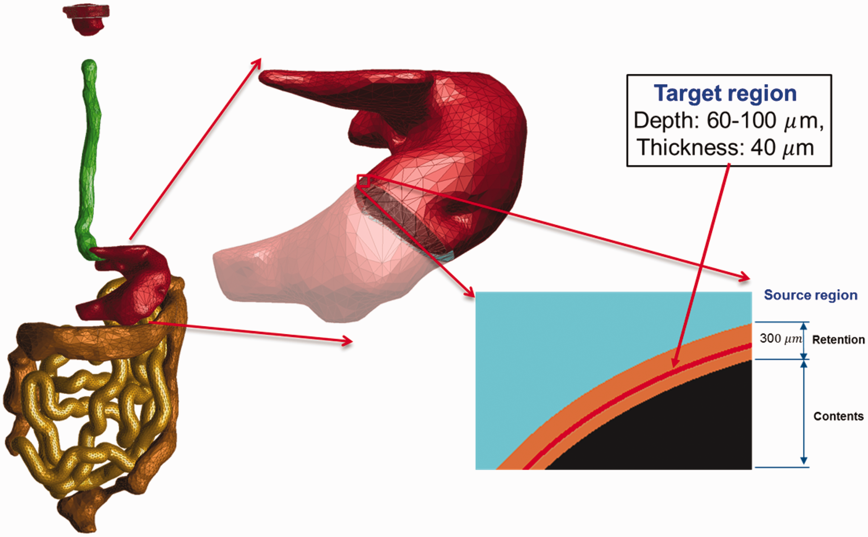
(63) The target regions (stem cell layers) and source regions (mucosal layers) of the alimentary tract organs (i.e. oral cavity, oesophagus, stomach, small intestine, and large intestine) were defined in the MRCPs according to the depth and thickness data for the target and source regions given in Publication 100 (ICRP, 2006). For all organs except the oral cavity, the thin target and source regions were simply defined using the ‘Offset’ command of Rapidform (INUS Technology Inc.) following the same method as used for the skin. Fig. 5.2 shows, as an example, the stomach of the male phantom including the target and source regions. (64) Note that the masses of the target regions (i.e. stem cells) for the stomach and intestines in the MRCPs do not exactly match those of the stylised models in Publication 100 (ICRP, 2006). For the stomach and large intestine, the difference in target mass between the mesh models and the stylised models is a natural consequence of their difference in the dimensions of the lumen, more specifically the surface area of the lumen to which the target mass is directly proportional. Note that, in the MRCPs, the stomach and large intestine were produced directly from the Publication 110 (ICRP, 2009) reference phantoms, in which the lumen is fully filled with the contents matching the reference value in Publication 89 (ICRP, 2002). For the small intestine, the difference in target mass is due to the high priority given to the reference values in Publication 89 (ICRP, 2002) throughout the construction of the MRCPs; that is, in the MRCPs, the mass of the contents was matched to the reference value in Publication 89 (ICRP, 2002). The diameter of the lumen, for which the reference value is not available, was not considered, resulting in a difference in target mass when compared with the stylised models in Publication 100 (ICRP, 2006). This approach is consistent with the Publication 110 reference phantoms in which the lumen of the small intestine is also fully filled with the contents matching the reference value in Publication 89 (ICRP, 2002). (65) In the oral cavity, two source regions were defined: source in food and source retained on the surface of the teeth. The food source volume (20 cm3) should be placed on the tongue, but in the Publication 110 (ICRP, 2009) phantoms, there was insufficient space to define the food source region; therefore, the tongue was divided into two parts – upper and lower – and the upper part was considered to be the food source region for the purpose of SAF calculation. The teeth-retained radionuclides were defined by adding a 10-µm layer to the surface of the teeth. The target layer in the oral mucosa was defined in three parts: tongue, roof of mouth, and lip and cheek. More detailed information on the alimentary tract system can be found in Kim et al. (2017). Alimentary tract organs (left) of the male mesh phantom and the enlarged view (right) of the stomach, including the target and source regions.
5.3. Respiratory tract system
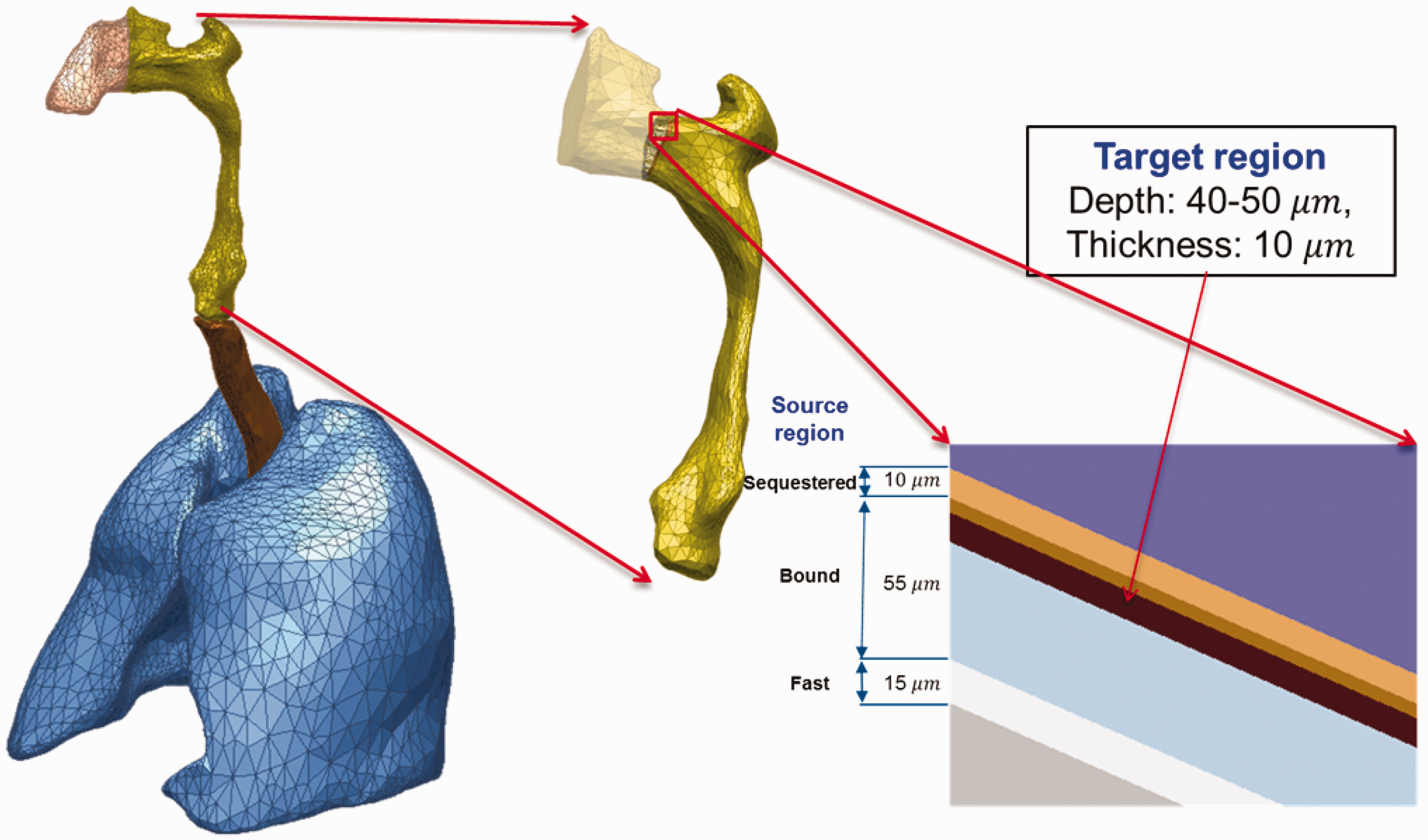
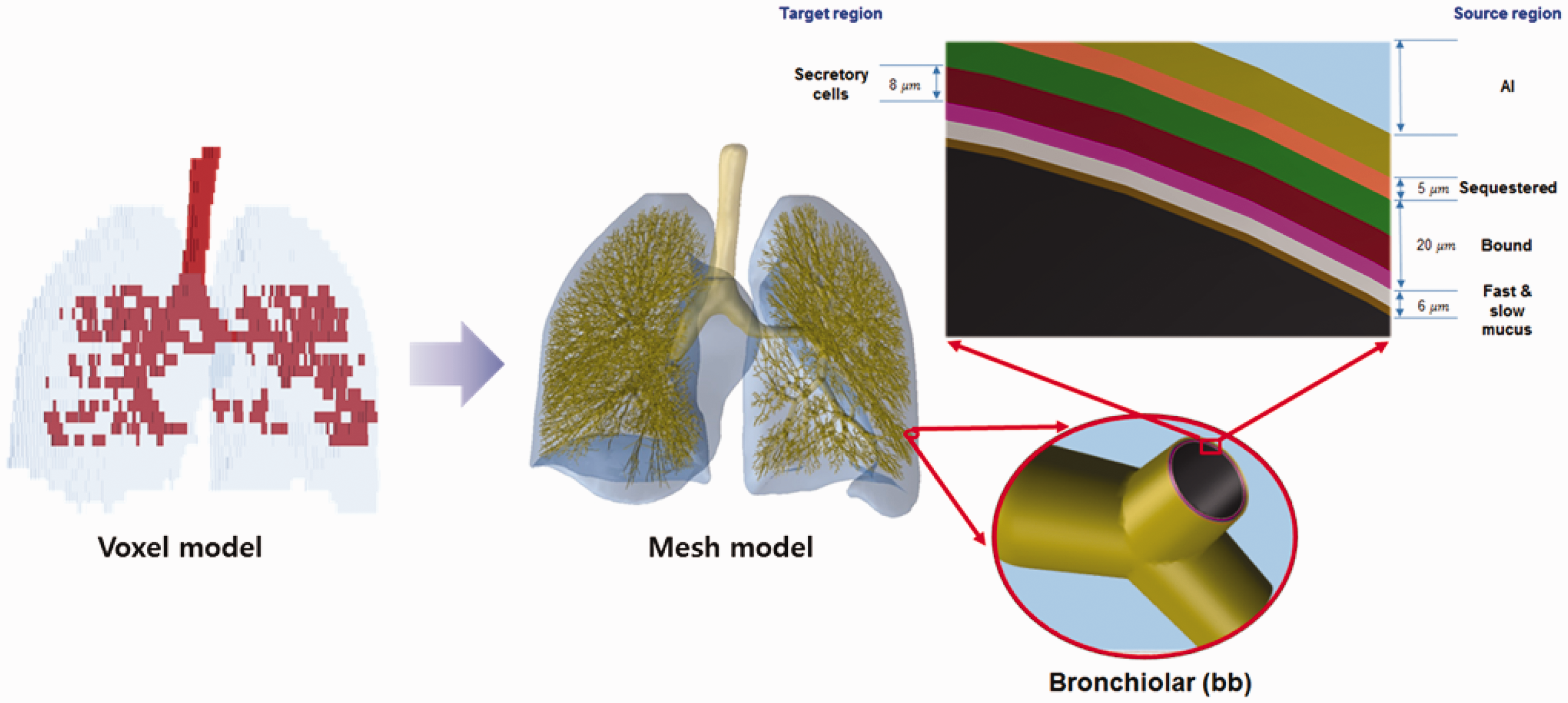
(66) The target and source regions of the respiratory tract organs were defined in the MRCPs following the morphometric data given in Publication 66 (ICRP, 1994a). The respiratory tract organs are composed of the extrathoracic regions (i.e. ET1 and ET2), BB, bb, and alveolar-interstitium (AI). The AI region was not defined separately but simply assumed to be distributed homogeneously within the lung tissue, except for the BB and bb regions, in the MRCPs, considering the statement of Publication 66 (ICRP, 1994a, Para. 313): ‘In the AI region, the interalveolar septa and the walls of blood and lymphatic capillaries are sufficiently thin to ensure that sensitive target cells are distributed homogenously throughout the tissue mass. Therefore, it can be assumed that the average dose received by the target cells is the same as that received by the whole tissue mass.’ (67) For the ET1 and ET2 regions, they were converted directly from the Publication 110 (ICRP, 2009) voxel models to a PM format, with their target and source regions defined using the ‘Offset’ command of Rapidform (INUS Technology Inc.) following the same method applied for the skin and alimentary tract organs. The same method was applied to the main bronchi (generation 1) that were converted directly from the Publication 110 voxel models to the PM format. Fig. 5.3 shows the ET2 region of the male phantom as an example, including both its Publication 66 (ICRP, 1994a) source and target regions. (68) The other generations (i.e. airway generations 2–8) of bronchi and all subsequent generations of bronchioles (i.e. airway generations 9–15) could not be converted from the Publication 110 (ICRP, 2009) voxel models; therefore, these airways were modelled using a dedicated computer program developed by Kim et al. (2017). The developed computer program generated branch-centre lines within the left and right lungs of the MRCPs based on a branching generation algorithm (Tawhai et al., 2000), following the diameter and length for each airway generation as given in Publication 66 (ICRP, 1994a). The branch-centre lines were used to construct airway models in the constructive solid geometry (CSG) format, whose models are based on an inverted Y-shape represented as a union geometry of spheres and truncated cones. The spheres, the diameters of which correspond to the branch diameters, are located at the ends of the branch-centre lines, and the truncated cones are located so as to be tangent to the mother and daughter spheres. The use of the inverted Y-shape model makes it possible to not only connect the surfaces of the neighbouring branches precisely but also to define the micrometre-thick source and target layers simply by changing the sphere diameters (i.e. branch diameters) (Lázaro Elias, 2011). (69) Note that the CSG-format airway models needed to be converted to the PM format for incorporation into the MRCPs. For this step, however, a large number of polygonal facets, eventually tetrahedrons, would be necessary to represent the airways properly, requiring a very large memory allocation (>∼50 GB), which is, at least at the present time, impractical. Therefore, a different approach was used for the airways; that is, the MRCPs were overlaid with the CSG lung airways in the Geant4 code (Agostinelli et al., 2003) using the G4VUserParallelWorld class, which is used for implementation of hierarchically overlapping multiple geometries called ‘parallel geometries’ (Apostolakis et al., 2008). This overlaying approach is currently only available in the Geant4 code, but enables dose calculation to be performed for the detailed CSG lung airways with minimal additional memory usage. (70) Fig. 5.4 shows the airway model produced for the lungs of the male phantom along with the original voxel model of the Publication 110 (ICRP, 2009) male phantom. The airway models of the MRCPs represent a complex tree structure, at the same time representing the thin target and source layers. The total lengths of the airway branches for each generation of the lung tree are in good agreement with their reference values; that is, the discrepancies are <10% for all generations. More detailed information on the respiratory tract system can be found in Kim et al. (2017). Respiratory tract organs (left) of the male mesh phantom and the enlarged view (right) of the ET2 region, including the target and source regions.
5.4. Urinary bladder
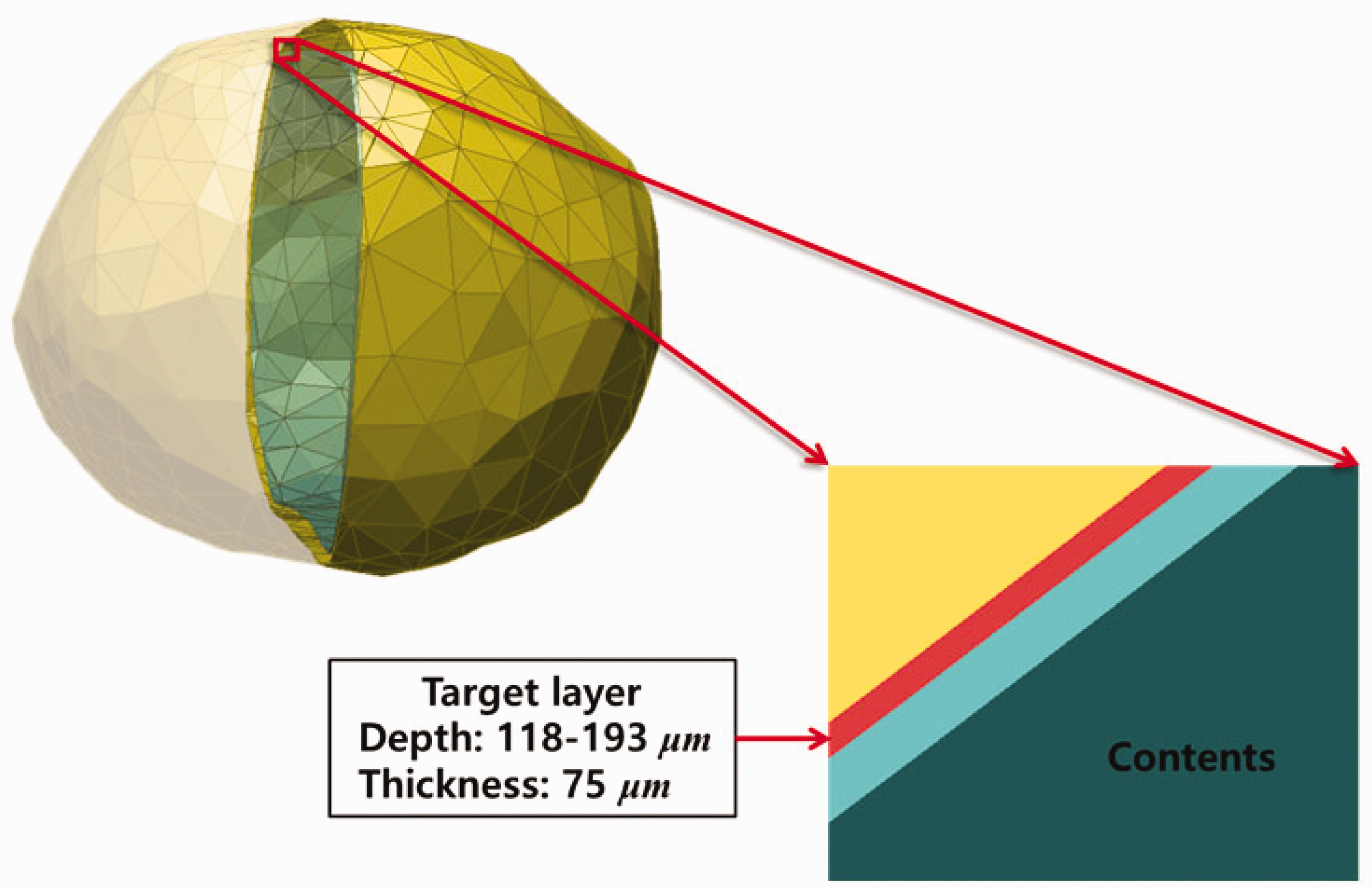
(71) The target layer of the urinary bladder was also defined in the MRCPs. In the urinary bladder, the basal cells of the epithelium are believed to be the relevant target cells at radiogenic risk (Colin et al., 2009), but doses have previously been calculated to the whole wall of the bladder (ICRP, 2016). Eckerman and Veinot (2018) derived the depth and thickness of the basal cell layer of the urinary bladder as 118 µm and 75 µm, respectively, for the adult male and 116 µm and 69 µm, respectively, for the adult female, assuming a constant and reference urine volume of 200 cm3 for both phantoms. In the MRCPs, these values were adopted to define the target layer in the urinary bladder, again using the ‘Offset’ command of Rapidform (INUS Technology Inc.). Fig. 5.5 shows the urinary bladder of the male mesh phantom including the target layer. Lung voxel model (left) and lung mesh model (right) for the male phantom (Kim et al., 2017). Urinary bladder of the male mesh phantom including the target layer (red).
6. DESCRIPTION OF THE ADULT MESH-TYPE REFERENCE PHANTOMS
6.1. General phantom characteristics
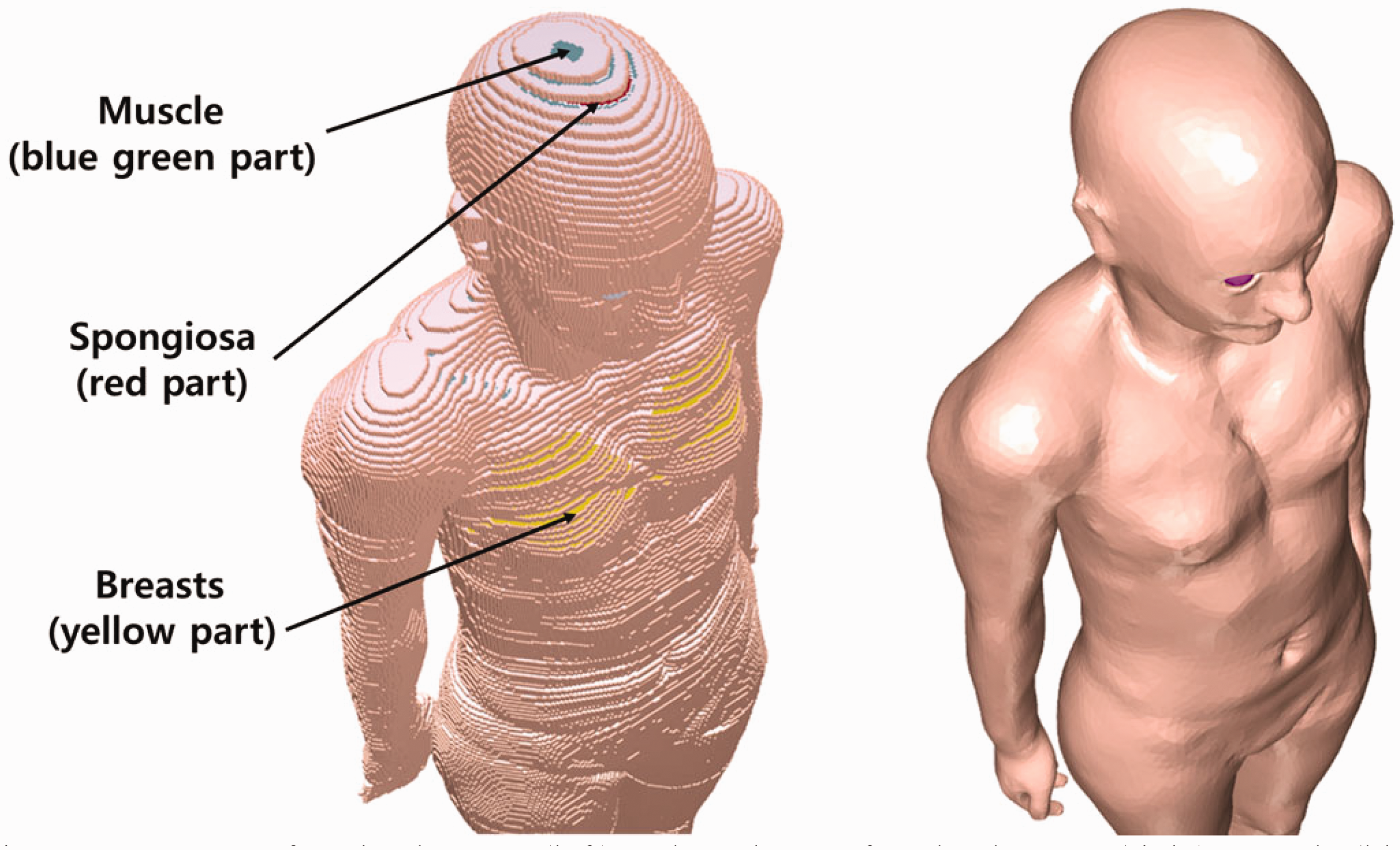
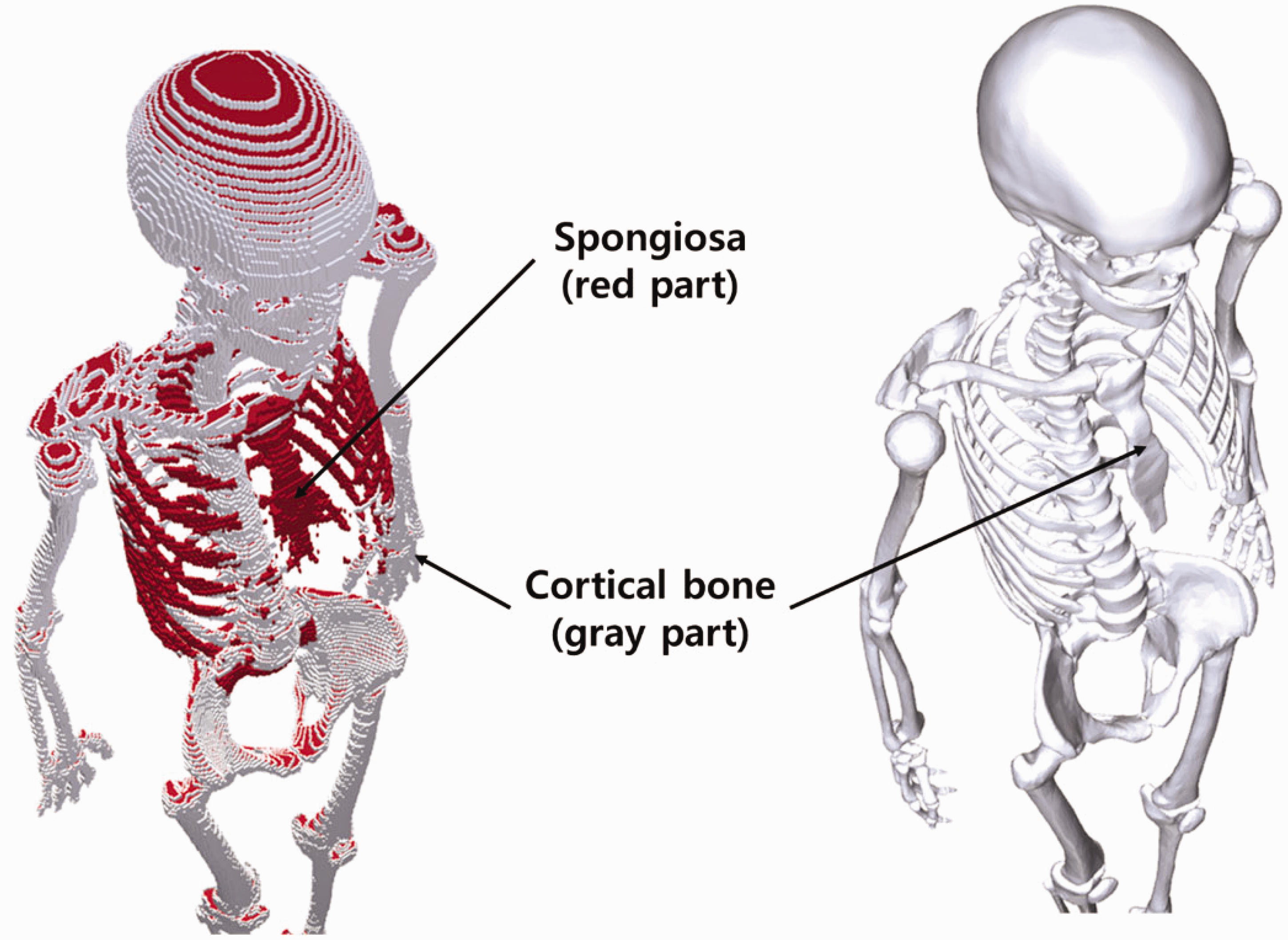
(72) Figs 6.1 and 6.2 show the adult male and female MRCPs, respectively. The height and weight of the MRCPs are in accordance with the reference values (male 176 cm and 73 kg, female 163 cm and 60 kg). The male phantom is composed of 2.5 million triangular facets in the PM format and 8.2 million tetrahedrons in the TM format. The female phantom is composed of 2.6 million triangular facets in the PM format and 8.6 million tetrahedrons in the TM format. Note that the TM MRCPs were converted directly from the PM MRCPs using the TetGen code (Si, 2015). The MRCPs include all the radiosensitive organs and tissues relevant to dose assessment for ionising radiation exposure for radiological protection purposes. Note that the micron-scale structures of the active bone marrow and skeletal endosteum are not modelled in the MRCPs and, therefore, the calculation of the doses to these skeletal tissues should involve fluence-to-dose–response functions, such as those presented in Publication 116 (ICRP, 2010). The MRCPs include the tens-of-micrometre-thick source and target regions of the lens of the eye, skin, alimentary tract organs, respiratory tract organs, and urinary bladder. The lung airway models (representing the various branches of both the bronchi and bronchioles) produced in the CSG format are incorporated into the MRCPs using the Geant4 code (Agostinelli et al., 2003) via the parallel-geometry technique (Apostolakis et al., 2008). (73) The masses of the organs and tissues of the MRCPs match the reference values inclusive of blood content (see Table 4.2) within 0.1% deviation. Table A.1 provides the numerical information of the MRCPs including the organ ID number, medium, density, and mass for each organ and tissue. Tables B.1 and B.2 provide the elemental composition for each medium for the male and female, respectively. Table C.1 provides the list of source regions, their acronyms, and corresponding organ ID numbers in the phantoms. Table D.1 provides the list of target regions, their acronyms, and corresponding organ ID numbers in the phantoms. (74) For the alimentary and respiratory tract organs, the dose values of the thin target regions, due to the tiny volumes, tend to have larger statistical uncertainties compared with other organs. For external exposures to penetrating radiation (such as photons and neutrons), the spatial gradients of the absorbed dose are very small, and thus the absorbed dose averaged over the thin target region tends to be close to the absorbed dose averaged over the entire region of the organ. Therefore, for these exposure cases, it is recommended that one use the entire region of the organ, not the thin target region, for dose calculation in order to save computation time. (75) On the other hand, the target region of the skin and lens of the eye should be used in dose calculation for all external exposure cases, considering that there will be significant dose differences between the target region and the entire region even for penetrating uncharged particles (such as photons and neutrons), because charged-particle equilibrium is not well established in these superficial organs. For the skin dose calculation, computation time is no longer a problem assuming the entire skin is exposed to the incident radiation field. For the lens dose calculation, computation time can be reduced significantly by assuming that only the head of the phantoms is exposed to radiation. (76) The thin target regions of the alimentary and respiratory tract systems and the urinary bladder should be used in dose calculation for internal exposure cases when subregions of these organs (e.g. contents) are considered as source regions. For these calculations, computation time is no longer an issue considering the layered geometries of the source and target regions. (77) For cross-fire irradiation (e.g. stomach ← liver), it is recommended that one use the entire region of the organ, not just the thin target region, for dose calculation, as once again, dose gradients are small and there will be a saving in computation time. For electron cross-fire irradiation, there could be significant dose discrepancies, depending on the electron energy and organ topology, in which case it is recommended to use the thin target region. (78) The MRCPs have addressed the geometric limitations of the Publication 110 (ICRP, 2009) phantoms due to the limited voxel resolution and the nature of voxel geometry. Fig. 6.3 shows some internal organs and tissues of the male MRCP alongside those of the Publication 110 male phantom. It can be seen that the voxel models show stair-stepped surfaces, whereas the mesh models show smooth surfaces in their 3D viewing. In addition, the discontinuous structure of the hollow organs of the Publication 110 phantoms is fully addressed in the MRCPs. Fig. 6.4 shows the female MRCP and the Publication 110 female phantom viewed in the superior–inferior direction. It can be seen that the Publication 110 phantoms are not fully enclosed by the skin, showing many holes and several radiosensitive organs and tissues (such as breasts and muscle) directly exposed to the air. On the other hand, the MRCPs are fully enclosed by the skin without any holes; this improvement will prevent significant overestimates in DCs for these organs and tissues for specific situations of external exposure to weakly-penetrating radiation. Similarly, the spongiosa and medullary cavity of the Publication 110 phantoms are not fully enclosed by the cortical bone; this limitation is also addressed in the MRCPs, as shown in Fig. 6.5. Mesh-type ICRP adult male reference phantom. Mesh-type ICRP adult female reference phantom. Comparison of organs and tissues of the mesh-type male phantom with those of the Publication 110 (ICRP, 2009) male phantom. Publication 110 (ICRP, 2009) female phantom (left) and mesh-type female phantom (right): muscle (blue green part), spongiosa (red part), and breasts (yellow part) in Publication 110 female phantom. Skeletal system of Publication 110 (ICRP, 2009) female phantom (left) and mesh-type female phantom (right): spongiosa (red part) and cortical bone (gray part). The mesh phantom only shows cortical bone (gray part) which fully encloses inner structures (spongiosa and medullary cavity).
6.2. Geometric similarity comparison with the adult voxel-type reference phantoms
(79) In order to determine the geometric similarity between the MRCPs and the adult voxel-type reference phantoms, DI, CD, and HD values for the organs and tissues between these phantoms were evaluated as shown in Table 6.1. It can be seen that for most organs and tissues, DI values were >0.8, and CD and HD values were <2 mm. These results demonstrate good geometric similarity between the MRCPs and the Publication 110 (ICRP, 2009) phantoms in general. (80) There were, however, relatively large dissimilarities for some organs and tissues. For example, the female hand bone showed the greatest dissimilarity; DI, CD, and HD values were 0.13, 27.8 mm, and 15.6 mm, respectively. Such large dissimilarities are mainly due to two reasons: (1) organs and tissues such as spine, hands, feet, and small intestine could not be converted directly from the voxel models, and therefore were constructed with modelling approaches; and (2) organs and tissues such as ribs, liver, spleen, and kidneys were adjusted more significantly to include blood content, despite the fact that these organs were mainly constructed using the direct conversion method. (81) The ODDs and CLDs of the MRCPs were also compared with those of the Publication 110 (ICRP, 2009) phantoms, as shown in Annexes E and F. The ODDs represent the organ depth below the body surface, which mainly influences external dose calculation, and the CLDs represent the distance between the target and source organs/tissues, which mainly influences internal dose calculation. The comparison results showed that the ODDs and CLDs of the MRCPs were generally in good agreement with those of the Publication 110 phantoms for most organs and tissues, despite the fact that the MRCPs were adjusted for the inclusion of blood content. (82) The results of the geometric similarity comparison indicate that, overall, the MRCPs faithfully preserve the original shape and location of the organs and tissues in the Publication 110 (ICRP, 2009) phantoms, and that, therefore, they can be expected to provide similar dose values for penetrating radiation in both external and internal exposures. Dice index (DI), centroid distance (CD), and Hausdorff distance (HD) comparing the adult MRCPs and the adult voxel-type reference phantoms.

6.3. Compatibility with Monte Carlo codes
6.3.1. Monte Carlo codes
(83) Most of the major general-purpose Monte Carlo simulation codes such as Geant4, MCNP6, PHITS, and FLUKA can now implement PM or TM geometries directly. The Geant4 code implements both PM and TM geometries using the G4TessellatedSolid class and G4Tet class, respectively (Agostinelli et al., 2003). The MCNP6 code, as a merger of the MCNP5 and MCNPX versions, provides a new feature for implementation of unstructured mesh geometries, including TM geometries. Note that since Version 1.1 beta of the MCNP6 code, the unstructured mesh geometry can support the transport of most particles available in the MCNP6 code (Goorley et al., 2013), whereas in the previous version (i.e. Version 1.0), only the transport of neutrons and gamma rays was supported (Martz, 2014). The PHITS code, since Version 2.82, provides a new feature for implementation of TM geometries (Sato et al., 2013). The FLUKA code can implement the PM geometry via FluDAG (http://svalinn.github.io/DAGMC/index.html).
6.3.2. Computation time and memory usage
(84) Computation time was measured for the Geant4 (Version 10.02), MCNP6 (Version 2.0), and PHITS (Version 2.92) codes coupled with the female phantom of the TM format. The estimation was performed on a single core of the Intel Xeon CPU X5660 (2.80 GHz and 128 GB memory). First, the estimated initialisation times for all Monte Carlo codes were found to be a few minutes, which is negligible compared with the total computation time on the order of a day which is a typical value for dose calculations (Furuta el al., 2017). (85) Run time was also measured with a single core of the same server computer to achieve 2% of relative error in effective dose for the left lateral irradiation geometry of particle beams: photons and electrons (10 keV–10 GeV) and neutrons (10−9 MeV–20 MeV). For the Geant4 code, the physics library of G4EmLivermorePhysics was used to transport photons and electrons. To transport neutrons, the physics models and cross-sections of NeutronHPThermalScattering, NeutronHPElastic, ParticleHPInelastic, Neutron-HPCapture, and NeutronHPFission were used. A secondary cut value of 1 µm was applied to photons and electrons. For the PHITS code, the physics library of AcelibJ40 was used to transport photons, electrons, and neutrons. For the MCNP6 code, the physics libraries of MCPLIB84, EL03, and ENDF70 were used to transport photons, electrons, and neutrons, respectively. Considering that a secondary cut value of 1 µm was used for the Geant4 calculations, the equivalent energy cut values were used in the PHITS and MCNP6 codes. The ‘implicit capture’ variance reduction technique was turned off for both the PHITS and MCNP6 codes. (86) The Geant4 result showed that for photons, the measured run times were within the range of 1–30 min for all of the considered energies. For electrons, the run times were <1 h for energies >0.06 MeV, but for lower energies (≤0.06), the run times were much longer (i.e. 20–60 h). These long run times are due to the fact that these low-energy electrons cannot penetrate the dead layer of skin, and that only the secondary photons, produced from electron interactions, contribute to skin dose and, eventually, effective dose. For neutrons, the run times were within the range of 2–30 h for all of the considered energies. (87) The run times of the PHITS code for photons and electrons were generally much longer (i.e. three to 20 times longer) compared with the Geant4 code. Similarly, the run times of the MCNP6 code were longer (i.e. six to 30 times longer) than those of the Geant4 code. For neutrons, the run times of the PHITS code were two to eight times shorter than those of the Geant4 code, whereas those of the MCNP6 code were three to four times longer than those of the Geant4 code. (88) Memory usage was also measured for the three Monte Carlo codes. The Geant4 code required ∼10.6 GB, which is slightly less than that of the MCNP6 code (∼13.7 GB). The PHITS code, when compared with the Geant4 and MCNP6 codes, required much less memory (i.e. ∼1.2 GB) due to the fact that the PHITS code, in contrast to other codes, uses dynamic allocation for most of the memory needed for implementing the MRCPs. In general, considering memory usage, all of the above Monte Carlo codes can run the MRCPs in a personal computer equipped with 64 GB at maximum.
7. DOSIMETRIC IMPACT Of THE ADULT MESH-TYPE REFERENCE PHANTOMS
(89) In order to investigate the impact of the improved representation of organs and tissues in the adult MRCPs on DC calculations, DCs of organ dose and effective dose and SAFs were calculated for some selected external and internal exposure cases using the MRCPs. The calculated values were then compared with the values provided in Publications 116 and 133 (ICRP, 2010, 2016), which were calculated using the Publication 110 (ICRP, 2009) phantoms and the stylised models adopted in the previous Publications (ICRP, 1994a, 2006, 2016). (90) In Annex H, the DCs of the MRCPs for external exposure to photons, neutrons, electrons, and helium ions are compared with the Publication 116 (ICRP, 2010) values. For photons, with some exceptions at very low energies, the DCs of the MRCPs were found to be very close to the Publication 116 values for both organ dose and effective dose. For neutrons, the organ DCs of the MRCPs show some differences from the Publication 116 values, but are very close to the values calculated using the Publication 110 (ICRP, 2009) phantoms and the Geant4 code that was the same code used in calculation of the MRCP DCs. This result indicates that the differences from the Publication 116 values are not mainly due to the difference in phantom geometry or material composition, but due to the difference in Monte Carlo codes and cross-section data/physics models used in the calculations. Note that for neutrons, the Publication 116 values were calculated using four Monte Carlo codes (MCNPX, PHITS, FLUKA, and Geant4) and then the final reference values of the DCs were taken as averaged values following an extensive smoothing process (ICRP, 2010). (91) In Annex H, for charged particles (i.e. electrons and alpha particles), the DCs of the MRCPs for some organs (e.g. RBM, breasts, and skin) showed large differences from the Publication 116 (ICRP, 2010) values, mainly due to improved representation of the thin tissues (e.g. cortical bone and skin) in the MRCPs over the voxel-type Publication 110 (ICRP, 2009) phantoms (see Section 2). Large differences were also found in effective dose DCs for electrons (<1 MeV) and helium ions (<10 MeV u−1); these differences are mainly caused by differences in skin DCs due to consideration of the 50-µm-thick skin target layer in the MRCPs. Note that in real situations of electron exposure, polyenergetic electrons are generally encountered, for which the differences in effective doses are much less significant. For example, the differences in effective dose between the MRCPs and the Publication 110 phantoms resulting from the isotropic irradiation of beta radiations (14C, 186Re, 32P, 90Sr/90Y, and 106Rh) are less than two-fold, except for 14C for which the difference is approximately four-fold. Note that 14C emits very-low-energy electrons (0.15 MeV maximum) and thus is generally not of concern for external exposures. In real situations of helium ion exposure, short-range alpha exposures are mainly encountered, which are practically unimportant for radiation protection purposes. (92) In Annex I, the SAFs of the MRCPs for photons and electrons are compared with the Publication 133 (ICRP, 2016) values for selected source organs/tissues (cortical bone, liver, lungs, and thyroid). For photons, with some exceptions, the SAFs of the MRCPs were found to be very close to the Publication 133 values. One exception was the RBM as a target, where the SAFs of the MRCPs were much smaller than the Publication 133 values at low energies. These differences are mainly due to the fact that in the MRCPs, the spongiosa is fully enclosed by the cortical bone, whereas this is not the case for the Publication 110 (ICRP, 2009) phantoms (see Fig. 6.5). In contrast, for the colon ← cortical bone case, the SAFs of the MRCPs were found to be greater than the Publication 133 values, mainly due to the difference in distribution of the cortical bone; that is, in the Publication 110 phantoms, the cortical bone does not fully enclose the spongiosa and is not distributed uniformly, especially in the ribs where the cortical bone is rarely distributed in the regions that are very close to the colon. (93) In Annex I, for electrons, the SAFs of the MRCPs were found to be very close to the Publication 133 (ICRP, 2016) values for all of the self-irradiation cases. However, large differences were found for most cross-fire irradiation cases, mainly due to the different geometric formats of the phantoms [smooth surface of the MRCPs vs stair-stepped surface of the Publication 110 (ICRP, 2009) phantoms]. The significance of these differences on effective dose will be dependent on the biokinetics or chemical form of ingested or inhaled radionuclide. (94) In Nguyen et al. (2015), the lens DCs of the MRCPs for external exposure to photons and electrons were compared with the Publication 116 (ICRP, 2010) values that were produced with both the Publication 110 (ICRP, 2009) voxel phantoms and the mathematical eye model of Behrens et al. (2009). The comparison was complicated because different phantoms were used for different cases in Publication 116. For photons, the lens DCs of the MRCPs were similar to the Publication 116 values for all of the irradiation geometries, except for the posterior–anterior geometry and low energies (<0.1 MeV), in which cases the lens DCs of the MRCPs were smaller than the Publication 116 values. These differences are not very important in practice, and are mainly due to differences in head structure and composition between the MRCPs and the mathematical head phantom (incorporating the eye model) used to produce the Publication 116 values. For electrons, the lens DCs of the MRCPs were generally found to be very close to the Publication 116 values at energies ≥2 MeV, but at the lower energies (<2 MeV), relatively large differences were found. The largest differences were found in the posterior–anterior geometry due to differences in head structure and composition between the MRCPs and the Publication 110 phantoms used to produce the Publication 116 values. For the anterior–posterior irradiation geometry, which is the most important irradiation geometry in radiation protection, the differences were much smaller, and significant differences were only observed at very low energies (<0.7 MeV) where primary electrons cannot reach the lens and thus very-low-energy secondary photons are the only contribution to lens dose. More detailed discussions on comparison of lens DCs can be found in Nguyen et al. (2015). (95) In Kim et al. (2017), the electron SAFs of the MRCPs for the alimentary and respiratory tract systems were compared with the Publication 133 (ICRP, 2016) values that were calculated using the supplementary stylised models (ICRP, 1994a, 2006, 2016). Generally, good agreement was observed for the oral mucosa, oesophagus, and BB region. In contrast, for the stomach, small intestine, large intestine, ET region, and bb region, relatively large differences were observed, mainly due to anatomical differences of these organs as described by the MRCPs and the stylised models. With some exceptions (stomach and bb region for the AI region as a source), the MRCPs tend to overestimate SAFs when compared with the Publication 133 values; the maximum difference was approximately 16 times for the large intestine for the contents as a source. To use the MRCPs for SAF calculations, one should be aware that the masses of the target regions (i.e. stem cells) for the stomach and intestines in the MRCPs do not exactly match those of the stylised models in Publication 100 (ICRP, 2006). (96) The electron cross-fires between respiratory tract segments in the lungs are naturally realised in the MRCPs, which is one of the main advantages of using the MRCPs over the isolated cylindrical stylised models in Publication 66 (1994a). Fig. 7.1 shows, as an example, the SAF results for the secretory cells of the bronchioles (bbsec) as a target. Except for the AI source region where significant SAF differences were found due to the different AI densities, it can be seen that an overall trend is similar for all source regions. For energies <0.5 MeV, the SAFs of the MRCPs show good agreement with those of the stylised models; that is, the maximum differences were only 14% and 18% for the male and female, respectively. For higher energies, on the other hand, significant differences can be found; that is, the MRCPs produce higher SAFs than the stylised models, by up to 77% and 74% for the male and female, respectively, mainly due to realisation of the cross-fires in the MRCPs. More detailed discussions on comparison of the SAFs for the alimentary and respiratory tract systems can be found in Kim et al. (2017). (97) The male MRCP was used to calculate the SAFs for alpha particles and electrons for the urinary bladder wall ← urinary bladder content case, and then the calculated values were compared with the values calculated using a stylised model for the male (Eckerman and Veinot, 2018). Note that the values of the MRCP were not compared with the values in Publication 133 (ICRP, 2016) because these values were calculated for the entire wall of the urinary bladder, not for the radiosensitive basal layer of the wall. The MRCP values were found to be slightly less than the values of the stylised model, the differences being less than a few percent, mainly due to the slight difference (∼6%) in the target mass between the MRCP urinary bladder model and the idealised spherical stylised model used in Eckerman and Veniot (2018). Specific absorbed fractions to the secretory cells of the bronchioles (bbsec) as a target for electron exposures within the male mesh-type reference computational phantom (MRCP) (red circles), female MRCP (red squares), Publication 66 (ICRP, 1994a) stylised male model (blue upward triangles), Publication 66 stylised female model (blue downward triangles), Publication 133 (ICRP, 2016) male values (black solid line), and Publication 133 female values (black dashed line) (Kim et al., 2017).
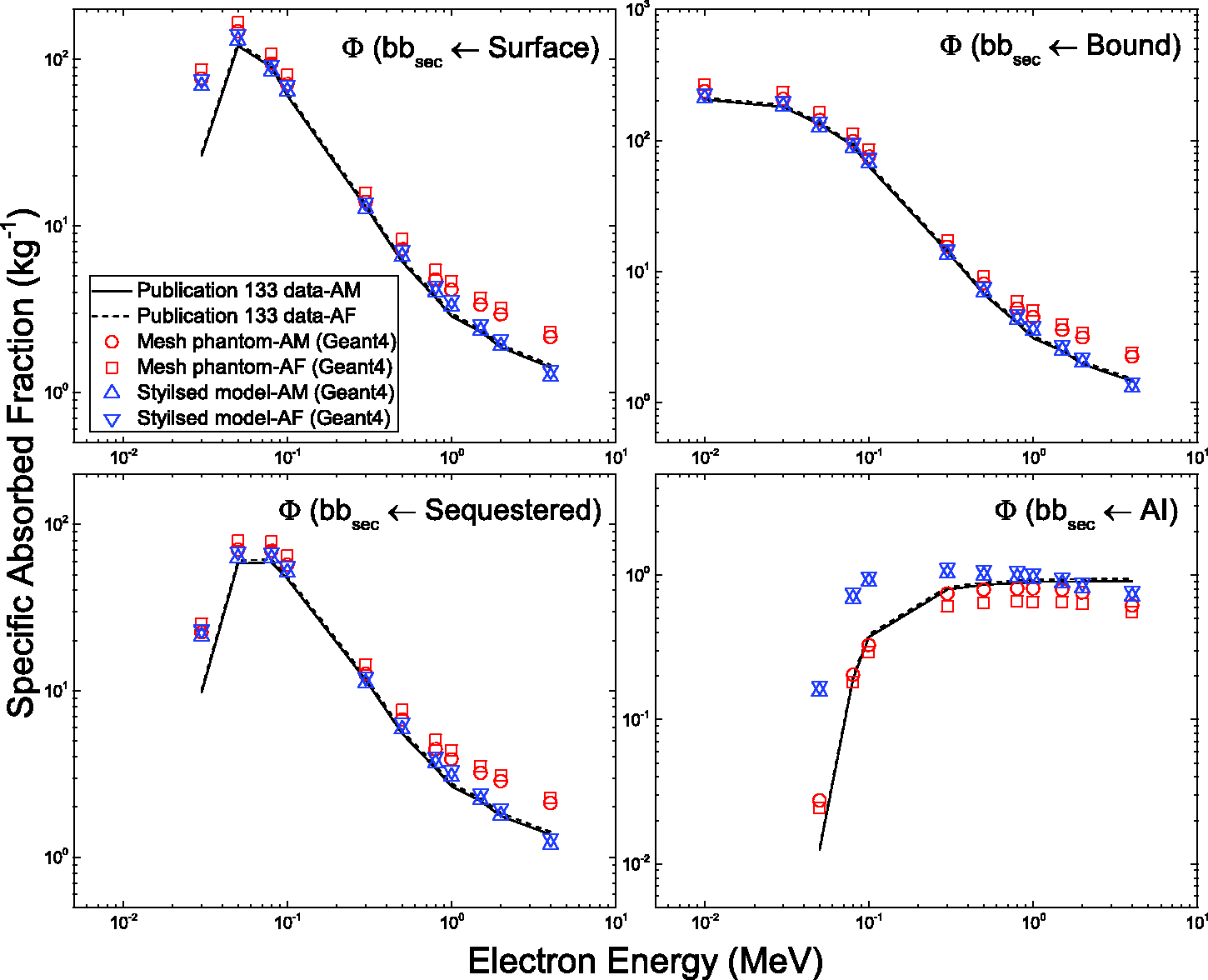
8. APPLICATION: CALCULATION OF DOSE COEFFICIENTS FOR INDUSTRIAL RADIOGRAPHY SOURCES
(98) Accidents involving industrial radiography sources could result in very high radiation doses to workers, causing serious injuries and even death (IAEA, 2011). In addition, members of the public could be exposed accidentally if industrial radiography sources are not properly controlled or regulated. According to the International Atomic Energy Agency (IAEA, 1998), industrial radiography accounts for approximately half of all reported accidents for nuclear-related industries in both developed and developing countries. Radiation accidents could result in high radiation doses inducing acute radiation syndrome (ARS), which can be classified into haematopoietic (3–5 Gy), gastrointestinal (5–15 Gy), and cerebrovascular (>15 Gy) syndromes (ICRP, 2007). In order to treat patients (i.e. exposed individuals) with ARS effectively, it is necessary to perform medical triage accurately and quickly, whereby those patients who will develop symptoms are identified separately from those who do not require medical intervention (Gougelet et al., 2010). Individual radiation doses can be estimated using various dosimetric techniques based on biological, physical, or computational approaches. However, all of the existing dosimetric techniques have limitations, and thus none of them can be used as a stand-alone tool in a satisfactory manner for most radiation accident scenarios (Ainsbury et al., 2011). For example, biological and physical dosimetric techniques generally require several days for sample collection and analysis. Moreover, these techniques are impractical for use in a large-scale accident involving a multitude of exposed individuals (Gougelet et al., 2010; Rea et al., 2010; Swartz et al., 2014; Kulka et al., 2017), and are generally limited to estimating the whole-body dose without information on organ-/tissue-specific doses or their dose distribution (Ainsbury et al., 2011). Note that knowledge of the whole-body dose may not be sufficient, especially in partial-body or localised exposures (Ainsbury et al., 2011; Lu et al., 2017). Organ/tissue doses or dose distributions can be estimated using computational dosimetric techniques (e.g. Monte Carlo simulations with computational human phantoms) if reliable information on the accident scenario is available, including the source geometry and duration of exposure (Lu et al., 2017), which are often unclear immediately following accidental irradiation situations (Clairand et al., 2006; Ainsbury et al., 2011). Due to the fact that no single technique fully meets the criteria of an ideal dosimeter for use in accidental situations, an integrated approach using multiple dosimetric techniques is considered to be the best strategy (Ainsbury et al., 2011, 2017; Sullivan et al., 2013). Doses calculated with computational anthropomorphic phantoms can be used as one of the dose estimators, particularly as an ‘initial, rapid estimator’. (99) For dose estimation of individuals exposed to such high doses, consideration of the Reference Person may be insufficient, particularly when the body size of the individual involved in the accident is significantly different from that of the phantom representing the Reference Person. In such cases, the dose could be better approximated using DCs calculated with a non-reference computational phantom whose body size is close to that of the actual person. To demonstrate this approach, non-reference adult male and female phantoms, representing the 10th and 90th percentiles of the Caucasian population, were developed in this publication. The 10th percentile phantoms, which represent small people, were constructed by decreasing the size of the MRCPs to the 10th percentile standing height and the 10th percentile body mass (male 1.672 m and 55.9 kg, female 1.549 m and 44.2 kg). Similarly, the 90th percentile phantoms, which represent large people, were constructed by increasing the size of the MRCPs to the 90th percentile standing height and the 90th percentile body mass (male 1.858 m and 108.4 kg, female 1.717 m and 94.1 kg). Fig. 8.1 shows the 10th and 90th percentile phantoms, along with the MRCPs. The height and mass values were derived from PeopleSize 2008 Professional data (http://www.openerg.com). The torso, arms, and legs were scaled considering the lean body mass (Deurenberg et al., 1991; Pieterman et al., 2002). The head was scaled separately, using PeopleSize 2008 Professional data and the US Army Anthropometric Survey (ANSUR II) data (Gordon et al., 2014). More detailed information on scaling can be found in Lee et al. (2019). The internal organs and tissues of the phantoms were modified via the scaling/deforming procedures as described in Lee et al. (2019). (100) In order to evaluate accidental exposures from industrial radiography sources, DCs were calculated using the adult MRCPs as well as the 10th and 90th percentile phantoms, implemented into the Geant4 code (Version 10.02) (Agostinelli et al., 2003). The most commonly used industrial radiography sources (i.e. 192Ir, 137Cs/137mBa, and 60Co) were simulated as point sources placed near each of the MCRPs. 192Ir emits gamma rays with energies up to 0.820 MeV and a mean energy of 0.377 MeV, 137Cs emits 0.662 MeV gamma rays, and 60Co emits 1.33 and 1.17 MeV gamma rays. The point sources were assumed to be located at three different distances (0.005, 0.1, and 0.3 m) in four directions (anterior, posterior, right lateral, and left lateral) at five levels (ground, middle thigh, lower torso, middle torso, and upper torso) (see Fig. 8.2). In addition, three longer distances (1, 1.5, and 3 m) were modelled in the four directions at the lower torso level. The source distance used in the calculations is the distance from the surface of the phantom, except for the anterior and posterior directions at ground and middle thigh levels, for which the distance is calculated from the centre of the imaginary segment tangent to the surfaces of the left and right legs at the given level. (101) In order to consider the doses of those organs/tissues that might manifest ARS, the doses for RBM, brain, lungs, small intestine, and large intestine were calculated as organ-/tissue-averaged absorbed dose per source disintegration (Gy s−1 Bq−1). The RBM DCs were calculated using the fluence-to-absorbed-dose-response functions reported in Annex D of Publication 116 (ICRP, 2010). In addition, the DCs of effective dose (effective dose per source disintegration) were calculated and could be used for the dosimetry of individuals who are exposed at lower doses related to stochastic effects. Effective doses cannot be calculated using non-reference phantoms (i.e. 10th and 90th percentile phantoms) and, therefore, in this publication, the DCs of effective doses were only calculated using the MRCPs. The statistical errors of the calculated values were <5% for all cases. A complete set of the DCs calculated with the MRCPs and the 10th and 90th percentile phantoms is given in Annex J. (102) Furthermore, the influence of different postures during exposure was investigated by calculating DCs using a set of non-standing phantoms (walking, sitting, bending, kneeling, and squatting postures) that were constructed by modifying the MRCPs. For this purpose, the DCs were calculated for the lowest-energy source (i.e. 192Ir) located 1 m from the phantom surface in the four directions at lower torso level. The calculated DCs of the non-standing phantoms were then compared with those of the standing MRCPs. The results of this limited investigation showed that the influence of different postures on the DC is not very large (generally <30%). It was, therefore, decided not to calculate the DCs of the non-standing phantoms. (103) Note that the strength of industrial radiography sources is usually given as ‘apparent activity’ (also called ‘effective activity’), which is defined as the activity of an unshielded point source that would give the same exposure rate at the same distance (typically 1 m) compared with the actual source (Gomes et al., 2013). If the source strength is given as real physical activity, not apparent activity, the DCs listed in Annex J should be corrected to take the source self-shielding effect into account. Therefore, Annex J also provides the source self-shielding factors for different thicknesses of radioactive material and capsule wall. Computational phantoms for adult male (top) and adult female (bottom): 10th percentile phantom (left), mesh-type reference computational phantom (middle), and 90th percentile phantom (right). Source locations at three distances (0.005, 0.1, and 0.3 m) at five levels (ground, middle thigh, lower torso, middle torso, and upper torso) in four directions (anterior, posterior, right lateral, and left lateral).
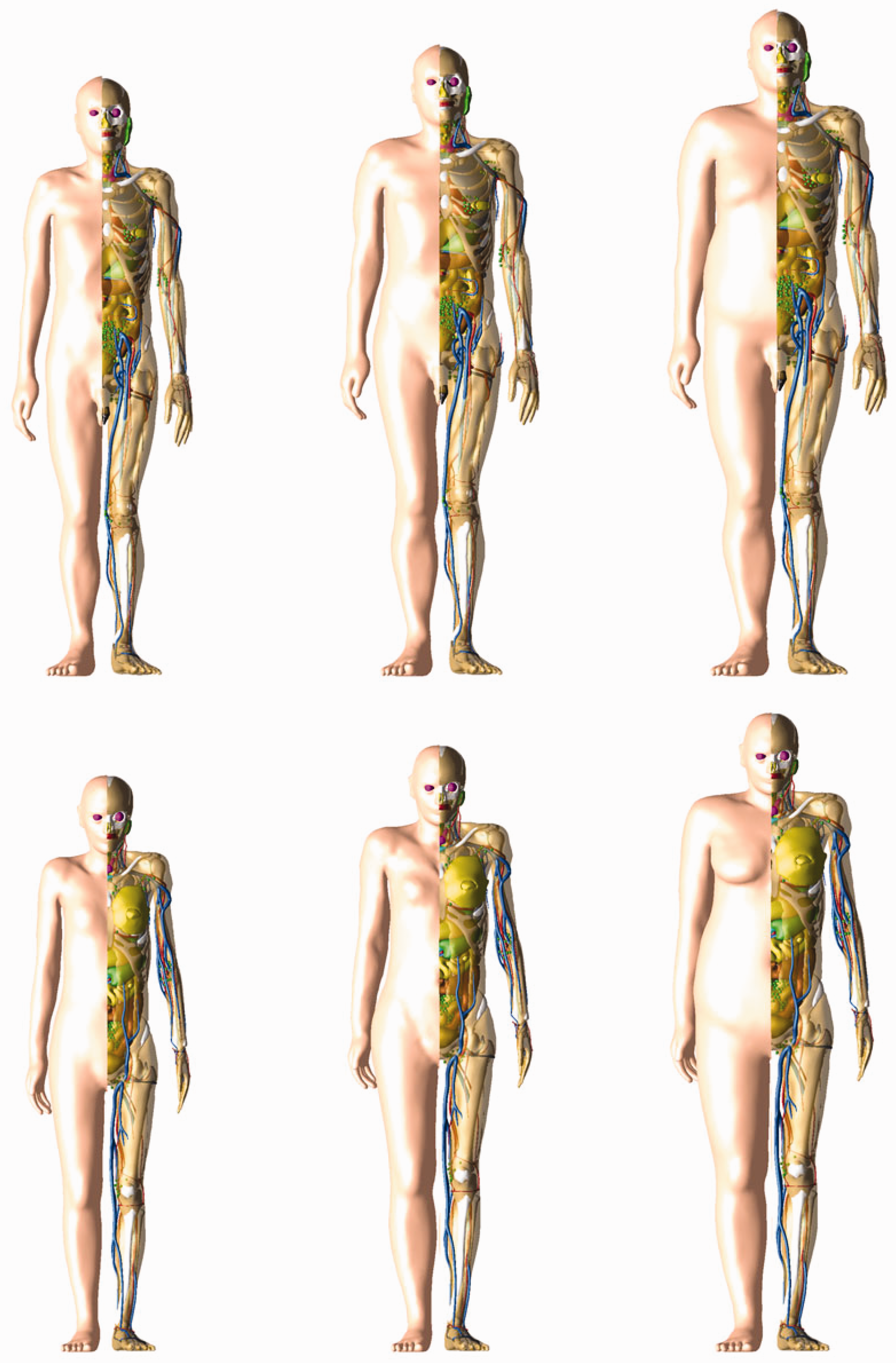
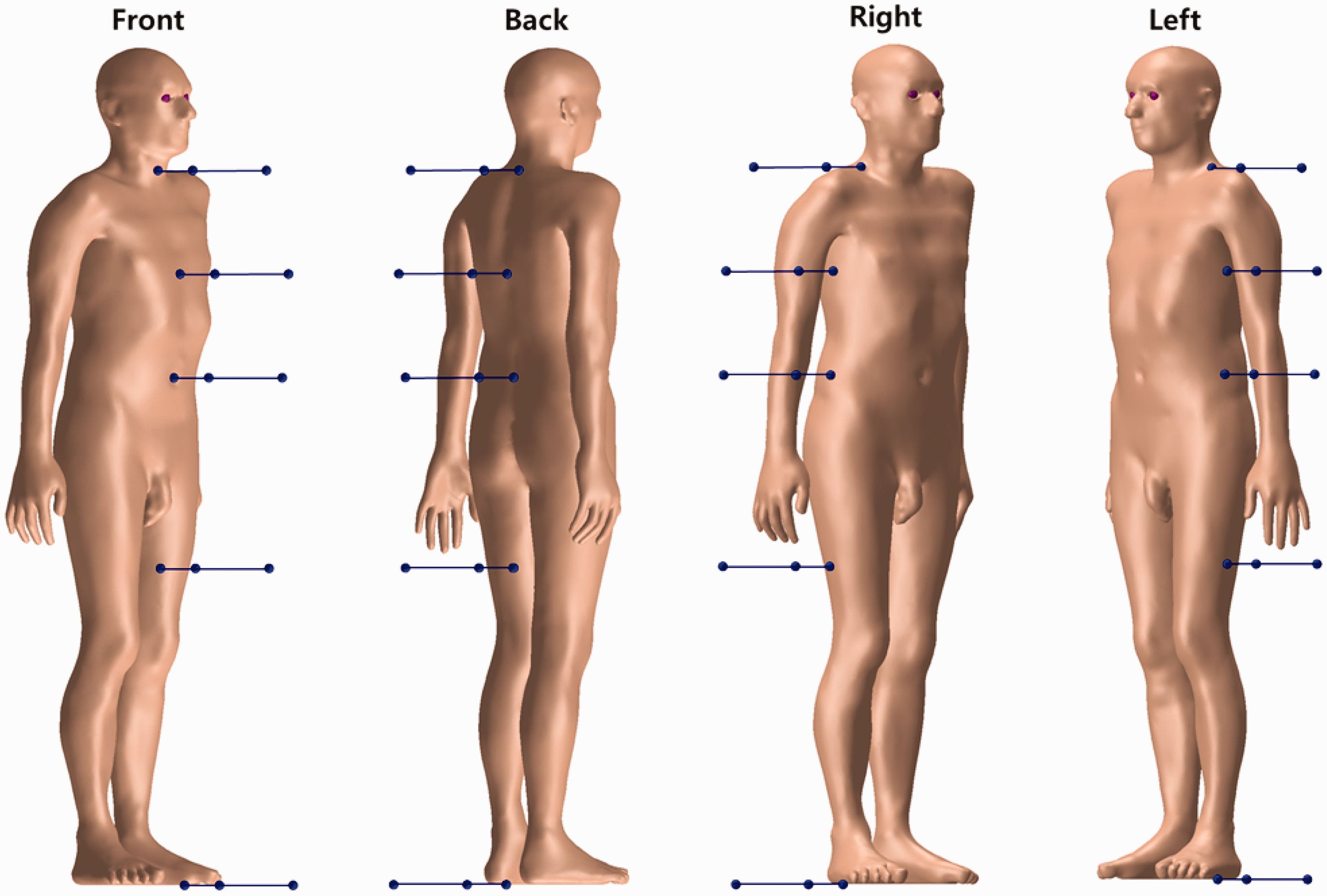
Supplemental Material
sj-zip-1-ani-10.1177_0146645319893605 - Supplemental material for ICRP Publication 145: Adult Mesh-Type Reference Computational Phantoms
Supplemental material, sj-zip-1-ani-10.1177_0146645319893605 for ICRP Publication 145: Adult Mesh-Type Reference Computational Phantoms by C.H. Kim, Y.S. Yeom, N. Petoussi-Henss, M. Zankl, W.E. Bolch, C. Lee, C. Choi, T.T. Nguyen, K. Eckerman, H.S. Kim, M.C. Han, R. Qiu, B.S. Chung, H. Han and B. Shin in Annals of the ICRP
Footnotes
ANNEX A. LIST OF ORGAN identification numbers,MEDIUM,DENSITY,AND MASS OF EACH ORGAN/TISSUE
List of organ identification (ID) number, medium, density, and mass of each organ/tissue in polygon mesh (PM) phantoms.
| Organ ID | Organ/tissue | Medium | Density (g cm−3) |
Mass (g) |
||
|---|---|---|---|---|---|---|
| Male | Female | Male | Female | |||
| 100 | Adrenal, left | 1 | 1.036 | 1.035 | 8.683 | 6.817 |
| 200 | Adrenal, right | 1 | 1.036 | 1.035 | 8.683 | 8.649 |
| 300 | ET1, 8 µm | 2 | 1.031 | 1.031 | 0.022 | 0.009 |
| 301 | ET1, 40 µm | 2 | 1.031 | 1.031 | 0.090 | 0.035 |
| 302 | ET1, 50 µm | 2 | 1.031 | 1.031 | 0.028 | 0.011 |
| 303 | ET1, surface | 2 | 1.031 | 1.031 | 11.291 | 4.375 |
| 400 | ET2, 0 µm | 52 | 1.000 | 1.000 | 0.141 | 0.104 |
| 401 | ET2, 40 µm | 2 | 1.031 | 1.031 | 0.390 | 0.288 |
| 402 | ET2, 50 µm | 2 | 1.031 | 1.031 | 0.098 | 0.072 |
| 403 | ET2, 55 µm | 2 | 1.031 | 1.031 | 0.049 | 0.036 |
| 404 | ET2, 65 µm | 2 | 1.031 | 1.031 | 0.098 | 0.072 |
| 405 | ET2, surface | 2 | 1.031 | 1.031 | 28.808 | 14.180 |
| 500 | Oral mucosa, tongue | 3 | 1.050 | 1.050 | 0.086 | 0.066 |
| 501 | Oral mucosa, mouth floor | 3 | 1.050 | 1.050 | 0.023 | 0.016 |
| 600 | Oral mucosa, lips and cheeks | 3 | 1.050 | 1.050 | 0.023 | 0.019 |
| 700 | Trachea | 2 | 1.031 | 1.031 | 10.364 | 8.201 |
| 800 | BB1 * , −6 µm | 52 | 1.000 | 1.000 | 0.025 | 0.010 |
| 801 | BB1 * , 0 µm | 2 | 1.031 | 1.031 | 0.031 | 0.013 |
| 802 | BB1 * , 10 µm | 2 | 1.031 | 1.031 | 0.052 | 0.021 |
| 803 | BB1 * , 35 µm | 2 | 1.031 | 1.031 | 0.130 | 0.053 |
| 804 | BB1 * , 40 µm | 2 | 1.031 | 1.031 | 0.026 | 0.011 |
| 805 | BB1 * , 50 µm | 2 | 1.031 | 1.031 | 0.052 | 0.021 |
| 806 | BB1 * , 60 µm | 2 | 1.031 | 1.031 | 0.052 | 0.021 |
| 807 | BB1 * , 70 µm | 2 | 1.031 | 1.031 | 0.053 | 0.021 |
| 808 | BB1 * , surface | 2 | 1.031 | 1.031 | 2.777 | 1.179 |
| 900 | Blood in large arteries | 4 | 1.060 | 1.060 | 336.000 | 246.000 |
| 910 | Blood in large veins | 4 | 1.060 | 1.060 | 1008.000 | 737.998 |
| 1300 | Humeri, cortical | 5 | 1.904 | 1.904 | 265.917 | 216.977 |
| 1400 | Humeri, upper, spongiosa | 7 | 1.233 | 1.185 | 145.689 | 107.717 |
| 1500 | Humeri, medullary cavity | 6 | 0.981 | 0.981 | 71.641 | 41.009 |
| 1700 | Humeri, lower, spongiosa | 8 | 1.109 | 1.117 | 50.890 | 50.264 |
| 1900 | Ulnae and radii, cortical | 5 | 1.904 | 1.904 | 273.498 | 156.708 |
| 2000 | Ulnae and radii, spongiosa | 8 | 1.109 | 1.117 | 154.981 | 86.883 |
| 2100 | Ulnae and radii, medullary cavity | 6 | 0.981 | 0.981 | 22.996 | 34.068 |
| 2200 | Wrists and hand bones, cortical | 5 | 1.904 | 1.904 | 181.529 | 105.132 |
| 2300 | Wrists and hand bones, spongiosa | 8 | 1.109 | 1.117 | 118.927 | 69.360 |
| 2400 | Clavicles, cortical | 5 | 1.904 | 1.904 | 48.252 | 32.825 |
| 2500 | Clavicles, spongiosa | 9 | 1.157 | 1.192 | 45.057 | 38.798 |
| 2600 | Cranium, cortical | 5 | 1.904 | 1.904 | 567.517 | 405.466 |
| 2600 | Cranium, cortical, surrounding frontal sinus | 5 | 1.904 | 1.904 | 0.953 | 2.204 |
| 2700 | Cranium, spongiosa | 10 | 1.165 | 1.252 | 382.073 | 391.311 |
| 2800 | Femora, cortical | 5 | 1.904 | 1.904 | 561.309 | 485.055 |
| 2900 | Femora, upper, spongiosa | 11 | 1.125 | 1.046 | 413.232 | 232.804 |
| 3000 | Femora, medullary cavity | 6 | 0.981 | 0.981 | 108.224 | 96.278 |
| 3200 | Femora, lower, spongiosa | 8 | 1.109 | 1.117 | 373.652 | 166.334 |
| 3400 | Tibiae, fibulae, and patellae, cortical | 5 | 1.904 | 1.904 | 536.651 | 544.845 |
| 3500 | Tibiae, fibulae, and patellae, spongiosa | 8 | 1.109 | 1.117 | 621.408 | 558.529 |
| 3600 | Tibiae, fibulae, and patellae, medullary cavity | 6 | 0.981 | 0.981 | 79.815 | 88.883 |
| 3700 | Ankles and foot, cortical | 5 | 1.904 | 1.904 | 234.882 | 173.476 |
| 3800 | Ankles and foot, spongiosa | 8 | 1.109 | 1.117 | 432.615 | 257.451 |
| 3900 | Mandible, cortical | 5 | 1.904 | 1.904 | 76.877 | 45.394 |
| 4000 | Mandible, spongiosa | 12 | 1.271 | 1.189 | 56.287 | 33.479 |
| 4100 | Pelvis, cortical | 5 | 1.904 | 1.904 | 402.595 | 262.460 |
| 4200 | Pelvis, spongiosa | 13 | 1.121 | 1.105 | 619.672 | 455.599 |
| 4300 | Ribs, cortical | 5 | 1.904 | 1.904 | 368.797 | 164.514 |
| 4400 | Ribs, spongiosa | 14 | 1.170 | 1.087 | 457.351 | 277.325 |
| 4500 | Scapulae, cortical | 5 | 1.904 | 1.904 | 223.333 | 121.664 |
| 4600 | Scapulae, spongiosa | 15 | 1.201 | 1.125 | 156.670 | 96.730 |
| 4700 | Cervical spine, cortical | 5 | 1.904 | 1.904 | 103.943 | 71.596 |
| 4800 | Cervical spine, spongiosa | 16 | 1.049 | 1.129 | 78.915 | 75.601 |
| 4900 | Thoracic spine, cortical | 5 | 1.904 | 1.904 | 289.440 | 205.828 |
| 5000 | Thoracic spine, spongiosa | 17 | 1.070 | 1.080 | 345.222 | 271.915 |
| 5100 | Lumbar spine, cortical | 5 | 1.904 | 1.904 | 188.047 | 156.175 |
| 5200 | Lumbar spine, spongiosa | 18 | 1.108 | 1.165 | 291.584 | 264.976 |
| 5300 | Sacrum, cortical | 5 | 1.904 | 1.904 | 110.320 | 80.240 |
| 5400 | Sacrum, spongiosa | 19 | 1.033 | 1.052 | 192.224 | 154.840 |
| 5500 | Sternum, cortical | 5 | 1.904 | 1.904 | 9.991 | 1.685 |
| 5600 | Sternum, spongiosa | 20 | 1.041 | 1.073 | 61.420 | 51.347 |
| 5700 | Cartilage, costal | 21 | 1.099 | 1.099 | 56.331 | 41.959 |
| 5800 | Cartilage, discs | 21 | 1.099 | 1.099 | 82.063 | 69.351 |
| 6100 | Brain | 22 | 1.041 | 1.041 | 1517.390 | 1349.568 |
| 6200 | Breast, left, adipose tissue | 23 | 0.953 | 0.952 | 7.769 | 153.663 |
| 6300 | Breast, left, glandular tissue | 24 | 1.021 | 1.021 | 5.180 | 102.491 |
| 6400 | Breast, right, adipose tissue | 23 | 0.953 | 0.952 | 7.769 | 153.663 |
| 6500 | Breast, right, glandular tissue | 24 | 1.021 | 1.021 | 5.180 | 102.491 |
| 6600 | Eye lens, sensitive, left | 25 | 1.060 | 1.060 | 0.039 | 0.039 |
| 6601 | Eye lens, insensitive, left | 25 | 1.060 | 1.060 | 0.189 | 0.189 |
| 6700 | Cornea, left | 26 | 1.100 | 1.087 | 1.113 | 1.100 |
| 6701 | Aqueous, left | 27 | 1.025 | 1.014 | 0.308 | 0.304 |
| 6702 | Vitreous, left | 28 | 1.031 | 1.019 | 6.122 | 6.051 |
| 6800 | Eye lens, sensitive, right | 25 | 1.060 | 1.060 | 0.039 | 0.039 |
| 6801 | Eye lens, insensitive, right | 25 | 1.060 | 1.060 | 0.189 | 0.189 |
| 6900 | Cornea, right | 26 | 1.100 | 1.087 | 1.113 | 1.100 |
| 6901 | Aqueous, right | 27 | 1.025 | 1.014 | 0.308 | 0.304 |
| 6902 | Vitreous, right | 28 | 1.031 | 1.019 | 6.122 | 6.051 |
| 7000 | Gallbladder wall | 2 | 1.031 | 1.031 | 10.364 | 8.201 |
| 7100 | Gallbladder contents | 29 | 1.030 | 1.030 | 58.000 | 48.000 |
| 7200 | Stomach wall, 60 µm | 30 | 1.037 | 1.036 | 1.784 | 1.561 |
| 7201 | Stomach wall, 100 µm | 30 | 1.037 | 1.036 | 1.193 | 1.044 |
| 7202 | Stomach wall, 300 µm | 30 | 1.037 | 1.036 | 6.008 | 5.256 |
| 7203 | Stomach wall, surface | 30 | 1.037 | 1.036 | 185.286 | 165.012 |
| 7300 | Stomach contents | 33 | 1.040 | 1.040 | 250.000 | 230.000 |
| 7400 | Small intestine wall, 130 µm | 31 | 1.037 | 1.036 | 14.547 | 12.341 |
| 7401 | Small intestine wall, 150 µm | 31 | 1.037 | 1.036 | 2.264 | 1.922 |
| 7402 | Small intestine wall, 200 µm | 31 | 1.037 | 1.036 | 5.692 | 4.831 |
| 7403 | Small intestine wall, surface | 31 | 1.037 | 1.036 | 840.096 | 736.674 |
| 7500 | Small intestine contents, 0 µm | 33 | 1.040 | 1.040 | 53.337 | 45.227 |
| 7501 | Small intestine contents, −500 µm | 33 | 1.040 | 1.040 | 296.663 | 234.773 |
| 7600 | Ascending colon wall, 280 µm | 32 | 1.037 | 1.036 | 3.071 | 4.451 |
| 7601 | Ascending colon wall, 300 µm | 32 | 1.037 | 1.036 | 0.223 | 0.322 |
| 7602 | Ascending colon wall, surface | 32 | 1.037 | 1.036 | 116.634 | 107.784 |
| 7700 | Ascending colon contents | 33 | 1.040 | 1.040 | 55.000 | 100.007 |
| 7800 | Transverse colon wall, right, 280 µm | 32 | 1.037 | 1.036 | 3.993 | 3.680 |
| 7801 | Transverse colon wall, right, 300 µm | 32 | 1.037 | 1.036 | 0.289 | 0.266 |
| 7802 | Transverse colon wall, right, surface | 32 | 1.037 | 1.036 | 75.671 | 64.847 |
| 7900 | Transverse colon contents, right | 33 | 1.040 | 1.040 | 95.000 | 59.995 |
| 8000 | Transverse colon wall, left, 280 µm | 32 | 1.037 | 1.036 | 2.824 | 2.196 |
| 8001 | Transverse colon wall, left, 300 µm | 32 | 1.037 | 1.036 | 0.205 | 0.160 |
| 8002 | Transverse colon wall, left, surface | 32 | 1.037 | 1.036 | 76.924 | 66.428 |
| 8100 | Transverse colon contents, left | 33 | 1.040 | 1.040 | 40.000 | 30.005 |
| 8200 | Descending colon wall, 280 µm | 32 | 1.037 | 1.036 | 2.779 | 3.021 |
| 8201 | Descending colon wall, 300 µm | 32 | 1.037 | 1.036 | 0.203 | 0.220 |
| 8202 | Descending colon wall, surface | 32 | 1.037 | 1.036 | 116.946 | 109.320 |
| 8300 | Descending colon contents | 33 | 1.040 | 1.040 | 35.000 | 50.003 |
| 8400 | Sigmoid colon wall, 280 µm | 32 | 1.037 | 1.036 | 4.451 | 4.222 |
| 8401 | Sigmoid colon wall, 300 µm | 32 | 1.037 | 1.036 | 0.324 | 0.306 |
| 8402 | Sigmoid colon wall, surface | 32 | 1.037 | 1.036 | 48.527 | 51.761 |
| 8500 | Sigmoid colon contents | 33 | 1.040 | 1.040 | 75.000 | 79.993 |
| 8600 | Rectum wall | 32 | 1.037 | 1.036 | 39.976 | 31.268 |
| 8700 | Heart wall | 34 | 1.051 | 1.051 | 385.839 | 290.890 |
| 8800 | Blood in heart chamber | 4 | 1.060 | 1.060 | 510.000 | 370.000 |
| 8900 | Kidney, left, cortex | 35 | 1.053 | 1.052 | 162.338 | 149.091 |
| 9000 | Kidney, left, medulla | 35 | 1.053 | 1.052 | 38.359 | 37.441 |
| 9100 | Kidney, left, pelvis | 35 | 1.053 | 1.052 | 7.652 | 7.494 |
| 9200 | Kidney, right, cortex | 35 | 1.053 | 1.052 | 166.542 | 125.147 |
| 9300 | Kidney, right, medulla | 35 | 1.053 | 1.052 | 39.362 | 31.440 |
| 9400 | Kidney, right, pelvis | 35 | 1.053 | 1.052 | 7.892 | 6.292 |
| 9500 | Liver | 36 | 1.060 | 1.060 | 2360.000 | 1810.000 |
| 9700 | Lung (AI), left | 37 | 0.415 | 0.413 | 545.877 | 427.256 |
| 9900 | Lung (AI), right | 37 | 0.415 | 0.413 | 652.861 | 522.518 |
| 10,000 | Lymphatic nodes, ET | 38 | 1.032 | 1.032 | 15.949 | 12.695 |
| 10,100 | Lymphatic nodes, thoracic | 38 | 1.032 | 1.032 | 15.949 | 12.695 |
| 10,200 | Lymphatic nodes, head | 38 | 1.032 | 1.032 | 5.510 | 4.386 |
| 10,300 | Lymphatic nodes, trunk | 38 | 1.032 | 1.032 | 130.204 | 103.641 |
| 10,400 | Lymphatic nodes, arms | 38 | 1.032 | 1.032 | 11.019 | 8.771 |
| 10,500 | Lymphatic nodes, legs | 38 | 1.032 | 1.032 | 11.019 | 8.771 |
| 10,600 | Muscle | 39 | 1.050 | 1.050 | 29,776.580 | 17,926.439 |
| 11,000 | Oesophagus wall, 190 µm | 40 | 1.037 | 1.036 | 1.919 | 1.871 |
| 11,001 | Oesophagus wall, 200 µm | 40 | 1.037 | 1.036 | 0.103 | 0.101 |
| 11,002 | Oesophagus wall, surface | 40 | 1.037 | 1.036 | 49.783 | 41.247 |
| 11,003 | Oesophagus contents | 33 | 1.040 | 1.040 | 22.870 | 21.240 |
| 11,100 | Ovary, left | 41 | 1.051 | 6.318 | ||
| 11,200 | Ovary, right | 41 | 1.051 | 6.318 | ||
| 11,300 | Pancreas | 42 | 1.044 | 1.043 | 173.631 | 144.552 |
| 11,400 | Pituitary gland | 2 | 1.031 | 1.031 | 0.622 | 0.615 |
| 11,500 | Prostate | 43 | 1.031 | 17.618 | ||
| 11,600 | RST | 44 | 0.939 | 0.946 | 18,212.525 | 22,325.388 |
| 12,000 | Salivary glands, left | 2 | 1.031 | 1.031 | 44.045 | 35.880 |
| 12,100 | Salivary glands, right | 2 | 1.031 | 1.031 | 44.045 | 35.880 |
| 12,200 | Skin, insensitive, surface | 45 | 1.089 | 1.088 | 103.981 | 89.399 |
| 12,200 | Skin, insensitive, 100 µm | 45 | 1.089 | 1.088 | 3262.067 | 2243.313 |
| 12,201 | Skin, sensitive, 50 µm | 45 | 1.089 | 1.088 | 103.521 | 89.317 |
| 12,600 | Spinal cord | 2 | 1.031 | 1.031 | 37.952 | 19.098 |
| 12,700 | Spleen | 46 | 1.060 | 1.060 | 228.400 | 187.400 |
| 12,800 | Teeth | 47 | 2.688 | 2.690 | 50.727 | 40.562 |
| 12,801 | Teeth, retention region | 33 | 1.040 | 1.040 | 0.043 | 0.036 |
| 12,900 | Testis, left | 41 | 1.041 | 18.617 | ||
| 13,000 | Testis, right | 41 | 1.041 | 18.617 | ||
| 13,100 | Thymus | 2 | 1.031 | 1.031 | 25.909 | 20.503 |
| 13,200 | Thyroid | 48 | 1.051 | 1.051 | 23.351 | 19.455 |
| 13,300 | Tongue, upper (food) | 3 | 1.050 | 1.050 | 20.993 | 20.995 |
| 13,301 | Tongue, lower, surface | 3 | 1.050 | 1.050 | 1.648 | 1.269 |
| 13,301 | Tongue, lower, −200 µm | 3 | 1.050 | 1.050 | 52.904 | 39.146 |
| 13,400 | Tonsils | 2 | 1.031 | 1.031 | 3.109 | 3.075 |
| 13,500 | Ureter, left | 2 | 1.031 | 1.031 | 8.809 | 7.689 |
| 13,600 | Ureter, right | 2 | 1.031 | 1.031 | 7.773 | 7.689 |
| 13,700 | Urinary bladder wall | 49 | 1.040 | 1.040 | 47.719 | 37.209 |
| 13,700 | Urinary bladder wall, 118/116 † µm | 49 | 1.040 | 1.040 | 1.318 | 1.345 |
| 13,701 | Urinary bladder wall, 193/185 † µm | 49 | 1.040 | 1.040 | 2.062 | 2.250 |
| 13,800 | Urinary bladder contents | 50 | 1.040 | 1.040 | 200.000 | 200.000 |
| 13,900 | Uterus | 43 | 1.021 | 81.993 | ||
| 14,000 | ET1 contents, 0 µm (air) | 51 | 0.001 | 0.001 | 0.008 | 0.000198 |
| 14,000 | ET2 contents, −15 µm (air) | 51 | 0.001 | 0.001 | 0.029 | 0.014 |
| 14,000 | Trachea contents (air) | 51 | 0.001 | 0.001 | 0.015 | 0.011 |
| 14,000 | BB1 contents * , −11 µm (air) | 51 | 0.001 | 0.001 | 0.016 | 0.004 |
| 14,000 | Air, remaining | 51 | 0.001 | 0.001 | 0.072 | 0.007 |
ET, extrathoracic; AI, alveolar-interstitium; RST, residual soft tissue.
Only the main bronchi (BB1) was defined in the PM phantoms. The other generations of the bronchi (BB) and all generations of the bronchioles (bb) were modelled in constructive solid geometry format (see Section 5.3).
Male/female.
ANNEX B. LIST OF MEDIA AND THEIR ELEMENTAL COMPOSITIONS
List of media, their elemental compositions (percentage by mass), and their densities for the adult female mesh-type reference phantom.
| Medium no. | H | C | N | O | Na | Mg | P | S | Cl | K | Ca | Fe | I | Density (g cm−3) | |
|---|---|---|---|---|---|---|---|---|---|---|---|---|---|---|---|
| 1 | Adrenal | 10.4 | 23.3 | 2.8 | 62.5 | 0.1 | 0.2 | 0.3 | 0.2 | 0.2 | 1.035 | ||||
| 2 | ET, trachea, BB, bb, gallbladder wall, pituitary gland, salivary glands, spinal cord, thymus, tonsils, ureter | 10.5 | 25.2 | 2.7 | 60.6 | 0.1 | 0.2 | 0.3 | 0.2 | 0.2 | 1.031 | ||||
| 3 | Oral mucosa, tongue | 10.2 | 14.2 | 3.4 | 71.1 | 0.1 | 0.2 | 0.3 | 0.1 | 0.4 | 1.050 | ||||
| 4 | Blood | 10.2 | 11.0 | 3.3 | 74.5 | 0.1 | 0.1 | 0.2 | 0.3 | 0.2 | 0.1 | 1.060 | |||
| 5 | Cortical bone | 3.6 | 15.9 | 4.2 | 44.8 | 0.3 | 0.2 | 9.4 | 0.3 | 21.3 | 1.904 | ||||
| 6 | Medullary cavity | 11.5 | 63.7 | 0.7 | 23.8 | 0.1 | 0.1 | 0.1 | 0.981 | ||||||
| 7 | Humeri, upper, spongiosa | 8.6 | 39.2 | 2.6 | 39.0 | 0.1 | 0.1 | 3.1 | 0.2 | 0.1 | 0.1 | 6.9 | 1.185 | ||
| 8 | Humeri, lower, ulnae and radii, wrists and hand bones, femora, lower, tibiae, fibulae and patellae, ankles and foot, spongiosa | 9.5 | 49.8 | 1.7 | 31.1 | 0.1 | 2.3 | 0.2 | 0.1 | 5.2 | 1.117 | ||||
| 9 | Clavicles, spongiosa | 8.5 | 38.8 | 2.6 | 39.2 | 0.1 | 0.1 | 3.2 | 0.2 | 0.1 | 0.1 | 7.1 | 1.192 | ||
| 10 | Cranium, spongiosa | 7.9 | 34.5 | 2.9 | 41.3 | 0.2 | 0.1 | 3.9 | 0.2 | 0.1 | 0.1 | 8.8 | 1.252 | ||
| 11 | Femora, upper, spongiosa | 10.4 | 50.1 | 1.9 | 34.2 | 0.1 | 0.9 | 0.2 | 0.1 | 0.1 | 2.0 | 1.046 | |||
| 12 | Mandible, spongiosa | 8.6 | 38.3 | 2.7 | 39.8 | 0.1 | 0.1 | 3.1 | 0.2 | 0.1 | 0.1 | 6.9 | 1.189 | ||
| 13 | Pelvis, spongiosa | 9.6 | 42.2 | 2.5 | 39.4 | 0.1 | 1.8 | 0.2 | 0.1 | 0.1 | 3.9 | 0.1 | 1.105 | ||
| 14 | Ribs, spongiosa | 9.8 | 39.4 | 2.9 | 43.1 | 0.1 | 1.3 | 0.2 | 0.2 | 0.1 | 2.8 | 0.1 | 1.087 | ||
| 15 | Scapulae, spongiosa | 9.3 | 42.6 | 2.4 | 38.2 | 0.1 | 2.2 | 0.2 | 0.1 | 0.1 | 4.8 | 1.125 | |||
| 16 | Cervical spine, spongiosa | 9.2 | 37.1 | 3.0 | 43.6 | 0.1 | 2.0 | 0.2 | 0.2 | 0.1 | 4.4 | 0.1 | 1.129 | ||
| 17 | Thoracic spine, spongiosa | 9.8 | 39.9 | 2.9 | 43.0 | 0.1 | 1.2 | 0.2 | 0.2 | 0.1 | 2.5 | 0.1 | 1.080 | ||
| 18 | Lumbar spine, spongiosa | 8.8 | 35.2 | 3.1 | 44.0 | 0.1 | 0.1 | 2.6 | 0.2 | 0.1 | 0.1 | 5.7 | 1.165 | ||
| 19 | Sacrum, spongiosa | 10.2 | 41.6 | 2.8 | 42.6 | 0.1 | 0.7 | 0.2 | 0.2 | 0.1 | 1.4 | 0.1 | 1.052 | ||
| 20 | Sternum, spongiosa | 10.0 | 40.3 | 2.8 | 42.9 | 0.1 | 1.1 | 0.2 | 0.2 | 0.1 | 2.2 | 0.1 | 1.073 | ||
| 21 | Cartilage | 9.6 | 9.9 | 2.2 | 74.4 | 0.5 | 2.2 | 0.9 | 0.3 | 1.099 | |||||
| 22 | Brain | 10.7 | 14.4 | 2.2 | 71.3 | 0.2 | 0.4 | 0.2 | 0.3 | 0.3 | 1.041 | ||||
| 23 | Breast, adipose tissue | 11.4 | 58.6 | 0.8 | 28.9 | 0.1 | 0.1 | 0.1 | 0.952 | ||||||
| 24 | Breast, glandular tissue | 10.6 | 32.7 | 3.0 | 53.2 | 0.1 | 0.1 | 0.2 | 0.1 | 1.021 | |||||
| 25 | Eye lens | 9.6 | 19.5 | 5.7 | 64.6 | 0.1 | 0.1 | 0.3 | 0.1 | 1.060 | |||||
| 26 | Cornea | 10.1 | 12.6 | 3.7 | 73.1 | 0.1 | 0.1 | 0.2 | 0.1 | 1.087 | |||||
| 27 | Aqueous | 11.2 | 0.3 | 0.1 | 88.4 | 1.014 | |||||||||
| 28 | Vitreous | 11.2 | 0.3 | 0.1 | 88.4 | 1.019 | |||||||||
| 29 | Gallbladder contents | 10.5 | 25.6 | 2.7 | 60.2 | 0.1 | 0.2 | 0.3 | 0.2 | 0.2 | 1.030 | ||||
| 30 | Stomach wall | 10.6 | 11.4 | 2.4 | 75.0 | 0.1 | 0.1 | 0.1 | 0.2 | 0.1 | 1.036 | ||||
| 31 | Small intestine wall | 10.5 | 11.4 | 2.5 | 75.0 | 0.1 | 0.1 | 0.1 | 0.2 | 0.1 | 1.036 | ||||
| 32 | Colon wall | 10.5 | 11.4 | 2.5 | 75.0 | 0.1 | 0.1 | 0.1 | 0.2 | 0.1 | 1.036 | ||||
| 33 | Gastrointestinal tract contents | 10.0 | 22.2 | 2.2 | 64.4 | 0.1 | 0.2 | 0.3 | 0.1 | 0.4 | 0.1 | 1.040 | |||
| 34 | Heart wall | 10.4 | 13.5 | 2.9 | 72.2 | 0.1 | 0.2 | 0.2 | 0.2 | 0.3 | 1.051 | ||||
| 35 | Kidney | 10.3 | 12.7 | 3.0 | 72.9 | 0.2 | 0.2 | 0.2 | 0.2 | 0.2 | 0.1 | 1.052 | |||
| 36 | Liver | 10.2 | 13.2 | 3.1 | 72.3 | 0.2 | 0.2 | 0.3 | 0.2 | 0.3 | 1.060 | ||||
| 37 | Lung | 10.2 | 10.8 | 3.2 | 74.8 | 0.1 | 0.1 | 0.2 | 0.3 | 0.2 | 0.1 | 0.413 | |||
| 38 | Lymphatic nodes | 10.8 | 4.5 | 1.2 | 82.7 | 0.3 | 0.1 | 0.4 | 1.032 | ||||||
| 39 | Muscle | 10.2 | 14.2 | 3.4 | 71.1 | 0.1 | 0.2 | 0.3 | 0.1 | 0.4 | 1.050 | ||||
| 40 | Oesophagus | 10.5 | 22.8 | 2.8 | 62.9 | 0.1 | 0.2 | 0.3 | 0.2 | 0.2 | 1.036 | ||||
| 41 | Gonads | 10.5 | 9.5 | 2.5 | 76.5 | 0.2 | 0.2 | 0.2 | 0.2 | 0.2 | 1.051 | ||||
| 42 | Pancreas | 10.5 | 15.9 | 2.4 | 70.3 | 0.2 | 0.2 | 0.1 | 0.2 | 0.2 | 1.043 | ||||
| 43 | Uterus | 10.6 | 31.0 | 2.4 | 55.2 | 0.1 | 0.2 | 0.2 | 0.1 | 0.2 | 1.021 | ||||
| 44 | RST | 11.2 | 54.5 | 1 | 32.9 | 0.1 | 0.1 | 0.1 | 0.1 | 0.946 | |||||
| 45 | Skin | 10.0 | 19.9 | 4.2 | 65.0 | 0.2 | 0.1 | 0.2 | 0.3 | 0.1 | 1.088 | ||||
| 46 | Spleen | 10.3 | 11.2 | 3.2 | 74.2 | 0.1 | 0.3 | 0.2 | 0.2 | 0.3 | 1.060 | ||||
| 47 | Teeth | 2.3 | 9.5 | 2.9 | 42.6 | 0.7 | 13.5 | 28.5 | 2.690 | ||||||
| 48 | Thyroid | 10.4 | 11.8 | 2.5 | 74.5 | 0.2 | 0.1 | 0.1 | 0.2 | 0.1 | 0.1 | 1.051 | |||
| 49 | Urinary bladder wall | 10.5 | 9.6 | 2.6 | 76.1 | 0.2 | 0.2 | 0.2 | 0.3 | 0.3 | 1.040 | ||||
| 50 | Urine | 10.7 | 0.3 | 1.0 | 87.3 | 0.4 | 0.1 | 0.2 | 1.040 | ||||||
| 51 | Air inside body | 80.0 | 20.0 | 0.001 | |||||||||||
| 52 | Water | 11.2 | 88.8 | 1.000 |
ET, extrathoracic; BB, bronchi; bb, bronchioles; RST, residual soft tissue.
ANNEX C. LIST OF ANATOMICAL SOURCE REGIONS,ACRONYMS,and identification NUMBERS
List of anatomical source regions, their acronyms, and corresponding identification (ID) numbers in the tetrahedral mesh (TM) phantoms.
| Source region | Acronym | ID number(s) |
|---|---|---|
| Oral cavity | O-cavity | 13300 |
| Oral mucosa | O-mucosa | 500, 501, 600 |
| Teeth surface | Teeth-S | 12801 |
| Teeth volume | Teeth-V | 12800 |
| Tongue | Tongue | 500, 13300, 13301 |
| Tonsils | Tonsils | 13400 |
| Oesophagus fast | Oesophag-f | 11003 |
| Oesophagus slow | Oesophag-s | 11003 |
| Oesophagus | Oesophagus-w | 11000, 11001, 11002 |
| Stomach contents | St-cont | 7300 |
| Stomach wall | St-wall | 7200, 7201, 7202, 7203 |
| Stomach mucosa | St-mucosa | 7200, 7201, 7202 |
| Small intestine contents | SI-cont | 7501 |
| Small intestine villi | SI-villi | 7500 |
| Small intestine wall | SI-wall | 7400, 7401, 7402, 7403 |
| Small intestine mucosa | SI-mucosa | 7400, 7401, 7402 |
| Right colon contents | RC-cont | 7700, 7900 |
| Right colon wall | RC-wall | 7600, 7601, 7602, 7800, 7801, 7802 |
| Right colon mucosa | RC-mucosa | 7600, 7601, 7800, 7801 |
| Left colon contents | LC-cont | 8100, 8300 |
| Left colon wall | LC-wall | 8000, 8001, 8002, 8200, 8201, 8202 |
| Left colon mucosa | LC-mucosa | 8000, 8001, 8200, 8201 |
| Rectosigmoid colon contents | RS-cont | 8500 |
| Rectosigmoid colon wall | RS-wall | 8400, 8401, 8402, 8600 |
| Rectosigmoid colon mucosa | RS-mucosa | 8400, 8401 |
| ET1 surface | ET1-sur | 300 |
| ET2 surface | ET2-sur | 400 |
| ET1 wall | ET1-wall | 300, 301, 302, 303 |
| ET2 wall | ET2-wall | 401, 402, 403, 404, 405 |
| ET2 bound region | ET2-bnd | 401, 402, 403 |
| ET2 sequestered region | ET2-seq | 404 |
| ET lymph nodes | LN-ET | 10000 |
| Bronchial – fast | Bronchi-f | 800 |
| Bronchial – slow | Bronchi-s | 801 |
| Bronchi bound region | Bronchi-b | 802, 803, 804, 805, 806 |
| Bronchi sequestered region | Bronchi-q | 807 |
| Bronchiolar – fast | Brchiole-f | 810 |
| Bronchiolar – slow | Brchiole-s | 811 |
| Bronchiolar bound region | Brchiole-b | 812, 813, 814 |
| Bronchiolar sequestered region | Brchiole-q | 815 |
| Alveolar-interstitium | AI | 9700, 9900 |
| Thoracic lymph nodes | LN-Th | 10100 |
| Right lung lobe | RLung | 9900 |
| Left lung lobe | LLung | 9700 |
| RLung + LLung | Lungs | 9700, 9900 |
| Right adrenal gland | RAdrenal | 200 |
| Left adrenal gland | LAdrenal | 100 |
| RAdrenal + LAdrenal | Adrenals | 100, 200 |
| Blood vessels of head | HBlood | 900, 910 |
| Blood vessels of trunk | TBlood | 1000, 1010 |
| Blood vessels of arms | ABlood | 1100, 1110 |
| Blood vessels of legs | LBlood | 1200, 1210 |
| Blood in heart | Ht-cont | 8800 |
| Total blood | Blood | * |
| Cortical bone surface | C-bone-S | † |
| Cortical bone volume | C-bone-V | † |
| Trabecular bone surface | T-bone-S | ‡ |
| Trabecular bone volume | T-bone-V | ‡ |
| Cortical bone marrow | C-marrow | § |
| Trabecular bone marrow | T-marrow | ¶ |
| Brain | Brain | 6100 |
| Right breast adipose | RBreast-a | 6400 |
| Right breast glandular | RBreast-g | 6500 |
| Left breast adipose | LBreast-a | 6200 |
| Left breast glandular | LBreast-g | 6300 |
| RBreast-a + RBreast-g | RBreast | 6400, 6500 |
| LBreast-a + LBreast-g | LBreast | 6200, 6300 |
| RBreast-a + LBreast-a | Breast-a | 6200, 6400 |
| RBreast-g + LBreast-g | Breast-g | 6300, 6500 |
| Breast-a + Breast-g | Breast | 6200, 6300, 6400, 6500 |
| Lens of eye | Eye-lens | 6600, 6601, 6800, 6801 |
| Gallbladder | GB-wall | 7000 |
| Gallbladder contents | GB-cont | 7100 |
| Heart | Ht-wall | 8700 |
| Right kidney cortex | RKidney-C | 9200 |
| Right kidney medulla | RKidney-M | 9300 |
| Right kidney pelvis | RKidney-P | 9400 |
| Right kidney C+M+P | RKidney | 9200, 9300, 9400 |
| Left kidney cortex | LKidney-C | 8900 |
| Left kidney medulla | LKidney-M | 9000 |
| Left kidney pelvis | LKidney-P | 9100 |
| Left kidney C+M+P | LKidney | 8900, 9000, 9100 |
| RKidney + LKidney | Kidneys | 8900, 9000, 9100, 9200, 9300, 9400 |
| Liver | Liver | 9500 |
| Systemic lymph nodes | LN-Sys | 10200, 10300, 10400, 10500 |
| Muscle | Muscle | 10600, 10700, 10800, 10900 |
| Right ovary | ROvary | 11200 |
| Left ovary | LOvary | 11100 |
| ROvary + LOvary | Ovaries | 11100, 11200 |
| Pancreas | Pancreas | 11300 |
| Pituitary gland | P-gland | 11400 |
| Prostate | Prostate | 11500 |
| Salivary glands | S-glands | 12000, 12100 |
| Skin | Skin | 12200, 12201, 12300, 12301, 12400, 12401, 12500, 12501 |
| Spinal cord | Sp-cord | 12600 |
| Spleen | Spleen | 12700 |
| Testes | Testes | 12900, 13000 |
| Thymus | Thymus | 13100 |
| Thyroid | Thyroid | 13200 |
| Ureters | Ureters | 13500, 13600 |
| Urinary bladder | UB-wall | 13700, 13701 |
| Urinary bladder content | UB-cont | 13800 |
| Uterus/cervix | Uterus | 13900 |
| Adipose/residual tissue | Adipose | 11600, 11700, 11800, 11900 |
| Total body tissues (total body − contents of walled organs) | T-body | ** |
| Soft tissue (T-body – mineral bone) | S-tissue | †† |
ET, extrathoracic.
Blood: 900, 910, 1000, 1010, 1100, 1110, 1200, 1210, 8800, plus blood included in the organs and tissues.
Cortical bone mineral: 1300, 1600, 1900, 2200, 2400, 2600, 2800, 3100, 3400, 3700, 3900, 4100, 4300, 4500, 4700, 4900, 5100, 5300, 5500.
Trabecular bone mineral: mineral bone fraction of 1400, 1700, 2000, 2300, 2500, 2700, 2900, 3200, 3500, 3800, 4000, 4200, 4400, 4600, 4800, 5000, 5200, 5400, 5600.
Cortical bone marrow: 1500, 1800, 2100, 3000, 3300, 3600.
Trabecular bone marrow: marrow fraction of 1400, 1700, 2000, 2300, 2500, 2700, 2900, 3200, 3500, 3800, 4000, 4200, 4400, 4600, 4800, 5000, 5200, 5400, 5600 (red and yellow marrow).
Total body tissues: 100–7000, 7200–7203, 7400–7403, 7600–7602, 7800–7802, 8000–8002, 8200–8202, 8400–8402, 8600–11002, 11100–13701, 13900.
Soft tissue: 100–1210, 1500, 1800, 2100, 3000, 3300, 3600, 5700–7000, 7200–7203, 7400–7403, 7600–7602, 7800–7802, 8000–8002, 8200–8202, 8400–8402, 8600–11002, 11100–12700, 12900–13701, 13900, plus soft tissue fraction of 1400, 1700, 2000, 2300, 2500, 2700, 2900, 3200, 3500, 3800, 4000, 4200, 4400, 4600, 4800, 5000, 5200, 5400, 5600.
ANNEX D. LIST OF ANATOMICAL TARGET REGIONS,ACRONYMS,AND identification NUMBERS
List of target regions, their acronyms, and corresponding identification (ID) numbers in the tetrahedral mesh (TM) phantoms.
| Target region | Acronym | ID number(s) |
|---|---|---|
| Red (active) marrow | R-marrow | * |
| Colon wall | Colon | 7600, 7601, 7602, 7800, 7801, 7802, 8000, 8001, 8002, 8200, 8201, 8202, 8400, 8401, 8402, 8600 |
| Stem cells of colon | Colon-stem | 7601, 7801, 8001, 8201, 8401 |
| RLung + LLung | Lungs | 9700, 9900 |
| Stomach wall | St-wall | 7200, 7201, 7202, 7203 |
| Stem cells of stomach | St-stem | 7201 |
| Breast-a + Breast-g | Breast | 6200, 6300, 6400, 6500 |
| ROvary + LOvary | Ovaries | 11100, 11200 |
| Testes | Testes | 12900, 13000 |
| Urinary bladder wall | UB-wall | 13700, 13701 |
| Urinary bladder basal cells | UB-basal | 13701 |
| Oesophagus wall | Oesophagus | 11000, 11001, 11002 |
| Oesophagus basal cells | Oesophagus-bas | 11001 |
| Liver | Liver | 9500 |
| Thyroid | Thyroid | 13200 |
| 50-µm endosteal region | Endost-BS | † |
| Brain | Brain | 6100 |
| Salivary glands | S-glands | 12000, 12100 |
| Skin | Skin | 12200, 12201, 12300, 12301, 12400, 12401, 12500, 12501 |
| Basal cells of skin | Skin-bas | 12201, 12301, 12401, 12501 |
| RAdrenal + LAdrenal | Adrenals | 100, 200 |
| ET region | ET | 300, 301, 302, 303, 401, 402, 403, 404, 405 |
| Gallbladder wall | GB-wall | 7000 |
| Heart wall | Ht-wall | 8700 |
| RKidney + LKidney | Kidneys | 8900, 9000, 9100, 9200, 9300, 9400 |
| Systemic lymph nodes | LN-Sys | 10200, 10300, 10400, 10500 |
| Muscle | Muscle | 10600, 10700, 10800, 10900 |
| Oral mucosa | O-mucosa | 500, 501, 600 |
| Pancreas | Pancreas | 11300 |
| Prostate | Prostate | 11500 |
| Small intestine wall | SI-wall | 7400, 7401, 7402, 7403 |
| Stem cells of small intestine | SI-stem | 7401 |
| Spleen | Spleen | 12700 |
| Thymus | Thymus | 13100 |
| Uterus/cervix | Uterus | 13900 |
| Tongue | Tongue | 500, 13300, 13301 |
| Tonsils | Tonsils | 13400 |
| Right colon wall (ascending + right transverse) | RC-wall | 7600, 7601, 7602, 7800, 7801, 7802 |
| Left colon wall (left transverse + descending) | LC-wall | 8000, 8001, 8002, 8200, 8201, 8202 |
| Rectosigmoid colon wall (sigmoid + rectum) | RS-wall | 8400, 8401, 8402, 8600 |
| Stem cells of right colon (ascending + right transverse) | RC-stem | 7601, 7801 |
| Stem cells of left colon (left transverse + descending) | LC-stem | 8001, 8201 |
| Stem cells of rectosigmoid colon (sigmoid + rectum) | RSig-stem | 8401 |
| Basal cells of anterior nasal passages | ET1-bas | 302 |
| Basal cells of posterior nasal passages + pharynx | ET2-bas | 402 |
| Extrathoracic lymph nodes | LN-ET | 10000 |
| Bronchi basal cells | Bronch-bas | 804, 805 |
| Bronchi secretory cells | Bronch-sec | 803, 804 |
| Bronchiolar secretory cells | Brchiol-sec | 813 |
| Alveolar-interstitium | AI | 9700, 9900 |
| Thoracic lymph nodes | LN-Th | 10100 |
| Right lung lobe | RLung | 9900 |
| Left lung lobe | LLung | 9700 |
| Right adrenal gland | RAdrenal | 200 |
| Left adrenal gland | LAdrenal | 100 |
| Right breast adipose | RBreast-a | 6400 |
| Right breast glandular | RBreast-g | 6500 |
| Left breast adipose | LBreast-a | 6200 |
| Left breast glandular | LBreast-g | 6300 |
| RBreast-a + RBreast-g | RBreast | 6400, 6500 |
| LBreast-a + LBresat-g | LBreast | 6200, 6300 |
| RBreast-a + LBreast-a | Breast-a | 6200, 6400 |
| RBreast-g + LBreast-g | Breast-g | 6300, 6500 |
| Entire lens of eye | Lens-ent | 6600, 6601, 6800, 6801 |
| Sensitive lens of eye | Lens-sen | 6600, 6800 |
| Right kidney cortex | RKidney-C | 9200 |
| Right kidney medulla | RKidney-M | 9300 |
| Right kidney pelvis | RKidney-P | 9400 |
| Right kidney C+M+P | RKidney | 9200, 9300, 9400 |
| Left kidney cortex | LKidney-C | 8900 |
| Left kidney medulla | LKidney-M | 9000 |
| Left kidney pelvis | LKidney-P | 9100 |
| Left kidney C+M+P | LKidney | 8900, 9000, 9100 |
| Right ovary | ROvary | 11200 |
| Left ovary | LOvary | 11100 |
| Pituitary gland | P-gland | 11400 |
| Spinal cord | Sp-cord | 12600 |
| Ureters | Ureters | 13500, 13600 |
| Adipose/residual tissue | Adipose | 11600, 11700, 11800, 11900 |
Red bone marrow fraction in organ IDs 1400, 2500, 2700, 2900, 4000, 4200, 4400, 4600, 4800, 5000, 5200, 5400, 5600.
Endosteum fraction in organ IDs 1400, 1500, 1700, 1800, 2000, 2100, 2300, 2500, 2700, 2900, 3000, 3200, 3300, 3500, 3600, 3800, 4000, 4200, 4400, 4600, 4800, 5000, 5200, 5400, 5600.
ANNEX E. ORGAN DEPTH DISTRIBUTIONS OF SELECTED ORGANS/TISSUES
(E1) In Figs E.1–E.13, ODDs of the adult MRCPs and the Publication 110 (ICRP, 2009) phantoms are shown for selected organs and tissues (i.e. RBM, colon wall, lungs, stomach wall, breasts, gonads, urinary bladder wall, oesophagus, liver, thyroid, brain, salivary glands, and skin). For the ODD calculation, 10 million points were sampled at random in the considered organ/tissue, and the distances from the sampled points to the outer surface (e.g. front, back, left, etc.) of the phantoms were calculated. The ODDs represent a depth of an organ/tissue below the outer surface of the phantoms, significantly influencing dose calculation for external exposure. Distribution of depths of 10 million randomly sampled points in the red bone marrow (RBM) below the body surfaces at front, back, left, right, top, and bottom. Distribution of depths of 10 million randomly sampled points in the colon wall below the body surfaces at front, back, left, right, top, and bottom. Distribution of depths of 10 million randomly sampled points in the lungs below the body surfaces at front, back, left, right, top, and bottom. Distribution of depths of 10 million randomly sampled points in the stomach wall below the body surfaces at front, back, left, right, top, and bottom. Distribution of depths of 10 million randomly sampled points in the breasts below the body surfaces at front, back, left, right, top, and bottom. Distribution of depths of 10 million randomly sampled points in the gonads below the body surfaces at front, back, left, right, top, and bottom. Distribution of depths of 10 million randomly sampled points in the urinary bladder wall below the body surfaces at front, back, left, right, top, and bottom. Distribution of depths of 10 million randomly sampled points in the oesophagus below the body surfaces at front, back, left, right, top, and bottom. Distribution of depths of 10 million randomly sampled points in the liver below the body surfaces at front, back, left, right, top, and bottom. Distribution of depths of 10 million randomly sampled points in the thyroid below the body surfaces at front, back, left, right, top, and bottom. Distribution of depths of 10 million randomly sampled points in the brain below the body surfaces at front, back, left, right, top, and bottom. Distribution of depths of 10 million randomly sampled points in the salivary glands below the body surfaces at front, back, left, right, top, and bottom. Distribution of depths of 10 million randomly sampled points in the skin below the body surfaces at front, back, left, right, top, and bottom.

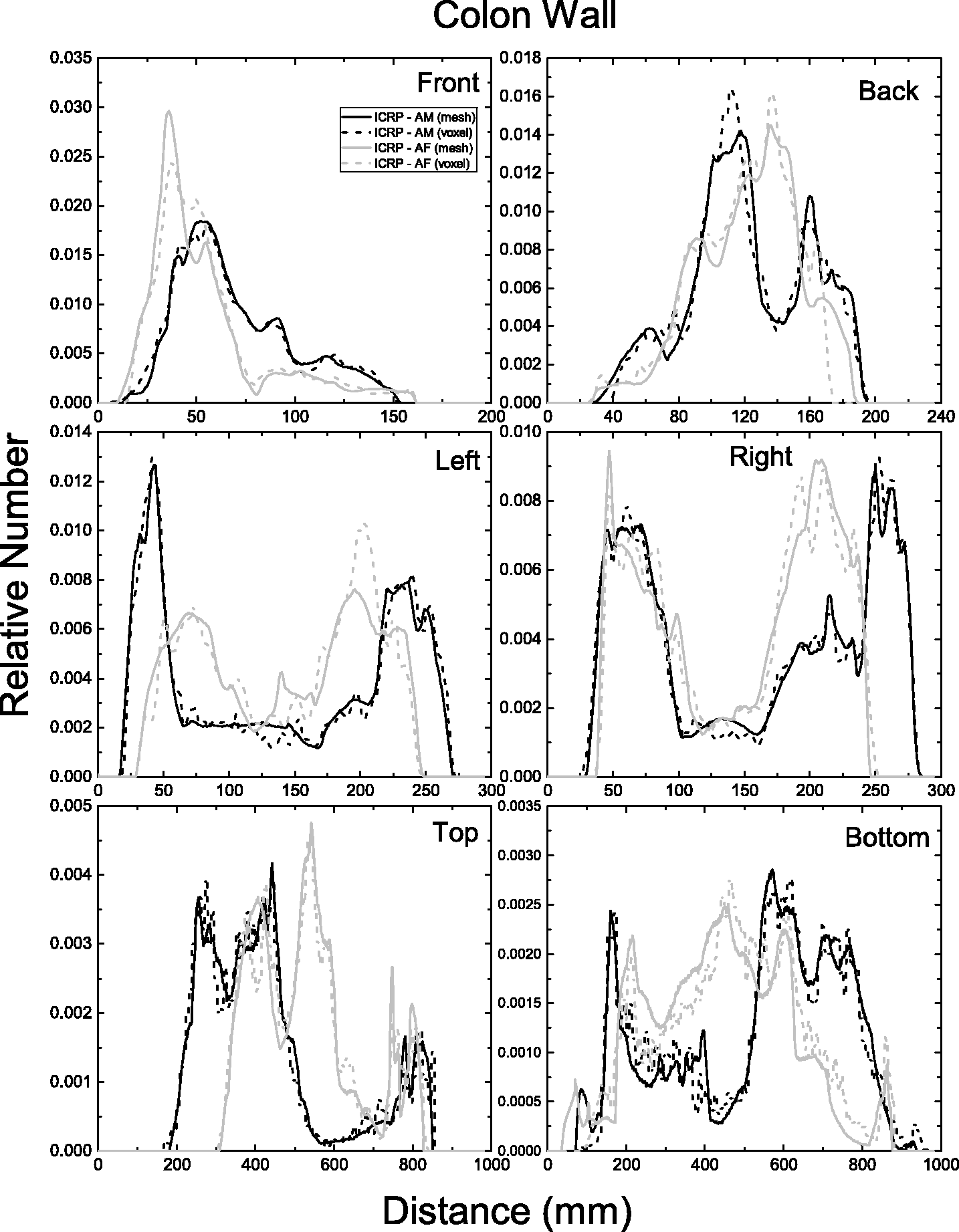
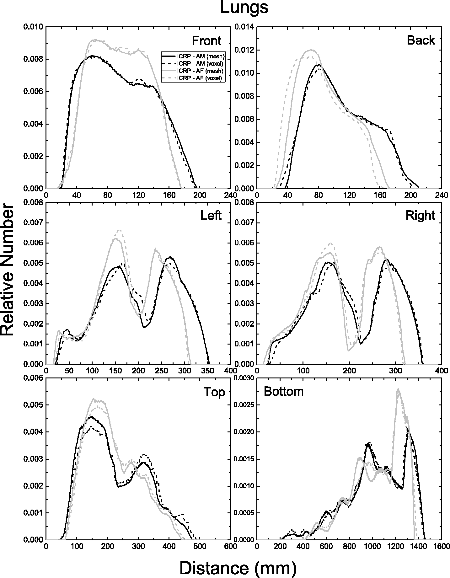
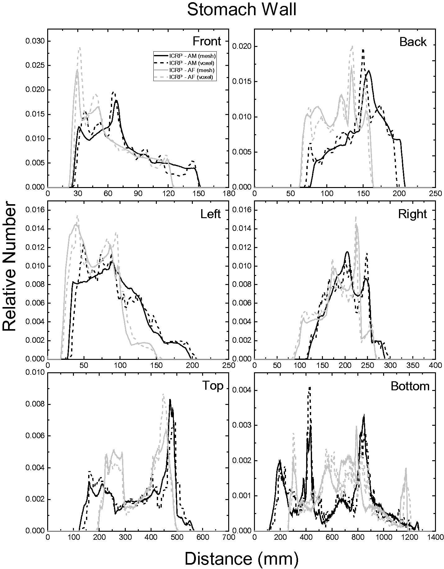
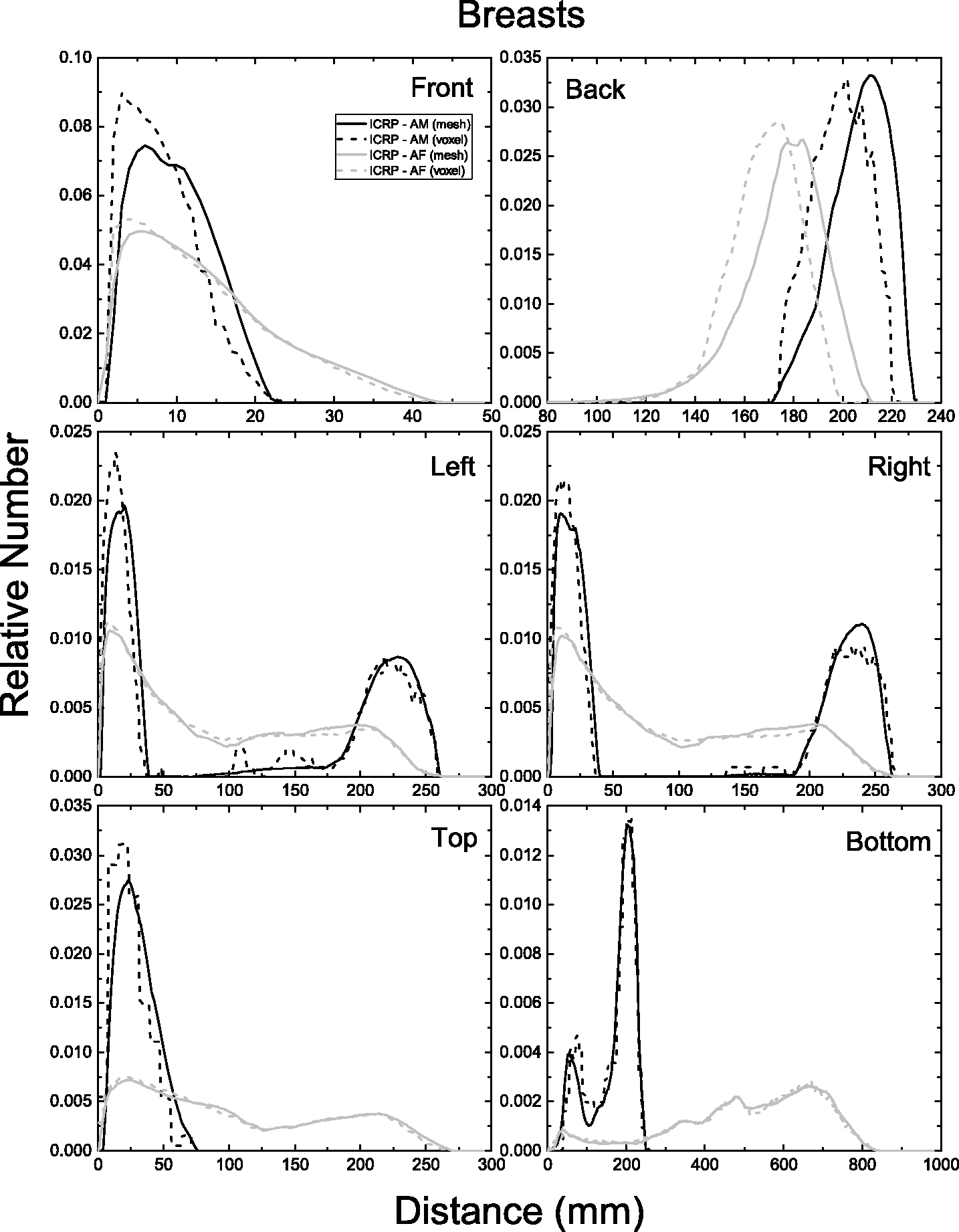
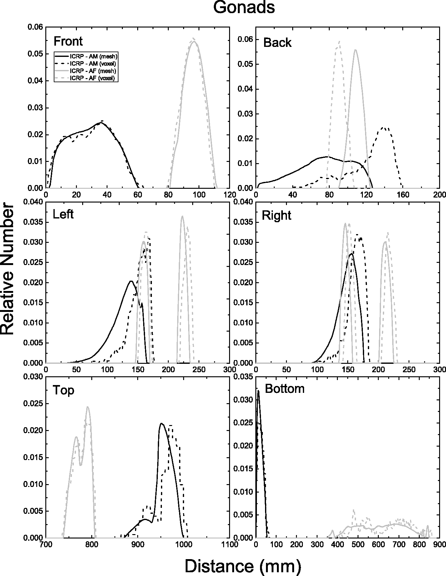
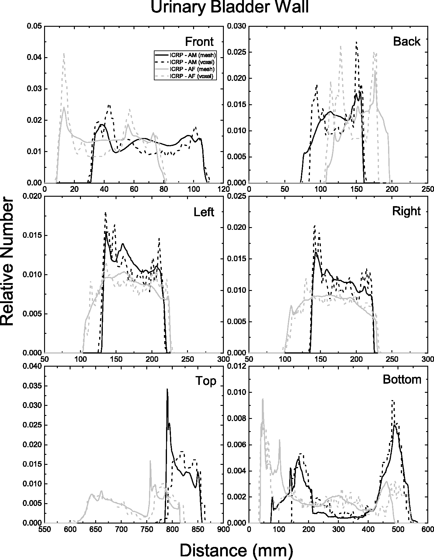
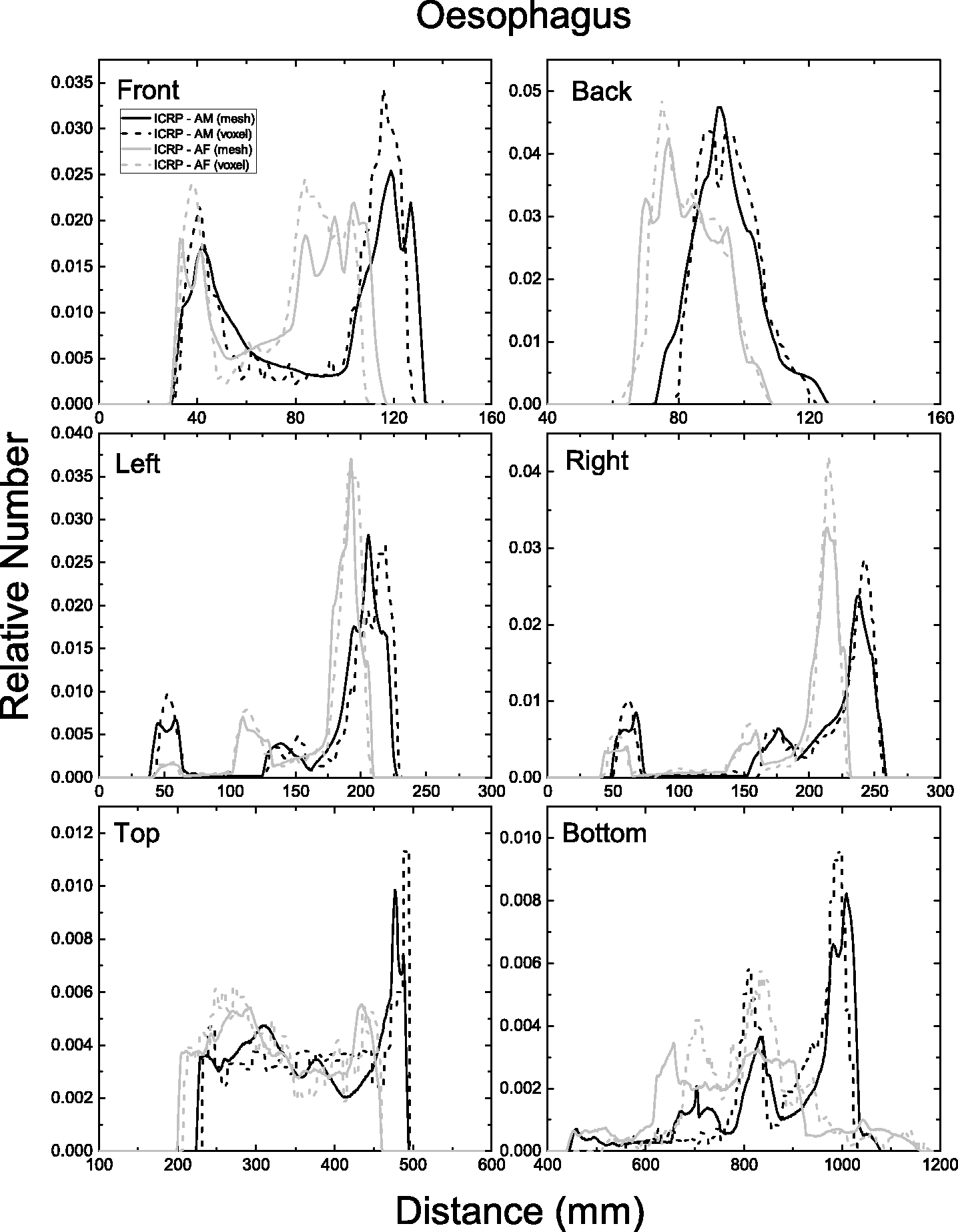
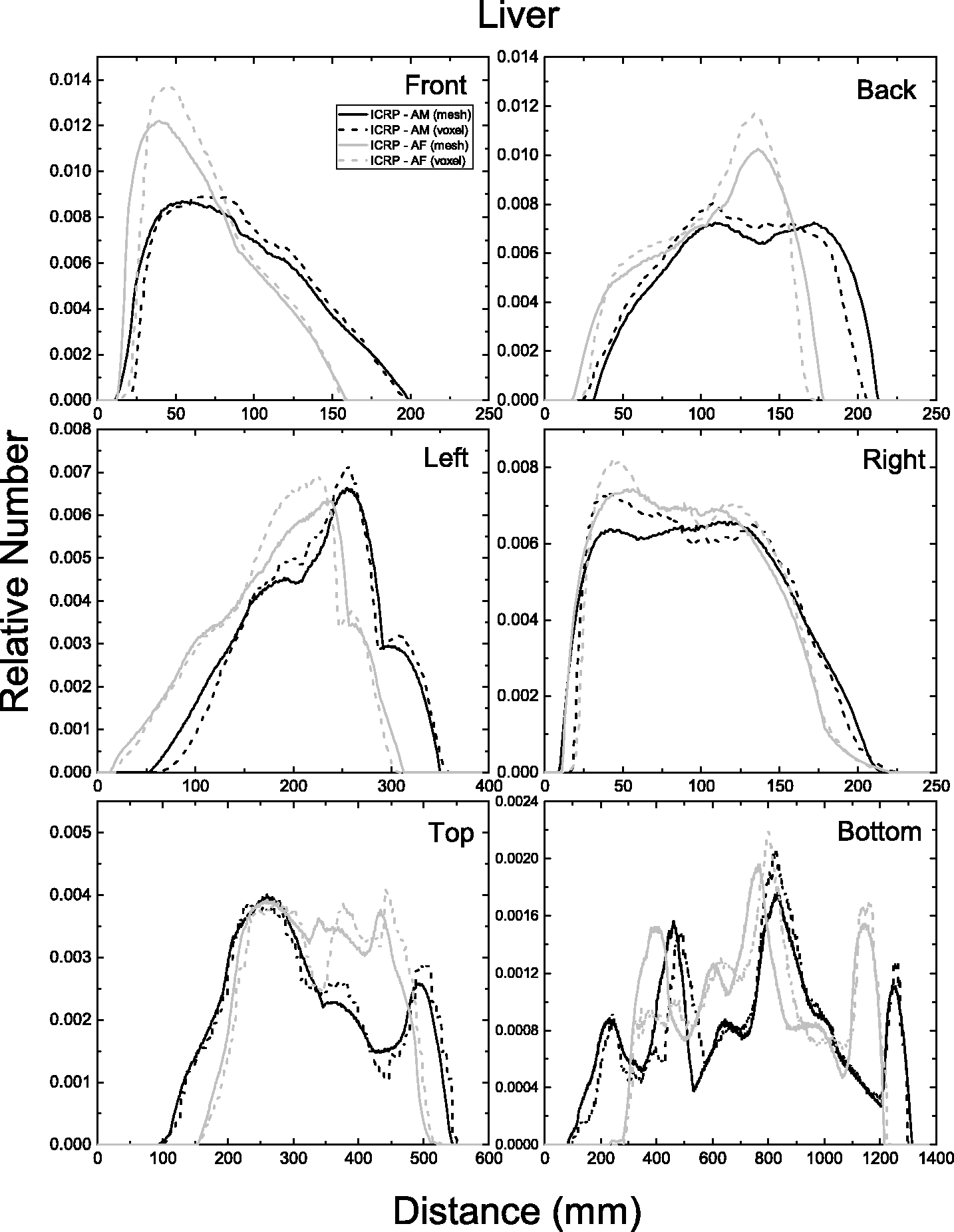
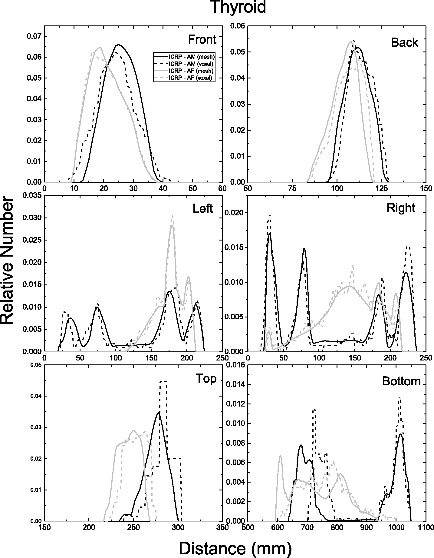
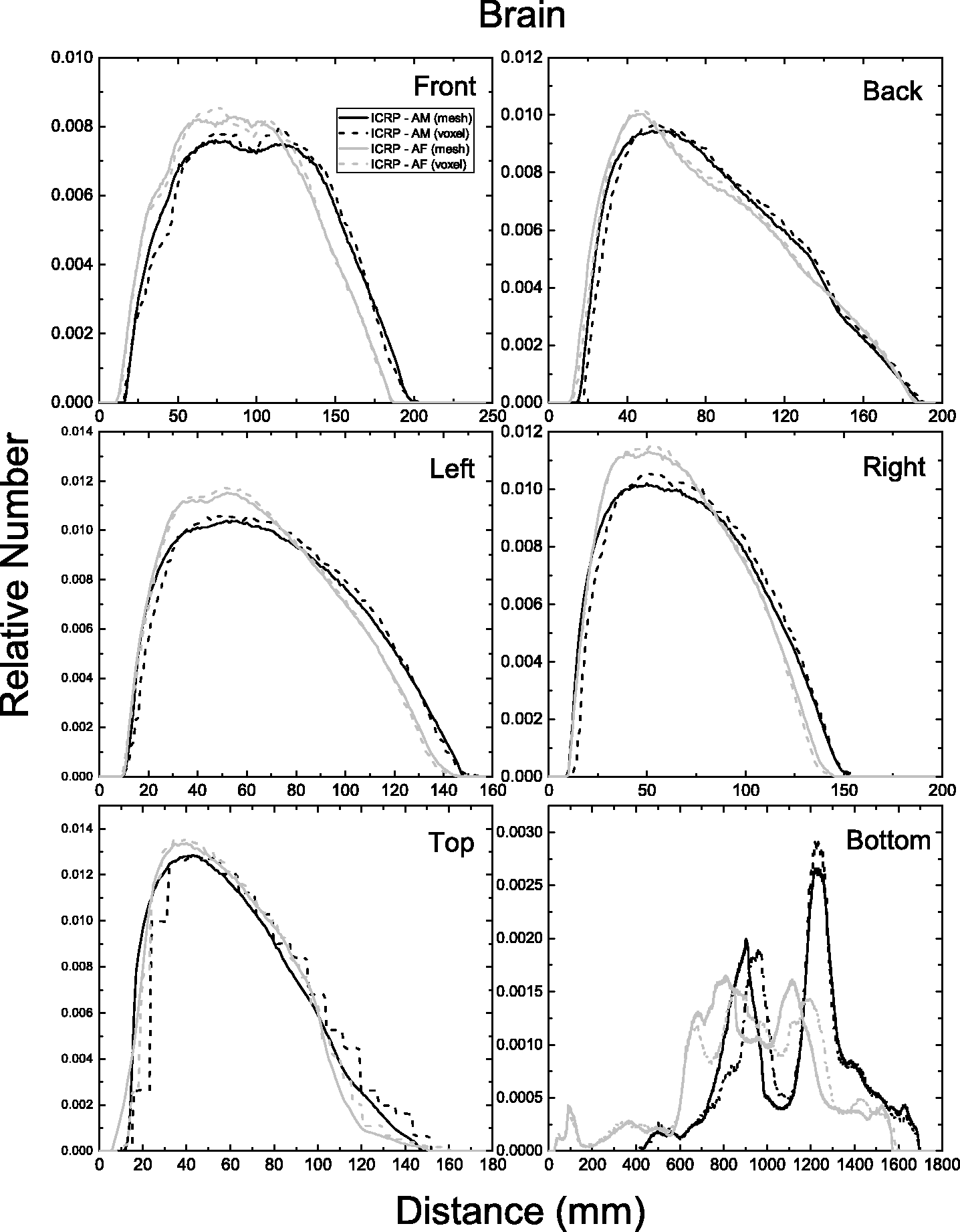
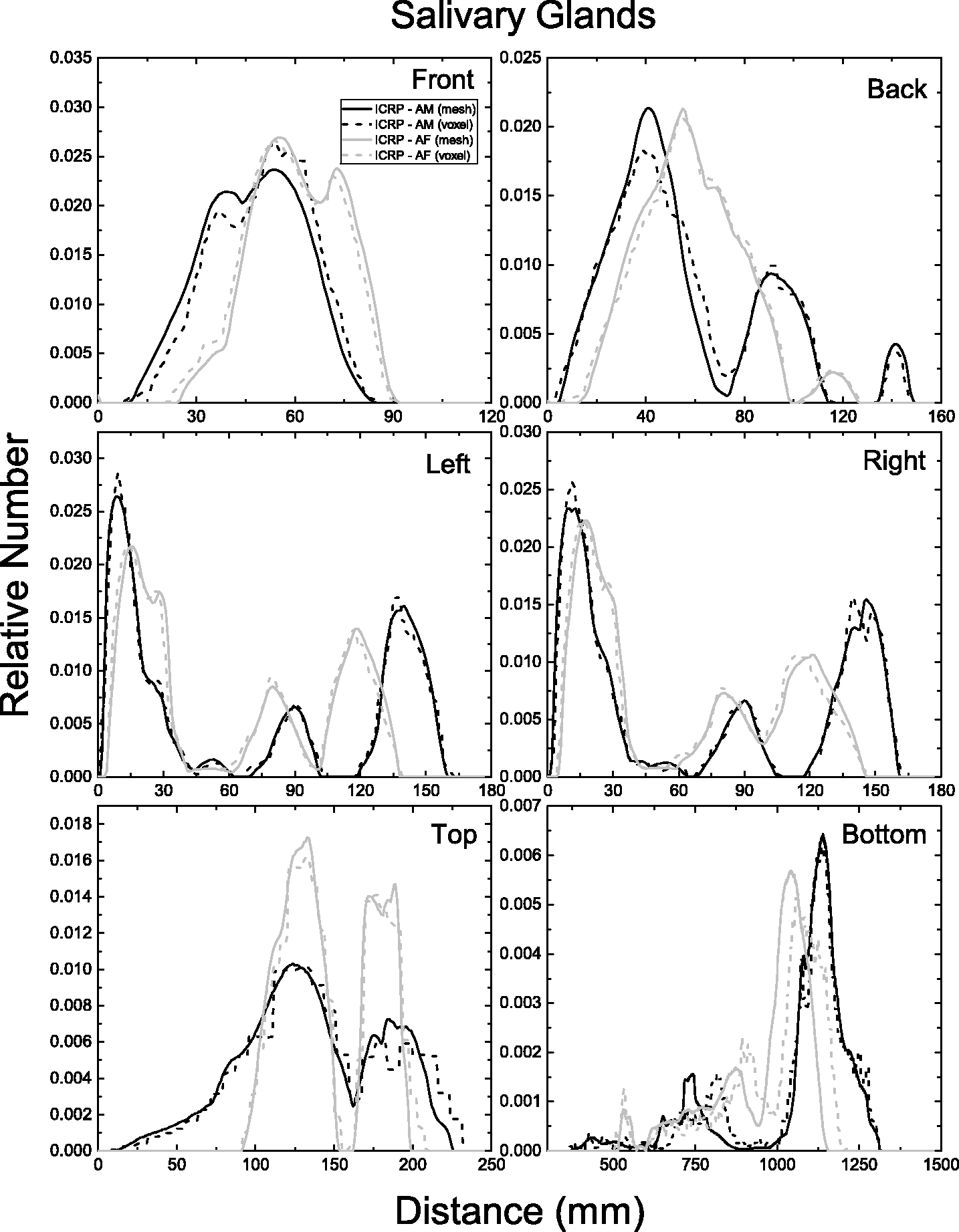
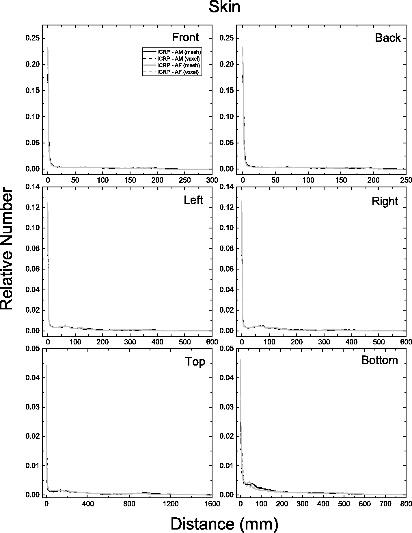
ANNEX F. CHORD LENGTH DISTRIBUTIONS BETWEEN SELECTED ORGAN PAIRS (SOURCE/TARGET TISSUES)
(F1) In Figs F.1–F.5, CLDs of the adult MRCPs and the Publication 110 (ICRP, 2009) phantoms are shown for selected organ/tissue pairs (i.e. source/target regions): source regions (cortical bone, liver, lungs, thyroid, and urinary bladder contents); target regions (RBM, colon wall, lungs, stomach wall, breasts, gonads, urinary bladder wall, oesophagus, liver, thyroid, brain, and salivary glands). For the CLD calculation, 10 million point pairs were sampled at random in the target and source regions considered, and distances of the point pairs were calculated. The CLDs represent a distance between the target and source regions, significantly influencing dose calculation for internal exposure. Distribution of distances between 10 million randomly sampled point pairs in the cortical bone (source region) and the red bone marrow (RBM), colon wall, lungs, stomach wall, breasts, gonads, urinary bladder wall, oesophagus, liver, thyroid, brain, and salivary glands (target regions). Distribution of distances between 10 million randomly sampled point pairs in the liver (source region) and the red bone marrow (RBM), colon wall, lungs, stomach wall, breasts, gonads, urinary bladder wall, oesophagus, liver, thyroid, brain, and salivary glands (target regions). Distribution of distances between 10 million randomly sampled point pairs in the lungs (source region) and the red bone marrow (RBM), colon wall, lungs, stomach wall, breasts, gonads, urinary bladder wall, oesophagus, liver, thyroid, brain, and salivary glands (target regions). Distribution of distances between 10 million randomly sampled point pairs in the thyroid (source region) and the red bone marrow (RBM), colon wall, lungs, stomach wall, breasts, gonads, urinary bladder wall, oesophagus, liver, thyroid, brain, and salivary glands (target regions). Distribution of distances between 10 million randomly sampled point pairs in the urinary bladder contents (source region) and the red bone marrow (RBM), colon wall, lungs, stomach wall, breasts, gonads, urinary bladder wall, oesophagus, liver, thyroid, brain, and salivary glands (target regions).
ANNEX G. CROSS-SECTIONAL IMAGES
ANNEX H. COMPARISON OF DOSE COEFFICIENTS FOR EXTERNAL EXPOSURE
(H1) In order to investigate the impact of the improved morphology of the adult MRCPs on the calculation of DCs for external exposures, the DCs for effective dose in terms of effective dose per fluence (pSv cm2) were calculated using the MRCPs and subsequently compared with the reference values given in Publication 116 (ICRP, 2010) that were produced with the Publication 110 (ICRP, 2009) phantoms. For these calculations, a broad parallel beam of photons, neutrons, electrons, and helium ions was assumed to be incident to the phantoms in the same irradiation geometries as considered in Publication 116. Three Monte Carlo simulation codes – Geant4 (Version 10.02), PHITS (Version 2.92), and MCNP6 (Version 2.0) – were used in the calculations. The Geant4 code was used for all of the energy points considered for the comparison, while the PHITS and MCNP6 codes were only used for some energy points for spot-check purposes. In order to facilitate the analysis, the effective dose DCs were also calculated using the Publication 110 phantoms and the Geant4 code. For the Geant4 code, the physics libraries of G4EmLivermorePhysics and FTFP_BERT_HP were used to transport all particles (Geant4 Physics Reference Manual). In addition, the thermal neutron scattering treatment S(α, β) for hydrogen (H) in light water at 300 K was applied for accurate transport of thermal neutrons. A range of 1 µm for the secondary production cut was applied to all particles. For both the PHITS and MCNP6 codes, the default physics models and cross-section data were used to transport all particles, and the thermal neutron scattering treatment was also applied. For the MCNP6 code, the default cut energies were used, which were also applied to set cut energies for the PHITS code. Note that absorbed doses to the skeletal target tissues (RBM and endosteum) were taken as the mass-weighted average of the regional spongiosa and medullary cavity doses following the same approach used in Publication 116.
ANNEX I. COMPARISON OF SPECIFIC ABSORBED FRACTIONS
(I1) In order to investigate the impact of the improved internal morphology of the adult MRCPs on the calculation of DCs for internal exposures, the SAFs for photons and electrons were calculated using the MRCPs for comparison with the values in Publication 133 (ICRP, 2016). For the calculations, the cortical bone, liver, lungs, and thyroid were selected as source organs/tissues. The Geant4 code (Version 10.02) was used for all the energy points considered for the comparison, while the PHITS (Version 2.92) and MCNP6 (Version 2.0) codes were only used for some energies for spot-check purposes. The SAFs were also calculated using the Publication 110 (ICRP, 2009) phantoms and the Geant4 code to facilitate the analysis. For the Geant4 code, the physics library of the G4EmLivermorePhysics was used to transport photons and electrons with a range of 1 µm for the secondary production cut (Geant4 Physics Reference Manual). For both the PHITS and MCNP6 codes, the default physics models and cross-section data were used to transport photons and electrons. For the MCNP6 code, the default cut energies were used, which were also applied to set cut energies for the PHITS code. Note that for photons, absorbed doses to the RBM and endosteum were calculated based on the fluence-to-absorbed-dose–response functions reported in Annex D of Publication 116 (ICRP, 2010) as recommended in Section 4.4 of Publication 133. (I2) The SAFs of the MRCPs were compared with the Publication 133 (2016) values for six target organs/tissues which were selected considering the contribution to effective dose. Figs I.1–I.8 present the SAFs of the MRCPs for the selected source and target organs/tissues for photons and electrons, along with the Publication 133 values and the values calculated with the Publication 110 (ICRP, 2009) phantoms and the Geant4 code. The statistical errors of the calculated values presented in the figures are <5%. (I3) For photons, it can be seen that the SAFs of the MRCPs are generally not much different from the Publication 133 (ICRP, 2016) values. Large differences, however, can be seen when the RBM is a target, where the SAFs of the MRCPs are much smaller than the Publication 133 values at low energies. These differences are mainly due to the fact that in the MRCPs, the spongiosa is fully enclosed by cortical bone, whereas this is not the case in the voxel-type Publication 110 (ICRP, 2009) reference phantoms (see Fig. 6.5). Even for the cortical bone as a source and the colon as a target, the SAFs show large differences, for which the values of the MRCPs are greater by a factor of ∼5 at 0.01 MeV for the male phantom, which is again due to the difference in the distribution of cortical bone; that is, in the Publication 110 phantoms, the cortical bone does not fully enclose the spongiosa and is not distributed uniformly, especially in the ribs where the cortical bone is rarely distributed in the regions that are very close to the colon. (I4) For electrons, it can be seen that the SAFs of the MRCPs are close to the Publication 133 (ICRP, 2016) values for self-irradiation cases (e.g. liver ← liver), whereas for cross-fire-irradiation cases (e.g. RBM ← liver), the SAFs show significant differences. For most of the cross-fire-irradiation cases, the SAFs of the MRCPs are generally smaller than the Publication 133 values, mainly due to the fact that the contact area between the adjacent source and target organs/tissues of the MRCPs (smooth surfaces) is smaller than that of the Publication 110 (ICRP, 2009) phantoms (stair-stepped surfaces, see Fig. 6.3). The differences were even larger when the thyroid is a source and the oesophagus and the thymus are a target, mainly due to the fact that the MRCPs overcome an anatomical limitation of the Publication 110 phantoms wherein the thyroid slightly contacts the oesophagus for both the male and the female, and the thymus for the male (see Section 3.1). Larger differences can also be seen for the RBM as a target, which is due to the fact that in the MRCPs, the cortical bone fully encloses the spongiosa, whereas this is not the case in the Publication 110 phantoms. Exceptionally, the SAFs of the MRCPs are generally greater than the Publication 133 values for the colon ← cortical bone case, which is again due to the fact that in the Publication 110 phantoms, the cortical bone is not distributed uniformly, especially in the ribs where the cortical bone is rarely distributed in the regions that are very close to the colon. Specific absorbed fractions for cortical bone as a source and red bone marrow (RBM), colon, alveolar-interstitium (AI), endosteum, brain, and muscle as a target for photon exposures calculated with the adult mesh-type reference computational phantoms MRCPs, along with the Publication 133 (ICRP, 2016) values and the values calculated with the Publication 110 (ICRP, 2009) phantoms and the Geant4 code: adult male, AM (upper) and adult female, AF (lower). Specific absorbed fractions for liver as a source and liver, colon, alveolar-interstitium (AI), stomach, gallbladder, and red bone marrow (RBM) as a target for photon exposures calculated with the adult mesh-type reference computational phantoms (MRCPs), along with the Publication 133 (ICRP, 2016) values and the values calculated with the Publication 110 (ICRP, 2009) phantoms and the Geant4 code: adult male, AM (upper) and adult female, AF (lower). Specific absorbed fractions for lungs as a source and alveolar-interstitium (AI), red bone marrow (RBM), stomach, heart, liver, and spleen as a target for photon exposures calculated with the adult mesh-type reference computational phantoms (MRCPs), along with the Publication 133 (ICRP, 2016) values and the values calculated with the Publication 110 (ICRP, 2001) phantoms and the Geant4 code: adult male (AM) (upper) and adult female (AF) (lower). Specific absorbed fractions for thyroid as a source and thyroid, red bone marrow (RBM), oesophagus, thymus, extrathoracic (ET) region, and alveolar-interstitium (AI) as a target for photon exposures calculated with the adult mesh-type reference computational phantoms (MRCPs), along with the Publication 133 (ICRP, 2016) values and the values calculated with the Publication 110 (ICRP, 2009) phantoms and the Geant4 code: adult male (AM) (upper) and adult female (AF) (lower). Specific absorbed fractions (SAFs) for cortical bone as a source and colon, alveolar-interstitium (AI), brain, and muscle as a target for electron exposures calculated with the adult mesh-type reference computational phantoms (MRCPs), along with the Publication 133 (ICRP, 2016) values and the values calculated with the Publication 110 (ICRP, 2009) phantoms and the Geant4 code: adult male (AM) (upper) and adult female (AF) (lower). Note that SAFs for the red bone marrow and endosteum as a target are not given here because these values of Publication 133 were not calculated using the Publication 110 phantoms but using the absorbed fractions calculated using the micro-computed-tomography imaging data for 38 cored samples of spongiosa provided by Hough et al. (2011). Specific absorbed fractions for liver as a source and liver, colon, alveolar-interstitium (AI), stomach, gallbladder, and red bone marrow (RBM) as a target for electron exposures calculated with the adult mesh-type reference computational phantoms (MRCPs), along with the Publication 133 (ICRP, 2016) values and the values calculated with the Publication 110 (ICRP, 2009) phantoms and the Geant4 code: adult male (AM) (upper) and adult female (AF) (lower). Specific absorbed fractions for lungs as a source and alveolar-interstitium (AI), red bone marrow (RBM), stomach, heart, liver, and spleen as a target for electron exposures calculated with the adult mesh-type reference computational phantoms (MRCPs), along with the Publication 133 (ICRP, 2016) values and the values calculated with the Publication 110 (ICRP, 2009) phantoms and the Geant4 code: adult male (AM) (upper) and adult female (AF) (lower). Specific absorbed fractions for thyroid as a source and thyroid, red bone marrow (RBM), oesophagus, thymus, extrathoracic (ET) region, and alveolar-interstitium (AI) as a target for electron exposures calculated with the adult mesh-type reference computational phantoms (MRCPs), along with the Publication 133 (ICRP, 2016) values and the values calculated with the Publication 110 (ICRP, 2009) phantoms and the Geant4 code: adult male (AM) (upper) and adult female (AF) (lower).
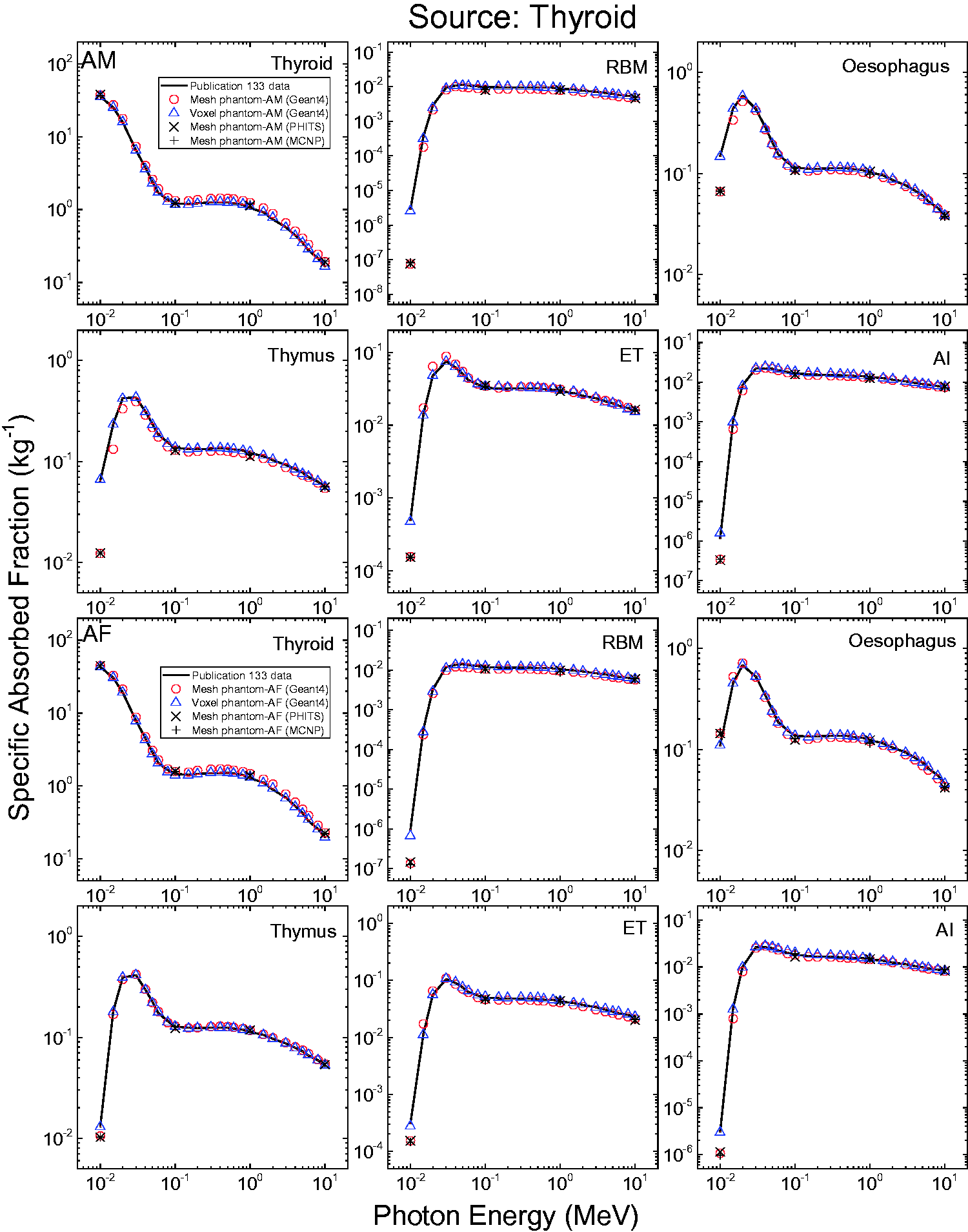
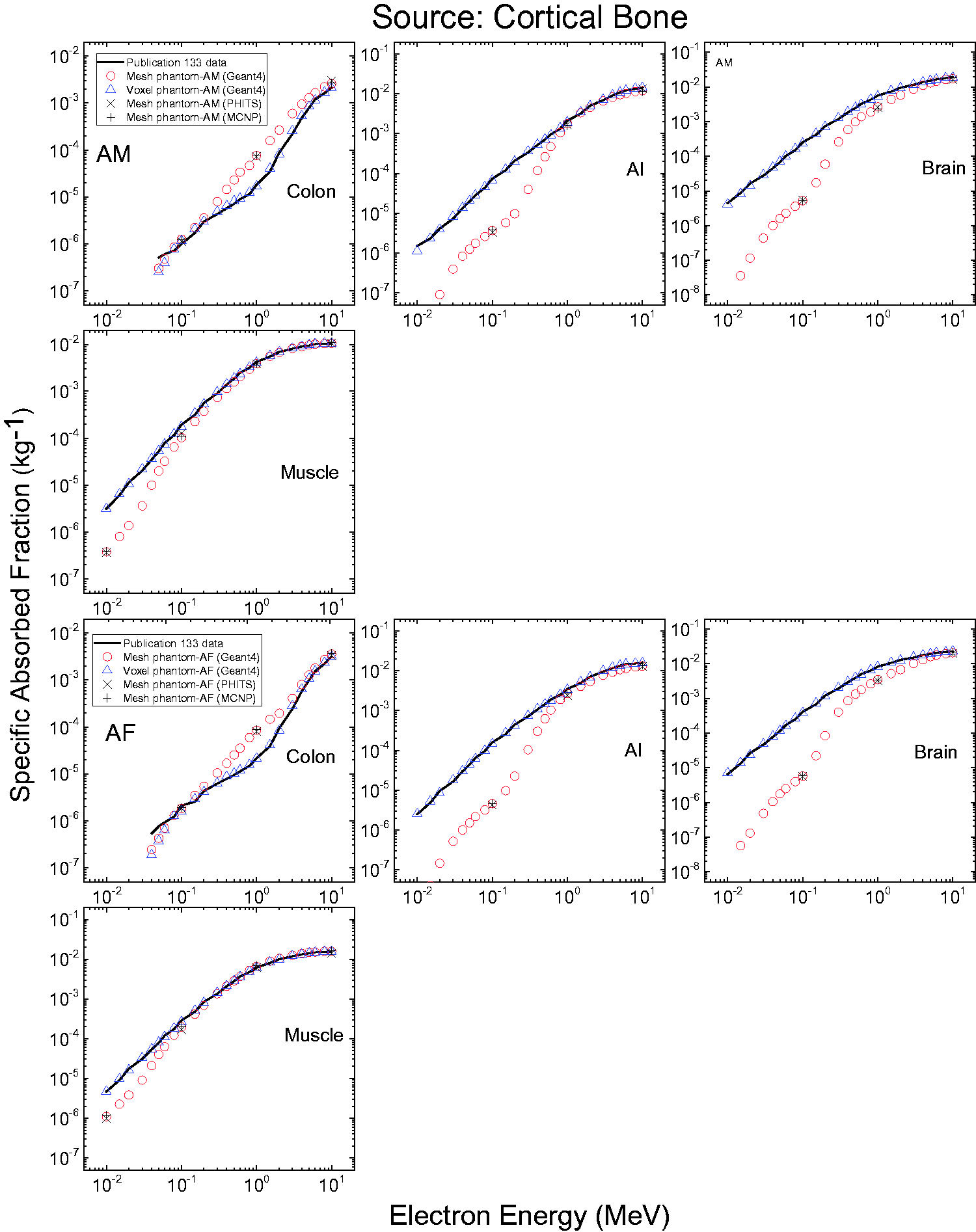
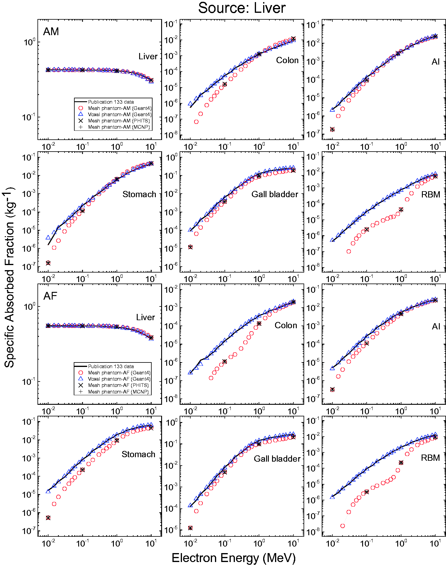
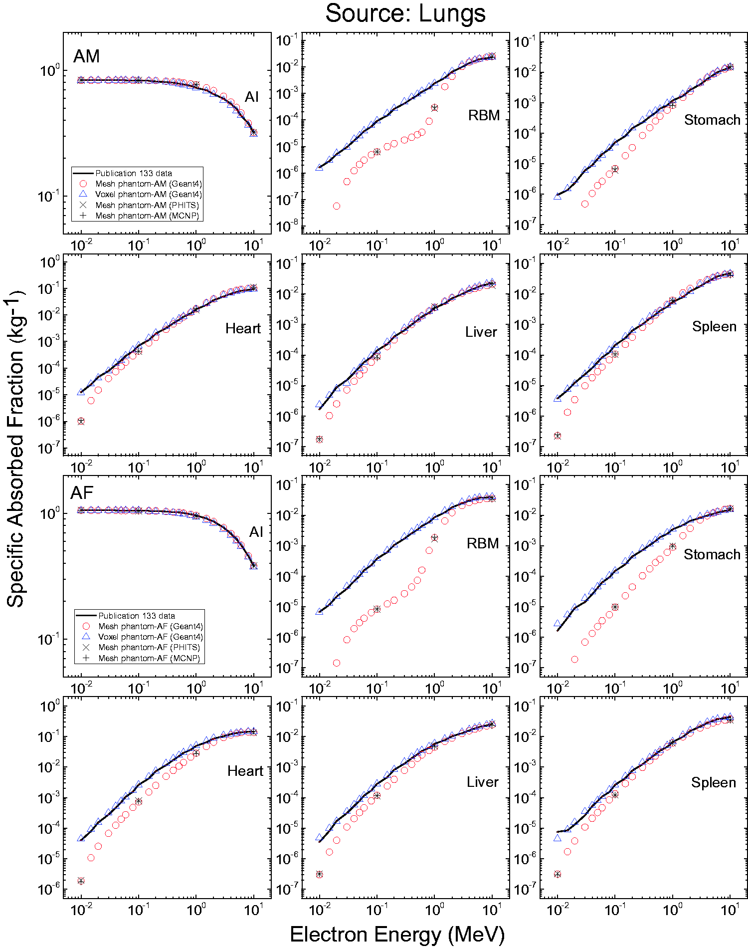
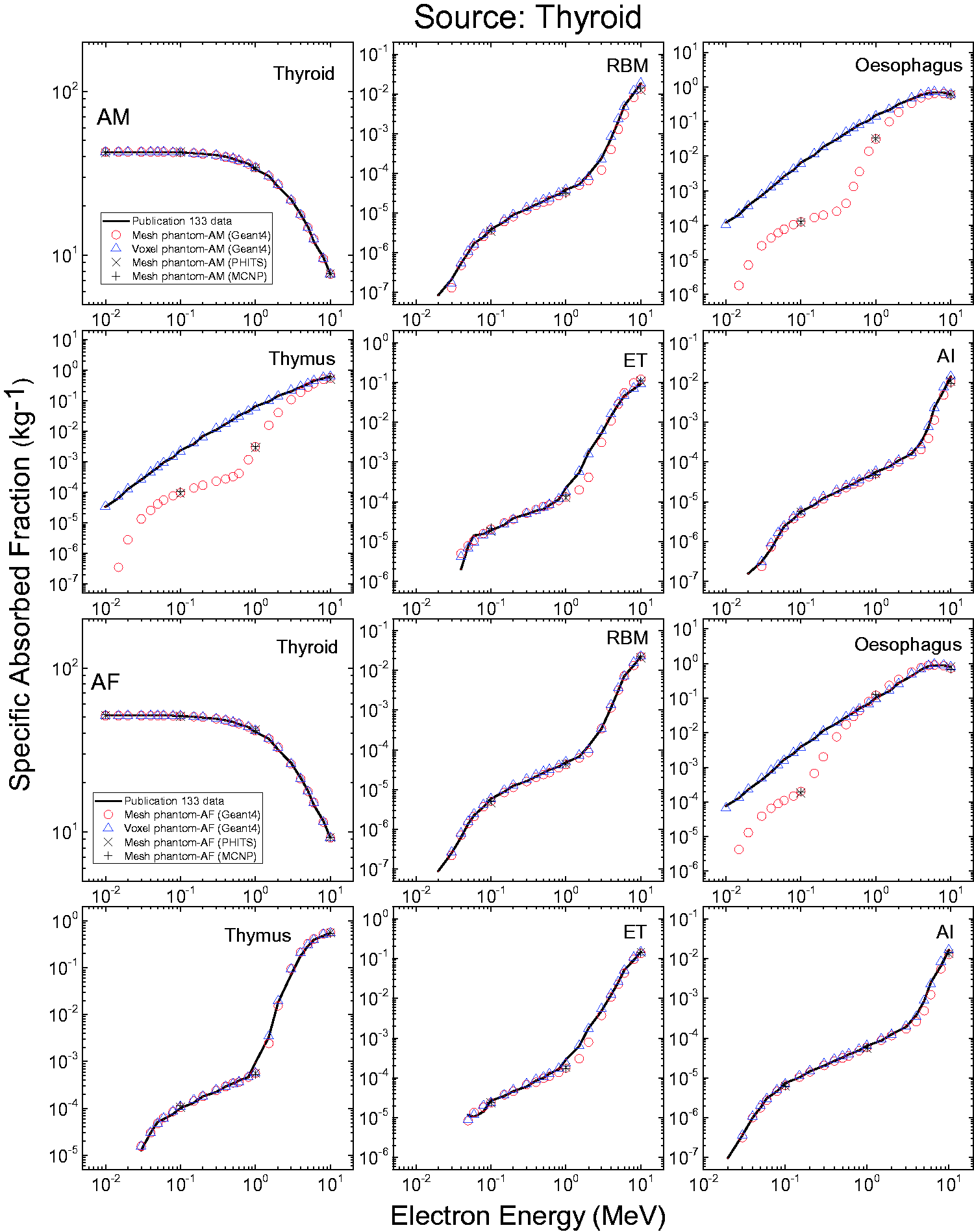
ANNEX J. DOSE COEFFICIENTS FOR INDUSTRIAL RADIOGRAPHY SOURCES
Source self-shielding factors.
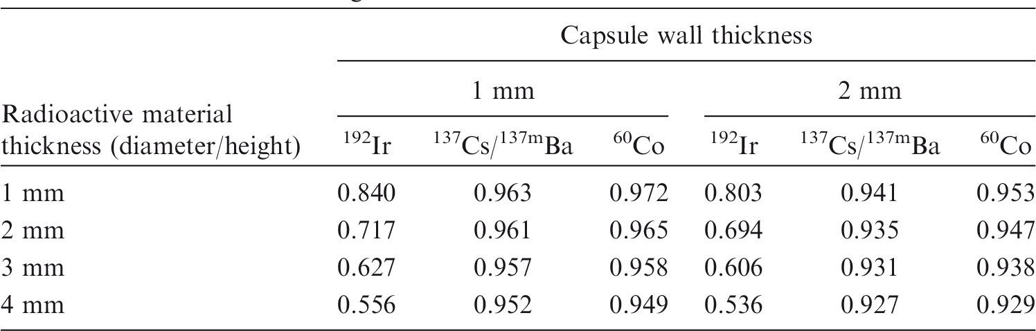
| Radioactive material thickness (diameter/height) | Capsule wall thickness |
|||||
|---|---|---|---|---|---|---|
| 1 mm |
2 mm |
|||||
| 192Ir | 137Cs/137mBa | 60Co | 192Ir | 137Cs/137mBa | 60Co | |
| 1 mm | 0.840 | 0.963 | 0.972 | 0.803 | 0.941 | 0.953 |
| 2 mm | 0.717 | 0.961 | 0.965 | 0.694 | 0.935 | 0.947 |
| 3 mm | 0.627 | 0.957 | 0.958 | 0.606 | 0.931 | 0.938 |
| 4 mm | 0.556 | 0.952 | 0.949 | 0.536 | 0.927 | 0.929 |
ANNEX K. DESCRIPTION OF ELECTRONIC FILES
(K1) The compressed package of electronic files containing the detailed data on the adult MRCPs can be found in a downloadable data file. The package is organised in two folders: Phantom_data and MC_examples.
GLOSSARY
Absorbed dose, D The absorbed dose is given by:
Absorbed fraction, AF, Fraction of energy
Active (bone) marrow Active marrow is haematopoietically active and gets its red colour from the large number of erythrocytes (red blood cells) being produced. Active bone marrow serves as a target region for radiogenic risk of leukaemia.
Activity The number of nuclear transformations of a radioactive material during an infinitesimal time interval, divided by its duration (s). The SI unit of activity is s−1 and its special name is becquerel (Bq).
Bone marrow [see also ‘Active (bone) marrow’ and ‘Inactive (bone) marrow’] Bone marrow is a soft, highly cellular tissue that occupies the cylindrical cavities of long bones and the cavities defined by the bone trabeculae of the axial and appendicular skeleton. Total bone marrow consists of a sponge-like, reticular, connective tissue framework called ‘stroma’, myeloid (blood-cell-forming) tissue, fat cells (adipocytes), small accumulations of lymphatic tissue, and numerous blood vessels and sinusoids. There are two types of bone marrow: active (red) and inactive (yellow), where these adjectives refer to the marrow’s potential for the production of blood cell elements (haematopoiesis).
Charged-particle equilibrium Charged-particle equilibrium in a volume of interest means that the energies, numbers, and directions of the charged particles are constant throughout this volume. This is equivalent to saying that the distribution of charged-particle energy radiance does not vary within the volume. In particular, it follows that the sums of the energies (excluding rest energies) of the charged particles entering and leaving the volume are equal.
Cortical (bone) marrow The marrow contained in the medullary cavities in the shafts of the long bones.
Cross-section, σ The cross-section of a target entity, for a particular interaction produced by incident charged or uncharged particles of a given type and energy, is given by:
Dose coefficient, DC A coefficient relates a dose quantity to a physical quantity, both for internal and external radiation exposure. For external exposure, the physical quantity ‘fluence’ or ‘air kerma’ is chosen. In internal dosimetry, a DC is defined as either the committed equivalent dose in tissue T per activity intake,
Dose equivalent, H The product of D and Q at a point in tissue, where D is the absorbed dose and Q is the quality factor for the specific radiation at this point, thus:
Dose–response function A particular function used in this publication to represent the absorbed dose in a target region per particle fluence in that region, derived using models of the microscopic structure of the target region geometry and the transport of the secondary ionising radiations in those regions.
Effective dose, E The tissue weighted sum of equivalent doses in all specified organs and tissues of the body, given by the expression:
Endosteum (or endosteal layer) A 50-µm-thick layer covering the surfaces of the bone trabeculae in regions of trabecular spongiosa and those of the cortical surfaces of the medullary cavities within the shafts of all long bones. It is assumed to be the target tissue for radiogenic bone cancer. This target region replaces that previously introduced in Publications 26 and 30 (ICRP, 1977, 1979) – the bone surfaces – which had been defined as a single-cell layer, 10 µm in thickness, covering the surfaces of both the bone trabeculae and the Haversian canals of cortical bone.
Equivalent dose, The equivalent dose in an organ or tissue T is given by:
Fluence, Φ The quotient of dN by da, where dN is the number of particles incident on a sphere of cross-sectional area da, thus:
Identification (ID) number Number assigned unequivocally to each individually segmented organ/tissue.
Inactive (bone) marrow In contrast to active marrow, inactive marrow is haematopoietically inactive, i.e. does not directly support haematopoiesis. It gets its yellow colour from fat cells which occupy most of the space of the yellow bone marrow framework.
Intake, I Activity that enters the body through the respiratory tract or the gastrointestinal tract or the skin. – Acute intake A single intake by inhalation or ingestion, taken to occur instantaneously. – Chronic intake Intake over a specified period of time.
LET See ‘Linear energy transfer’.
Linear energy transfer/unrestricted linear energy transfer, L or LET The quotient of dE by dl, where dE is the mean energy lost by the charged particle due to electronic interactions in traversing a distance dl, thus:
Mean absorbed dose in an organ or tissue, The mean absorbed dose in a specified organ or tissue T, is given by:
Mesh phantom Computational anthropomorphic phantom whose anatomy is represented by either the polygon mesh format or the tetrahedral mesh format.
Non-uniform rational B-spline, NURBS NURBS represents three-dimensional surface geometry by mathematical curves defined by four parameters: degree, control points, knots, and an evaluation rule. NURBS-based models are widely used in computer-aided design, manufacturing and engineering, and other three-dimensional modelling and animation applications.
Organ absorbed dose or organ dose Short phrase for ‘mean absorbed dose in an organ or tissue’.
Polygon mesh Polygon mesh represents three-dimensional surface geometry composed of polygonal facets (such as triangles), and is one of the geometry formats of a mesh phantom (see ‘Mesh phantom’).
Radiation weighting factor, A dimensionless factor by which the organ or tissue absorbed dose is multiplied to reflect the higher biological effectiveness of high-LET radiation compared with low-LET radiation. It is used to derive the equivalent dose from the absorbed dose averaged over a tissue or organ.
Red (bone) marrow See ‘Active (bone) marrow’.
Reference Male and Reference Female Reference Male and Female are defined as either adults or children of ages 0, 1, 5, 10, and 15 years.
Reference Person An idealised person for whom the equivalent doses to organs and tissues are calculated by averaging the corresponding organ doses in Reference Male and Reference Female. The equivalent doses of Reference Person are used for the calculation of effective dose.
Reference Phantom The computational phantom of the human body (male or female voxel phantom based on medical imaging data), defined in Publication 110 (ICRP, 2009), with the anatomical and physiological characteristics of Reference Male and Reference Female defined in Publication 89 (ICRP, 2002).
Reference value Value of a quantity recommended by ICRP for use in dosimetric applications or biokinetic models. Reference values are fixed and specified with no uncertainty, independent of the fact that the basis of these values includes many uncertainties.
Sievert (Sv) The special name for the SI unit of equivalent dose, effective dose, and operational dose quantities. The unit is J kg−1.
Source An entity for which radiological protection can be optimised as an integral whole, such as the x-ray equipment in a hospital, or the release of radioactive material from an installation. Sources of radiation, such as radiation generators and sealed radioactive materials, and, more generally, the cause of exposure to radiation or to radionuclides.
Source region, An anatomical region within the reference phantom body which contains the radionuclide following its intake. The region may be an organ, a tissue, the contents of the gastrointestinal tract or urinary bladder, or the surfaces of tissues as in the skeleton, the alimentary tract, and the respiratory tract.
Specific absorbed fraction, SAF The fraction of energy of that emitted as a specified radiation type in a source region, S, that is absorbed per mass of target tissue, T (kg−1).
Spongiosa Term referring to the combined tissues of the bone trabeculae and marrow tissues (both active and inactive) located within cortical bone cortices across regions of the axial and appendicular skeleton. Spongiosa is one of three bone regions defined in the Publication 110 reference phantoms (ICRP, 2009), the other two being cortical bone and medullary marrow of the long bone shafts. As the relative proportions of trabecular bone, active marrow, and inactive marrow vary with skeletal site, the homogeneous elemental composition and mass density of spongiosa are not constant but vary with skeletal site [see Annex B of Publication 110 (ICRP, 2009)].
Stem cell Non-differentiated, pluripotent cell, capable of unlimited cell division.
Stochastic effects of radiation Malignant disease and heritable effects for which the probability of an effect occurring, but not its severity, is regarded as a function of dose without threshold.
Target region, A tissue region of the body in which a radiation absorbed dose or equivalent dose is received.
Target tissue, T Organ or tissue in the body for which tissue weighting factors are assigned in the effective dose (ICRP, 1991, 2007). In many cases, each target tissue T corresponds to a single target region
Tetrahedral mesh Tetrahedral mesh represents three-dimensional geometry composed of tetrahedrons, which is one of the geometry formats of a mesh phantom (see ‘Mesh phantom’). Tetrahedral mesh can be generated by subdividing polygon mesh (see ‘Polygon mesh’) with tetrahedrons.
Tissue reaction Injury in populations of cells, characterised by a threshold dose and an increase in the severity of the reaction as the dose is increased further. Also termed ‘deterministic effect’. In some cases, these effects are modifiable by postirradiation procedures including biological response modifiers.
Tissue weighting factor, The factor by which the equivalent dose in an organ or tissue T is weighted to represent the relative contribution of that organ or tissue to overall radiation detriment from stochastic effects (ICRP, 1991, 2007). It is defined such that:
Trabecular (bone) marrow The marrow contained in the spongiosa regions of all bones.
Voxel phantom Computational anthropomorphic phantom based on medical tomographic images or photographic images of a cadaver in which the anatomy is described by small three-dimensional volume elements (voxels) specifying the organ or tissue to which they belong.
Yellow (bone) marrow See ‘Inactive (bone) marrow’.
References
ICRP, 1977. Recommendations of the International Commission on Radiological Protection. ICRP Publication 26. Ann. ICRP 1(3).
ICRP, 1979. Limits for Intakes of Radionuclides by Workers. Part 1. ICRP Publication 30. Ann. ICRP 2 (3/4).
ICRP, 1991. 1990 Recommendations of the International Commission on Radiological Protection. ICRP Publication 60. Ann. ICRP 21 (1-3).
ICRP, 2002. Basic Anatomical and Physiological Data for Use in Radiological Protection Reference Values. ICRP Publication 89. Ann. ICRP 32 (3-4).
ICRP, 2007. The 2007 Recommendations of the International Commission on Radiological Protection. ICRP Publication 103. Ann. ICRP 37 (2-4).
ICRP, 2009. Adult Reference Computational Phantoms. ICRP Publication 110. Ann. ICRP 39 (2).
ACKNOWLEDGEMENTS
In 2013, Committee 2 initiated a project to investigate converting the current voxel phantoms of Publication 110 into high-quality mesh format including all source and target tissues in order to address limitations of the voxel phantoms. Preliminary results were presented at the ![]() Symposium held in Seoul, Korea. In the Committee 2 meeting after the symposium, it was suggested by some committee members that it would be necessary to upgrade the current ICRP paediatric phantoms to include the detailed eyes and skin, and the thin target tissues of the alimentary and respiratory tract organs. In 2016, ICRP established Task Group 103 on Mesh-type Reference Computational Phantoms (MRCPs) to complete this work. The present report is the first publication of Task Group 103, presenting adult MRCPs. A second report will present the paediatric MRCPs.
Symposium held in Seoul, Korea. In the Committee 2 meeting after the symposium, it was suggested by some committee members that it would be necessary to upgrade the current ICRP paediatric phantoms to include the detailed eyes and skin, and the thin target tissues of the alimentary and respiratory tract organs. In 2016, ICRP established Task Group 103 on Mesh-type Reference Computational Phantoms (MRCPs) to complete this work. The present report is the first publication of Task Group 103, presenting adult MRCPs. A second report will present the paediatric MRCPs.
ICRP thanks all those involved in the development of this publication for their hard work and dedication over many years.

| C.H. Kim (Chair) | H.S. Kim | M. Zankl |
| W.E. Bolch | C. Lee | |
| C. Choi | T.T. Nguyen | |
| B.S. Chung | N. Petoussi-Henss | |
| K. Eckerman | R. Qiu | |
| M.C. Han | Y.S. Yeom |

| H. Han | B. Shin |

| D. Nosske | L. Bertelli |

| K. Cho | S. Liu |
C.H. Clement (Scientific Secretary and Annals of the ICRP Editor-in-Chief)
H. Fujita (Assistant Scientific Secretary and Annals of the ICRP Associate Editor)

| J.D. Harrison (Chair) | D. Chambers | J. Ma |
| F. Paquet (Vice-Chair) | M. Degteva | D. Nosske |
| W.E. Bolch (Secretary) | A. Endo | N. Petoussi-Henss |
| M.R. Bailey | J.G.S. Hunt | F. Wissmann |
| V. Berkovski | C.H. Kim | |
| L. Bertelli | R. Leggett |

| J.D. Harrison (Chair) | D. Jokisch | T. Sato |
| F. Paquet (Vice-Chair) | C.H. Kim | T. Smith |
| W.E. Bolch (Secretary) | R. Leggett | A. Ulanowski |
| V. Berkovski | J. Li | F. Wissmann |
| E. Blanchardon | M.A. Lopez | |
| A. Giussani | N. Petoussi-Henss |
K. Eckerman
Chair: C. Cousins, UK
Vice-Chair: J. Lochard, France
| K.E. Applegate, USA | S. Liu, China |
|
| S. Bouffler, UK | S. Romanov, Russia | R.H. Clarke, UK |
| K.W. Cho, Korea | W. Rühm, Germany | F.A. Mettler Jr, USA |
| D.A. Cool, USA | R.J. Pentreath, UK | |
| J.D. Harrison, UK | R.J. Preston, USA | |
| M. Kai, Japan | C. Streffer, Germany | |
| C-M. Larsson, Australia | E. Vañó, Spain | |
| D. Laurier, France |
†Although formally not a member since 1988, the Scientific Secretary is an integral part of the Main Commission.
Finally, thank you very much to all organisations and individuals who took the time to provide comments on the draft of this publication during the consultation process.
References
Supplementary Material
Please find the following supplemental material available below.
For Open Access articles published under a Creative Commons License, all supplemental material carries the same license as the article it is associated with.
For non-Open Access articles published, all supplemental material carries a non-exclusive license, and permission requests for re-use of supplemental material or any part of supplemental material shall be sent directly to the copyright owner as specified in the copyright notice associated with the article.