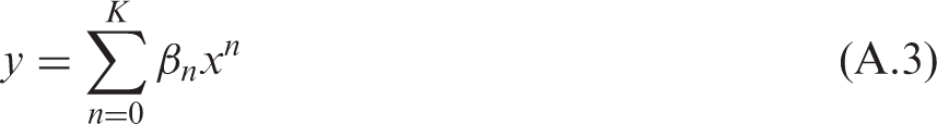
Abstract
Guest Editorial
Extending the Breadth and Depth of Dosimetry for Biota in an Environmental Context
When the International Commission on Radiological Protection (ICRP) first embarked on the task of providing advice on protection of the environment under different exposure situations, it did so by drawing on the best of the rather limited information available at that time. However, in doing so, it also considered that if a framework could be set out that had, admittedly, significant gaps and deficiencies within it, others might recognise the merit of such an approach and thus contribute to making it more complete. The present publication is another welcome step in that direction.
The basis of ICRP’s framework is to draw together a few internally consistent data sets on the relationships between exposure and dose, and dose and effect, for a few types of plants and animals typical of different environments – the Reference Animals and Plants (RAPs). Such data sets can then be used, quite literally, as points of reference for other evaluations, or simply as default values, as required. However, in real-world situations, the actual plants and animals exposed, the Representative Organisms (ROs), are the objects of interest; these organisms could be almost anything, and it is therefore necessary to estimate the doses received by them, and then to compare such data with the nearest relevant RAP data in order to evaluate the likely radiation effects for such organisms in an environmental context.
In Publication 108 (ICRP, 2008a), on the concept and use of RAPs, a set of dose conversion factors for the RAPs was provided in Annex C. The terminology used was quite deliberate, in order not to confuse such tabulated values with those that were used for human radiological protection. The data sets were rather limited, and pragmatic decisions had to be made to constrain the range of parameters included. However, now that the concept of extending the remit of radiological protection beyond that of the human being has become more generally accepted, it seems sensible to use the same terminology, and the values in this publication are therefore given as dose coefficients (DCs). These DCs for animals and plants have also been brought up to date by being based on the nuclear decay data of Publication 107 (ICRP, 2008b). They have also been set out in a way that many will find more useful, on a nuclide-by-nuclide basis, and they are again broken down into fractions to represent the contributions of fission fragments and alpha-recoil nuclei, alpha particles, and low-energy (<10 keV) and high-energy (>10 keV) beta and gamma radiation.
Another factor considered in Publication 108 (ICRP, 2008a) was how best to allow for decay chains. The time frames of relevance can vary considerably from one organism to another, and the present publication provides useful guidance on how to select the most appropriate time frame for truncation.
Up until now, ICRP has not given any specific advice on how best to calculate the dose rates to the ROs; it has only provided data relevant to the RAPs. It was nevertheless assumed that use would normally be made of those databases developed through the excellent FASSET and ERICA programmes (Larsson, 2004, 2008), and these were used as the basis of the BiotaDC programme contained in this publication (Annex C).
When reading this publication, it is important to note that the tabulated information should only be applied having first taken full consideration of the various exposure situations discussed in Publication 108 (ICRP, 2008a), as well as the advice and numerical values in Publication 114 (ICRP, 2009) on transfer parameters. Thus, for example, the external DCs for aquatic organisms are given as being ‘uniform isotropic’. This condition only actually applies to truly pelagic organisms, such as the RAP trout or similar ROs. For all of the other aquatic RAPs, they do not apply. Thus, the RAP crab, seaweed, and flatfish, as well as the RAP duck, are never in a situation of uniform isotropic exposure (4π) geometry over a 24-h period. Indeed, the flatfish, virtually by definition, lives either on, or even within, the sediment, as does the crab (with many species spending some 80% of a 24-h period well beneath the surface of the sediment), and intertidal benthic algae lie on the sediment for half of their daily exposure. Indeed, even a bird like a duck, as discussed in Publication 108 (ICRP, 2008a), will be variously exposed to different sources, all in essentially 2π geometry, throughout the day. The density and chemical compositions of sediments are also very different from those of seawater, and the concentrations of some of the nuclides considered in this publication in marine sediments may be up to five or six orders of magnitude greater than those of the overlying water, thus completely dominating any estimated dose rate for such radionuclides.
The dose rates, once calculated, need to be compared with the derived consideration reference levels (DCRLs), which are given in (fractions of) Gy day−1. This time frame was chosen deliberately and carefully by ICRP as being the most relevant to environmental situations, both in terms of a dose rate and in order to estimate the total dose received by organisms over different stages of their life cycle. Hence, all of the associated biological information in Publication 108 (ICRP, 2008a) is deliberately given in ‘days’, as is the information relating to how ICRP’s system should be applied to protection of the environment under different exposure situations, as set out in Publication 124 (ICRP, 2014). In this publication, they are presented as Gy h−1 (which is the unit usually used for laboratory experiments on radiation effects and rarely of environmental relevance), and thus there is scope for error when comparing them with the DCRLs. Fig. 1.1 expresses the DCRLs using both time frames, to help both the ‘ecology’ and ‘laboratory’ communities in applying the DCs and the DCRLs judiciously.
Derived consideration reference levels (DCRLs) for environmental protection for each Reference Animal or Plant (RAP), the RAPs being grouped according to their DCRL ranges. Adapted from Fig. 3.1 of Publication 124 (ICRP, 2014a).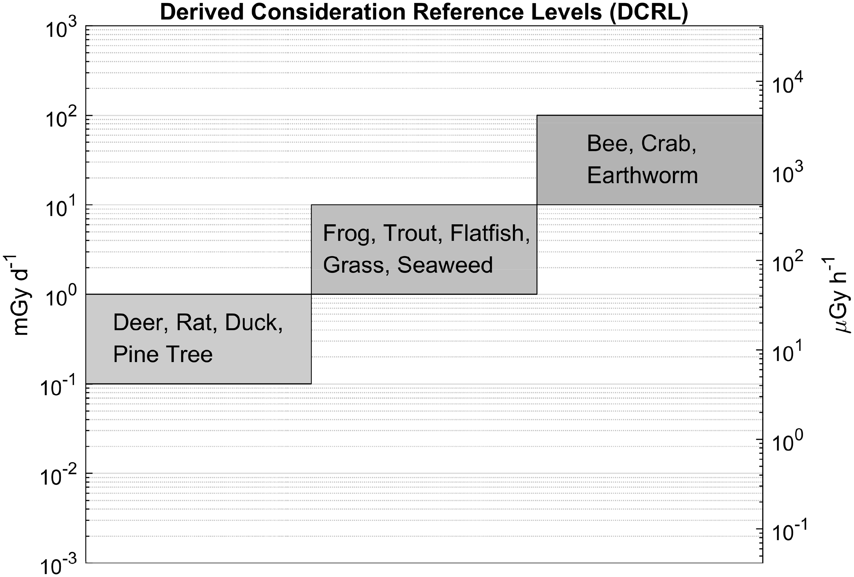
The dose models are still based on a simple geometry: spheres and ellipsoids. Such models have served well for many decades, and it is impractical to consider any other approach for the vast range of ROs that are likely to be considered in environmental evaluations. However, for the larger RAPs, the development of voxel phantoms, such as the approach being developed by Higley et al. (2015), will still be necessary in order to interpret the relationships between exposures, dose, and biological effects for different types of animals and plants. This will take some time to achieve. In the meantime, the authors of this publication are to be congratulated for taking practical dosimetry to a higher level, particularly with regard to the terrestrial environment, and for extending the DCs so that they can be applied to ROs in an internally consistent manner.
R.J. Pentreath
ICRP Main Commission Emeritus Member
References
DOSE COEFFICIENTS FOR NON-HUMAN BIOTA ENVIRONMENTALLY EXPOSED TO RADIATION
ICRP PUBLICATION 136
Approved by the Commission in May 2017
© 2017 ICRP. Published by SAGE.
Keywords: Non-human biota; Radiological protection of the environment; Dose coefficients; Reference Animals and Plants; Dosimetry
AUTHORS ON BEHALF OF ICRP
A. ULANOVSKY, D. COPPLESTONE, J. VIVES I BATLLE
PREFACE
The dosimetric approach adopted by the International Commission on Radiological Protection (ICRP) for non-human biota was summarised and presented in Publication 108 (ICRP, 2008b). Despite its extensive coverage, Publication 108 can be seen as having methodological gaps and being restricted to the family of Reference Animals and Plants. The present publication addresses such concerns and provides an extended methodology, a revised database, and a software tool for more detailed calculations.

The membership of Committee 5 during the period of preparation of this publication was:
The software tool BiotaDC (Annex C) was developed on behalf of ICRP by A. Ulanovsky and A. Ulanowski.
Helpful comments from Main Commission members J.D. Harrison and J-K. Lee, as well as efficient assistance from the former Associate Editor N. Hamada, are gratefully acknowledged.
MAIN POINTS
GLOSSARY
Absorbed dose, D (ICRU, 2011) The quotient of dɛ by dm, where dɛ is the mean energy imparted by ionising radiation to matter of mass dm. The unit of absorbed dose is J kg−1, and its special name is gray (Gy). The quotient of dEtr by dm, where dEtr is the mean sum of the initial kinetic energies of all charged particles in a mass dm of a material by the uncharged particles incident on dm. The unit of kerma is J kg−1, and its special name is gray (Gy). A band of dose rate within which there is likely to be some chance of deleterious effects of ionising radiation occurring to individuals of that type of Reference Animal or Plant (derived from a knowledge of defined expected biological effects for that type of organism) that, when considered together with other relevant information, can be used as a point of reference to optimise the level of effort expended on environmental protection, dependent upon the overall management objectives and the relevant exposure situation. A coefficient relating an absorbed dose rate in the whole body, or in a part of it, and radionuclide activity concentration in the body for internal exposure, or in the environment in the case of external exposures. In this publication, for exposure to internally distributed sources, DCs are formulated in units of dose rate (µGy h−1) per unit activity concentration in the body (Bq kg−1), while for external exposures, these dose rates are given as per unit mass (Bq kg−1), surface (Bq m−2), or volume (Bq L−1 or Bq m−3) activity concentrations. As recommended by ICRP (2007) and applied previously to dosimetric data for humans (ICRP, 2012), the term ‘dose coefficients’ replaces the previously used terms ‘dose conversion coefficients’ and ‘dose conversion factors’, thus resulting in harmonised dosimetric terminology across the ICRP publications. The product of D and Q at a point in tissue, where D is the absorbed dose and Q is the quality factor for the specific radiation at this point, thus:
The unit of dose equivalent is J kg−1, and its special name is sievert (Sv). The quotient of dN by da, where dN is the number of particles incident on a sphere of cross-sectional area da. The unit of fluence is m−2. For calculation of external doses, the occupancy factor is the fraction of time that an organism spends at a specified location in its habitat (whether underground, on the soil/sediment surface, or fully immersed in air or water). A practical method (function or numerical value) used to represent relative biological effectiveness for a specific type of radiation, based on existing scientific knowledge and adopted by consensus or via recommendations. Within the system of human radiological protection, it is used to define and derive the equivalent dose from the mean absorbed dose in an organ or tissue. A hypothetical entity, with the assumed basic biological characteristics of a particular type of animal or plant, as described to the generality of the taxonomic level of family, with defined anatomical, physiological, and life history properties, that can be used for the purposes of relating exposure to dose, and dose to effects, for that type of living organism. A theoretical concept that expresses the property of the given radiation type to affect living biological tissue. RBE is defined as the ratio of absorbed dose of a low-linear-energy-transfer reference radiation to absorbed dose of the radiation considered that gives an identical biological effect. RBE values vary with absorbed dose, dose rate, and biological endpoint considered. The superposition principle is based on additivity of absorbed dose, and means that the total dose in a target region created by independent radiation sources can be represented as a sum of doses created separately by each of these sources.
1. INTRODUCTION
(1) Radiological protection of the environment has attracted increasing attention during the last decades, and the International Commission on Radiological Protection (ICRP) has addressed this topic in a series of publications (ICRP, 2003a, 2008b, 2009, 2014a). Assessment of the potential radiation impact of environmental contamination with radionuclides in order to prevent or reduce radiation effects among living organisms requires assessment of radiation doses. The diversity of flora and fauna with regard to habitats, lifestyles, body shapes and masses, feeding, metabolism, and exposure conditions creates a specific challenge when developing and applying dosimetric models for assessing exposures of animals and plants from radioactivity in the environment. As an attempt to deal with the diversity of biota, a group of Reference Animals and Plants (RAPs) has been introduced by ICRP (2003a). Correspondingly, Publication 108 (ICRP, 2008b) provided extensive sets of dose coefficients (DCs) for these reference entities. (2) For each of the RAPs, available information on biology and radiation effects was analysed in Publication 108 (ICRP, 2008b) to establish derived reference consideration levels (DCRLs). These are bands of dose rate, specific for each RAP, within which some sort of deleterious effect of radiation may occur following chronic, long-term exposure. A main purpose of the DCs is to enable evaluation of doses and dose rates so that they can be compared with the DCRLs established for the purposes of environmental protection. The DCRLs for the 12 RAPs are given in Fig. 1.1. The application in optimisation of protection is further outlined in Publication 124 (ICRP, 2014b). (3) The current ICRP dosimetric approach for non-human biota was outlined in Publication 108 (ICRP, 2008b). The approach is based on extensive experience gained during decades of radio-ecological and dosimetric studies. It has a strong link to the methodology and data developed in the FASSET (Larsson, 2004) and ERICA (Larsson, 2008) projects, both of which were supported by the European Union. The dosimetric data of Publication 108 were calculated using essentially the same methodology and computational tools as those of the ERICA assessment tool (Brown et al., 2008), and used the radionuclide emission database of Publication 38 (ICRP, 1983). (4) Although extensive, the set of published DCs for non-human biota has sometimes been regarded as limited, either because of the restricted set of RAPs considered or because of DCs missing for certain radionuclides or particular exposure geometries. These limitations and some internal inconsistencies have now been addressed, and the present publication updates the ICRP dosimetric approach for non-human biota with new data and methods that have emerged since Publication 108 (ICRP, 2008b). The present publication presents revised and new dosimetric methodology and data, and introduces a new versatile software tool. The DCs presented here supersede those in Publication 108.
2. MAIN ASSUMPTIONS AND TERMS
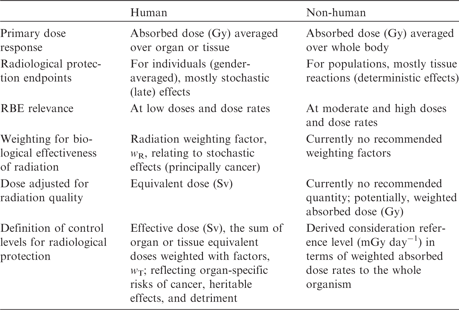
(5) The current ICRP dosimetric approach for non-human biota uses the concept of absorbed dose (i.e. the mean radiation energy absorbed per unit mass of matter). The main dosimetric quantities, primarily as DCs, are correspondingly defined in terms of absorbed dose. (6) The effects of radiation on living tissues are known to depend on the type and energy of radiation or, more precisely, on the density of ionisation produced by the radiation in tissue, which is expressed by the linear energy transfer. These effects are accounted for in human radiological protection dosimetry by introducing the concept of equivalent dose. The latter is calculated from absorbed dose using radiation weighting factors (wR) that numerically express radiation quality with respect to specific protection endpoints (ICRP, 2003b, 2007). Radiological protection endpoints for animals and plants (ICRP, 2014a) differ from those for humans; nevertheless, a similar concept of wR can be adopted for non-human biota (Table 2.1). Numerical values of wR for various non-human organisms are subject to discussion, and ICRP has not made recommendations on this topic to date; however, others (e.g. UNSCEAR, 2008; Higley et al., 2012) have published values. To facilitate the possible application of wR to the DCs presented in Annex B of the present publication, fractions of the total dose due to different radiation types are provided separately. These radiation types are: (a) spontaneous fission fragments and alpha-recoil nuclei; (b) alpha particles; (c) low-energy (Eβ <10 keV) electrons and photons; and (d) higher-energy electrons and photons. Thus, weighted dose can be readily computed as a product of the DCs and the sum of the radiation fractions weighted with the values of the adopted wR. (7) Assessment of exposures of non-human biota in their natural environments can be a more complicated task than dosimetry for humans, because of the wider variability and vast diversity of non-human biota and of their exposure conditions. It is also necessary to consider possible risks of importance in relation to exposures of non-human species, namely risks of population depletion. Consequently, the aim is to develop and use simple but plausible and robust models to deal with the diversity of environmental exposures of non-human biota. For example, only simplified shapes are used to describe the body of an organism, and no account is taken of their internal structures or organs. Additionally, metabolism and the biokinetic behaviour of radionuclides within organisms are not considered. The calculated DCs are defined per unit average concentration of radionuclides in the body or in the surrounding media. Such definitions imply assumptions of uniform distribution of radioactivity throughout the body and in the surrounding environment. (8) Assessment of internal doses requires knowledge of DCs and activity concentrations in the organisms’ bodies. The latter is often unknown but is estimated using empirically defined transfer factors, or by modelling transfer of radioactive materials in the environment and intake by the organisms of concern. Uncertainties of such model estimates can be high, and significantly exceed those inherent to DCs. Comparison of dosimetric quantities underlying the ICRP systems of radiological protection of human and non-human biota. RBE, relative biological effectiveness.
3. ICRP DOSIMETRIC SYSTEM FOR NON-HUMAN BIOTA
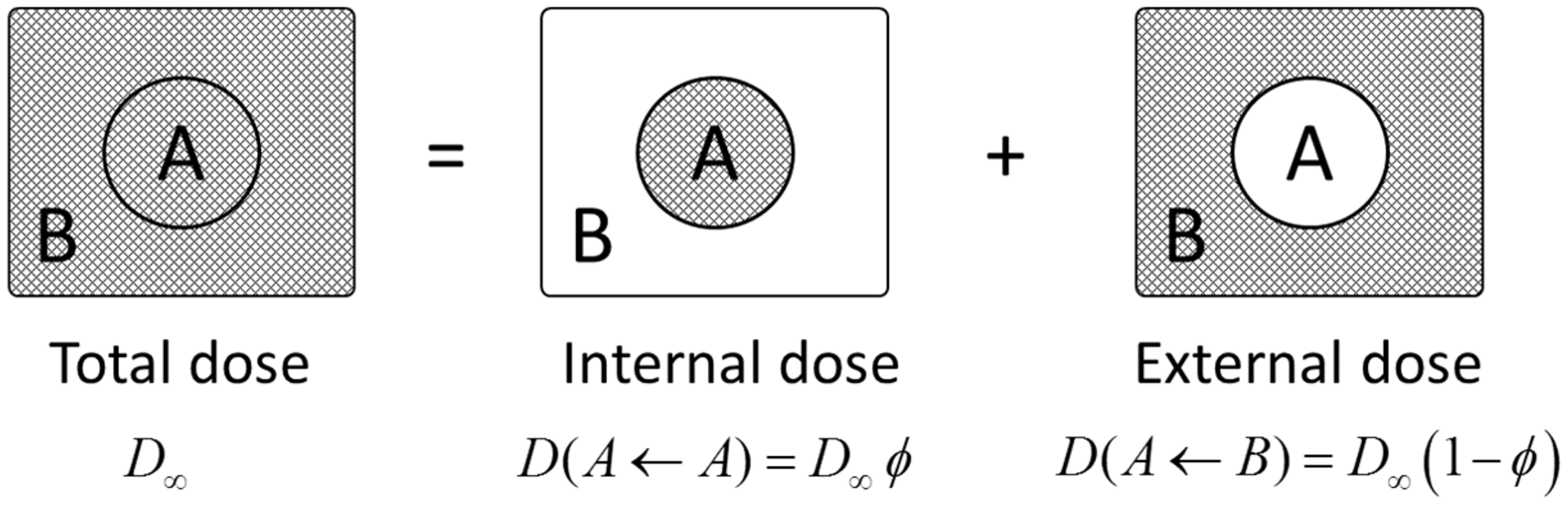
(9) The dosimetric approach adopted by ICRP and presented in Publication 108 (2008b) is, to a large extent, built around the uniform isotropic model introduced by Loevinger and Berman (1968, 1976). The model represents the organism and its environment as an infinite homogeneous medium uniformly filled by isotropic radiation sources. The model can be applied if the density and elemental composition of the organism’s tissues are close to that of water, and if the distribution of radioactivity in the organism’s body or in the surrounding environment can be assumed to be uniform. Aquatic organisms closely match the conditions of this uniform isotropic model, and thus the model naturally appears as a plausible choice for modelling radiation exposures of aquatic biota. (10) Under the assumptions of the uniform isotropic model, the dose rate per unit activity concentration remains the same in every point of the medium, and is equal to the ‘full absorption limit’, which is numerically expressed as the total energy emitted by the radiation source per single event of radioactive decay (nuclear transformation):
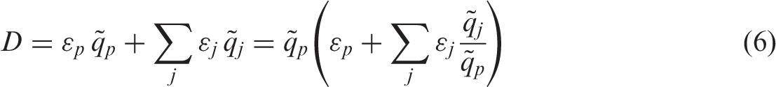
(11) Within the framework of the uniform isotropic model, DCs for internal and external exposures can be expressed as fractions of the ‘full absorption limit’ value (Fig. 3.1). DCs for internal exposure, Uniform isotropic model: the total dose for organism A in medium B is represented as a sum of doses from internal and external sources. Equations shown are for mono-energetic radiation. Source: Ulanovsky and Pröhl (2012). (12) Provided that radionuclide emission data are available, DC calculation for aquatic biota requires only knowledge of the AF for radiation of various types and energies, and for bodies of various shapes and masses. Short-range radiations (alpha particles, alpha-recoil nuclei, and spontaneous fission fragments) can be regarded as non-penetrating, and all their energy is assumed to be deposited locally. In terms of the adopted approach, for all practical purposes, AFs for these radiation types are equal to 1. (13) AFs for penetrating radiation (photons and electrons) have been assessed based on systematically calculated energy-dependent AFs for simple spherical and ellipsoidal bodies surrounded by infinite water medium (Ulanovsky and Pröhl, 2006). The calculated photon and electron AFs were found to be smooth functions of particle energy and the mass of the organism’s body; thus, AFs for other masses and energies could be easily derived by interpolation from the data provided. (14) To facilitate interpolation of the AFs between different shapes, an analytical approximation was suggested (Ulanovsky and Pröhl, 2006), which provided a method for the transformation of AFs for spheres to those for arbitrary ellipsoidal bodies by means of a scaling factor. The scaling factor is a function of a ‘non-sphericity parameter’ η, which expresses the degree of deviation from sphericity for the given ellipsoidal shape. The parameter η is a quotient of the surface area of a sphere (S0) and that of an ellipsoid (S) of equal volume (mass). Thus, for spheres, the parameter value is equal to 1, whereas for non-spherical bodies, it varies between 0 and 1. The closer the parameter to 0, the more the shape of the body deviates from a sphere. A value of 0 for the parameter corresponds to an infinitesimally thin line or plane. (15) The analytical approximation allows the calculation of photon and electron AFs for organisms with body masses in the range from 1 mg to 1000 kg, and with body shapes from spherical (η = 1) to highly protracted or oblate ellipsoids (η = 0.15). The uncertainty of the approximation (expressed by absolute coefficient of variation) was shown not to exceed 15% for photons and 10% for electrons (Ulanovsky and Pröhl, 2006). Although the analytical approximation is defined for the above body mass range, a technique can be used to extrapolate DCs to mass values beyond this range. Such extrapolation exploits the fact that within the uniform isotropic model, neither external nor internal dose can exceed the ‘full absorption limit’. Details and justification of the extrapolation technique can be found in Ulanovsky and Pröhl (2006). (16) Amato et al. (2009, 2011, 2013) and Amato and Italiano (2014) recently reported alternative analytical approximations for AFs of gamma, beta, and alpha radiations in ellipsoidal bodies. These approximations, being practical and computationally convenient, were developed for a limited set of ellipsoidal bodies and radionuclide sources, thus their applicability needs investigation; thorough comparison with the approach adopted in Publication 108 (2008b) and in the present publication appears to be necessary. (17) Being originally developed for internal and external exposures of aquatic organisms, the analytical approximation of AFs for non-spherical bodies was applied to calculation of DCs for internal exposure of terrestrial animals and plants (Ulanovsky and Pröhl, 2008; Ulanovsky et al., 2008). AFs for aquatic organisms are somewhat higher than those for similar terrestrial organisms because of the effect of secondary radiation scattered back from water medium surrounding an aquatic organism. However, in most practical cases, the effect of backscattered radiation can be safely neglected. For example, calculation by Monte Carlo methods of DCs for a spherical organism with a mass of 1 mg in water and in air has shown that the overall contribution of the backscattered radiation is 6% for 1.5-MeV photons and less than 1% for 0.15-MeV photons (Ulanovsky and Pröhl, 2008). (18) In most cases, external exposure of terrestrial animals and plants cannot be modelled using the uniform isotropic model; thus, the DCs for external exposure of terrestrial animals were mainly based on results of various ad-hoc models, primarily those developed in the framework of the FASSET project (Taranenko et al., 2004). For example, using a set of predefined terrestrial organisms with body masses varying from 0.17 g to 550 kg, DCs have been computed for mono-energetic photon sources in soil. Two types of source distribution in soil were considered: planar at a depth of 0.5 g cm−2, and uniform volume distribution in the upper 10 cm of soil. Additionally, exposure of burrowing animals with masses from 0.17 g to 6.6 kg was estimated for location in the middle of 50-cm-thick source in the upper soil. External exposure of vegetation was estimated using simple models of infinite homogeneous layers of different thicknesses parallel to the ground, representing grasses, shrubs, and trees. (19) It was recognised that external exposure of terrestrial animals and plants was not addressed adequately by the previous ICRP dosimetric methodology, which considered a narrower range of body masses than that for aquatic organisms, a limited set of environmental sources, and provided a very limited set of DCs for organisms located not on the ground surface but at various heights above. Therefore, systematic extension of the dataset necessary for estimation of the external exposures of terrestrial organisms appeared among the priority tasks in the extension and improvement of the existing methodology.


4. EXTENSION OF THE EXISTING ICRP DOSIMETRIC SYSTEM
4.1. Ranges of applicability
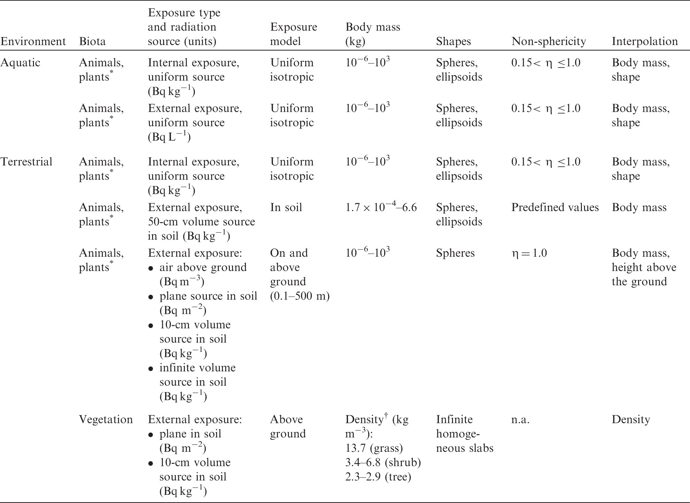
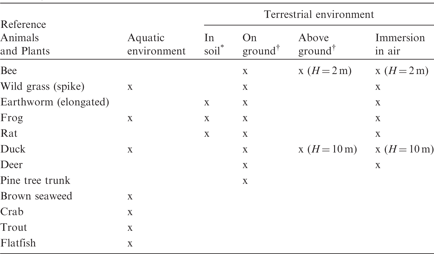
(20) The extended dosimetric system presented in this publication improves compatibility between the treatment of internal and external exposure of terrestrial organisms by providing DCs for the same range of body masses: from 1 mg to 1000 kg. Also, two new sources of external exposure of terrestrial organisms are added: infinitely deep uniform source in soil, and uniformly contaminated air above the ground surface. Forms of biota, body masses and shapes, types of exposure, and radiation sources considered in the current dosimetric system are shown in Table 4.1. Types of organisms, exposure conditions, and dosimetric models represented in the current dosimetric methodology for non-human biota. n.a., not applicable. Ignoring minor effects due to different chemical composition of tissue. Density of homogeneous mixture of biomass and air.
4.2. Radionuclide emission data
(21) Publication 107 (ICRP, 2008a) replaced Publication 38 (ICRP, 1983) with an updated and significantly extended dataset, considering radiation emitted due to decay of 1252 radioactive isotopes of 97 elements. New DCs presented here have been recalculated using the radionuclide emission data of Publication 107, and may therefore differ from the values given in Publication 108 (ICRP, 2008b). The transition to the new database also necessitated the calculation of new photon and electron AFs up to 10 MeV to address maximum emitted energy for some additional radionuclides. As with the previous data from Publication 38, numerical integration of continuous beta spectra is used in the DC calculation, thus accounting for different ranges of electrons of various energies in the same emission spectrum (Eckerman et al., 1994).
4.3. Models for external exposure
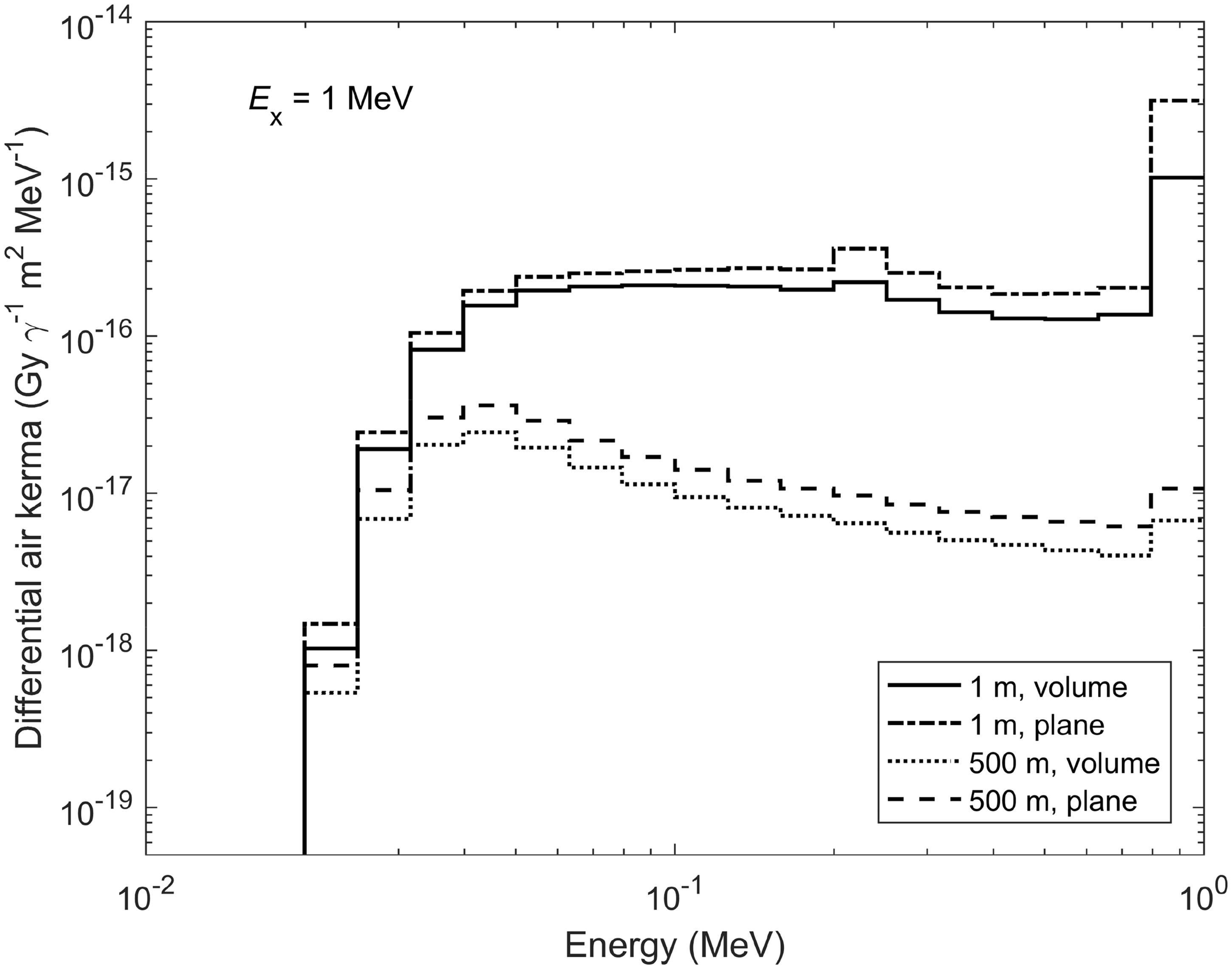
(22) For aquatic organisms, external exposure is treated under the assumptions of the uniform isotropic model, enabling both internal and external DCs to be assessed coherently by the same method and within the limits imposed on a body’s mass and shape. The simplest geometry of an infinite medium is adequate for aquatic biota in water. Exposure of aquatic biota at the interface between water and sediment can be easily reduced to a simple exposure geometry by applying the superposition principle and accounting for the similar density of water (1000 kg m−3) and underwater sediment (typically, around 1500 kg m−3). (23) Estimating DCs for external exposure of terrestrial animals and plants is a more complicated and laborious task. This is because of the considerable variations in exposure geometry; composition and densities of soil, air, and organic matter in terrestrial environments. External exposure scenarios cannot, in general, be adequately taken into account by the uniform isotropic model. (24) Current DCs for external exposure of terrestrial organisms are based on results obtained by Monte Carlo simulation of radiation transport in terrestrial environments (Taranenko et al., 2004; Ulanovsky, 2014), where only external exposure to photons was considered. Any contributions from alpha particles and electrons to external doses to terrestrial organisms were neglected because of their short range, and due to the fact that radiosensitive tissues are usually covered by inert layers (e.g. dead skin, fur, feather, shell, or bark), thus being located beyond the reach of low-penetrating radiation. Although the current approach can be considered reasonable in many practical external exposure situations for terrestrial biota, there may also be scenarios involving exposure to secondary bremsstrahlung photons from pure beta-emitting sources (e.g. 90Sr) or exposure of small organisms located closely to radioactive sources emitting high-energy electrons where this approach becomes inapplicable. Exposure of terrestrial biota to bremsstrahlung radiation is not covered by the current approach, so the former exposure situation cannot be addressed using the DCs available in this publication (see Annex B), while for the latter situation – exposure of a small organism on or close to the ground surface – a surrogate conservative estimate can be derived using the DCs for aquatic organisms, where contributions from external electron sources to exposure of skinless organisms are accounted for, and applying geometric factor 0.5. (25) Due to the complexity of the processes involved and the variation between terrestrial life forms, all possible exposure conditions cannot be addressed. Generalised representative cases as defined by source configuration and energy, contaminated media, organism sizes, and source/target relative locations have therefore been selected for detailed consideration. DCs for any intermediate exposure configurations for which detailed calculations have not been made can then be deduced by interpolation between the calculated DCs. Here, the following source-target scenarios are considered (also see Table 4.1): External exposure of in-soil RAPs situated in the middle of a uniformly contaminated volume radionuclide source with a thickness of 50 cm. External exposure of animals and plants on and above the ground surface due to a planar radionuclide source at a depth of 0.5 g cm−2 in the soil, which can be regarded as representative of radioactivity freshly deposited on the ground, accounting for surface roughness and initial migration (Jacob and Paretzke, 1986). External exposure of animals and plants on and above the ground surface due to a uniformly contaminated volume radionuclide source within soil with a thickness of 10 cm, which can be treated as representative of aged contamination of soil following substantial downward migration and activity redistribution. External exposure of animals and plants on and above the ground surface due to an infinitely deep radioactive source in soil, which can be regarded as a source representative of naturally occurring radionuclides or anthropogenic contamination of the environment strongly affected by downward migration, agriculture, or decontamination practices. External exposure of animals and plants located on and above the ground surface due to immersion in air contaminated with radioactive materials. (26) With the exception of in-soil exposure, all other scenarios have been re-assessed systematically using the new approach (Ulanovsky, 2014). In the adopted approach, whole-body doses arising from external exposure above the ground surface due to various photon sources in soil or in the ambient air can be estimated for arbitrary heights above the ground surface up to 500 m, and for any organisms with body masses from 1 mg to 1000 kg. Such flexibility is possible due to the factorisation of the external dose into free-in-air kerma spectrum and energy-dependent ratios of whole-body absorbed dose and air kerma. (27) The free-in-air kerma Kair (ICRU, 2011) at height H above radioactively contaminated terrain with photon sources of energy Ex can be expressed as the integral of the mass-energy transfer factor for the specific differential photon fluence (spectrum) as follows:
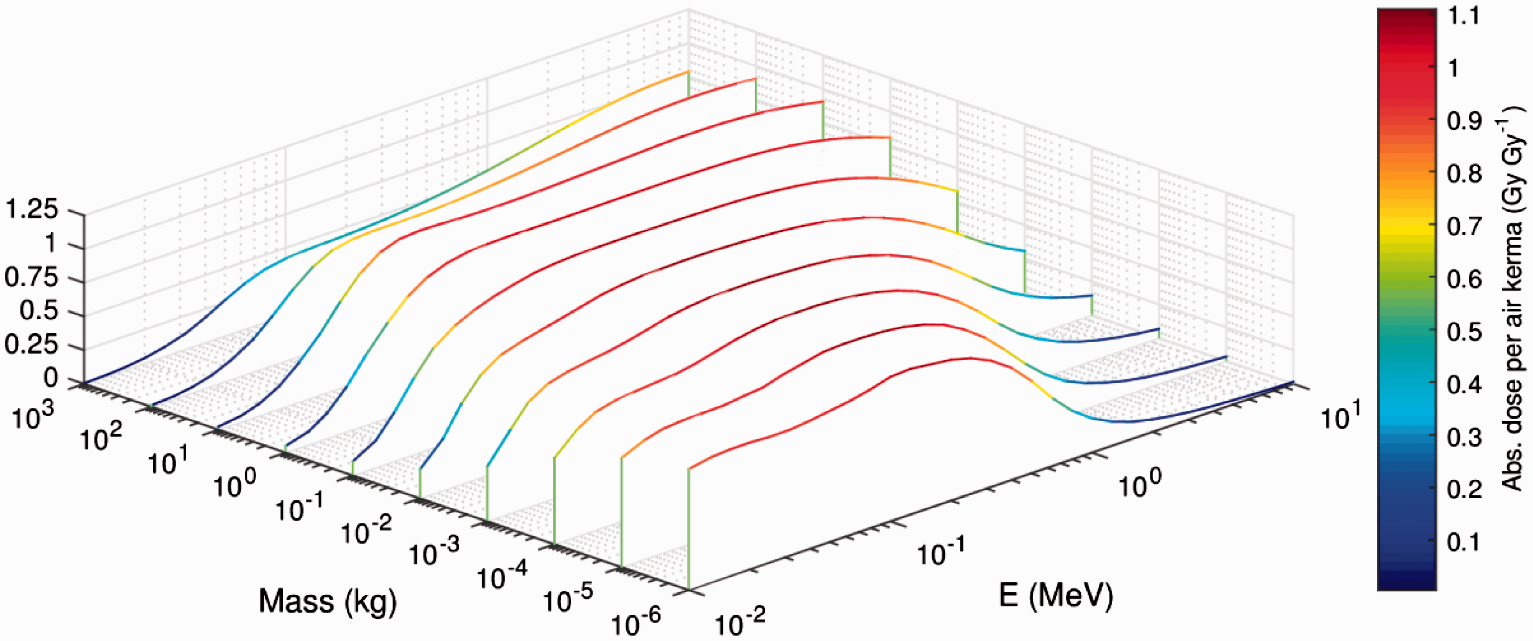
(28) The differential air kerma is known to depend on the geometry of the terrain and source distribution, distance between the source and the target biological receptor, soil density, chemical composition and water content of the soil, and physical properties of ambient air (Beck and de Planque, 1968; Jacob and Paretzke, 1986; Eckerman and Ryman, 1993; ICRU, 1994). Due to this dependence on multiple factors, Monte Carlo simulation of radiation transport in the environment is the only practical method for assessing the kerma spectra. Correspondingly, the kerma spectra were calculated for the sources detailed above in an idealised infinite terrain with homogeneous soil and plane ground interface (Ulanovsky, 2014). An example of the differential air kerma for two photon sources in soil, namely, planar at a depth of 0.5 g cm−2 and volume in the upper 10-cm-thick layer, at heights above the ground surface of 1 and 500 m, is given in Fig. 4.1, where the kerma spectra are shown in group representation for 1-MeV source photons. (29) Absorbed dose (per source particle) in an organism with body mass M located above contaminated soil or immersed in contaminated ambient air can be expressed via the differential air kerma at the same location and organism-specific energy-dependent dose response:
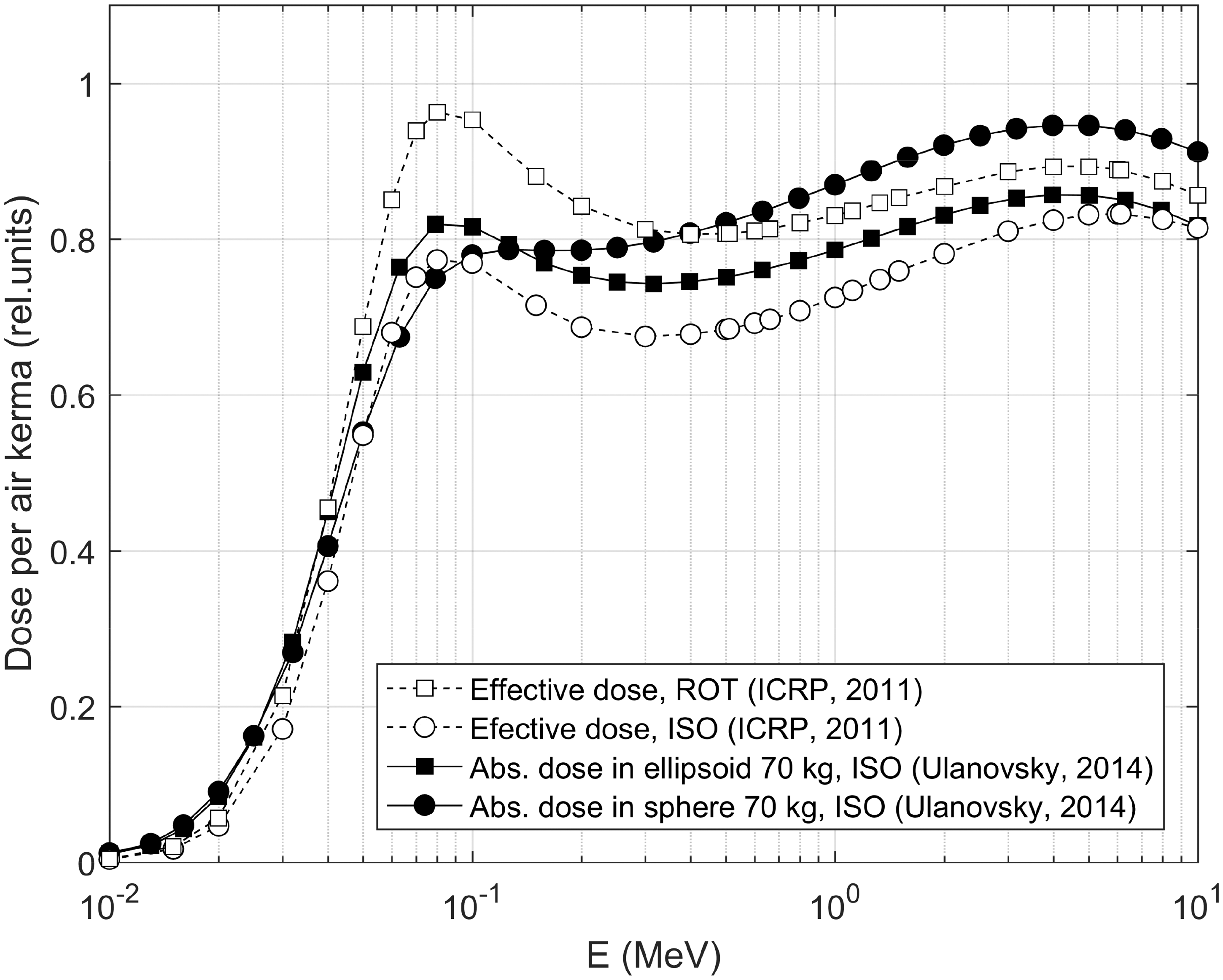
(30) The conversion factor R(E,M) generally depends on the energy and angular distribution of incident photon fluence as well as on the mass and geometric shape of the organism. When the dosimetric endpoint is the average absorbed dose in the whole body, the subtle effects of anisotropic angular dependence in the dose response can be neglected, and angular-integrated kerma spectra can be used. Correspondingly, biota above the ground surface can be modelled as tissue-equivalent spheres, and their dose response per air kerma can be computed for isotropic photon fields. (31) An example of the response R(E,M) is given in Fig. 4.2, where ratios of average whole-body absorbed dose and air kerma are shown as computed for tissue-equivalent spheres with masses from 1 mg to 1000 kg located in an isotropic field of mono-energetic photons with energies ranging from 10 keV to 10 MeV (Ulanovsky, 2014). It can be seen from Fig. 4.2 that the strong attenuation of low-energy photons in massive bodies leads to a reduction of the average absorbed dose when compared with free-in-air kerma. This is the case of ‘opaque’ bodies, which are ‘non-transparent’ to the specific radiation. A similar reduction of absorbed dose can be observed in the opposite case of low body masses and high energies of source photons; this is the case for bodies ‘transparent’ to radiation of the given energy. It is also worth noting that in the range of source energies from approximately 20 keV to 2 MeV, and for bodies with masses from approximately 1 g to 100 kg, the absorbed dose-to-air kerma ratio does not vary much, showing values between 0.8 and 1.15, thus indicating that, for the given conditions, there may be negligible differences in absorbed dose in the whole body from air kerma, such that air kerma can serve as a reasonable surrogate for the average whole-body absorbed dose. (32) Use of spherical shapes for modelling bodies of various organisms that would be better represented by non-spherical shapes introduces some uncertainties in modelled DCs, and reduces their applicability as an assessment of average absorbed dose in the whole body. Realistic representation of the body shape and its internal structure as well as irradiation geometry might be important when dosimetric endpoints are absorbed doses in particular organs, or exposure conditions suggest highly anisotropic irradiation of a static or slowly moving organism. However, if the study endpoint is the average absorbed dose in the whole body of an agile organism exposed in highly variable environmental conditions, then the absorbed dose-per-air kerma coefficients for simple spheres can be regarded as a reasonable approximation. An example is shown in Fig. 4.3, where absorbed dose-per-air kerma values for a 70-kg sphere (closed circles) and for a 70-kg ellipsoid with extensions 167.2 × 40 × 20 cm (closed squares) are compared with effective dose-per-kerma values from Publication 116 (ICRP, 2010b) for rotational and isotropic fields (open squares and circles, respectively). All response curves in the figure are remarkably similar, and the effect of non-spherical body shape on the dose–kerma ratio R(E,M) is small. (33) Some of the earlier simpler models (Taranenko et al., 2004) are still used for the present tabulation of external exposure DCs for terrestrial plants. These models represent plants as uniform mixtures of biomass and air in the form of slabs placed above the ground. Grass is represented by a 10-cm-thick layer with density of 13.7 kg m−3, bushes and shrubs are described by a 90-cm-thick layer of density in the range 3.4–6.8 kg m−3 over the grass layer, and trees are modelled as a 9-m-thick layer of density in the range 2.3–2.9 kg m−3 over the shrub layer. Such simple models may be inadequate for some specific assessments (e.g. when looking for realistic distribution of external doses in single plants or to external exposures from radioactive sources in air or distributed in soil depth). These DCs are given for only two types of radioactive sources in soil: planar at depth 0.5 g cm−2 and 10-cm-thick volume. (34) The DCs for external exposures of terrestrial animals and plants were calculated for photon-emitting sources alone, neglecting exposures to secondary photon radiation (bremsstrahlung) produced by electrons decelerating in matter. Effects of bremsstrahlung are generally weak and can be considered as corrections of a lower order to the dose estimates in many practical dose assessment tasks. However, external exposure in environments highly contaminated by pure beta emitters, such as 90Sr or 32P, could be mostly due to penetrating secondary photon radiation. Such situations should be considered as non-standard and not covered within the framework of the currently adopted dosimetric approach, thus requiring special considerations and, possibly, development of new non-standard dose assessment techniques. Differential air kerma (kerma spectra) for planar at depth 0.5 g cm−2 and 10-cm-thick volume sources in soil at heights 1 and 500 m above the ground surface [based on data from Ulanovsky (2014)]. Average absorbed dose per air kerma conversion factor (Gy Gy−1) for tissue-equivalent spheres of various masses in an isotropic field of mono-energetic photons [based on data from Ulanovsky (2014)]. Comparison of dose-per-kerma ratios (Gy Gy−1) for a tissue-equivalent 70-kg sphere and a 70-kg ellipsoid in an isotropic field of mono-energetic photons (Ulanovsky, 2014) with effective dose per air kerma (Sv Gy−1) for an adult human in rotational (ROT) and isotropic (ISO) external photon fields (ICRP, 2010b).


4.4. Contribution of radioactive progeny to dose coefficients
(35) Decay products of many radionuclides are themselves radioactive and may contribute to radiation exposure. The contribution of radioactive progeny to radiation exposure of non-human biota is commonly attributed to the parent radionuclide, subject to various assumptions. The most common approach is a simple and pragmatic method in which only part of the full decay chain is taken into account, assuming full equilibrium between the parent radionuclide and its progeny. Criteria for truncation of decay chains are commonly based on selection of an upper limit for physical half-life of a daughter to be accounted for in the given chain. Selection of the upper limit varies in the literature, with values of 1 day (Amiro, 1997), 30 days (Jones, 2000; DOE, 2002), 180 days (Yu et al., 1993), and 100 years (Higley et al., 2003). The approach adopted in Publication 108 (ICRP, 2008b) was to apply a chain cut-off criterion of 10 days, as in the FASSET and ERICA projects (Larsson, 2004, 2008) and in the ERICA tool (Brown et al., 2008). Additionally, within the ERICA tool and the ICRP approach, the chain is cut at a daughter nuclide if its physical half-life is longer than that of the parent, because in such case, the parent and the daughter would never reach equilibrium. (36) Truncation of decay chains based on criteria of maximum allowed physical half-life of a daughter is a simple and pragmatic solution when dealing with a limited set of radionuclides of immediate practical importance for a specific assessment. However, depending on the assessment task, the chain truncation criteria may vary and need to be modified accordingly. Moreover, development of software tools for DC calculation, which use a comprehensive database of radionuclides, also requires the introduction of an accurate and flexible method for accounting for radioactive progeny. Even more importantly, it should be recognised that the method of cutting a decay chain and assigning equilibrium activity ratios to chain members implicitly assumes that the decay chain is linear, and the method may lead to ambiguous results when applied to complex, branching, and merging decay chains. (37) More robust and flexible approaches, capable of addressing different exposure scenarios, can be formulated using weighting factors for the members of decay chains based on their time-integrated activities. Accounting for radioactive decay alone (i.e. implying long retention in the organism relative to radioactive decay in the case of internal exposure or no migration of radioactivity deposited in the environment), one can express the dose as follows:
(38) Such an approach implemented within software tools for DC calculation can account for the contribution of radioactive progeny for all types of radioactive decay chains by numerical integration of the differential equations describing the decay chain. Correspondingly, the integration time can be selected to be pertinent to the specific assessment task (e.g. based on the lifetime and behaviour of the organism of concern, exposure conditions in its habitat, and temporal changes in radioactive contamination of the environment). An example of such an approach was provided by Ulanovsky (2014), where DCs for external exposure of terrestrial biota were computed for different averaging times depending on the environmental source: 15 days for a freshly deposited (planar) source in soil, 1 year for an aged (10-cm-thick volume) source in soil, and an infinite time (secular equilibrium ratios) for natural radionuclides uniformly distributed in the soil depth. For computation of DCs accounting for ingrowth of radioactive progeny within given time intervals, the special software tool can be used (see below).
4.5 Dose coefficient tables and software tool BiotaDC
(39) This publication is complemented by tables of DCs for RAPs (Annex B). The tables are given for the same list of radionuclides as in Publication 108 (ICRP, 2008b), but have been recalculated using the new radiation emission dataset from Publication 107 (ICRP, 2008a). Another distinctive feature of the new tables is their organisation and layout, which differ substantially from those used in Publication 108. The present tables are organised to present data on individual radionuclides, making it easier to identify interspecies and intersource differences. As can be seen from the DC tables (Annex B), in many cases, such differences can be regarded as insignificant or low, indicating that DCs are not among the main contributors to assessed uncertainties for exposure scenarios in these cases, and that attention should be focused on other, probably more significant, sources of uncertainty in the estimated doses. (40) The current tables include DCs for external exposure of terrestrial animals and plants on and above the ground surface for radioactive sources in the upper 10 cm of soil and in the ambient air. Additionally, DCs are given for exposure of small animals (earthworm, frog, and mouse) in the soil. DCs for planar or infinitely deep sources in soil are not shown in the printed tables, but they can be derived easily using the software tool BiotaDC (see Annex C). Similarly, DCs for flying organisms (bee, bird) are presented only for two exemplary values of flight height, and the coefficients for other conditions, characterised by flight height and mass of the organism, can be derived using the software tool. Table 4.2 shows the external exposure conditions considered in the published version of the DC tables. (41) To facilitate compatibility with previously published data, the DC tables are calculated here using the same criterion to account for the effect of radioactive progeny as in Publication 108 (2008b) (i.e. the decay chain is truncated at the first daughter nuclide with physical half-life of >10 days, or longer than that of the parent nuclide). Activity ratios between the parent radionuclide and progeny are calculated assuming secular equilibrium conditions. (42) In Publication 108 (2008b), DCs were given for adult forms of RAPs and for RAPs at various developmental stages (eggs, mass, larvae, etc). The tabulation presented here shows DCs for adult forms of RAPs alone, for two reasons. First, as seen from the DC tables in Annex B, variability between DCs for many radionuclides can be regarded as insignificant and ignored, or differences resulting from the mass changes of one organism during development can be determined relatively easily by simple interpolation of the values shown for other RAPs. Second, the software tool BiotaDC (Annex C) is introduced with this publication and can be used to generate DCs ‘on demand’ by means of a fully flexible user-friendly interface, accounting for non-standard (user-defined) organisms of specific shapes and body masses, and under various exposure conditions, including different methods of accounting for the contribution from radioactive progeny. (43) The current dosimetric system for non-human biota is built assuming uniform distribution of radioactivity in a homogeneous ‘skeleton-less’ body. Although in many practically relevant cases, these assumptions are reasonable and corresponding uncertainties in DCs are much less than those for other parameters important for dose assessment (see e.g. Gómez-Ros et al., 2008), there may be situations when the non-uniformity of activity distribution in the body becomes an important consideration in dose calculations. In such situations, simple scaling techniques can be used, as suggested in Publication 108 (ICRP, 2008b). (44) Additionally, assessment of internal doses to organs can be performed using known radionuclide activity in the organ and its mass, and applying the assumptions of the uniform isotropic model. Specifically, this can be achieved by replacing the body of the whole organism with an artificial ‘body’ with the size and mass of the organ of interest. These tasks can be readily achieved by interpolating DCs using the published tables, or by direct calculation using the software tool BiotaDC (Annex C). (45) Radiation exposure due to inhalation of radioactively contaminated air is not considered explicitly in the current dosimetric approach, as it would require organism-specific biokinetic data and models. Simplified methods can be applied to assess inhalation doses conservatively using allometric scaling. (46) Allometric relationships appear as powerful tools in dealing with biota diversity. They numerically express similarities and common properties between various organisms. Recent studies (e.g. Kolokotrones et al., 2010) demonstrated that allometric relationships in the form of power law do not always describe biological properties of animals and plants satisfactorily. A concept of generalised allometric relationship was therefore suggested (Ulanovsky, 2016), and generalised allometric equations have been shown for breathing and basal metabolic rates of mammals (Annex A). (47) In comparison with Publication 108 (ICRP, 2008b) and the ERICA tool (Brown et al., 2008), the current methodology for assessment of external exposure DCs for terrestrial animals and plants has been systematically expanded and improved in the present publication. Further development might allow for a wider range of irradiation geometries and sources, or account for different shapes of organisms’ bodies by interpolation techniques. Estimates of organ doses due to external exposure may be required. Summary of external exposure scenarios included in the dose coefficient tables (see Annex B). Organism exposed in the middle of a 50-cm-thick uniform volume source in soil. Organism exposed on or above a 10-cm-thick uniform volume source in soil.
5. UTILISATION OF DOSE COEFFICIENTS IN EXPOSURE ASSESSMENT
(48) This publication describes methods and presents a set of DCs for animals and plants. DCs are essential for environmental dose assessments. It is often the case in practical assessments that uncertainties in DCs are small compared with other sources of uncertainty. Such uncertainties can originate from variability of environmental contamination, lifestyle, time spent by organisms in various habitats, and other factors. In this section, the basic principles of dose assessment are reviewed to indicate the place of DCs within an assessment framework, to emphasise simplifying assumptions, and to identify other essential components of the assessment. (49) Radiological protection of non-human biota is formulated for biological endpoints at the level of populations (ICRP, 2014a), and it can thus be regarded as focusing on tissue reactions of radiation on populations, whereas human radiological protection requires the prevention of tissue reactions and minimisation of stochastic effects (ICRP, 2007). From a dosimetric viewpoint, the consideration of average whole-body dose in animals and plants as appropriate for the objectives of environmental radiological protection is a pragmatic decision. It may be that further analysis of possible tissue reactions may require consideration of organ doses under particular circumstances of exposure. In the protection system for humans (ICRP, 2007), limits are set on organ doses to prevent tissue reactions, while the limitation of stochastic effects employs the protection quantity, effective dose, which sums organ doses according to their contribution to overall stochastic risk (mainly cancer). (50) For internal exposure, the dose, D (Gy), from radioactivity incorporated in the whole body and acquired during period ΔT can be written as follows:
(51) The time dependence of DCs is due to temporal changes of the organism during the exposure time (e.g. growth or transformations), and also due to time-dependent activity ratios of the parent radionuclide and its radioactive progeny in a non-equilibrated decay chain. While the changes related to an organism’s growth are generally ignored, changes due to transformations can be addressed by considering the organism at various developmental stages as different species. The latter, for example, was done in Publication 108 (ICRP, 2008b) where the adult forms of RAPs were supplemented by organism forms at various developmental stages (egg, egg mass, larvae, tadpole). The time dependence of DCs due to changes in activity ratios of the parent radionuclide and its radioactive progeny should also be considered; for example, in the case of environmental contamination by 241Pu, in-growth of the daughter 241Am should be considered for organisms with lifetimes of several years or more. As shown in Section 4.4, the contribution of radioactive progeny can be adequately taken into account by selecting appropriate time periods for the calculation of time-integrated activity ratios between the parent and daughter nuclides. The selection of integration times should be conditional on characteristics of the specific assessment task, including the contamination scenario, biota of concern, behaviour, etc. (52) Eq. (7) represents dose as the integral of the product of two time-dependent quantities: DC and the activity concentration in the organism. Provided the temporal changes in DCs are small, the equation can be factorised and shown in a simpler form:
(53) As seen from Eq. (7), another essential part of the dose assessment is an estimate of the time-dependent activity concentration in the whole body. If the activity concentration of the radionuclide is not measured, it has to be estimated. Such estimation can become a challenging task. A widely used approach utilises concentration ratios (CRs), which are commonly applied to derive activity concentrations in the (whole) organism from activity concentration in the surrounding environment. Publication 114 (ICRP, 2009) has summarised the available data on CRs for non-human biota found in the literature, and presented evaluated data along with assessed uncertainties. However, estimates of CRs for many elements are missing or incomplete, while available CRs, being parameters that implicitly include many processes assuming equilibrium, often show considerable uncertainties. Inherent uncertainties of CRs are mostly due to individual and environmental variability and non-equilibrium conditions. The latter source of uncertainty is due to the definition of CRs as an equilibrium constant CR between the biota and the surrounding environment. (54) Non-equilibrium CRs can be expressed as the quotient of the time-dependent activity concentrations in the organism and that in the environment (water, soil, air). Environmental contamination can be highly variable in space and time. Provided that the activity concentration in the environment and intake pathways are known, the activity concentration in the organism’s body could, in principle, be assessed using biokinetic modelling. However, this approach requires biokinetic data for individual radionuclides, as well as physiological and anatomical data. Even a simple, single-compartmental, kinetic model is represented by a convolution integral between so-called ‘intake’ and ‘retention’ functions:
(55) Use of CRs is a very approximate way to assess activity concentration in the whole organism, and uncertainty is generally high. Gathering and systematisation of information on biokinetic behaviour of radionuclides in animals and plants would lead to more flexible and realistic dosimetric models. Some models are already available, opening the possibility of time-dependent assessment under non-equilibrium conditions, such as those following the Fukushima accident (Kryshev et al., 2012; Vives i Batlle et al., 2014). (56) The whole-body dose from external exposure, D (Gy), acquired by the organism during the period ΔT can be represented as follows:
(57) The life history of the organism, time fraction spent by an organism in various parts of the heterogeneous environment, distributions of radioactive contamination, and radionuclide composition of the contamination can be complicated and time-dependent. Such complicated exposure scenarios have to be represented by superposition of simpler scenarios. If occupancy fractions are not known, they have to be implied or derived from biological data. Data on contamination of the environment in specific locations may have considerable uncertainty originating from various sources, including spatial variability of the environmental contamination, scarcity of measured data (e.g. sampling is performed in certain locations, not in the whole area), or use of radionuclide dispersion and/or radio-ecological transfer modelling in cases where there are no measurement data. (58) This publication does not address exposure from radon isotopes, which may contribute significantly to exposure of biota, either from natural or anthropogenic-enhanced sources, for some organisms and some environments. Assessing doses of radiation exposure due to radon isotopes and their progeny commonly appears as a difficult task due to complicated processes of radon effluence, build-up of radioactive progeny, transport in air, chemical forms and attachment to aerosols, intake, and deposition and retention of radon-related radioactivity in the body of living organisms. For humans, standard biokinetic and dosimetric models have been developed to derive dose coefficients for radon exposure (ICRP, 2010a). The diversity of non-human biota, expressed by their biological, morphological, and metabolic differences, makes radon dosimetry for biota a substantially more complicated task than for humans; as such, in this case, the use of simplified and conservative methods (models) appears to be rational and appropriate.


REFERENCES
ANNEX A. GENERALISED ALLOMETRIC RELATIONSHIPS
(A1) As stated in Section 5 of the main publication, DCs are not the only essential parts of any dose assessment. Assessing doses from internal exposure needs not only DCs but also estimates of body burden by radioactive materials; the latter to be estimated either via aggregated transfer factors (CRs), or by evaluating intake and retention in the body using biokinetic compartmental models. Variability of living organisms makes biokinetic modelling a challenging task; therefore, biologically and physically plausible inter- and extrapolations are considered as important instruments to account for the diversity of biota. Included in this annex are generalised allometric parameterisations for basal metabolic and inhalation rates of terrestrial mammals. Unlike conventional allometric relationships (e.g. Whicker and Schultz, 1982), the generalised allometric relationships represent a novel concept that accounts for non-linear effects in the observed biokinetic data, and also quantifies uncertainties of the data due to interspecies variability. (A2) Despite extreme variability, living organisms display similarities of certain basic characteristics. So-called ‘allometric laws’ can be used to express such similarities within groups of living organisms (e.g. mammals, insects, warm- or cold-blooded species). Allometric models relate quantitative parameters, such as breathing rates or metabolic rates, to the mass of their bodies. Originating from findings made in the late 19th century (Rubner, 1883) and based on the so-called ‘Kleiber law’ (Kleiber, 1947), allometry has also been the subject of more recent studies (e.g. Marquet et al., 2005; Nagy, 2005; West and Brown, 2005; White and Seymour, 2005). (A3) Allometric relationships are commonly expressed as a power function of mass:
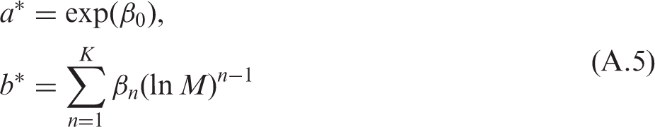
(A4) The validity of a simple allometric relationship (A.1) is supported by numerous experimental observations. However, the experimental data also suggest deviations from this simple linear behaviour (e.g. Kolokotrones et al., 2010). Based on experimentally observed non-linearity of the allometric data, straightforward polynomial generalisations of linear regression may be used (Ulanovsky, 2016) to test statistical significance of non-linear effects in allometric relationships:
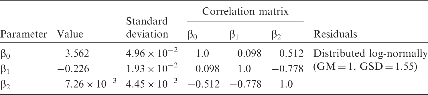
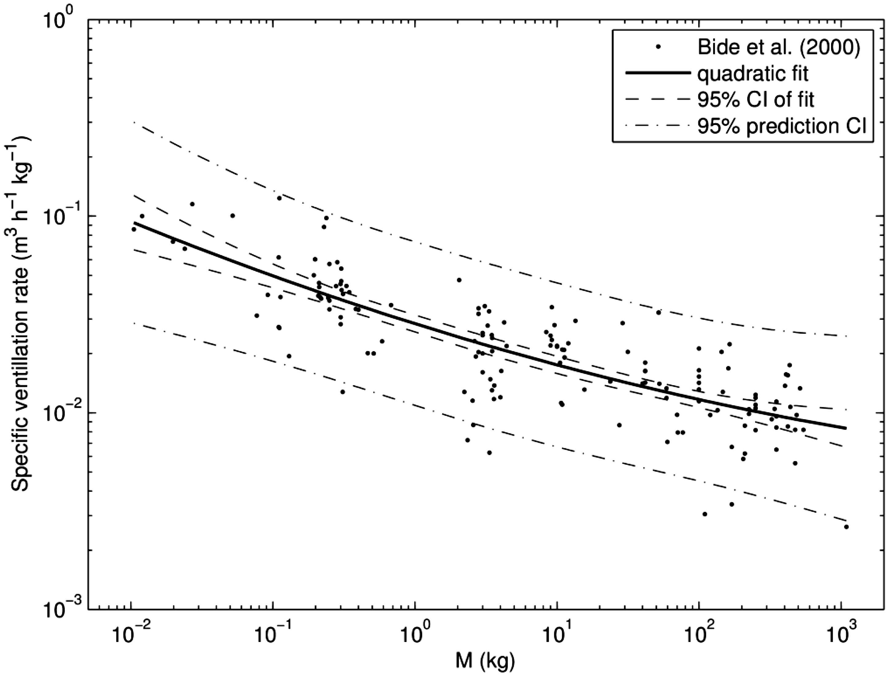
(A5) Generalised allometric Eqs. (A.4) and (A.5) were used to approximate breathing rates for terrestrial mammals using data from Bide et al. (2000), who assembled a dataset from 146 studies covering 2616 animals and 18 species ranging from mice at 12 g body mass to horses and a giraffe at ca. 500 kg body mass. The breathing rate data from Bide et al. (2000) were normalised per body mass and refitted (without excluding so-called ‘outliers’) using polynomial regression of logarithmically transformed variables. Polynomials with degrees from 0 to 3 have been applied, and the second-order polynomial has been found as the best model, based on the Akaike information criterion (AIC) (e.g. Anderson, 2008). Residuals have been found to be distributed normally (see parameters in Table A.1). Consequently, breathing rates for terrestrial mammals can be represented as follows:
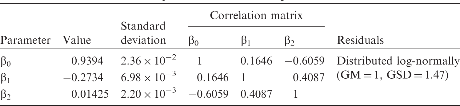
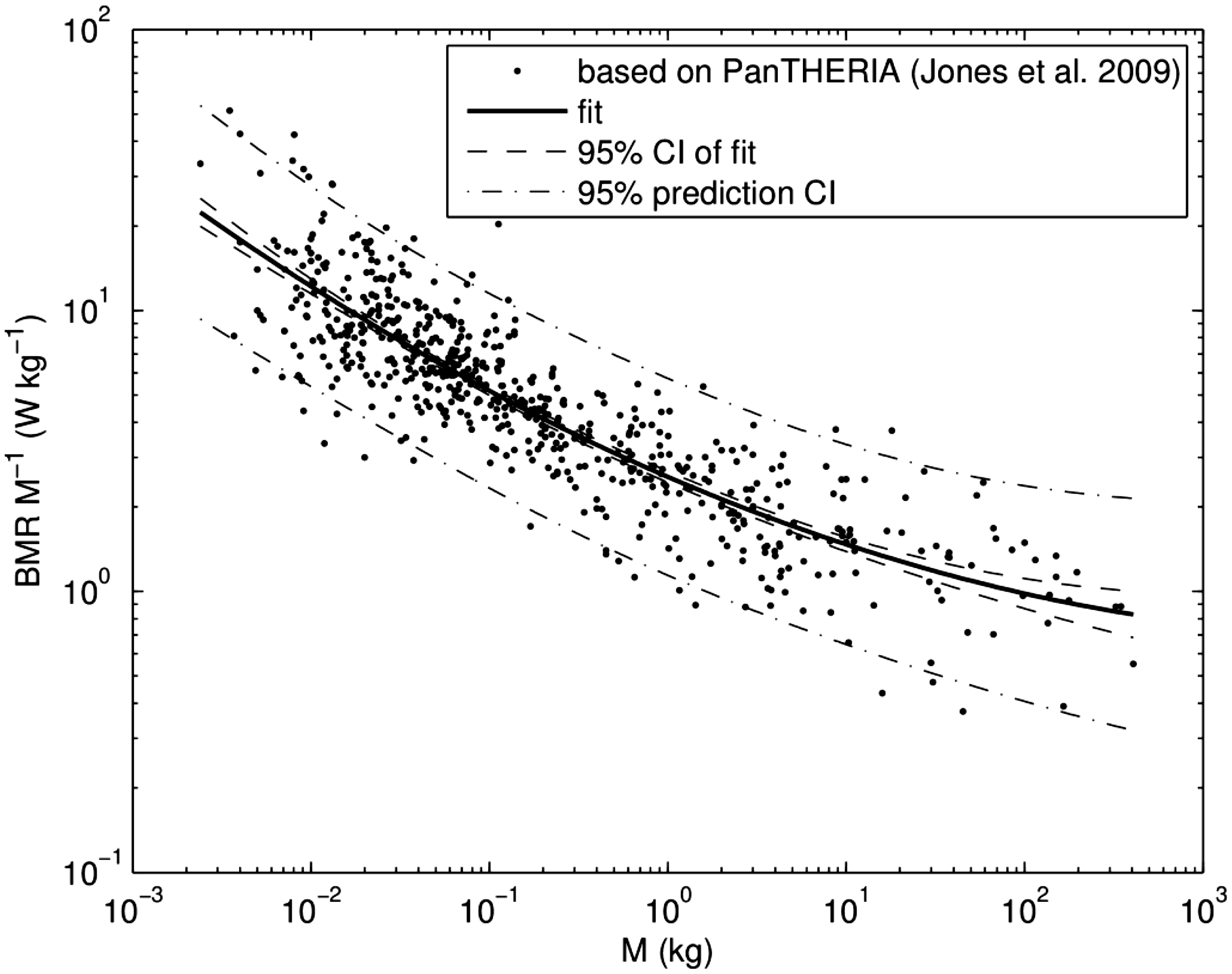
(A6) The dashed lines in Fig. A.1 indicate the 95% confidence intervals for the predicted dependence, which should not be confused with 95% prediction intervals, shown as dash-dotted lines, as the latter represents a variance of the sample on which the regression is constructed. In the case of a zero-order polynomial, these correspond to conventional variance of the sample mean and the sample variance. Variability can be characterised by a geometric standard deviation (GSD) of 1.55, which means that the ratio of the 97.5% to 2.5% percentiles equals approximately 5.6. (A7) Another example of how the generalised allometric relationships describe non-linear effects observed in biological data can be shown using an approximation of the basal metabolic rate (BMR) for terrestrial mammals. As suggested by Kleiber (1975), the specific BMR (i.e. energy of metabolism per unit body mass) can serve as an indicator of rates of biological processes resulting in elimination of substances from the organism (Kleiber, 1975; Fagerström et al., 1977). Thus, the BMR can be used for scaling biological half-time of well-studied mammals (e.g. mouse, dog, human) to other animals for which no sufficient information exists. (A8) Fitting has been performed using the measured BMR included in the PanTHERIA database (Jones et al., 2009), which includes data for mammals with body masses from grams to hundreds of kilograms. For these animals, the BMR is strongly correlated with mass, and varies by four orders of magnitude. The data have been fit using generalised allometric Eq. (A.4) and the resulting approximation appears as follows:
(A9) The data and the fitted approximation are shown in Fig. A.2. Fitted parameter values for ventilation rates for mammals. GM, geometric mean; GSD, geometric standard deviation. Parameter values of generalised allometric equation for basal metabolic rate. GM, geometric mean; GSD, geometric standard deviation. Fit of specific ventilation rates from Bide et al. (2000) using a generalised allometric equation [Eq. (A.6)]. CI, confidence interval. Scaled basal metabolic rate (BMR) for mammals. Points show data derived from the PanTHERIA database (Jones et al., 2009), the solid line is a fit using approximation [Eq. (A.7)], the dashed line shows the 95% confidence interval (CI) of the fit, and the dash-dotted line represents the 95% prediction bands.


A.1. References
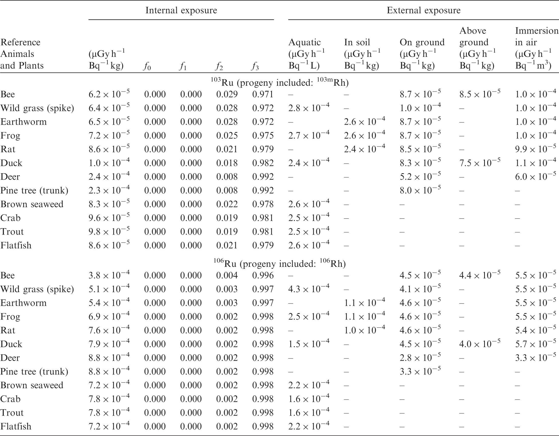
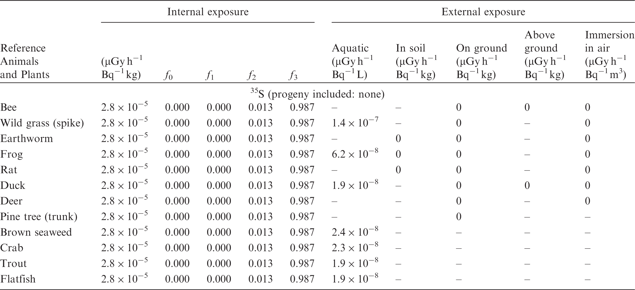
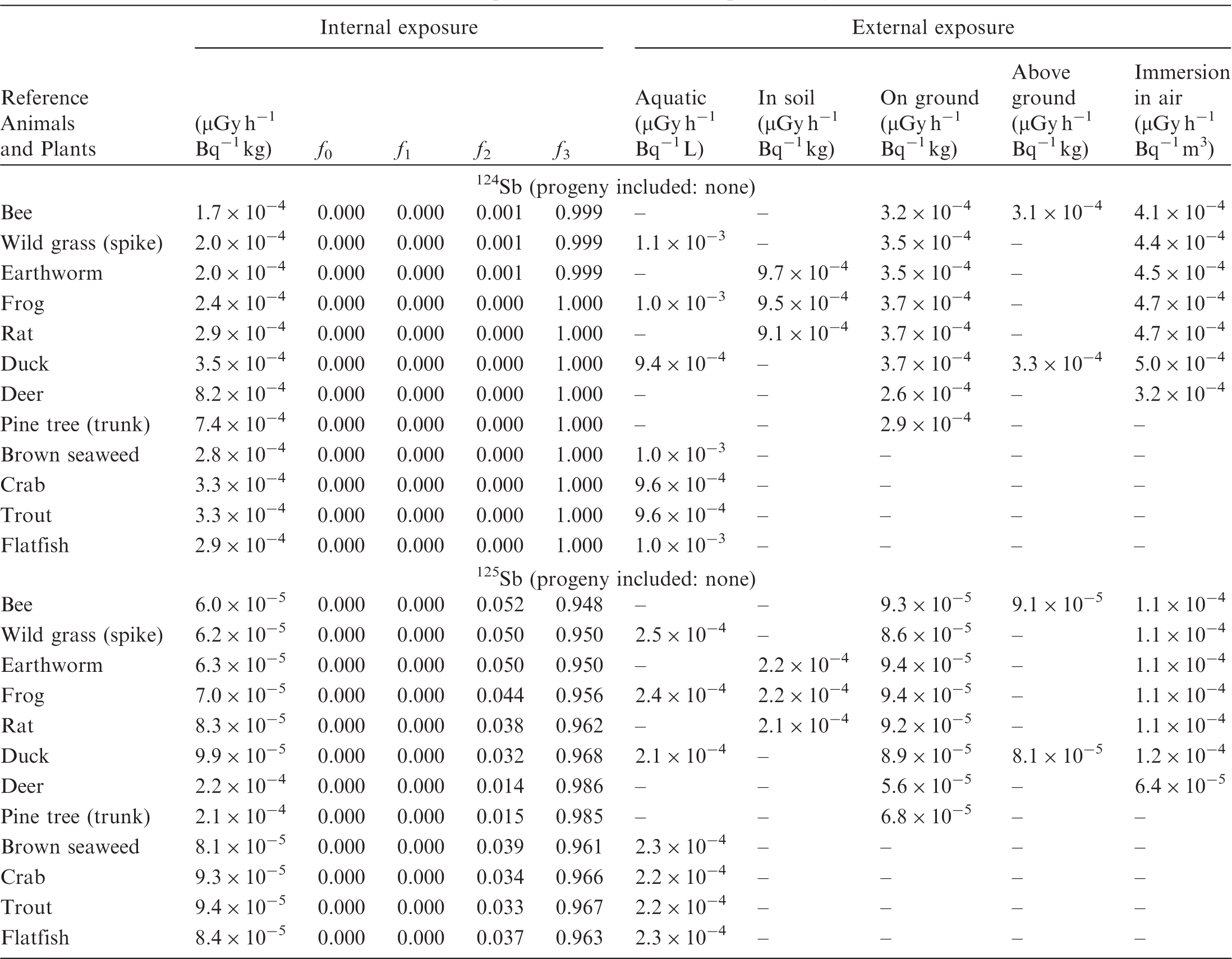
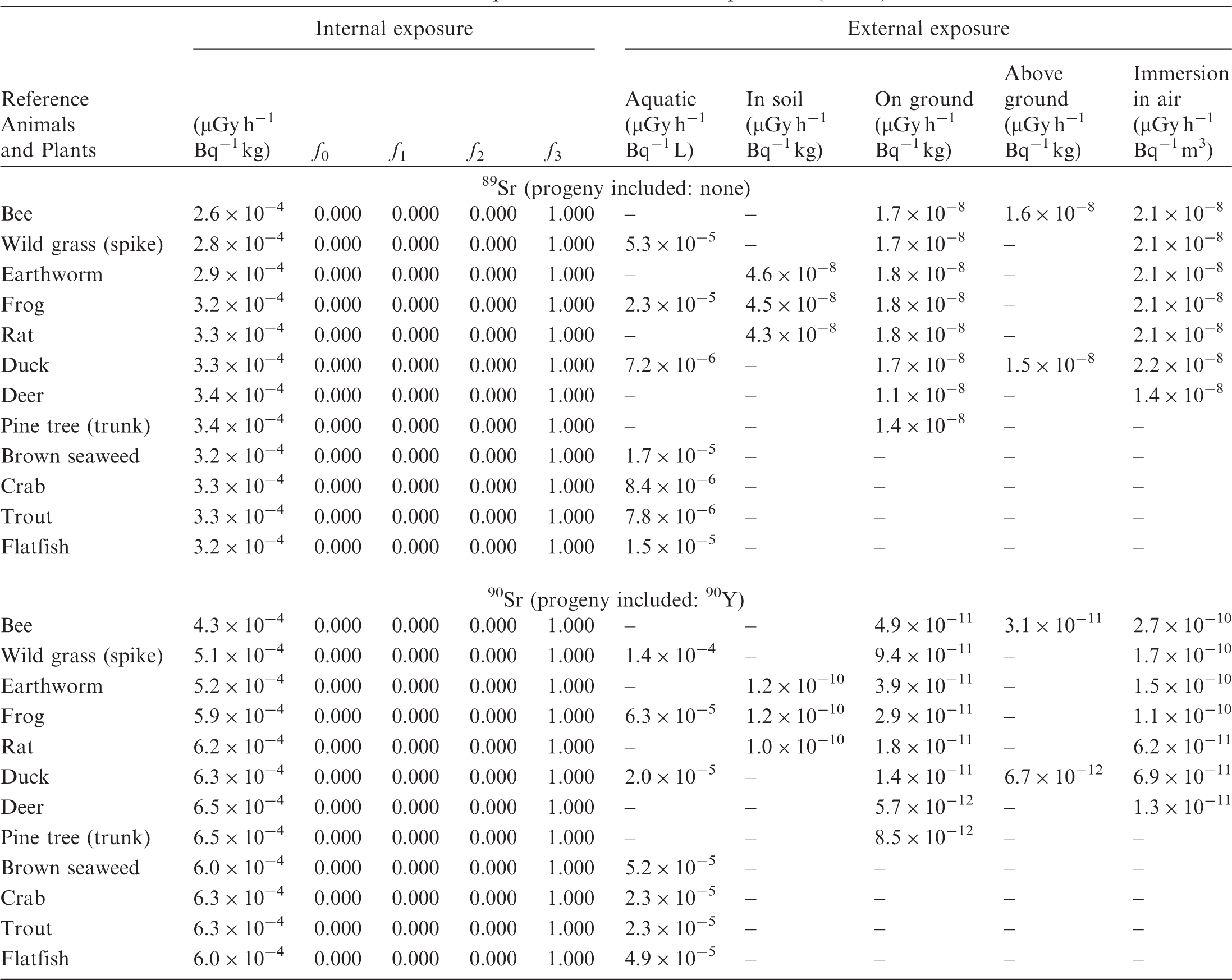
ANNEX B. DOSE COEFFICIENTS FOR NON-HUMAN BIOTA
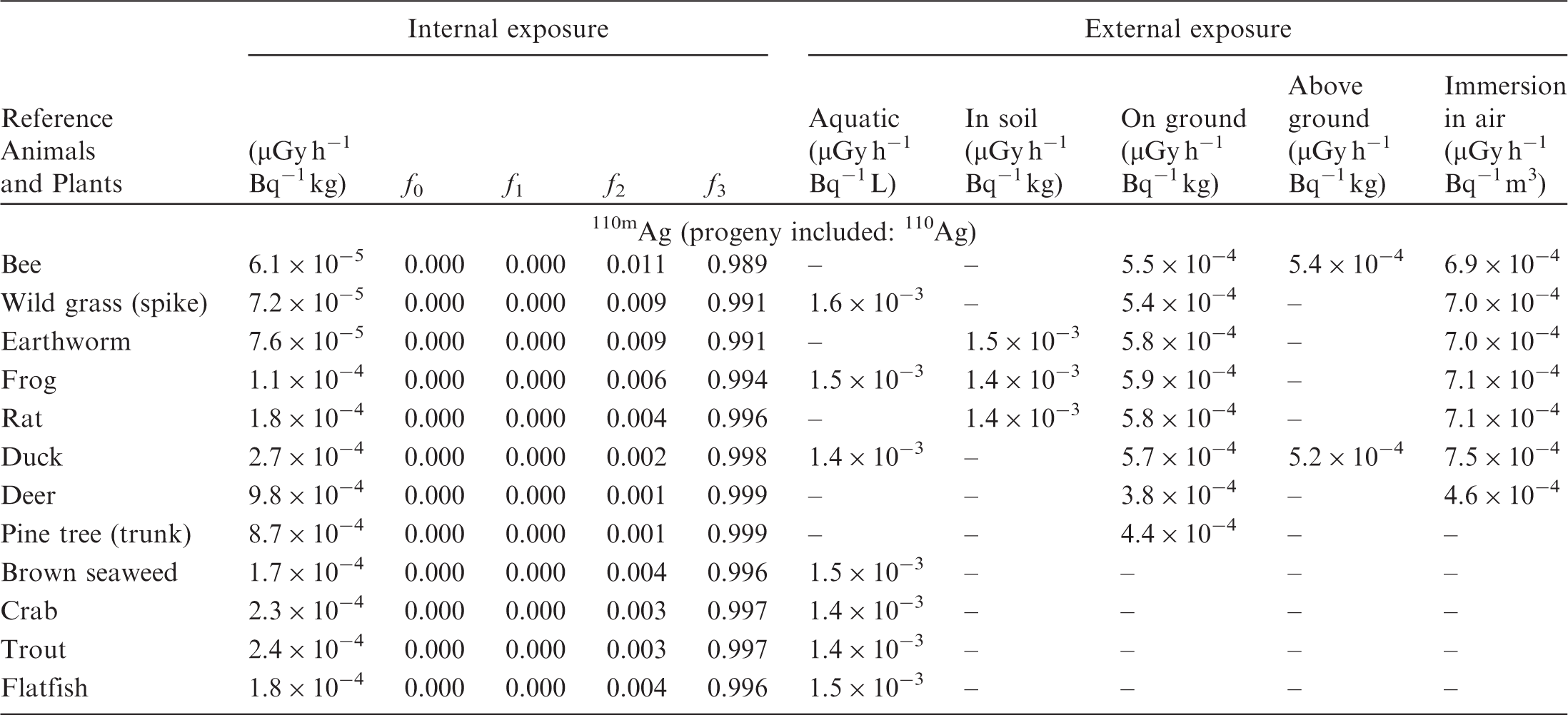
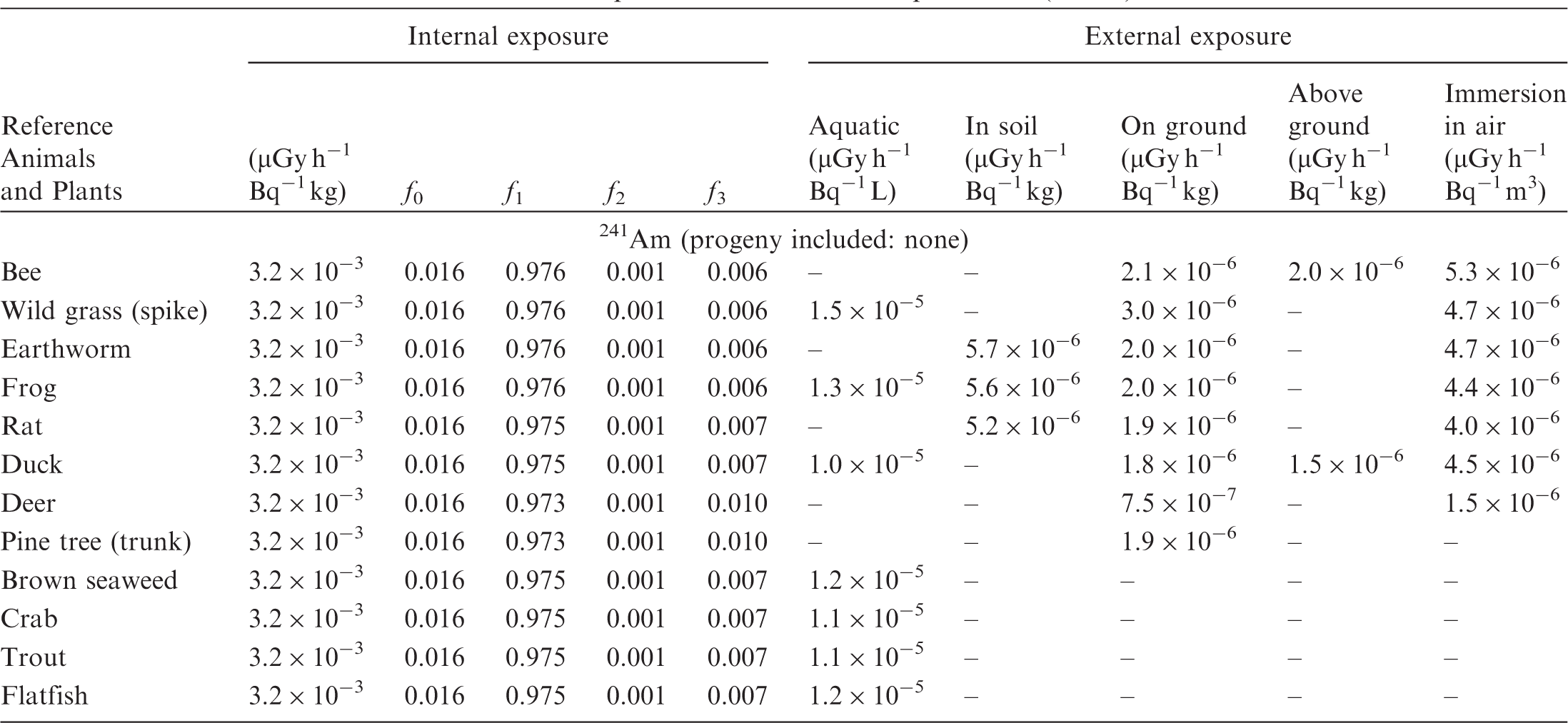
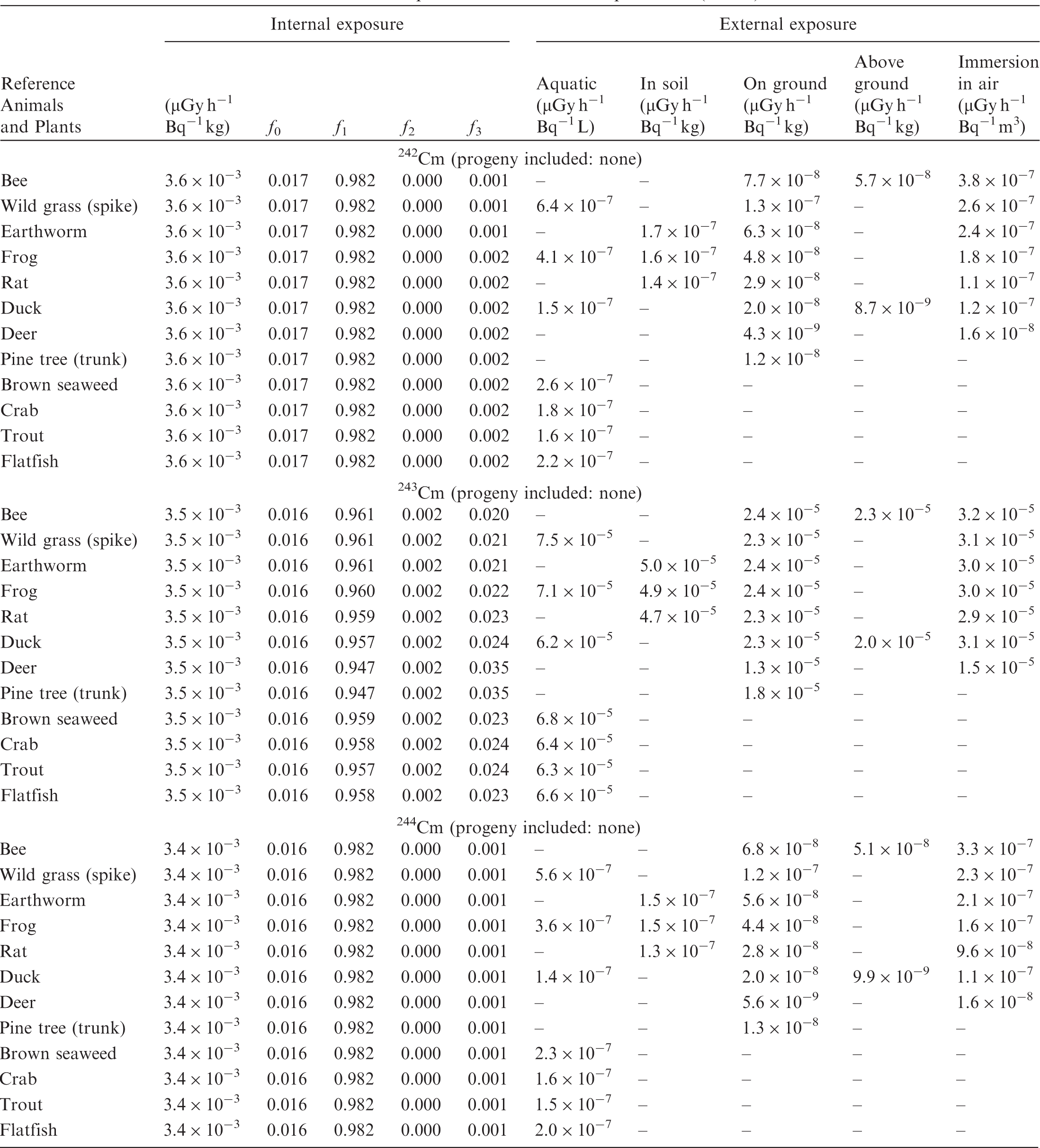
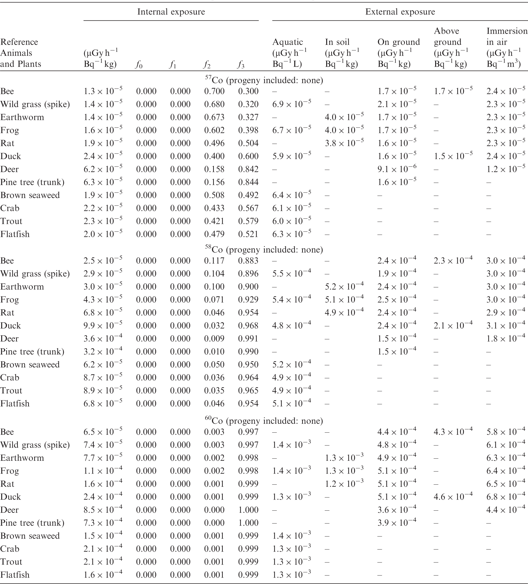
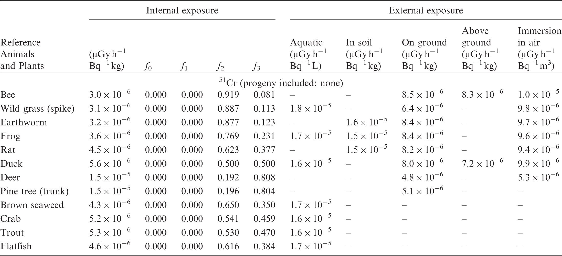
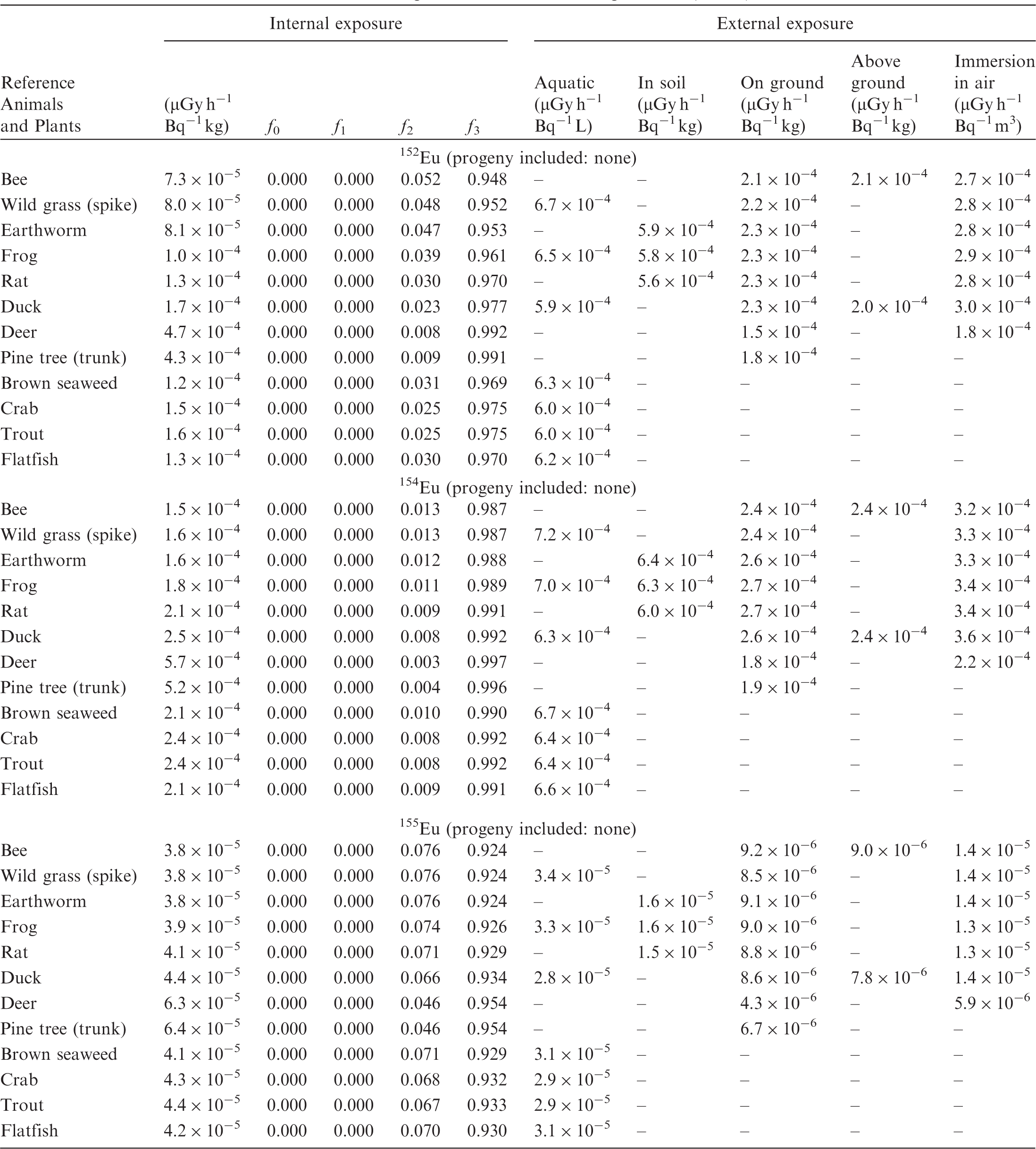
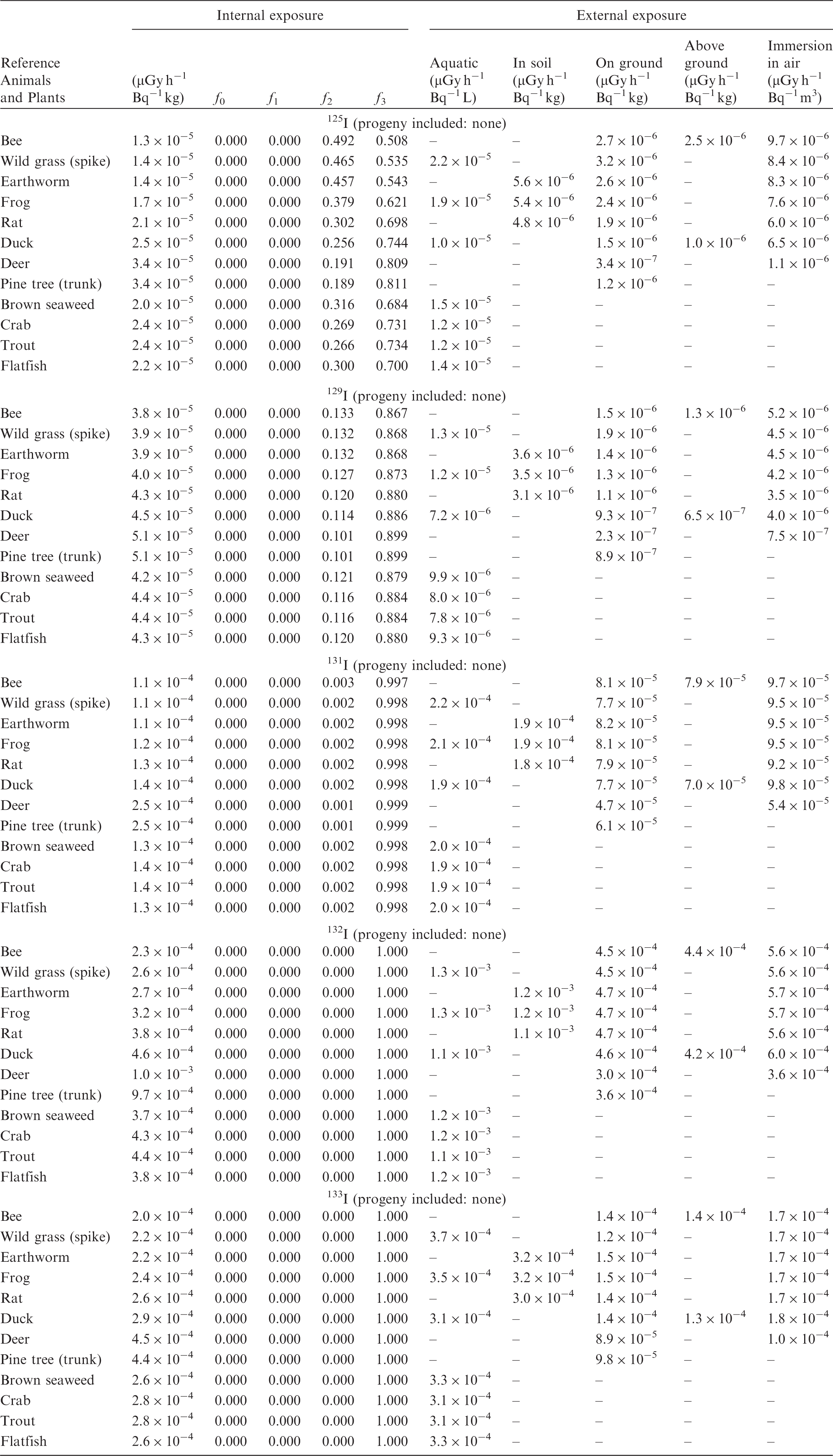
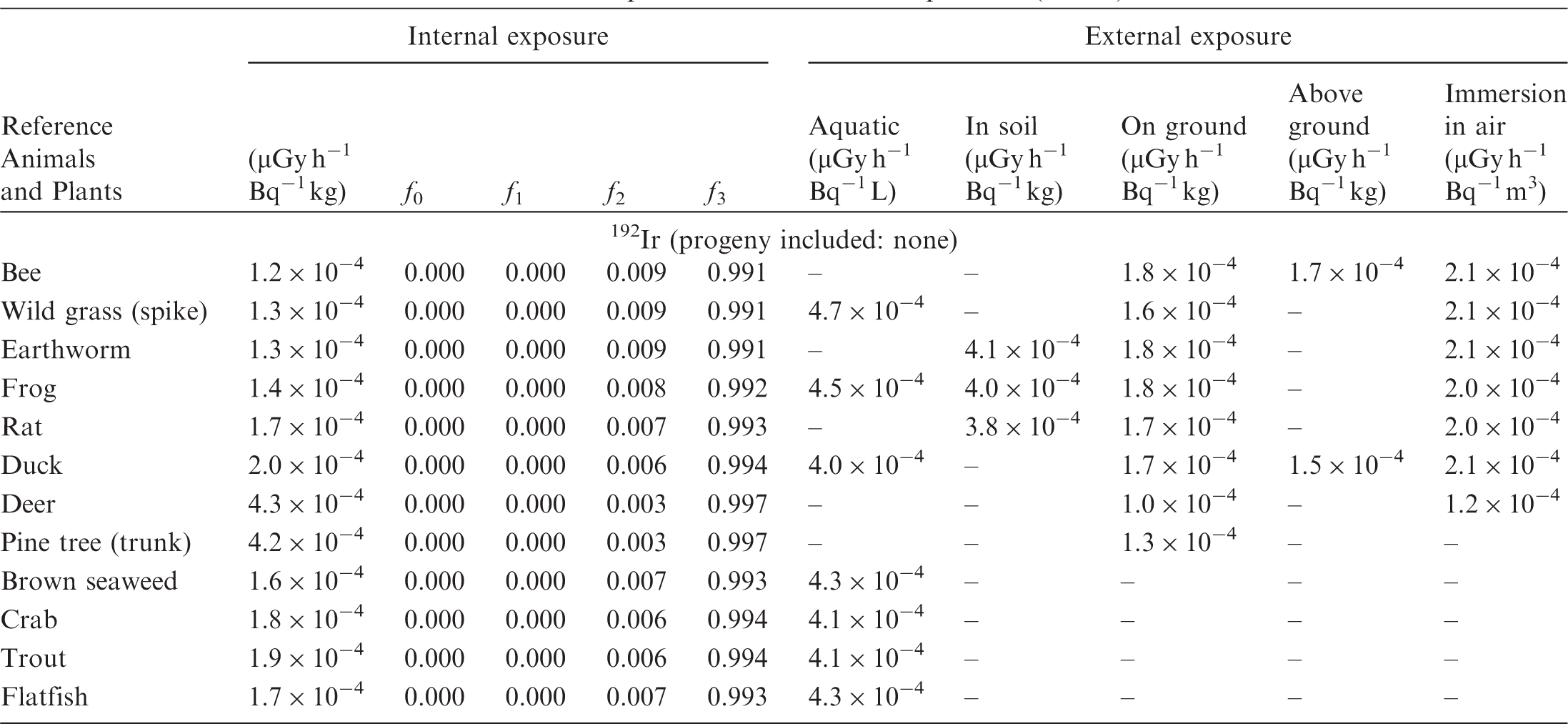
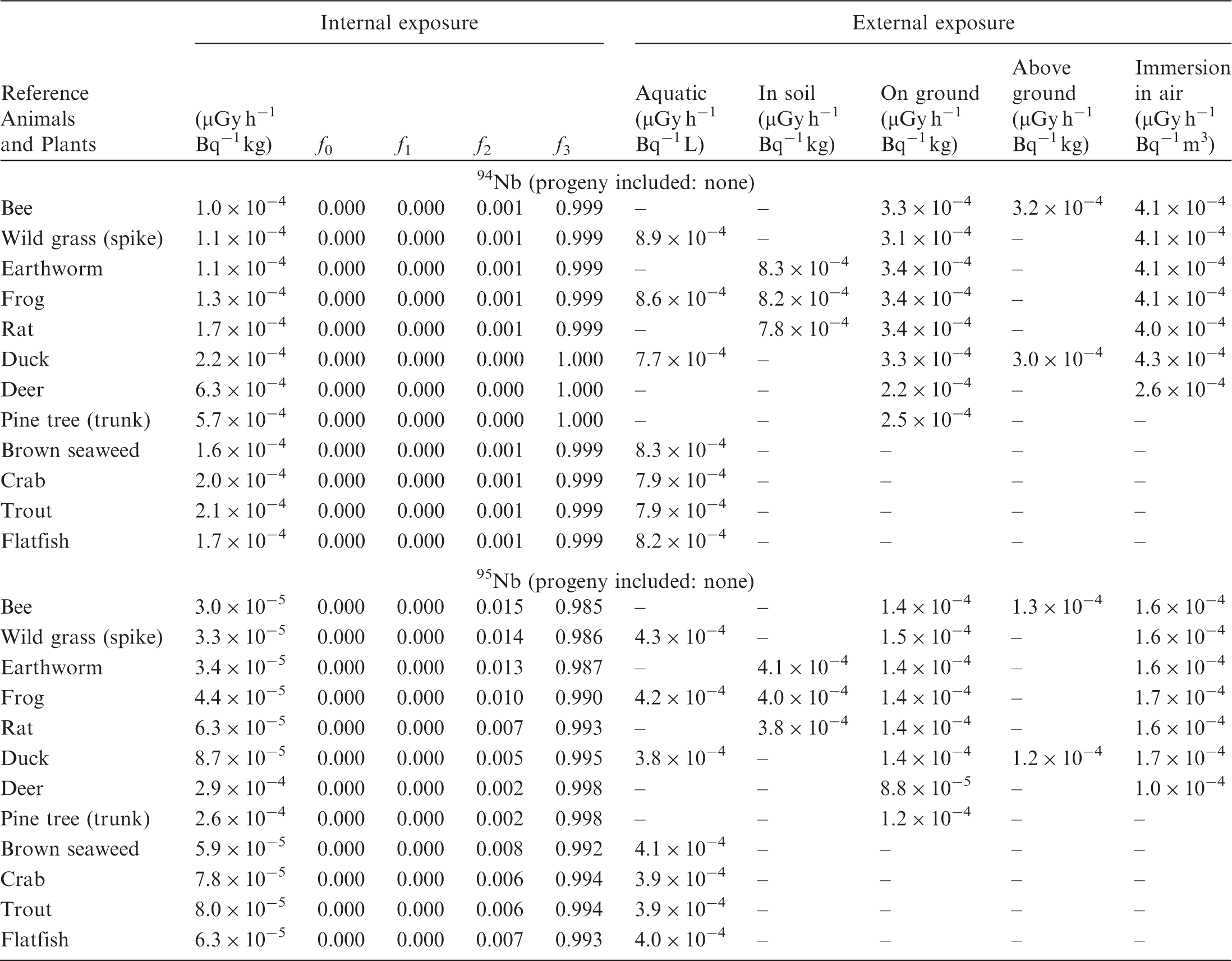
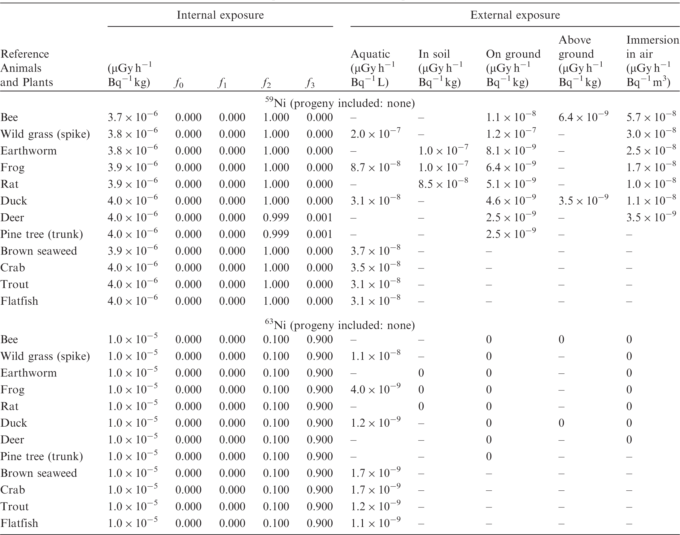
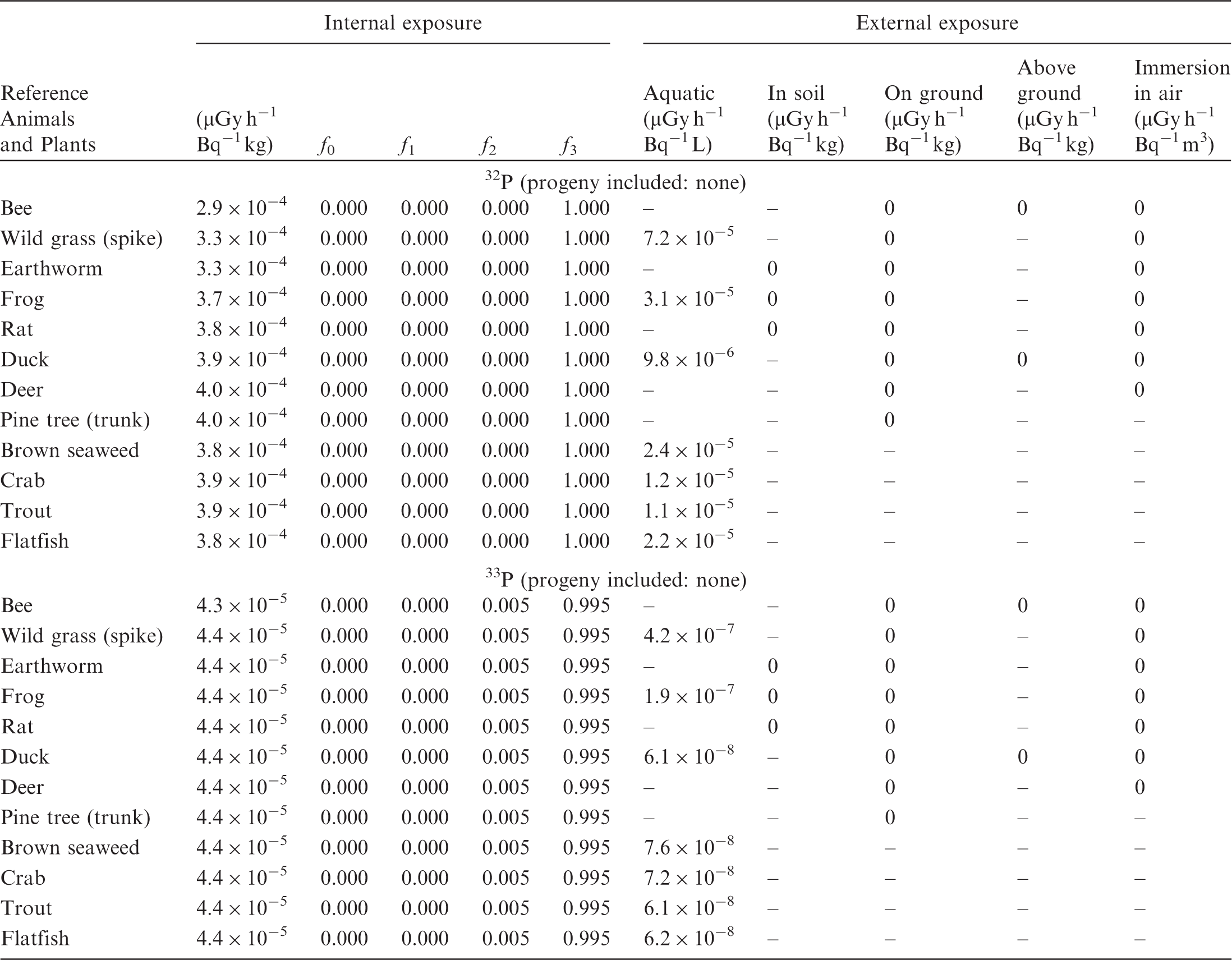
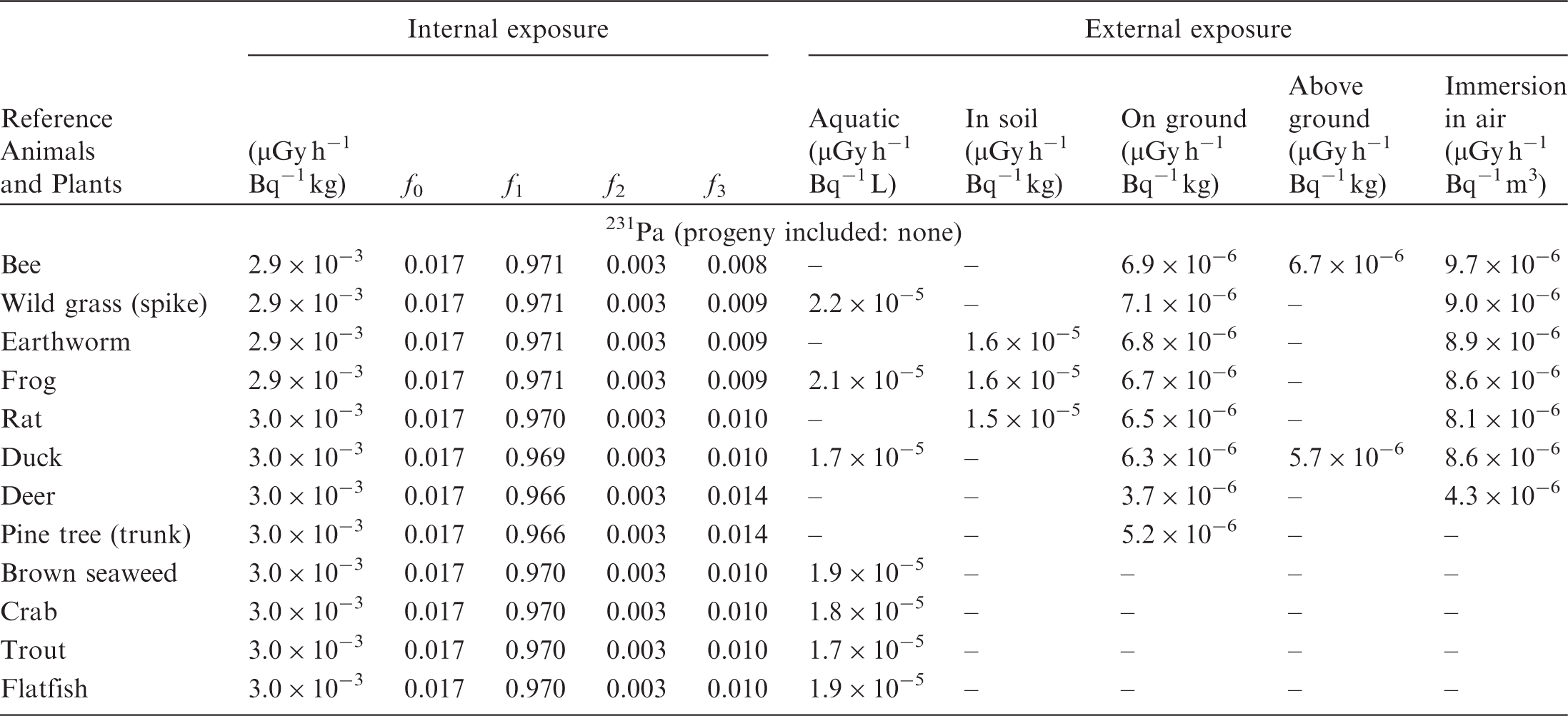
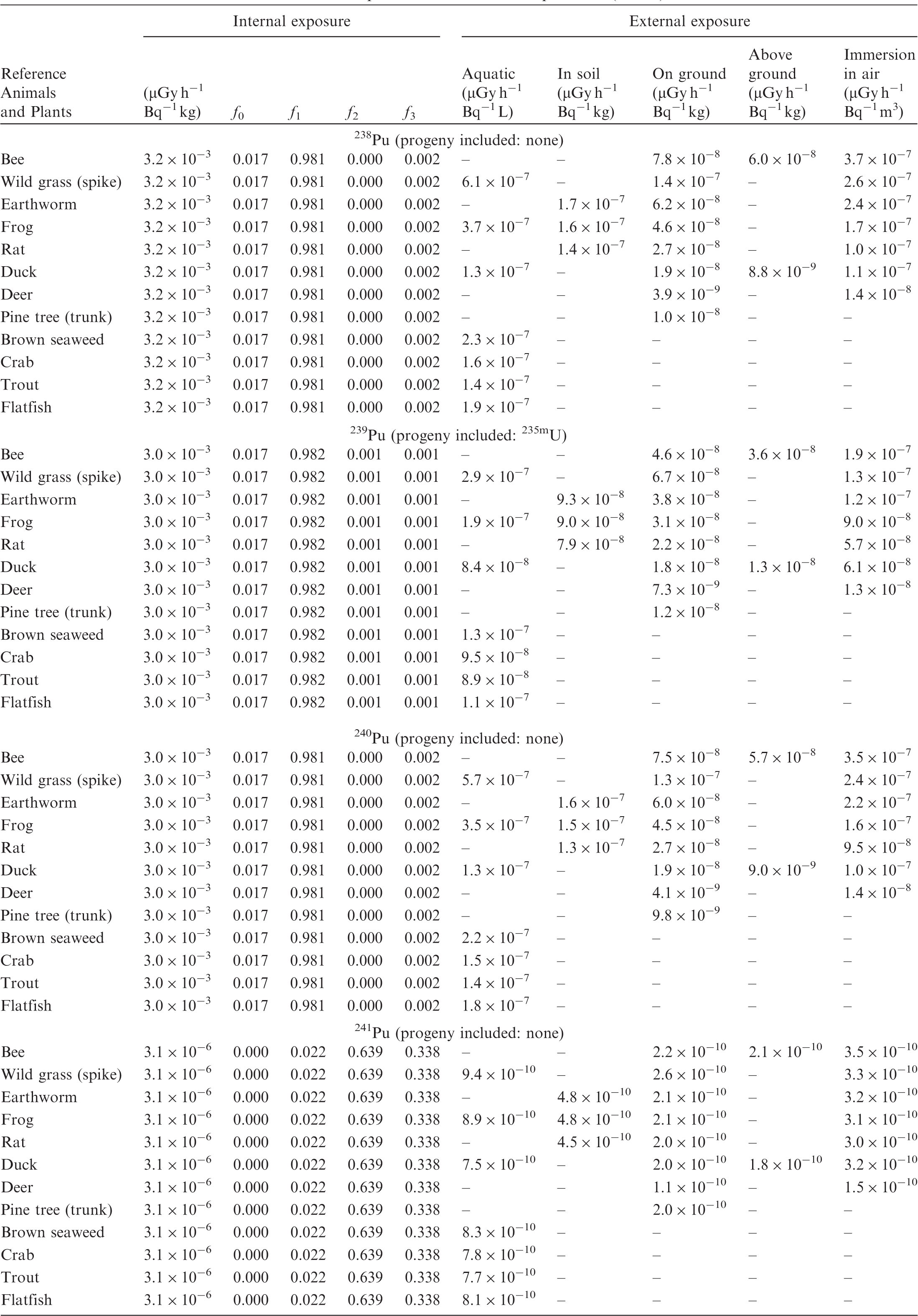
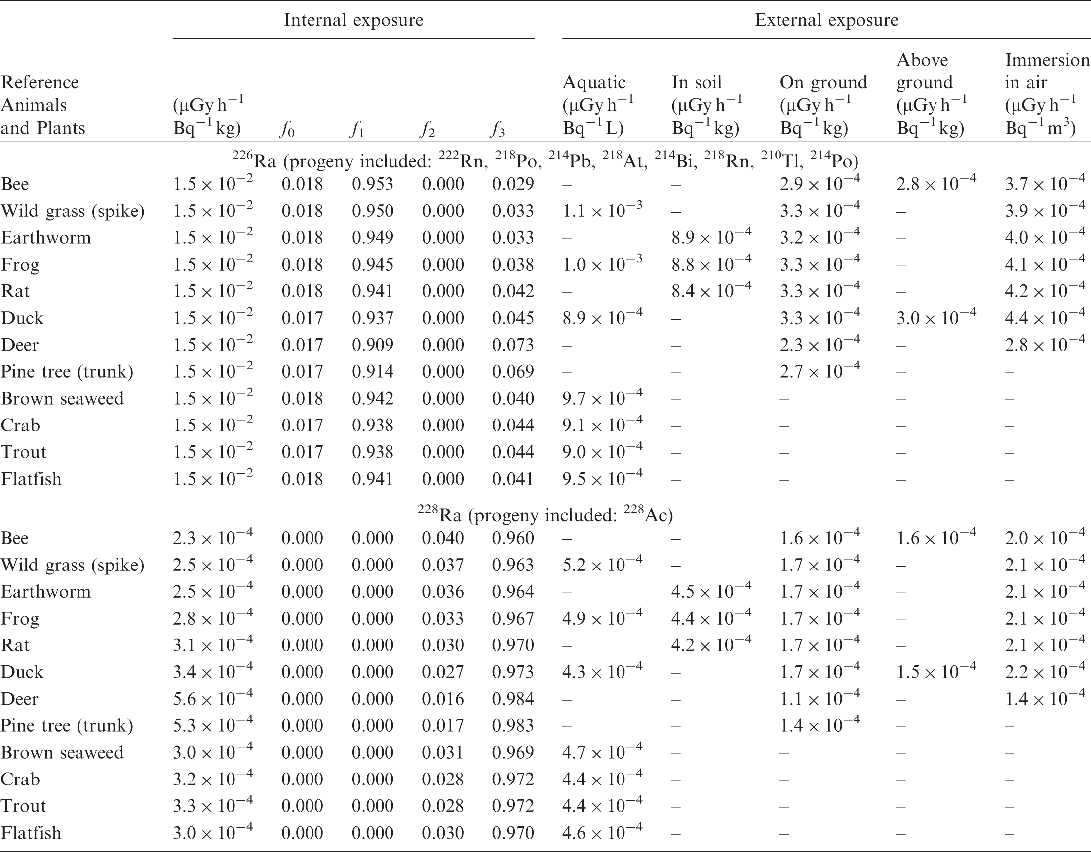
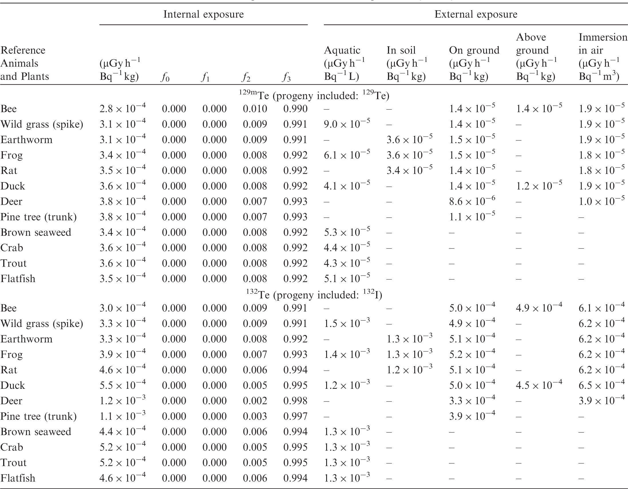
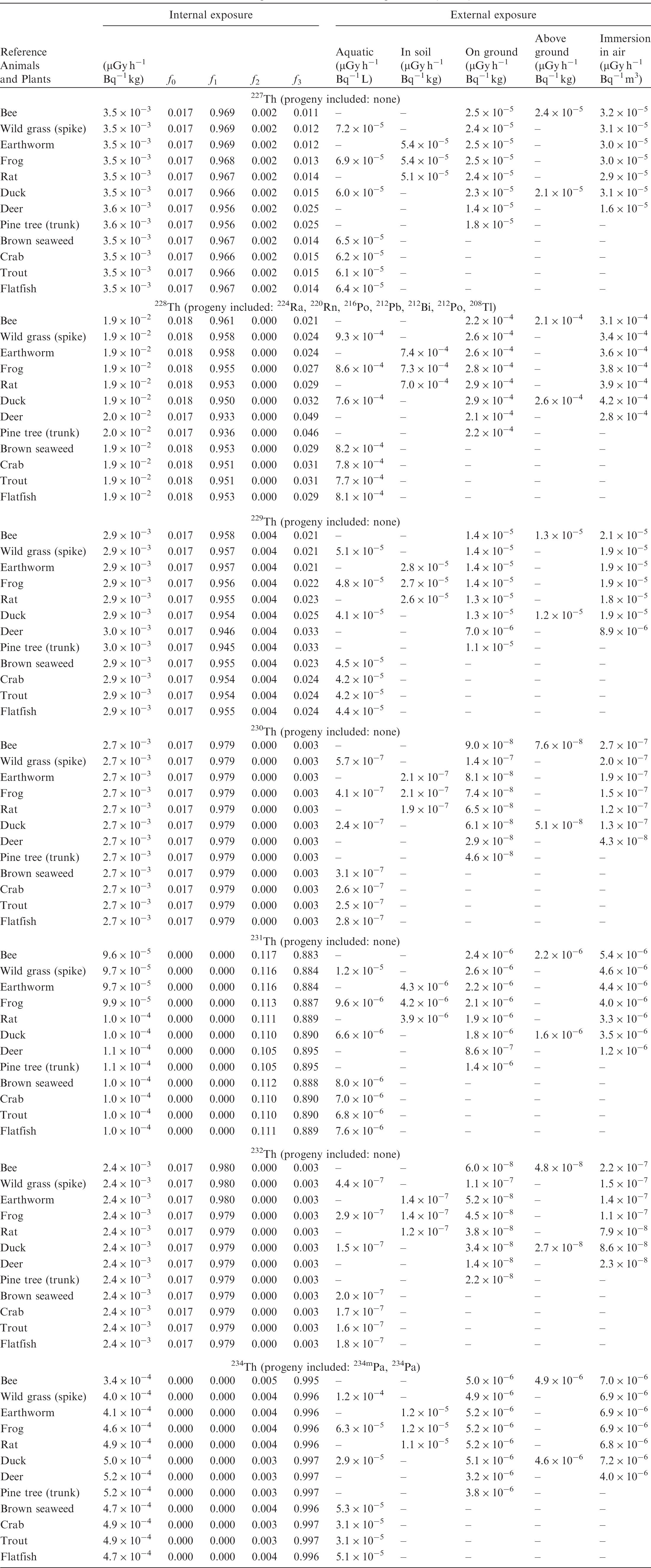
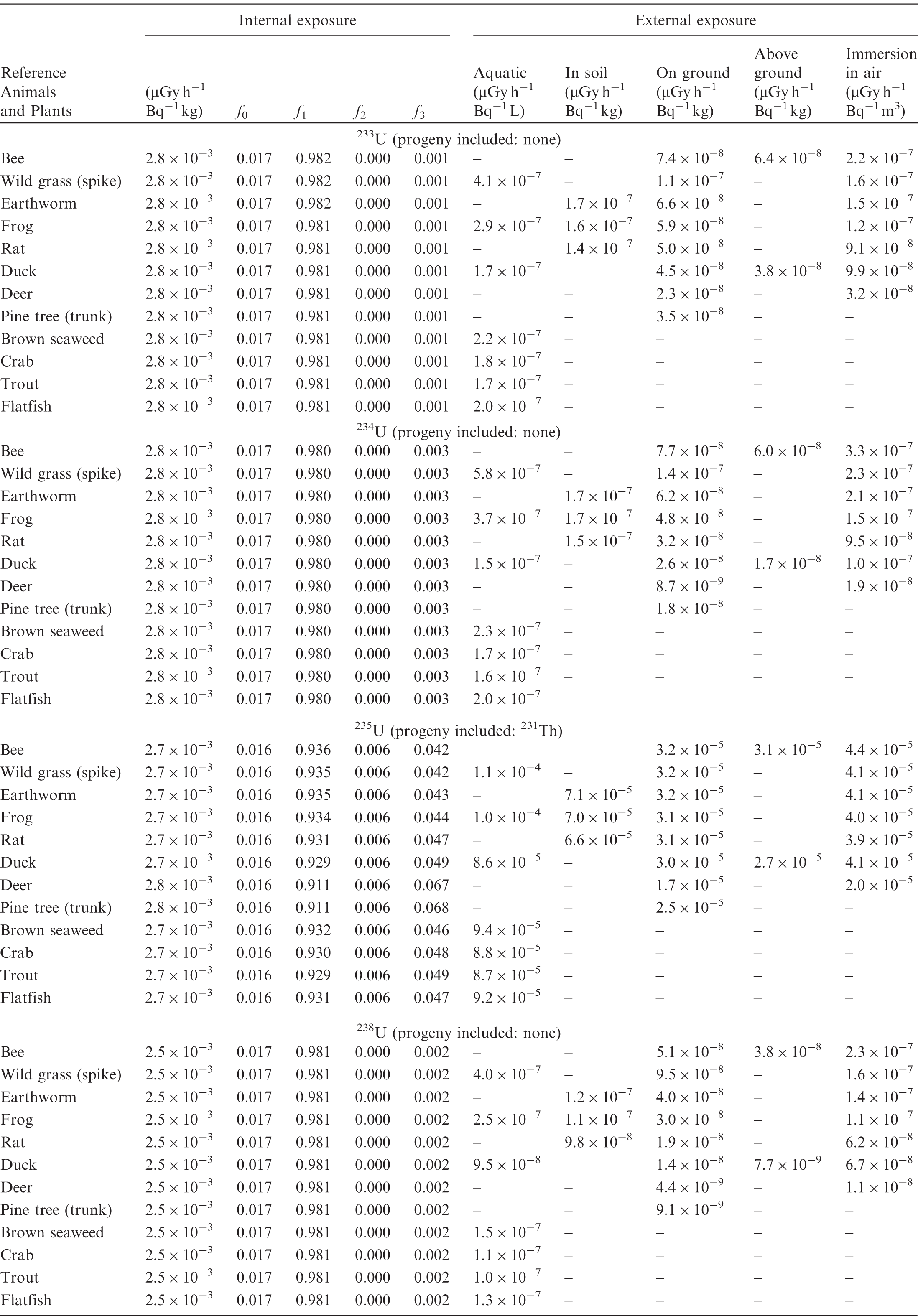
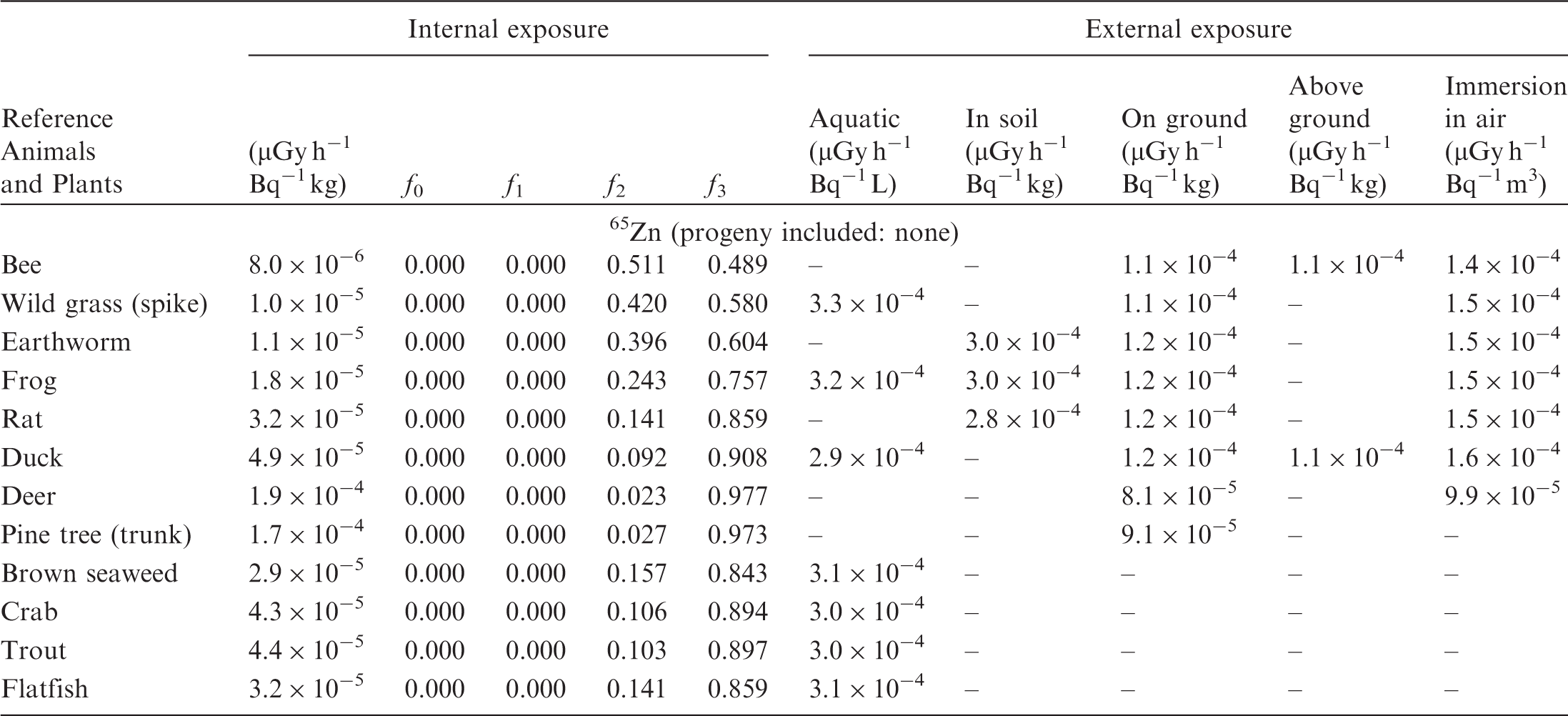
(B1) DCs shown in the following tables are presented as dose rates (µGy h−1) per unit activity concentration in the given media, i.e. Bq kg−1 for internal exposure and external exposure of terrestrial organisms, Bq L−1 for external exposure of aquatic organisms, and Bq m−3 for external exposure of terrestrial organisms immersed in radioactively contaminated air above the ground surface. (B2) DCs for external exposure of aquatic organisms are computed for infinite water medium. DCs can also be applied to assess external exposure from radioactivity in bed sediments, provided that density and chemical composition of the sediments are close to those of water medium. (B3) DCs for external exposure of terrestrial organisms are presented for exposure: ‘in soil’: for organisms exposed in the middle of a 50-cm-thick uniform source in soil; ‘on ground’: for organisms exposed on the ground surface to a 10-cm-thick uniform source in soil; ‘above ground’: for organisms exposed at a specified height (bee at 2 m, duck at 10 m) above the ground surface to a 10-cm-thick uniform source in soil; and ‘immersion in air’: for organisms exposed on or above the ground surface to uniformly contaminated ambient air. (B4) The energy emitted by radioactive progeny is added to DCs according to the method used in Publication 108 (ICRP, 2008b), i.e. the decay chain is truncated at the first daughter nuclide with physical half-life of >10 days, or longer than that of the parent nuclide, and equilibrium conditions are assumed to exist between the parent and daughters in the truncated decay chain. (B5) The organisms listed in the tables are those from the terrestrial environment, followed by aquatic organisms. Each group is sorted according to increasing organism mass. DCs for internal exposure are followed by a set of fractions representing the contributions of various radiation types to the internal dose. Specifically, f0 represents the contribution of fission fragments and alpha-recoil nuclei, f1 represents alpha particles, f2 represents low-energy beta and gamma radiation (E <10 keV), and f3 represents other beta and gamma radiation (E >10 keV). The fractions can be used to modify the absorbed dose rate by radiation weighting factors, which account for the different radiobiological effectiveness of various radiation types. Dose coefficients for non-human biota exposed to radioactive isotopes of Ag (Z = 47). Dose coefficients for non-human biota exposed to radioactive isotopes of Am (Z = 95). Dose coefficients for non-human biota exposed to radioactive isotopes of Ba (Z = 56). Dose coefficients for non-human biota exposed to radioactive isotopes of C (Z = 6). Dose coefficients for non-human biota exposed to radioactive isotopes of Ca (Z = 20). Dose coefficients for non-human biota exposed to radioactive isotopes of Cd (Z = 48). Dose coefficients for non-human biota exposed to radioactive isotopes of Ce (Z = 58). Dose coefficients for non-human biota exposed to radioactive isotopes of Cf (Z = 98). Dose coefficients for non-human biota exposed to radioactive isotopes of Cl (Z = 17). Dose coefficients for non-human biota exposed to radioactive isotopes of Cm (Z = 96). Dose coefficients for non-human biota exposed to radioactive isotopes of Co (Z = 27). Dose coefficients for non-human biota exposed to radioactive isotopes of Cr (Z = 24). Dose coefficients for non-human biota exposed to radioactive isotopes of Cs (Z = 55). Dose coefficients for non-human biota exposed to radioactive isotopes of Eu (Z = 63). Dose coefficients for non-human biota exposed to radioactive isotopes of H (Z = 1). Dose coefficients for non-human biota exposed to radioactive isotopes of I (Z = 53). Dose coefficients for non-human biota exposed to radioactive isotopes of Ir (Z = 77). Dose coefficients for non-human biota exposed to radioactive isotopes of K (Z = 19). Dose coefficients for non-human biota exposed to radioactive isotopes of La (Z = 57). Dose coefficients for non-human biota exposed to radioactive isotopes of Mn (Z = 25). Dose coefficients for non-human biota exposed to radioactive isotopes of Nb (Z = 41). Dose coefficients for non-human biota exposed to radioactive isotopes of Ni (Z = 28). Dose coefficients for non-human biota exposed to radioactive isotopes of Np (Z = 93). Dose coefficients for non-human biota exposed to radioactive isotopes of P (Z = 15). Dose coefficients for non-human biota exposed to radioactive isotopes of Pa (Z = 91). Dose coefficients for non-human biota exposed to radioactive isotopes of Pb (Z = 82). Dose coefficients for non-human biota exposed to radioactive isotopes of Po (Z = 84). Dose coefficients for non-human biota exposed to radioactive isotopes of Pu (Z = 94). Dose coefficients for non-human biota exposed to radioactive isotopes of Ra (Z = 88). Dose coefficients for non-human biota exposed to radioactive isotopes of Ru (Z = 44). Dose coefficients for non-human biota exposed to radioactive isotopes of S (Z = 16). Dose coefficients for non-human biota exposed to radioactive isotopes of Sb (Z = 51). Dose coefficients for non-human biota exposed to radioactive isotopes of Se (Z = 34). Dose coefficients for non-human biota exposed to radioactive isotopes of Sr (Z = 38). Dose coefficients for non-human biota exposed to radioactive isotopes of Tc (Z = 43). Dose coefficients for non-human biota exposed to radioactive isotopes of Te (Z = 52). Dose coefficients for non-human biota exposed to radioactive isotopes of Th (Z = 90). Dose coefficients for non-human biota exposed to radioactive isotopes of U (Z = 92). Dose coefficients for non-human biota exposed to radioactive isotopes of Zn (Z = 30). Dose coefficients for non-human biota exposed to radioactive isotopes of Zr (Z = 40).


ANNEX C. PROGRAMME BIOTADC – DOSE COEFFICIENTS FOR ENVIRONMENTAL EXPOSURE OF NON-HUMAN BIOTA
C.1. Introduction
(C1) The programme BiotaDC
1
© ICRP, 2016. Developed on behalf of ICRP by Alexander Ulanovsky and Alexander Ulanowski.
(C2) The programme originates from the dosimetric database developed in the FASSET and ERICA projects (Larsson, 2004, 2008) for terrestrial animals and plants. For aquatic organisms, the programme implements a technique based on an original set of computed doses for spherical shapes in an aquatic medium, and an analytical method to scale these to non-spherical and ellipsoidal shapes (Ulanovsky and Pröhl, 2006). The detailed overview of the methodology adopted by Publication 108 (ICRP, 2008b) can be found elsewhere (Ulanovsky et al., 2008; Ulanovsky and Pröhl, 2008). In the following years, more changes and improvements have been added to the tool, resulting in extension of the methodology used to assess external exposures of terrestrial animals to environmental sources of radiation (Ulanovsky, 2014).
(C3) The programme uses binary data files derived from Publication 107 (ICRP, 2008a) that contain data on radionuclide emissions, including discrete energy photon, electron, and alpha particles; continuous energy beta spectra; spontaneous fission energy yield; and energy of alpha-recoil nuclei.
(C4) The programme queries the database to construct a decay chain for the given parent nuclide, and to include radiations emitted both by the parent nuclide and its progeny into DC computation. The system of ordinary differential equations, describing the constructed decay chain, is solved (Strenge, 1997) to determine the activity of decay chain members either as transient values at a specified time after the beginning of the parent decay, or as integral values for a specified time interval. The decay chain can be truncated based on dosimetric criteria (i.e. removing daughters that contribute less than 10−9 to the total energy emitted by the full decay chain members). Alternatively, the decay chain can be truncated at the first daughter nuclide with physical half-life of >10 days, or longer than that of the parent nuclide. In the latter case, parent and residual daughters are assumed to be in secular equilibrium. This is the so-called ‘Publication 108 compatible’ approach that was originally implemented in the ERICA tool (Brown et al., 2008) and later used to calculate DCs in Publication 108 (ICRP, 2008b). This method is a simplified way to account for the contribution of radioactive progeny, and it should be noted that the method may result in implausible results for some exposure scenarios.
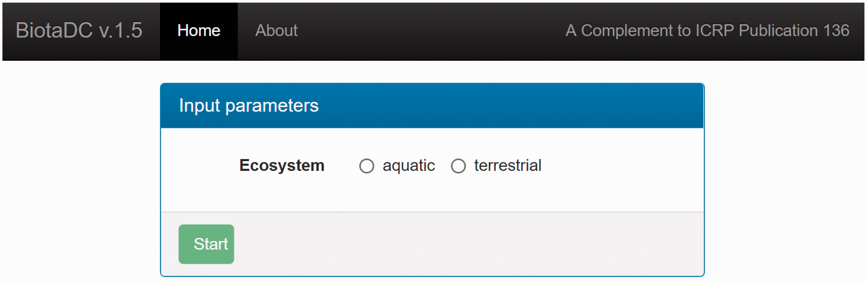
Initial screen of the programme after connecting to the website.
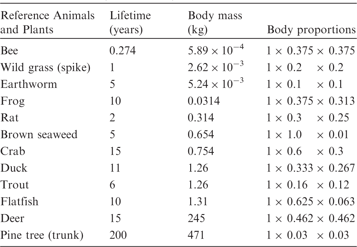
Lifetime, body mass, and shape parameters for Reference Animals and Plants (ICRP, 2008b).
C.2. Operation
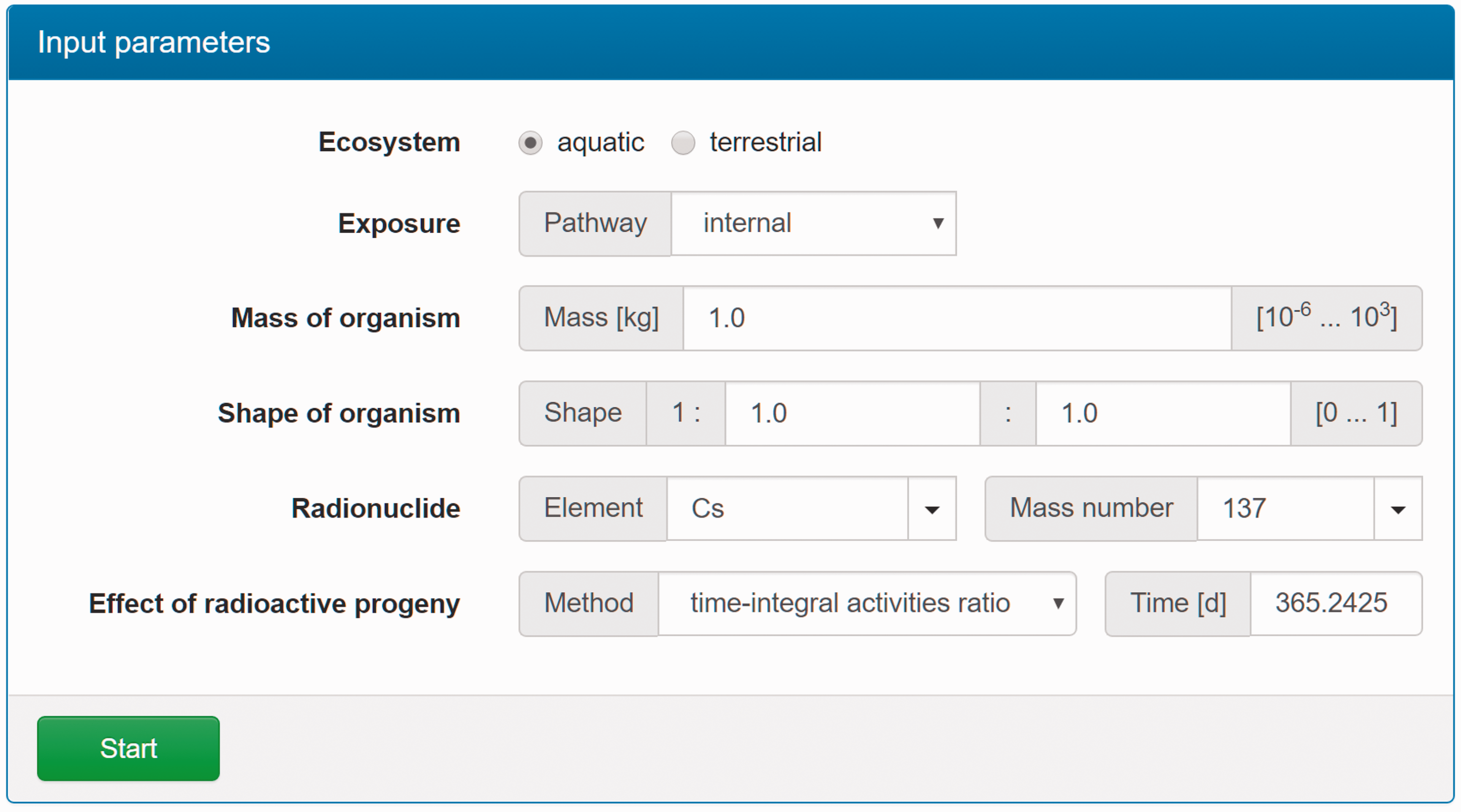
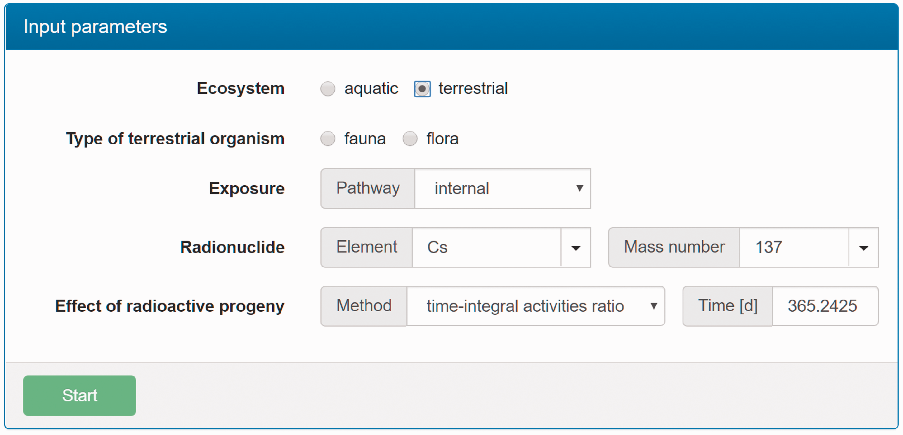
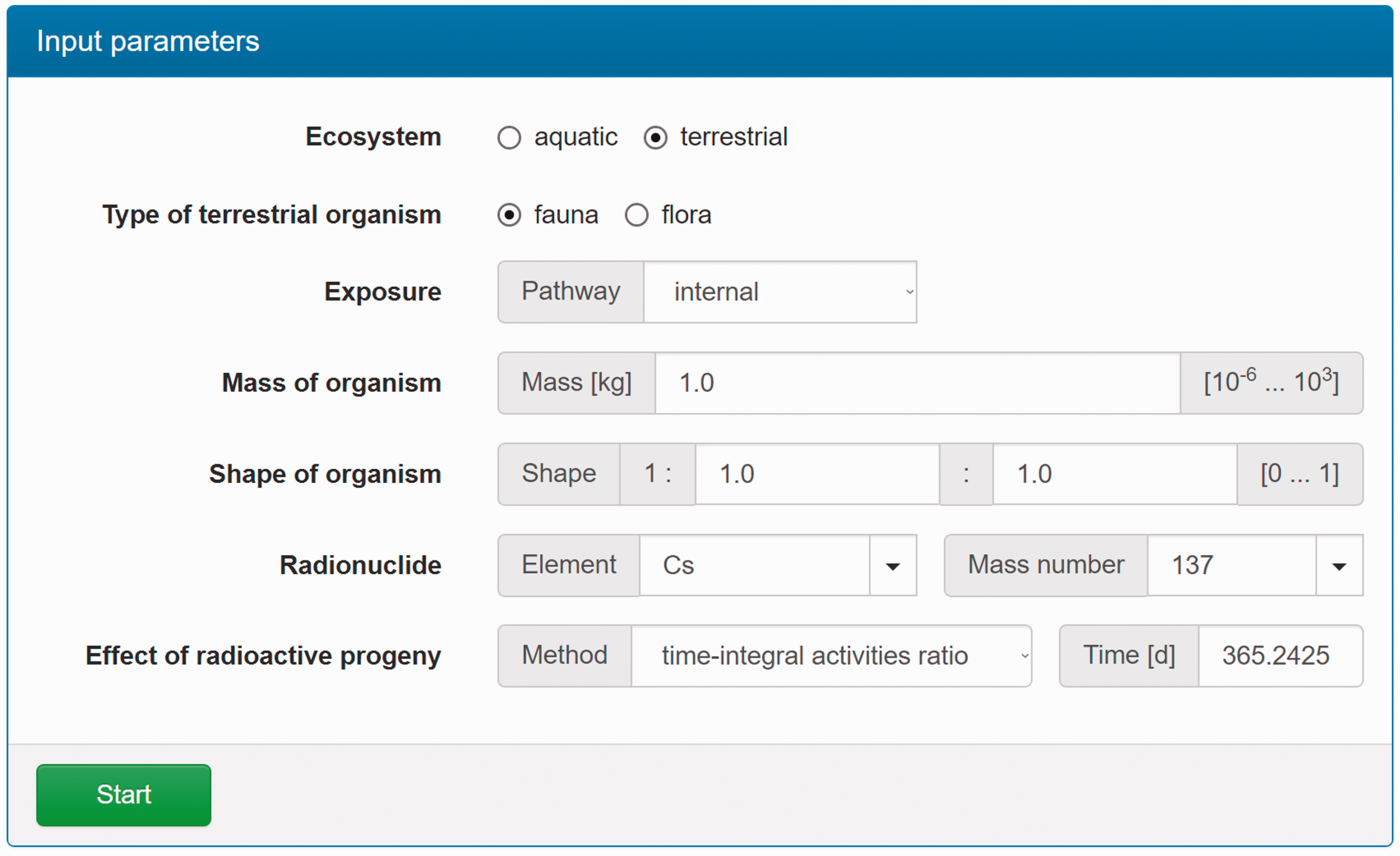
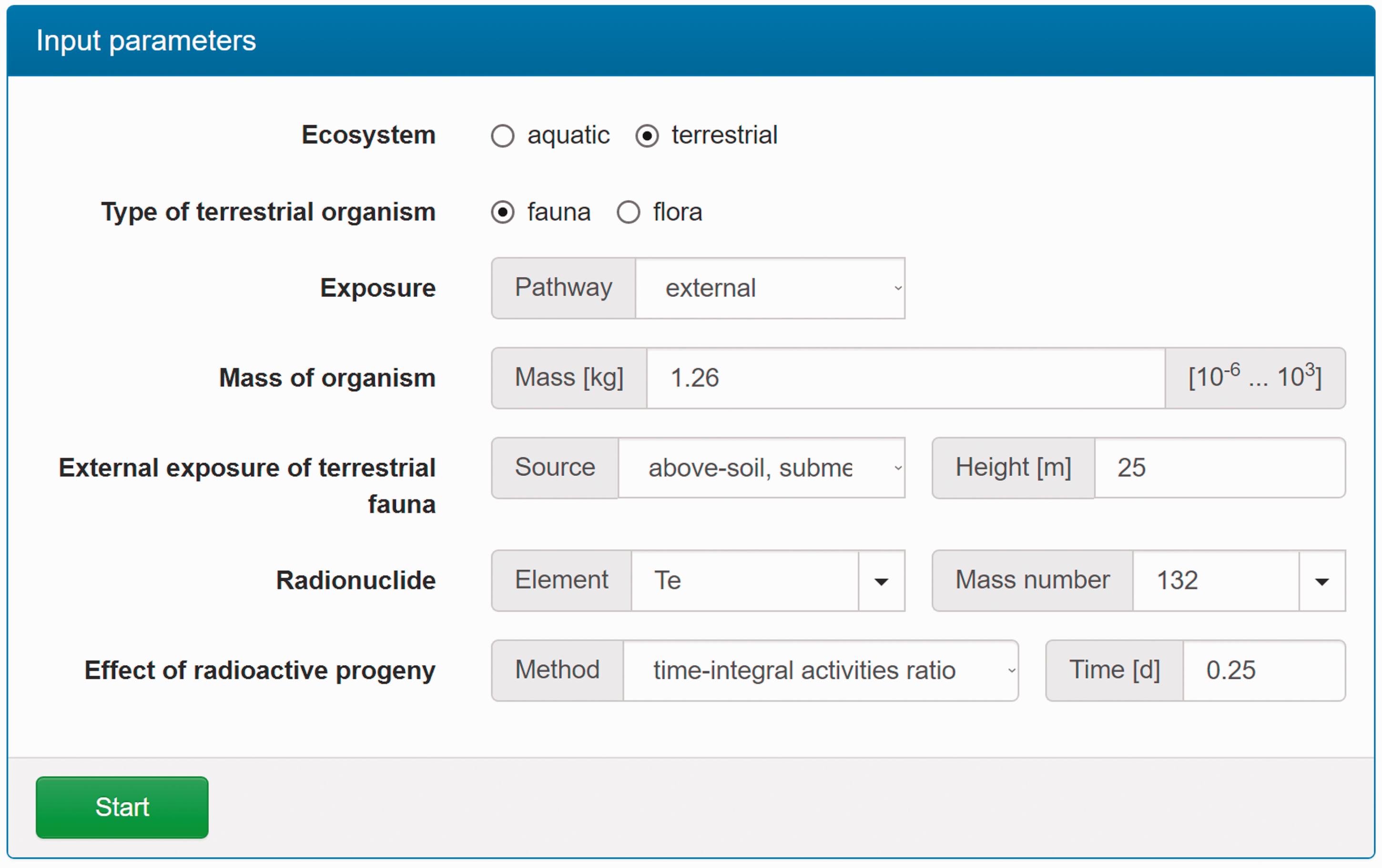
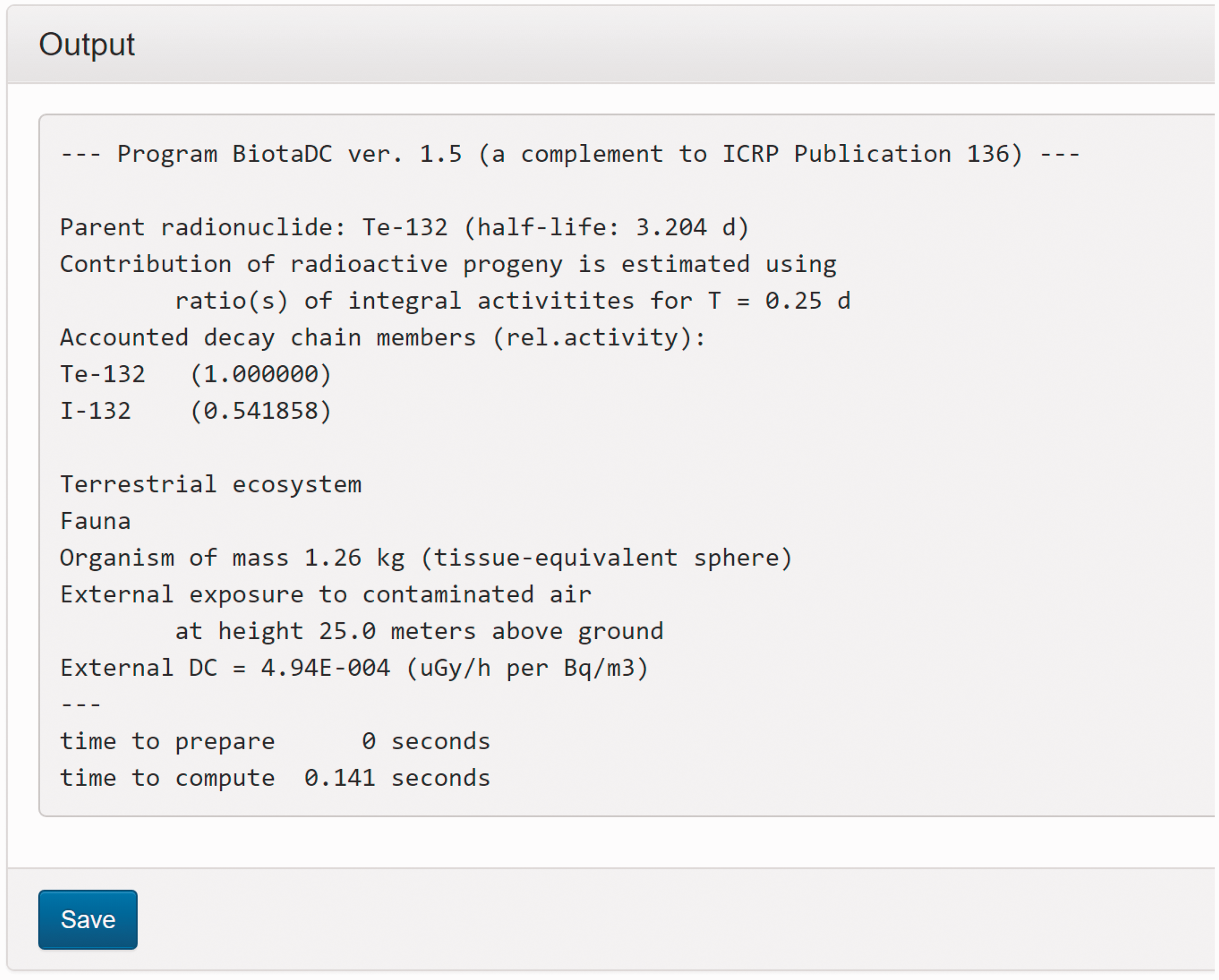
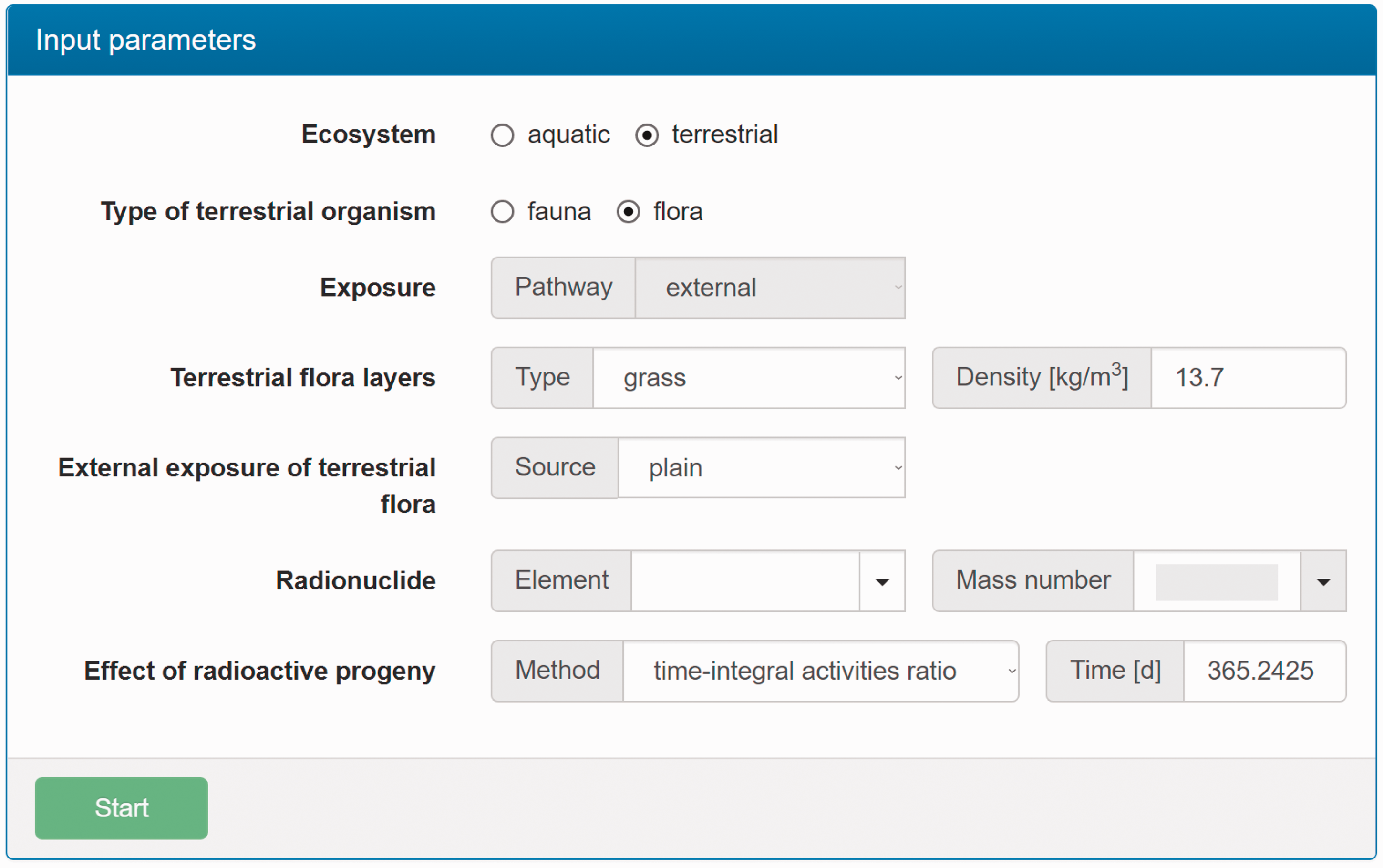
(C5) The programme BiotaDC can be found at the following web address: http://biotadc.icrp.org. After connection to this website, a user sees the following introductory screen (Fig. C.1). At this point, the user should select the ecosystem of interest: aquatic or terrestrial. (C6) If aquatic ecosystem is selected, the user is provided with an input form to specify required parameters of the organism and the exposure conditions for which the DC should be calculated (Fig. C.2):
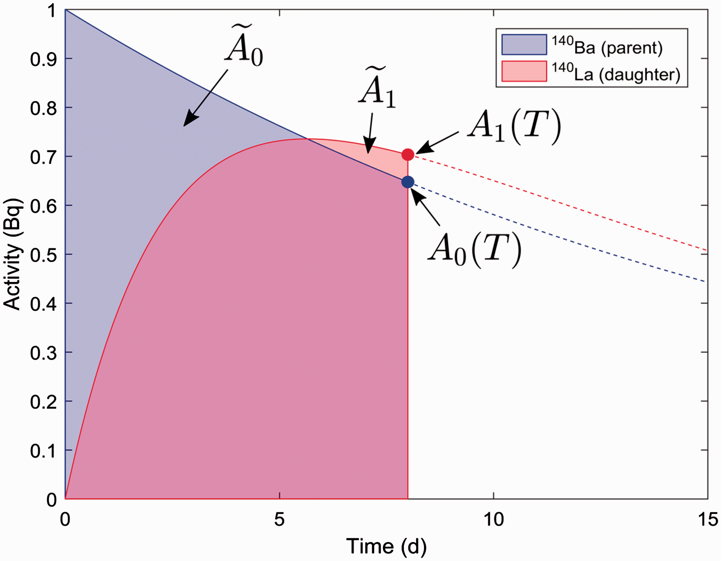
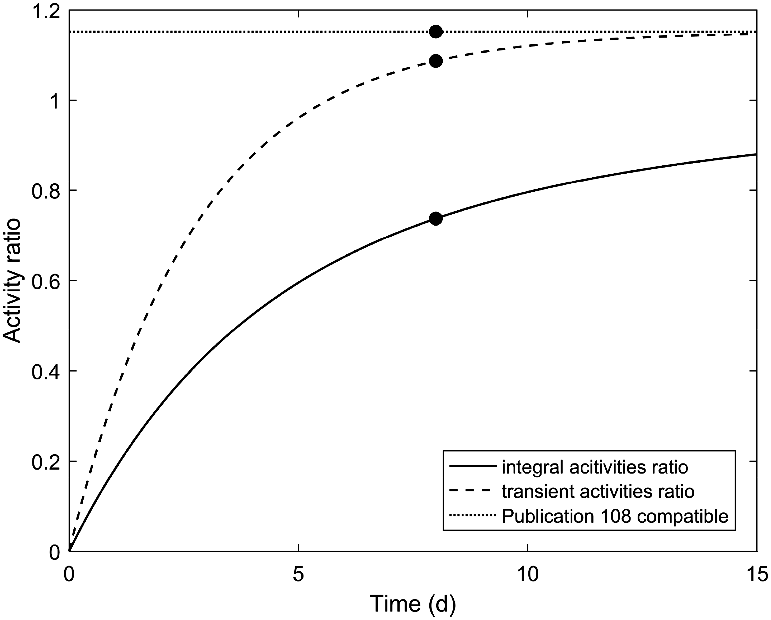
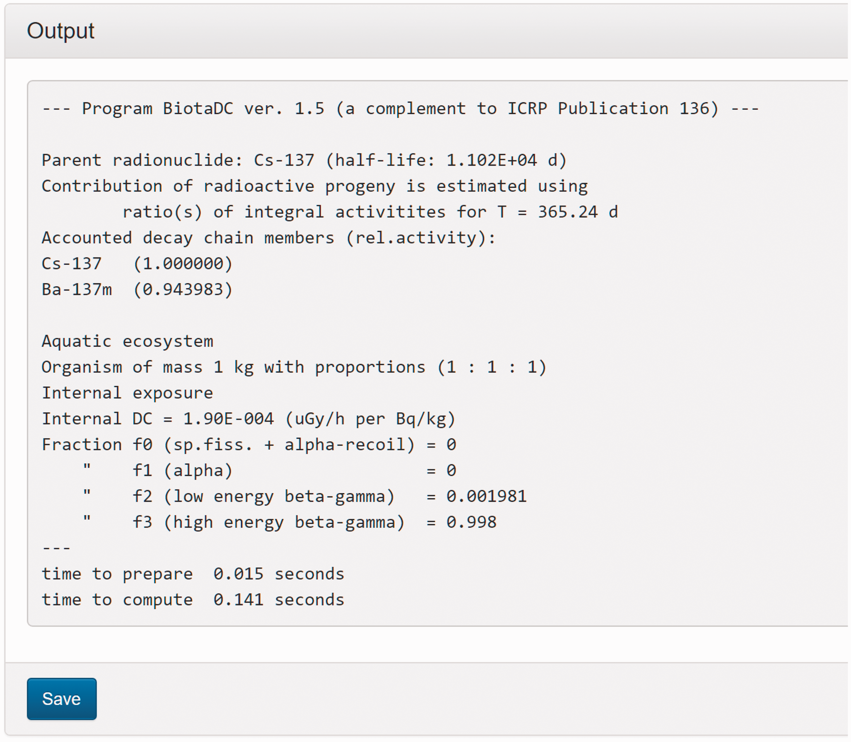
Parameter selection screen for aquatic organisms. exposure pathway: internal or external; body mass within the range from 10−6 to 1000 kg; proportions of the body in the form of relative lengths of axes of an ellipsoid which most reasonably approximates the body shape, assuming the longest axis to be of unit length and lengths of the shorter axes to be in the range from 0 to 1; element and mass number of the radionuclide of interest; and a method to account for radioactive progeny and its characteristic time. (C7) Input of body mass and proportions is fully flexible, and any value within the allowed ranges can be given by the user. For convenience and as a reference, the body masses and proportions of RAPs (ICRP, 2008b) are shown in Table C.1, as required for input in the programme. Shown in Table C.1 are the lifetimes of the RAPs, which can be found helpful for selection of appropriate time constants when considering the effect of radioactive progeny in decay chains. (C8) The methods of accounting for radioactive progeny are illustrated in Figs C.3 and C.4 using the simplest ‘parent + daughter’ decay chain of 140Ba ( The ‘time-integral activities ratio’ (default) indicates a recommended method to account for the contribution of radioactive progeny to the DC. Energy emitted by the daughter nuclides is added to the parent contribution using relative weights based on time-integrated activities of the parent and the daughters, assuming no daughters at the beginning of the parent decay. The time-integral activities of the parent and the daughter nuclides are shown as shaded areas The ‘transient activities ratio’ method can be used to choose an alternative method of accounting for the daughters’ contributions, when transient activities of the decay chain members at a time, defined by the input parameter ‘time’, after the beginning of the parent decay are used to calculate relative weights of the decay chain members. The transient activities are shown as curves and points ‘Publication 108 compatible’ denotes the method compatible with that used in Publication 108 (ICRP, 2008b) and in the ERICA tool (Brown et al., 2008). Namely, DCs include contributions from the parent radionuclide and from the daughters in the truncated decay chain under the assumption of equilibrium activity ratios (shown by the dotted curve in Fig. C.4). The decay chain is truncated at the first daughter nuclide for which the physical half-life is >10 days, or longer than the physical half-life of the parent nuclide. For this method, the truncation time is a fixed parameter equal to 10 days, so input of the parameter ‘time’ is not allowed and the corresponding input field is disabled. (C9) When all parameters have been specified (Fig. C.2), pressing the ‘start’ button results in output as shown in Fig. C.5. The output listing shows the parent radionuclide, information on the option used to calculate contributions from the decay chain members, a list of the radionuclides in the decay chain along with their relative activities used for DC calculation, ecosystem, organism properties (body mass and proportions), type of exposure (internal), DCs for external or internal exposures, relative fractions of internal DC due to various types of radiation, and run times. (C10) Alternatively, selection of the terrestrial ecosystem will result in the following screen (Fig. C.6), where the type of terrestrial organism needs to be specified to show other elements of the input interface. (C11) Selection of ‘fauna’ and ‘internal’ exposure pathway results in the input form (Fig. C.7) similar to that for aquatic organisms with the same input fields. (C12) If, however, for terrestrial organisms, selections are made for ‘fauna’ and ‘external’ exposure, the input form changes (Fig. C.8) and does not show any means to specify proportions of the organism’s body. This is due to the current model for external exposure of terrestrial organisms that provides a dosimetric response for spherical bodies. Additional parameters shown in the input form in this case are the type of environmental radiation source and the organism’s height above the ground surface. (C13) An example of the results of DC calculations after selecting external exposure for terrestrial organisms is shown in Fig. C.9. Here, external DCs have been calculated for a bird with body mass of 1.26 kg (e.g. Reference duck) at height 25 m above the ground flying through air contaminated by 132Te. The contribution of the short-lived daughter 132I is accounted for using relative weights calculated from activities integrated within a 6-h period. (C14) Finally, Fig. C.10 shows the parameter input form if external exposure of terrestrial flora has to be calculated using the simple model of homogeneous vegetation layers. Time-dependent activity of 140Ba (parent) and 140La (daughter) following radioactive decay of 1 Bq of 140Ba. Time-dependent ratios of integral (solid line) and transient (dashed line) activities of 140La (daughter) and 140Ba (parent) in comparison with equilibrium activity ratio (dotted line) implied in the dose coefficients of Publication 108 (ICRP, 2008b). Output after specifying input parameters as shown in Fig. C.2. Parameter selection screen for terrestrial organisms. Type of organism is not yet specified. Parameter selection screen for terrestrial organisms. Fauna has been selected. Parameter selection screen for terrestrial animals. External exposure above the ground surface to radioactively contaminated air has been selected. Results of calculation for the case shown in Fig. C.8. Parameter selection screen for terrestrial organisms. Flora has been selected.