Detecting uniform differential item functioning for continuous response computerized adaptive testing

Abstract

Evaluating items for potential differential item functioning (DIF) is an essential step to ensuring measurement fairness. In this article, we focus on a specific scenario, namely, the continuous response, severely sparse, computerized adaptive testing (CAT). Continuous responses items are growingly used in performance-based tasks because they tend to generate more information than traditional dichotomous items. Severe sparsity arises when many items are automatically generated via machine learning algorithms. We propose two uniform DIF detection methods in this scenario. The first is a modified version of the CAT-SIBTEST, a non-parametric method that does not depend on any specific item response theory model assumptions. The second is a regularization method, a parametric, model-based approach. Simulation studies show that both methods are effective in correctly identifying items with uniform DIF. A real data analysis is provided in the end to illustrate the utility and potential caveats of the two methods.

Introduction

Measurement developers often examine the fairness of their instruments by studying their measure’s item-factor relationships across different groups of respondents. Presumably, an individual’s response to an item should depend only on the latent variable(s) the item intends to measure (e.g., understanding scientific principles); it should not depend on other construct-irrelevant person-level characteristics. However, an item is considered to exhibit differential item functioning (DIF) when two of an item’s characteristics differ for different groups of individuals after controlling for overall differences in performance (Holland & Thayer, 1988). Two types of DIF are often differentiated: uniform DIF and non-uniform DIF. The former refers to an item having a constant advantage for a particular group, whereas the latter refers to the advantage varying in magnitude and/or direction across the latent trait continuum (Penfield & Camilli, 2006; Woods & Grimm, 2011). When DIF is found, the validity of the measurement is called into question: the offending item will require further inspection and may need to be removed or revised.

The current operational DIF analysis is predominately based on Mantel and Haenszel (1959) chi-square statistics (MH; Holland & Thayer, 1988), simultaneous item bias test (SIBTEST, Shealy & Stout, 1993; Chang et al., 1996), and an effect size based on the standardized mean difference in item scores across groups (Dorans & Kulick, 1986; Zwick et al., 1993). All these methods are non-parametric as they do not depend on any specific item response theory (IRT) models. However, they are only designed for dichotomously or polytomously scored items, and they are more powerful in detecting uniform DIF than non-uniform DIF (Lei et al., 2006). In CAT where total score is no longer a valid matching criterion, both MH and SIBTEST are modified using latent trait as the matching variable (Nandakumar & Roussos, 1997; Zwick et al., 1994).

Other popular and parametric DIF detection methods are logistic regression (LR) (Swaminathan & Rogers, 1990) and IRT-likelihood ratio test (IRT-LRT; Thissen et al., 1993). LR models item responses as a function of group indicators, trait estimates (denoted by θ), and their interaction. Then it compares a null model (assuming no DIF) on an item to two nested models formed in hierarchy with an explanatory group variable and group-by-θ interaction variable. IRT-LRT, on the other hand, models differences in item parameters between groups conditioning on the invariance of other items in the test (i.e., anchor items), and it can model impact. Both LR and IRT-LRT are adapted in CAT (Lei, et al., 2006) and they show good Type I error control and adequate power.

Recently, a new set of methods for DIF detection starts to emerge in literature, namely, the regularization methods. Regularization is a machine learning technique that imposes a penalty function during estimation to remove parameters that have little influence on the fit of the model (Bauer et al., 2020; Belzak & Bauer, 2020; Magis et al., 2015; Tutz & Schauberger, 2015; Wang et al., 2023). In the context of DIF detection, an item-level DIF parameter is introduced for each covariate and item parameter type. Then a penalty is imposed on the DIF parameters, and with appropriate regularization algorithms, they will either shrink to 0 implying no DIF or remain non-zero implying DIF. The advantage of the regularization method is, compared to other model-based methods reviewed above, that it does not require pre-specifying anchor items. In addition, all these studies have found that the regularization method maintains good Type I error control and reasonably high power even when there is a large proportion of DIF items, whereas LRT usually fails with severely inflated Type I error. However, the regularization methods have not been evaluated in CAT, especially severely sparse CAT.

In addition, although various methods for DIF detection have been broadly discussed and evaluated, these methods cannot readily handle continuous responses. With recent advances in educational measurement that make use of performance-based items, adaptive testing with non-categorical response items (e.g., when the examinee’s performance is rated on a continuous scale between 0 and 1) is becoming more prevalent. Thus, in this article, we propose DIF detection methods designed specifically for assessments that are growingly used in online learning, in which (1) the items are automatically generated and hence the number of total items is exceedingly large; (2) the items are administered adaptively, which means that the examinee will receive a very small subset of all potential items, and as such, there will be a high proportion of missing data/empty person-item cells. The ultra large number of items in the bank along with excessive missingness is in sharp contrast to the small item bank considered in the current scarce literature on the DIF CAT topic (Zwick et al., 1994; Zwick et al., 1993; Lei et al., 2006; Nandakumar & Roussos, 2004), for example, item bank size of 75 items in (Zwick et al., 1994, Zwick et al., 1993); and (3) the type of response will be on a bounded continuous scale (i.e., proportion of successful task completion), rather than the typical binary/polytomous options, or the normally distributed continuous responses that classic factor-analytic models sufficiently handle. In what follows, we will introduce the model for continuous responses, followed by the two proposed DIF detection methods. Then we will present the simulation study and a real data analysis.

Methods

Model Description

An example of a continuous item example is a sentence completion item in an English language assessment. ^{1 .} In this task, the first and last sentences of a text are fully intact, whereas alternating words in the middle sentences are damaged by masking the second half of the word. Test takers need to rely on context and discourse information to reconstruct the damaged words. In this case, while the completion of each word can be scored as right/wrong (i.e., binary), the score for a paragraph is often computed as the proportion of damaged words that are correctly reconstructed. Such a score is a continuous variable bounded between 0 and 1. In Item Response Theory (IRT), the earliest continuous response model (CRM) was proposed by Samejima (1973) as a limiting case of the graded response model. Wang and Zeng (1998) proposed a different parameterization of it. The primary idea is to translate a bounded response $y$ as $z=\log \frac{y}{k-y}$ , where $k$ is the highest score (in the example above, $k=1$ ) such that $z$ is unbounded and assumed to follow a normal distribution. One notable feature of this model is that the item information function is a constant and it equals to the squared discrimination divided by scaling parameter (i.e., dispersion). Hence, if both the discrimination and dispersion parameters are 1 as in a Rasch version model, the item information will be a constant of 1 across the latent trait continuum. That means for items with varying difficulty levels in educational measurement, they all provide the same level of information across the ability/proficiency continuum, and this may not make intuitive sense in certain applications.

While Samejima (1973)’s CRM seems to be appropriate for any type of bounded continuous responses with an arbitrary bound of 0 and $k$ , the beta IRT model proposed by Noel and Dauvier (2007) is specifically for probabilistic agreement items. That is, instead of reporting agreement on a typical 5-point Likert scale, individuals can report their agreement with items by tracing a vertical mark somewhere on a fixed-length segment, with two ends labeled as “0%” and “100%” agreement, respectively. Note that Samejima (1973)’s CRM can only handle responses in an open interval (0, k), whereas the beta IRT model allows responses in the closed interval [0, 1]. Most recently, Molenaar et al. (2022) proposed a most general zero and one inflated IRT model for bounded continuous data, which can accommodate other existing CRMs (e.g., Ferrando, 2002; Mellenbergh, 1994; Thissen et al., 1983). This general model is yet to gain traction in practice partly due to lack of available software for practitioners to easily implement the model on their data sets.

In this article, we use a signed response theory model (SRT; Maris, 2020; Maris & van der Maas, 2012) for two reasons: (1) it is a continuous extension of the Rasch model and hence enjoys a nice property of the Rasch model, that is, the score of an individual is a sufficient statistic of his/her ability. In other words, the response vector $\mathit{Y}$ is independent of ability θ given the scoring rule $S\left(\mathit{Y}\right)$ ; (2) it is simple and therefore convenient in CAT when latent traits need to be estimated on the fly; and (3) the model was used in the real data example that will be described later. Note that studying different continuous response models is not the focus of this study, but instead, our proposed DIF detection method is agnostic to specific models. In fact, the modified CAT-SIBTEST is a model-free method; hence, it can be used on any continuous response models. The Rasch regularization method is built on the SRT but the idea of “regularization” can be applied to other models, see Belzak and Bauer (2020) or Wang et al., 2023.

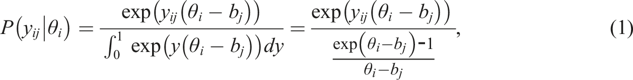
Based on the assumption of sufficient statistics, Maris and van der Maas (2012) derived the SRT that belongs to the exponential distribution. For person $i$ and item $j$ , the density function of a continuous response $y_{ij}$ is as follows

$P\left(y_{ij}|{\theta }_i\right)=\frac{\exp \left(y_{ij}\left({\theta }_i-b_j\right)\right)}{{\int }_0^1\hspace{0.17em}\exp \left(y\left({\theta }_i-b_j\right)\right)dy}=\frac{\exp \left(y_{ij}\left({\theta }_i-b_j\right)\right)}{\frac{\exp \left({\theta }_i-b_j\right)‐1}{{\theta }_i-b_j}},$

(1)where $b_j$ is the difficulty level of item $j$ . Given the known item parameters, the ability ${\theta }_i$ can be estimated by simply maximizing the likelihood constructed from SRT, $l_i\left(\mathrm{\theta }\right)={\displaystyle \sum }_j\log \left(P\left(y_{ij}|{\theta }_i\right)\right)$ , resulting in a maximum likelihood estimate (MLE). Maris (2020) suggested to estimate ${\theta }_i$ by minimizing the cross-entropy (MCE) defined as

$CE\left({\theta }_i\right)={\sum }_j\left[y_{ij}\hspace{0.17em}\log \left(P_i\left(\mathrm{\theta }\right)\right)+\left(1-y_{ij}\right)\log \left(1-P_i\left(\mathrm{\theta }\right)\right)\right]$ , where $P_i\left(\mathrm{\theta }\right)=\frac{1}{1+\exp \hspace{0.17em}‐\left({\theta }_i-b_j\right)}$ is simply the item response function of a Rasch model. Different from the SRT likelihood, minimizing cross-entropy inherently ignores the randomness of the item responses. Our preliminary study reveals that when the item responses are simulated from SRT and when test length is long ( $\ge 10)$ , MLE is more accurate than MCE. However, for shorter test length ( $\le 6$ ), MCE is more accurate.

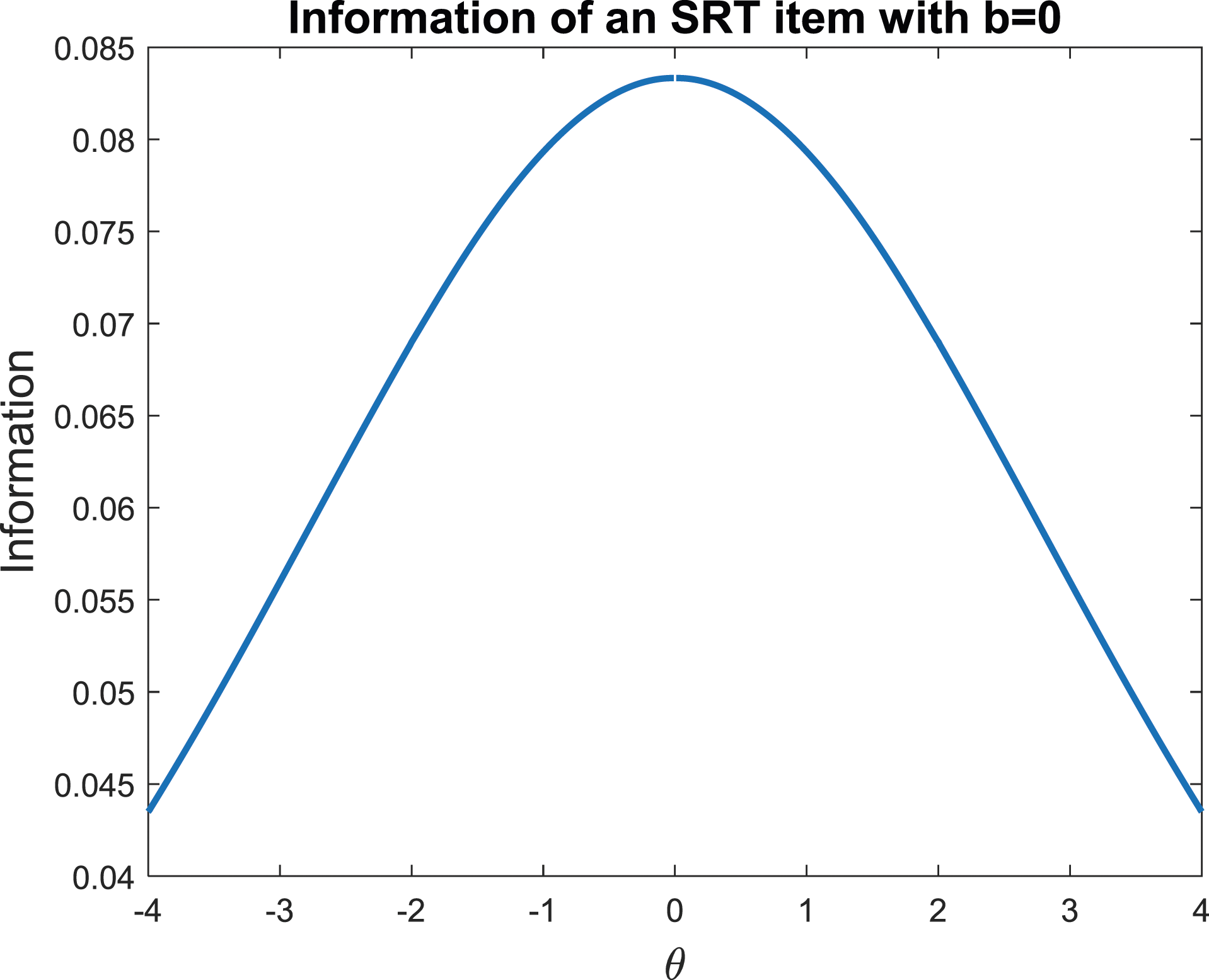
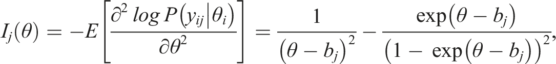
Given the density function defined in Equation (1), the item information function can be derived as follows:

$I_j\left(\theta \right)=-E\left[\frac{{\partial }^2\hspace{0.17em}\mathit{log}\hspace{0.17em}P\left(y_{ij}|{\theta }_i\right)}{\partial {\theta }^2}\right]=\frac{1}{{\left(\theta -b_j\right)}^2}-\frac{\exp \left(\theta -b_j\right)}{{\left(1-\hspace{0.17em}\exp \left(\theta -b_j\right)\right)}^2},$

and the information reaches maximum when $\theta -b_j\approx 0$ . For instance, assume $b_j=0$ without loss of generality, then Figure 1 provides the information curve of this item as a function of $\theta \in \left[-4,4\right]$ . Similar to the Rasch model, the information curve is symmetric, bell-shaped, and reaches maximum when $\theta$ is closest to $b_j$ . Of course, the information is undefined when $\theta =b_j$ , which will rarely happen in practice.

Figure 1.

Illustration of an SRT item information.

Two DIF Detection Methods

We study two uniform DIF detection methods that cover totally different approaches: one is a non-parametric model-free method and the other is a parametric model-based method. The intention is to broaden the scope of the study and the results from the two methods will complement each other. In addition, the following two methods can handle the case when item parameters are provided (such as our real data example) and when there is severe missingness and large item pool due to adaptive design and generative AI. ²

Modified CATSIB Method

This method is an extension of the CATSIB method proposed in Nandakumar and Roussos (2004) to the signed response theory model. As a variant of the SIBTEST, we will first briefly describe the SIBTEST by Shealy and Stout (1993). Let $P_R\left(\theta \right)$ and $P_F\left(\theta \right)$ denote the probabilistic item response on a given item conditional on $\theta$ , where the subscripts R and F refer to reference and focal group, respectively. Item subscript is omitted to avoid clutter. Then DIF on this item at a fixed value of $\theta$ is defined as

$DIF\left(\theta \right)=P_R\left(\theta \right)-P_F\left(\theta \right).$

(2)Then DIF for an item, denoted as $d$ , is defined as the average of $DIF\left(\theta \right)$ over the distribution of $\theta$ , that is

$d=\mathbf{\int }DIF\left(\theta \right)f\left(\theta \right)d\theta ,$

(3)where $f\left(\theta \right)$ denotes a density of $\theta$ based on combined focal and reference groups. Then the null and alternative hypothesis for DIF is $H_0:d=0$ versus $H_a:d\ne 0$ .

For Equation (2) to work, the reference and focal group test takers need to be matched on ability before comparing their performance on the target item. In traditional non-adaptive tests, test takers are matched on their estimated true score from their observed total score, via a so-called regression correction approach (Shealy & Stout, 1993). In CAT, the latent trait estimate $\widehat{\theta }$ serves as a natural matching criterion. To correct for potential impact (i.e., difference in $\theta$ between two groups), Nandakumar and Roussos (2004) also proposed a regression correction approach, which is theoretically equivalent to the regression correction employed in the original SIBTEST. Their method is now modified to be suitable for the continuous scoring rubric used in SRT.

First, the test takers will be matched on ${\widehat{\theta }}^{*}=E_g\left[\theta |\widehat{\theta }\hspace{0.17em}\right]$ , where $\widehat{\theta }$ is the estimated latent trait via MLE, and g is a group indicator (i.e., g = R or F). According to the derivations in Nandakumar and Roussos (2004), we have

$E_g\left[\theta |\widehat{\theta }\hspace{0.17em}\right]=E_g\left[\theta \right]+{\rho }_g^2\left(\widehat{\theta }-E_g\left[\widehat{\theta }\right]\right)\hspace{0.17em}$

(4)where both $E_g\left[\theta \right]$ and $E_g\left[\widehat{\theta }\right]$ are the mean of $\widehat{\theta }$ in group $g$ . ${\rho }_g^2$ is a reliability measure that could be obtained as follows: ${\rho }_g^2=1-\frac{{\sigma }_e^2}{{\sigma }_{\widehat{\theta }}^2}$ . Here ${\sigma }_{\widehat{\theta }}^2$ is the sample variance of $\widehat{\theta }$ in group $g$ , and ${\sigma }_e^2$ is the error variance from the CAT administration. Specifically, in a variable-length CAT, the test often terminates when the standard error of measurement is below a pre-specified cutoff (e.g., Wang et al, 2018). Then ${\sigma }_e^2$ can be obtained as the average squared standard error of $\widehat{\theta }$ at the conclusion of the test.

After obtaining ${\widehat{\theta }}^{*}$ , the estimated DIF from Equation (3) can be approximated as

$\widehat{d}={\sum }_{q=1}^Q\left[{\overline{P}}_R\left({\widehat{\theta }}_q^{*}\right)-{\overline{P}}_F\left({\widehat{\theta }}_q^{*}\right)\right]p\left({\widehat{\theta }}_q^{*}\right),$

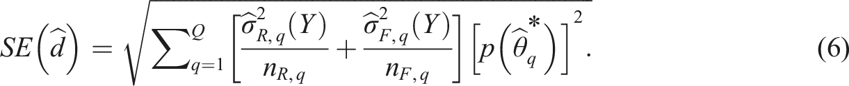
(5)where ${\widehat{\theta }}_q^{*}$ is the $q^{th}$ quadrature point selected from an interval of $\left[-4,4\right]$ . Because ${\widehat{\theta }}^{*}$ is on a real-valued continuous scale, we can divide the observed ${\widehat{\theta }}^{*}$ range into $Q$ equal intervals, and ${\widehat{\theta }}_q^{*}$ is the mean of the $q^{th}$ interval. $p\left({\widehat{\theta }}_q^{*}\right)$ is the observed proportion of reference and focal group test takers in the $q^{th}$ interval. ${\overline{P}}_R\left({\widehat{\theta }}_q^{*}\right)$ is the mean score of people with ability estimate in the $q^{th}$ interval in the reference group, and ${\overline{P}}_F\left({\widehat{\theta }}_q^{*}\right)$ is defined similarly. The standard error for $\widehat{d}$ can be estimated from the observed variance of the item responses in each ability interval, that is

$SE\left(\widehat{d}\right)=\sqrt{{\sum }_{q=1}^Q\left[\frac{{\widehat{\sigma }}_{R,q}^2\left(Y\right)}{n_{R,q}}+\frac{{\widehat{\sigma }}_{F,q}^2\left(Y\right)}{n_{F,q}}\right]{\left[p\left({\widehat{\theta }}_q^{*}\right)\right]}^2}.$

(6)In Equation (6), ${\widehat{\sigma }}_{R,q}^2\left(Y\right)$ is the observed variance of item responses from test takers in the $q^{th}$ interval in the reference group and ${\widehat{\sigma }}_{F,q}^2\left(Y\right)$ is defined similarly. $n_{R,q}$ and $n_{F,q}$ denote the number of test takers in the $q^{th}$ interval in the reference and focal groups, respectively. The null hypothesis of no DIF is rejected if the following test statistic

$B=\frac{\widehat{\beta }}{SE\left(\widehat{\beta }\right)},$

(7)exceeds the $100{\left(1-\frac{\alpha }{2}\right)}^{th}$ percentile or below the $100{\left(\frac{\alpha }{2}\right)}^{th}$ percentile from the standard normal distribution.

As indicated in Nandakumar and Roussos (2004), the number of intervals may affect the performance of the test statistic. First, to ensure stable estimate of mean and variance per interval per group, there must be enough test takers in each interval, say a minimum of 5. If the count is smaller than 5 for certain interval, the cell will be eliminated. On the other hand, if the interval is too coarse, the test statistic will be overly sensitive to impact. Hence, a good balance is needed. Despite of large number of test takers, due to the large number of items and potentially small number of test takers per item, we will start with a reasonably large number of intervals, say, 60, and then monitor how many cells may be eliminated due to getting rid of sparse cells. The number of intervals will decrease gradually until no more than 5% of either the reference or focal group test takers are eliminated.

SRT Regularization Method

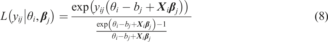
While the modified CATSIB method does not rely directly on estimated items parameters, the regularization method is a model-based parametric method. DIF parameters for an item (i.e., ${\mathit{\beta }}_j$ ) are introduced in the density function of the continuous item response $y_{ij}$ by modifying Equation (1) as follows

$L\left(y_{ij}|{\theta }_i,{\mathit{\beta }}_j\right)=\frac{\exp \left(y_{ij}\left({\theta }_i-b_j+{\mathit{X}}_i{\mathit{\beta }}_j\right)\right)}{\frac{\exp \left({\theta }_i-b_j+{\mathit{X}}_i{\mathit{\beta }}_j\right)-1}{{\theta }_i-b_j+{\mathit{X}}_i{\mathit{\beta }}_j}}$

(8)where ${\mathit{X}}_i$ is a 1-by-P vector including all the grouping information related to DIF for person $i$ . For instance, if we are interested in both gender and first language that may cause DIF, then ${\mathit{X}}_i$ will contain dummy coded information about person’s gender and their first language. ${\mathit{\beta }}_j$ is a P-by-1 vector of regression coefficients implying the effect of grouping variables on item responses. By way of this parameterization, if item $j$ does not have DIF, then ${\mathit{\beta }}_j=0$ .

In contrast to CATSIB in which only two groups are compared at a time, this parameterization allows for simultaneous testing of multiple covariates as well as covariates with more than two levels. For instance, assume first language takes 3 levels: Chinese, Japanese, and Korean. Then $P=2$ in this case such that test takers with Chinese as first language will have ${\mathit{X}}_i=\left(0,0\right)$ , those with Japanese as first language will have ${\mathit{X}}_i=\left(1,0\right)$ , whereas those with Korean as first language will have ${\mathit{X}}_i=\left(0,1\right)$ .

Note that like the multiple-group IRT approach, ${\theta }_i$ in Equation (8) can be written as ${\theta }_{i\left(g\right)}$ to reflect that the distribution of θ is allowed to differ across different groups, hence, it can naturally model impact, if needed. When there are DIF-free anchor items, then depending upon the combination of groups that test takers could be exclusively assigned to, the mean and variance of ${\theta }_{i\left(g\right)}$ for non-reference group could be freely estimated. In this study, we intend to evaluate the comparative performance of this method versus the modified CATSIB method, only pairs of focal/reference groups will be evaluated separately. Therefore, both ${\mathit{X}}_i$ and ${\mathit{\beta }}_j$ become scalars.

During the model estimation, a constrained least absolute shrinkage and selection operator (Lasso; Friedman et al., 2010; Tibshirani, 1996) will be added on the DIF parameter for every item. To perform regularization, we consider two methods: (1) treat everyone’s θ as known from CAT and use conditional likelihood (denoted as “Lasso_Conditional” in the results section); and (2) treat θ as unknown and use marginal log-likelihood (denoted as “Lasso_Marginal”).

In the conditional likelihood method, each ${\beta }_j$ is estimated by maximizing the following objective function

$l\left({\beta }_j\right)={\sum }_{i=1}^{N_j}\hspace{0.17em}\log \hspace{0.17em}L\left({\mathit{Y}}_i|{\theta }_i,{\beta }_j\right)-\lambda \left|{\beta }_j\right|$

(9)where $L\left({\mathit{Y}}_i|{\theta }_i,{\beta }_j\right)={\prod }_{j}L\left(y_{ij}|{\theta }_i,{\beta }_j\right)$ from Equation (8). This objective function can be maximized using the L-BGFS-B method available in the “optimize” function in the “stats” library of R.

In the marginal likelihood method, the log-marginal likelihood is

$\left(\mathit{\beta },\mathbf{\Delta }\right)={\displaystyle \sum }_{i=1}^{N_j}\mathit{log}\hspace{0.17em}{\int }_{{\mathit{\theta }}_i}L\left({\mathit{Y}}_i|{\theta }_i,X_i,\mathit{\beta }\right)q\left({\theta }_i|\mathbf{\Delta }\right)d{\theta }_i-\lambda {\sum }_j\left|{\beta }_j\right|,$

(10)where $\mathbf{\Delta }$ denotes the set of mean and variance of θ if they are estimable, and $N_j$ denotes the number of individuals who answer item $j$ . $L\left({\mathit{Y}}_i|{\theta }_i,\mathit{\beta },\mathbf{\Delta }\right)$ is the likelihood function for person $i$ , and $q\left({\theta }_i\right)$ is the density of θ. A non-zero ${\beta }_j$ for item j implies that this item exhibits uniform DIF for the focal/reference pair. $\lambda$ is the tuning parameter that controls the magnitude of penalty.

Maximizing the marginal log-likelihood in Equation (10) is not computationally feasible. Instead, we use the expectation-maximization (EM) algorithm proceeding as follows. In the E-step, we construct the conditional expectation of the complete data log-likelihood with respect to θ. Suppose at the $\left(r+1\right)$ th EM cycle, we have

$Q^{r+1}\left(\mathit{\beta },\mathbf{\Delta }\right)=E_{\mathit{\theta }|\mathit{Y},{\mathbf{\Delta }}^{\mathit{r}},{\mathit{\beta }}^r}\left(\log \left(L\left(\mathit{\beta },\mathbf{\Delta }|\mathit{Y},\mathit{\theta }\right)\right)\right)\equiv {\sum }_{j=1}^J{Q}_j^{r+1}\left({\beta }_j\right)+Q^{r+1}\left(\mathbf{\Delta }\right)$

(11)where

$Q_j^{r+1}\left({\beta }_j\right)={\sum }_{g=1}^G{\sum }_{i=1}^{N_{gj}}\int \log \hspace{0.17em}L\left({\beta }_j|{\mathit{Y}}_i,\theta ,b_j\right)h\left(\theta |{\mathit{Y}}_i,\mathit{b},{\mathit{\beta }}^r\right)d\theta ,$

(12)where $h\left(\theta |{\mathit{Y}}_i,\mathit{b},{\mathit{\beta }}^r\right)$ is the posterior density of $\theta$ given the current estimate of ${\mathit{\beta }}^r$ and other known information. G denotes total number of groups, and in our case, G = 2, $N_{gj}$ is the number of people in each group who answers item $j$ . $Q^{r+1}\left(\mathbf{\Delta }\right)$ is an integration of normal density with unknown mean ${\mathrm{\mu }}_g$ and variance ${\sigma }_g^2$ .

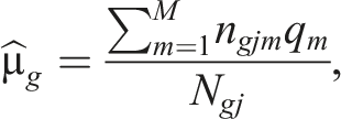
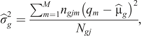
In the M-step, ${\mathrm{\mu }}_g$ and ${\sigma }_g^2$ will be updated using the following closed forms

${\widehat{\mathrm{\mu }}}_g=\frac{{\sum }_{m=1}^M{n}_{gjm}{q}_m}{N_{gj}},$

${\widehat{\sigma }}_g^2=\frac{{\sum }_{m=1}^M{n}_{gjm}{\left(q_m-{\widehat{\mathrm{\mu }}}_g\right)}^2}{N_{gj}},$

where $n_{gjm}={\sum }_{i=1}^{N_{gj}}h\left(q_m|{\mathit{Y}}_i,\mathit{b},{\mathit{\beta }}^r\right)$ is the expected number of persons in group $g$ and $m$ th quadrature bin who answers item $j$ . $q_m$ is the $m$ th quadrature along the θ scale. For the item DIF parameters, ${\beta }_j$ , we can optimize it for different items separately, that is

${\beta }_j=\max \hspace{0.17em}\{Q_j^{r+1}\left({\beta }_j\right)-\lambda \left|{\beta }_j\right|\},$

(13)where $Q_j^{r+1}\left({\beta }_j\right)$ defined in Equation (11) will be numerically approximated by $Q_j^{r+1}\left({\beta }_j\right)={\sum }_{g=1}^G{\sum }_{m=1}^M{n}_{gjm}\hspace{0.17em}\log \hspace{0.17em}L\left({\beta }_j|{\mathit{Y}}_i,q_m,b_j\right)$ . Again, because this is a univariate optimization problem, the L-BGFS-B method available in the “optimize” function will be used.

To find an appropriate value of tuning parameter $\lambda$ in Equation (12) and Equation (13), the Bayesian information criterion (BIC) is applied. We repeat parameters estimating process with different values of $\lambda$ . Each $\lambda$ value will give us an estimate of $\left(\mathit{\beta },\mathbf{\Delta }\right)$ . For the conditional likelihood method, the formula of BIC is given by

$BIC=-2\hspace{0.17em}\log \hspace{0.17em}L\left(\mathit{Y}|\mathit{\beta },\mathit{\theta }\right)+{\Vert \mathit{\beta }\Vert }_0\hspace{0.17em}\log \hspace{0.17em}{N}^{*}$

(14)For the marginal likelihood method, we calculate a log-marginal likelihood for BIC that can be written as

$BIC=-2\hspace{0.17em}\log \int P\left(\mathit{Y}|\mathit{\theta },\mathit{X},\mathit{\beta }\right)q\left(\mathit{\theta }|\mathbf{\Delta }\right)d\mathit{\theta }+{\Vert \mathit{\beta }\Vert }_0\hspace{0.17em}\log \hspace{0.17em}{N}^{*}$

(15)In Equation (14), the first term is −2 times log-marginal likelihood of the observe data and the second term is the $L_0$ norm of $\mathit{\beta }$ estimates times log sample size $N^{*}$ . In CAT, different items tend to have different exposure rate, so there are many choices of $N^{*}$ . Here we take $N^{*}$ = $\min \left(N_j\right)$ , which is the minimum of sample size in responses of all items. The model with the smallest BIC will be selected.

Simulation Study

Design

A simulation study was designed to evaluate the performance of the proposed two differential item function (DIF) detection methods in manipulated conditions imitating our real data example. The sample size was fixed to be 20,000, and item bank was fixed at 1000. True item difficulty, the b parameter, was generated from a uniform distribution, U (-2, 2). This was to mimic the real data, in which the item difficulties followed a near uniform distribution, and again, like real data, the range was chosen to cover the main range of θ′s. We assumed one reference and one focal group, with 50% of the sample in each group. Three DIF factors were manipulated: proportion of DIF items (1%, 5%, and 10%), DIF magnitude, and impact. Three small proportions were considered because of the large item bank of CAT. For DIF magnitude, the $b$ parameter for the studied items in the focal group was set to .25 (small DIF), .50 (medium DIF), or 1.00 (large DIF) higher than the reference group (e.g., Oshima et al., 1997; Suh & Cho, 2014). Only uniform DIF was considered. The trait variable for the focal and reference groups was generated as $\theta \sim N\left(\mu ,1\right).$ We also considered a no-impact and impact scenario. In the conditions of no impact, both focal and reference groups had $\mu =0$ . In the conditions where impact exists, the reference group still had $\mu =0$ , and the mean of θ for the focal group was set to .5. Altogether, there are 18 manipulated conditions. Each condition was simulated for 25 replications. ³ To simulate continuous responses $y_{ij}$ for person $i$ and item $j$ from SRT, we used the inverse-cumulative distribution function (CDF) method, where the CDF of $y_{ij}$ follows $F\left(y\right)=\frac{\exp \left(y\left({\theta }_i-b_j\right)\right)-1}{\exp \left({\theta }_i-b_j\right)-1}$ .

During CAT, the first five items were randomly selected, after $\widehat{\theta }$ is obtained, either the match-b that criterion selects the next item whose b-parameter is closest to the current interim $\widehat{\theta }$ was used or random selection was used. Random selection was included just as a reference baseline. Again, to imitate our real data example, variable-length design was considered, and the stopping rule was set as follows: the test stops either when the interim standard error of $\widehat{\theta }$ is below .25 or when the test length reaches a maximum of 100.

Results

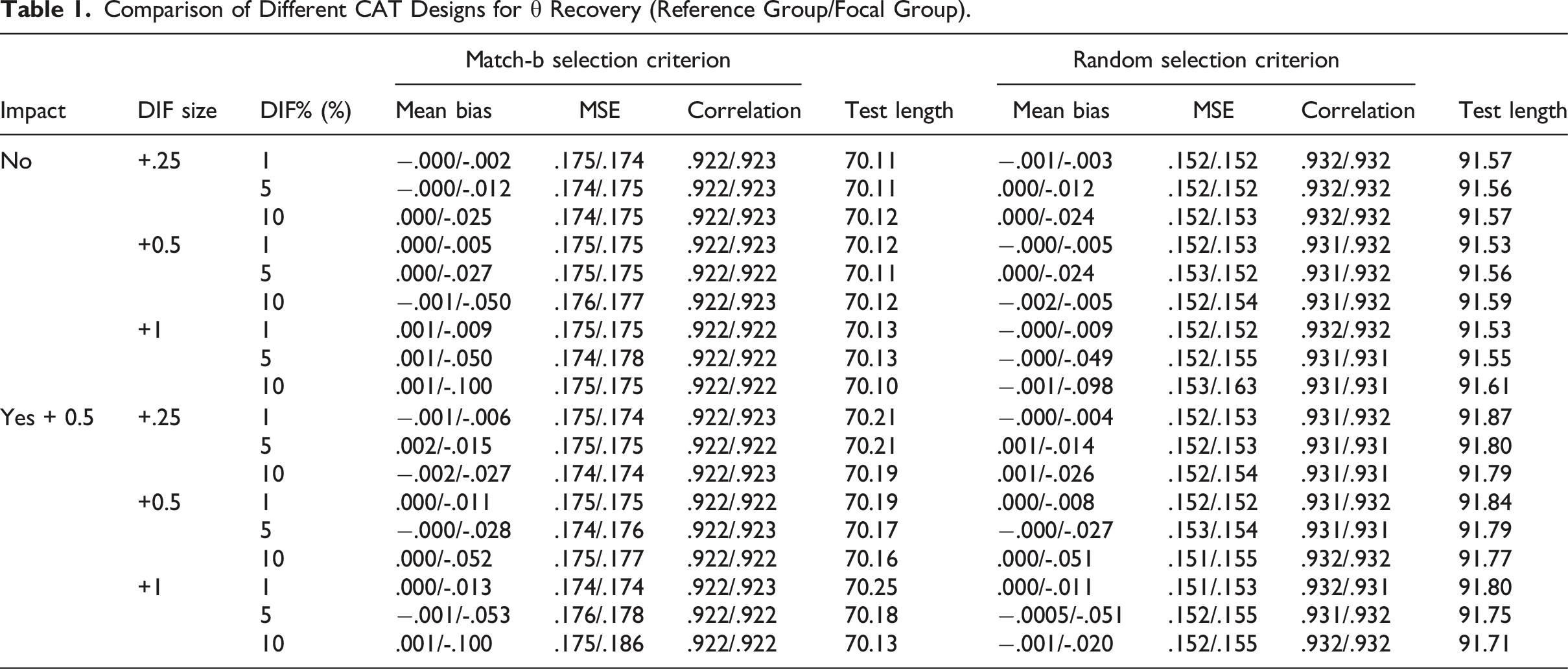
Table 1 displays the θ recovery results for the two item selection criteria under different DIF conditions as a quality control check. As shown, there were no appreciable differences in $\theta$ estimation between different DIF magnitude and DIF proportion conditions. Additionally, having an impact also does not seem to affect $\theta$ recovery much. Overall, match-b item selection seems to produce slightly less accurate $\theta$ estimates in terms of mean bias, RMSE, and correlation. This is merely because the match-b method tends to generate much shorter tests. Hence, we believe the efficiency gain outweigh the little loss of precision.

Table 1.

Comparison of Different CAT Designs for θ Recovery (Reference Group/Focal Group).

Impact	DIF size	DIF% (%)	Match-b selection criterion				Random selection criterion
			Mean bias	MSE	Correlation	Test length	Mean bias	MSE	Correlation	Test length
No	+.25	1	−.000/-.002	.175/.174	.922/.923	70.11	−.001/-.003	.152/.152	.932/.932	91.57
		5	−.000/-.012	.174/.175	.922/.923	70.11	.000/-.012	.152/.152	.932/.932	91.56
		10	.000/-.025	.174/.175	.922/.923	70.12	.000/-.024	.152/.153	.932/.932	91.57
	+0.5	1	.000/-.005	.175/.175	.922/.923	70.12	−.000/-.005	.152/.153	.931/.932	91.53
		5	.000/-.027	.175/.175	.922/.922	70.11	.000/-.024	.153/.152	.931/.932	91.56
		10	−.001/-.050	.176/.177	.922/.923	70.12	−.002/-.005	.152/.154	.931/.932	91.59
	+1	1	.001/-.009	.175/.175	.922/.922	70.13	−.000/-.009	.152/.152	.932/.932	91.53
		5	.001/-.050	.174/.178	.922/.922	70.13	−.000/-.049	.152/.155	.931/.931	91.55
		10	.001/-.100	.175/.175	.922/.922	70.10	−.001/-.098	.153/.163	.931/.931	91.61
Yes + 0.5	+.25	1	−.001/-.006	.175/.174	.922/.923	70.21	−.000/-.004	.152/.153	.931/.932	91.87
		5	.002/-.015	.175/.175	.922/.922	70.21	.001/-.014	.152/.153	.931/.931	91.80
		10	−.002/-.027	.174/.174	.922/.923	70.19	.001/-.026	.152/.154	.931/.931	91.79
	+0.5	1	.000/-.011	.175/.175	.922/.922	70.19	.000/-.008	.152/.152	.931/.932	91.84
		5	−.000/-.028	.174/.176	.922/.923	70.17	−.000/-.027	.153/.154	.931/.931	91.79
		10	.000/-.052	.175/.177	.922/.922	70.16	.000/-.051	.151/.155	.932/.932	91.77
	+1	1	.000/-.013	.174/.174	.922/.923	70.25	.000/-.011	.151/.153	.932/.931	91.80
		5	−.001/-.053	.176/.178	.922/.922	70.18	−.0005/-.051	.152/.155	.931/.932	91.75
		10	.001/-.100	.175/.186	.922/.922	70.13	−.001/-.020	.152/.155	.932/.932	91.71

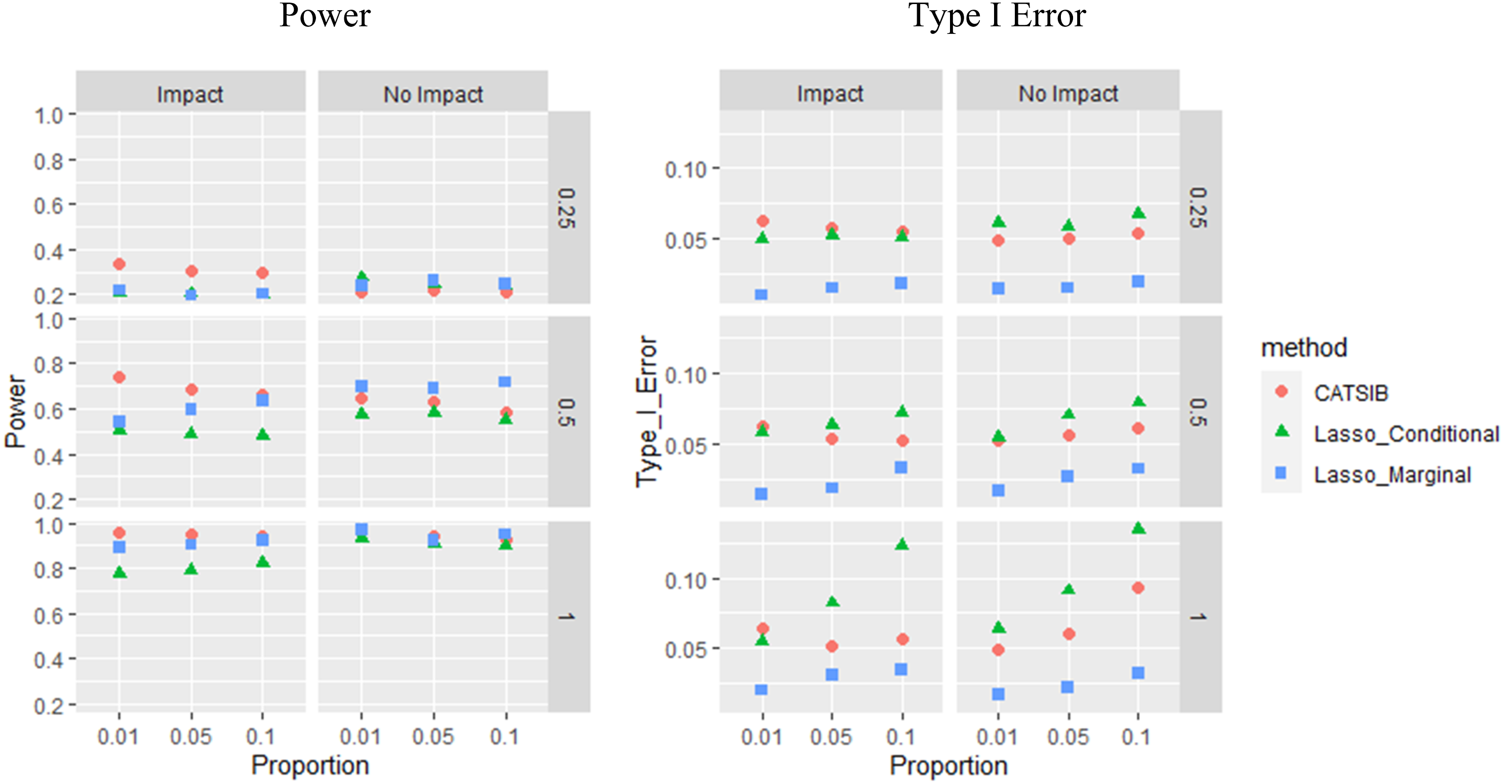
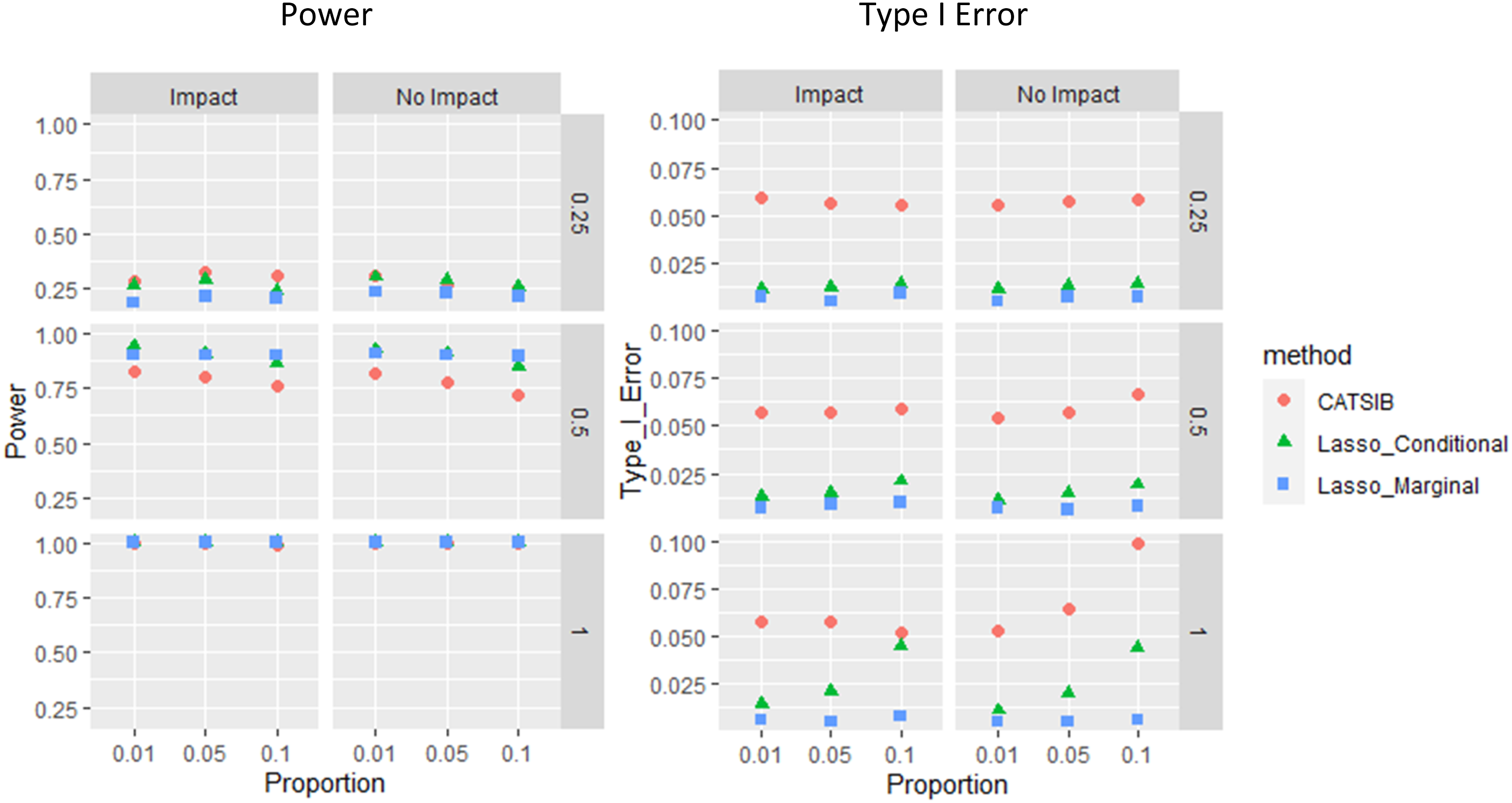
Figures 2 and 3 illustrate the average power (proportion of DIF items correctly detected) and Type I error rate for each condition (proportion of non-DIF items mistakenly flagged), for the match-b CAT design and random selection CAT, respectively. The detailed table results are presented in the Appendix. Within each figure, the three rows include results for the three different levels of DIF magnitude, and the two columns show power and Type I error, respectively.

Figure 2.

Power and type I error of three methods in match-b selection CAT.

Figure 3.

Power and type I error of three methods in random selection CAT.

As can be seen across the figures, for all three methods, increased DIF magnitude led to higher power. In addition, both Type I error and power appeared to be relatively stable with respect to the DIF prevalence, with power dropping slightly when the proportion of DIF items increases. This is understandable in that higher DIF prevalence may lead to slightly biased $\widehat{\theta }$ that will in turn affect the methods that rely on $\widehat{\theta }$ (i.e., CATSIB and conditional Lasso method). It can also be seen that the power for DIF detection in random selection CAT was better than for the match-b selection CAT, which is expected because in random selection CAT, the response data we use to estimate an item’s DIF includes a wider range of trait scores comparative to match-b selection CAT. Indeed, in a typical calibration scenario, heterogeneous sample would also yield more accurate item parameter estimation (e.g., Wang et al., 2020).

For the conditional likelihood lasso method, the estimation of DIF parameter $\mathit{\beta }$ was a simple maximization problem, and since both item difficulty parameter b and latent trait estimates $\widehat{\theta }$ were known, we only needed the data of the focal group to estimate $\mathit{\beta }$ . On the other hand, the marginal likelihood lasso method estimates the latent trait distribution instead of using $\widehat{\theta }$ from CAT. So, it worked stably slightly better than the conditional method across the board.

Although the Lasso with marginal likelihood method shows promising results, its power may be further improved because the current type I errors are very small in all conditions (see Table A1 and A2 in appendix). That means, the information criterion can be further tuned. A drawback of the marginal likelihood method is the computing time. During the estimation, marginal likelihood needs to be calculated in every EM cycle. In the real data application, if match-b item selection CAT is used, conditional likelihood method would be a more economical choice.

A Real Data Example

We obtained a real data set from a variable-length adaptive assessment, which contains 110,260 individuals and each answered 6 items. Each item was scored between 0 and 1 which is exactly our focus of this study: bounded continuous response. There are 3193 items in the bank, and hence the response matrix was quite sparse. To ensure adequate data per item, we used a relatively arbitrary cutoff of 20, that is, we removed 672 items that fewer than 20 individuals answered. Due to the data sparsity and large item bank, instead of using traditional marginal MLE for model calibration, the item difficulty parameters were obtained from large-scale machine-learning–driven language models. They were provided in the data sets, and the mean difficulty is 5.21 and standard deviation is 2.03. Everyone’s ability was also provided, and they were obtained by pooling information from other item types (such as sentence completion test, vocabulary test, etc.) to exploit the potential high correlation among different subdomains of language proficiency. However, as we will explain in detail below, such provided ability estimates (denoted as ${\widehat{\theta }}^p$ where “p” stands for provided) can be used in the modified CATSIB method but not in the regularization method. We first report the modified CATSIB results.

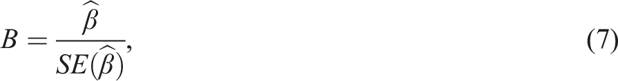
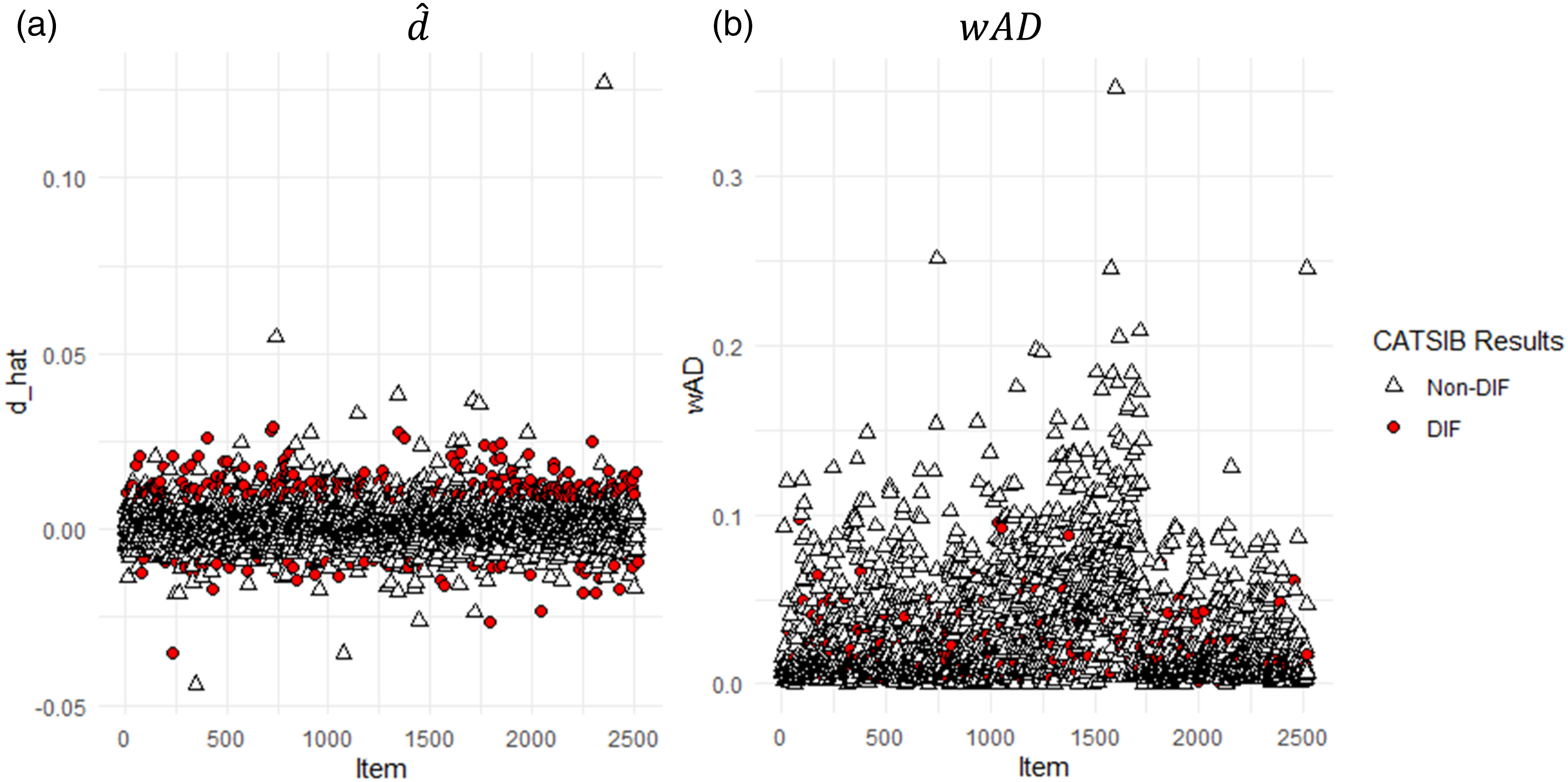
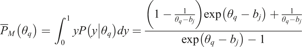
The average ${\widehat{\theta }}^p$ for the male and females are 5.029 and 5.057, respectively, hence, we do not observe much impact existed in the data and therefore, with or without the regression correction in Equation (4) did not seem to make a difference. Figure 4(a) presents each item’s $\widehat{d}$ (i.e., Equation (5)) with color-coded markers to denote detected DIF items versus non-DIF items. Overall, 336 items were flagged to have DIF among 2521 studied items. As shown, the identified DIF items tend to have more extreme $\widehat{d}$ ’s than the non-DIF items. There are a few exceptions, which could be due to their large standard error computed from Equation (6) such that the B-statistic (from Equation (7)) is no longer significantly different from 0. To further validate the DIF detection results, we compute the weighted absolute difference ( $wAD$ ) between the empirical item characteristic curve from the focal and reference group, like the wABC statistics. It is computed as

$wAD=\int \left|P_F\left(\theta \right)-P_R\left(\theta \right)\right|f\left(\theta \right)d\theta \approx {\sum }_q^Q\left|{\overline{P}}_F\left({\theta }_q\right)-{\overline{P}}_R\left({\theta }_q\right)\right|w\left({\theta }_q\right),$

(16)where ${\overline{P}}_F\left({\theta }_q\right)$ and ${\overline{P}}_R\left({\theta }_q\right)$ are the average scores of people in the focal and reference group in the $q$ ^th interval of ${\widehat{\theta }}^p$ . Without imposing any distributional assumptions on θ, we considered $f\left(\theta \right)$ as an empirical density of the $\theta$ distribution in the sample, that is, from a pre-specified interval of −4 to 4 that covers all data in the sample, we used a grid of .2 and counted the proportion of sample falling into each interval. As shown in Figure 4(b), although the detected DIF items had relatively large $wAD$ , there are quite many items with seemingly large $wAD$ that were not flagged. This finding implies that some items may exhibit non-uniform DIF, whereas the current modified CATSIB can only detect uniform DIF.

Figure 4.

Descriptive statistics ( $\widehat{d}$ and $wAD$ ) of DIF and non-DIF items differentiated by the modified CATSIB method. (a) $\widehat{d}$ (b) $wAD$ .

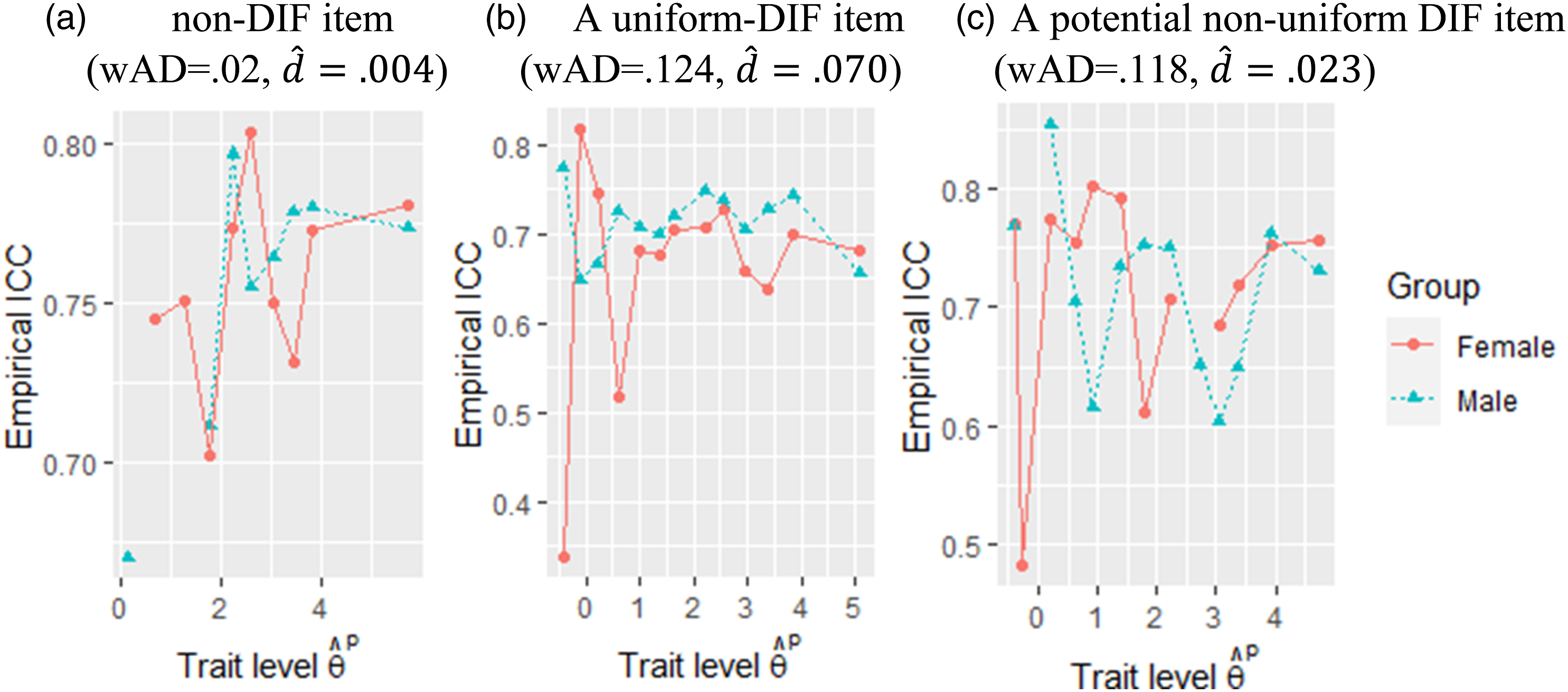
To further verify our detection results and conjecture about the existence of non-uniform DIF, we plot empirical item characteristic curve (ICC) per group for each item. Figure 5 presents the empirical ICC for three representative items, each of which has a sample size larger than 28 per group. Specifically, Figure 5(a) is a DIF-free item with a small $wAD$ and a small $\widehat{d}$ ; Figure 5(b) is an item that is flagged as DIF by the modified CATSIB method, with a large $wAD$ and a large $\widehat{d}$ ; Figure 5(c) is an item that is not flagged (i.e., small $\widehat{d}$ ) but it still has a large $wAD$ , and apparently the two ICCs cross.

Figure 5.

Empirical ICCs per group for three representative groups. (a) non-DIF item (wAD = .02, $\widehat{d}=.004$ ) (b) A uniform DIF item (wAD = .124, $\widehat{d}=.070$ ) (c) A potential non-uniform DIF item (wAD = .118, $\widehat{d}=.023$ ).

With the absence of impact, we also expect the conditional and marginal regularization methods to perform similarly. However, note that the performance of the regularization method depends heavily on the model data fit. Hence, we first computed the weighted absolute difference between model predicted and empirical ICCs, denoted as $ICC\hspace{0.17em}wAD$ . Given that the provided ${\widehat{\theta }}^p$ was computed from an aggregate model that is different from SRT, it would be unfair to use ${\widehat{\theta }}^p$ for evaluating the fit of SRT. Instead, we consider two ways of estimating estimate individual person’s $\widehat{\theta }$ : (1) minimum cross-entropy (MCE; Maris, 2020) ⁴ and (2) MLE. In particular, $\widehat{\theta }$ from the MCE method is used for the conditional Lasso method because it tends to be more accurate when test length is short, whereas $\widehat{\theta }$ from MLE is used to compute $wAD$ for the marginal Lasso method because we need to use a proper likelihood (i.e., SRT model likelihood, note that negative cross-entropy is not a likelihood) in the marginal Lasso method. After computing $\widehat{\theta }$ , we calculate $ICC\hspace{0.17em}wAD$ for each item as follows, and smaller value indicates better item-level model data fit

${ICC\hspace{0.17em}wAD}_j=\int \left|P_M\left(\theta \right)-P_E\left(\theta \right)\right|f\left(\theta \right)d\theta \approx {\sum }_q^Q\left|{\overline{P}}_M\left({\theta }_q\right)-{\overline{P}}_E\left({\theta }_q\right)\right|w\left({\theta }_q\right),$

(17)where $f\left(\theta \right)$ is an empirical density function defined the same as in Equation (16). ${\overline{P}}_M\left({\theta }_q\right)$ is the model predicted average score for people in the $q$ ^th interval, which is computed as follows for the marginal Lasso method (i.e., from SRT model)

${\overline{P}}_M\left({\theta }_q\right)={\int }_0^{1}yP\left(y|{\theta }_q\right)dy=\frac{\left(1-\frac{1}{{\theta }_q-b_j}\right)\exp \left({\theta }_q-b_j\right)+\frac{1}{{\theta }_q-b_j}}{\exp \left({\theta }_q-b_j\right)-1}$

where $P\left(y|{\theta }_q\right)$ is the density function defined in Equation (1). ${\overline{P}}_E\left({\theta }_q\right)$ are the empirical, average scores people in the $q$ ^th interval received. ${\overline{P}}_M\left({\theta }_q\right)$ is computed directly from Rasch model, that is, $\frac{1}{1+\exp \left(-\left({\theta }_q-b_j\right)\right)}$ , for the conditional Lasso method.

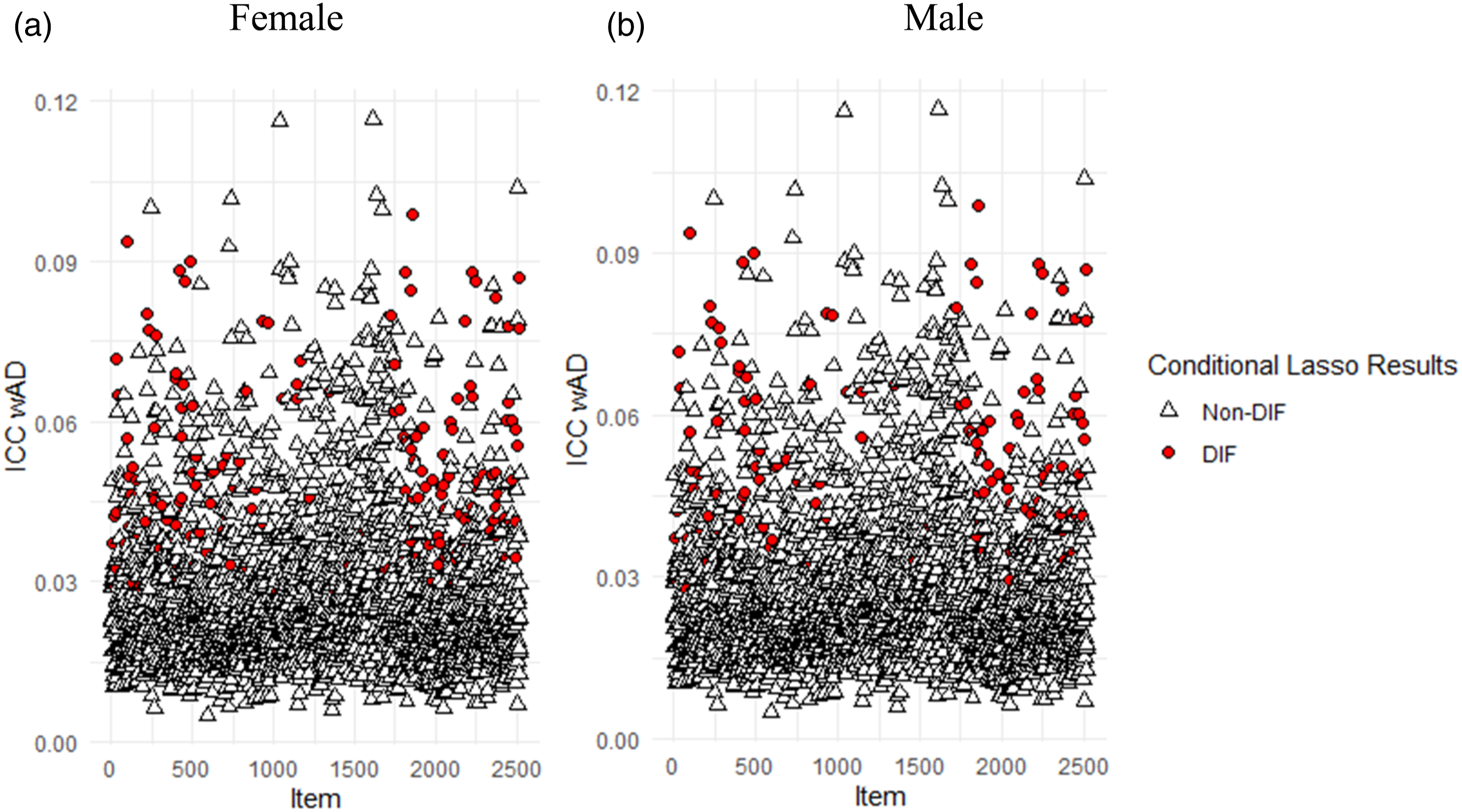
We first conducted the conditional Lasso method conditioning on the MCE estimated $\widehat{\theta }$ . Note that in this method, only data from focal group contributes to the estimation of ${\mathit{\beta }}_j$ (see Equation (8)). Hence, treating either male and female as focal group may or may not yield different results. To exercise due diligence, we ran both and found that the overlap of flagged items is as high as .79. This is interesting as it implies that these flagged items are the items that tend to not fit well with the ICCs defined by the Rasch model, that is, the DIF detection is contaminated by the lack of item fit. Indeed, Figure 6 presents the ${ICC\hspace{0.17em}wAD}_j$ results for both the detected DIF and non-DIF items. As shown, the flagged DIF items tend to have larger ${ICC\hspace{0.17em}wAD}_j$ .

Figure 6.

${ICC\hspace{0.17em}wAD}_j$ for DIF and non-DIF items (detected by the conditional Lasso method) using female (left) and male (right) as focal group. Female (b) male.

Taking female as the focal group as in the CATSIB method, 166 items were flagged as DIF. However, the overlap of detection between the conditional Lasso and the modified CATSIB method is only .127. Like Figure 4, Figure 7 presents ⁵ the $\widehat{d}$ and $wAD$ from those DIF and non-DIF items, and as shown, those flagged items are not necessarily the ones with larger $\widehat{d}$ or large $wAD$ , indicating that the DIF detection in this case is confounded with detection of lack of fit.

Figure 7.

Descriptive statistics ( $\widehat{d}$ and $wAD$ ) of DIF and non-DIF items differentiated by the conditional Lasso method. (a) $\widehat{d}$ (b) $wAD$ .

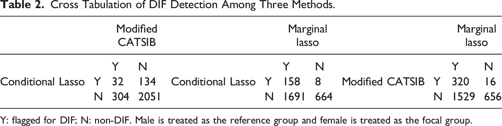
For the marginal Lasso method, although data from both focal and reference group were used for estimation, we still tried both ways of treating female and male as focal groups, respectively, and found the overlap of detected DIF items is as high as .974. Further, we used female group as the focal group as before, 1849 items were flagged as DIF. Interestingly, 158 out of 166 DIF items detected by the conditional Lasso method were flagged again by this method, although the marginal Lasso method flagged many more items. Table 2 presents the cross tabulation of the detected DIF items among the three methods. First, the detection results between the conditional Lasso and modified CATSIB method are largely consistent. Only 32 items (1.26%) out of 2521 are flagged as having DIF by both methods.

Table 2.

Cross Tabulation of DIF Detection Among Three Methods.

		Modified CATSIB				Marginal lasso				Marginal lasso
		Y	N			Y	N			Y	N
Conditional Lasso	Y	32	134	Conditional Lasso	Y	158	8	Modified CATSIB	Y	320	16
	N	304	2051		N	1691	664		N	1529	656

Y: flagged for DIF; N: non-DIF. Male is treated as the reference group and female is treated as the focal group.

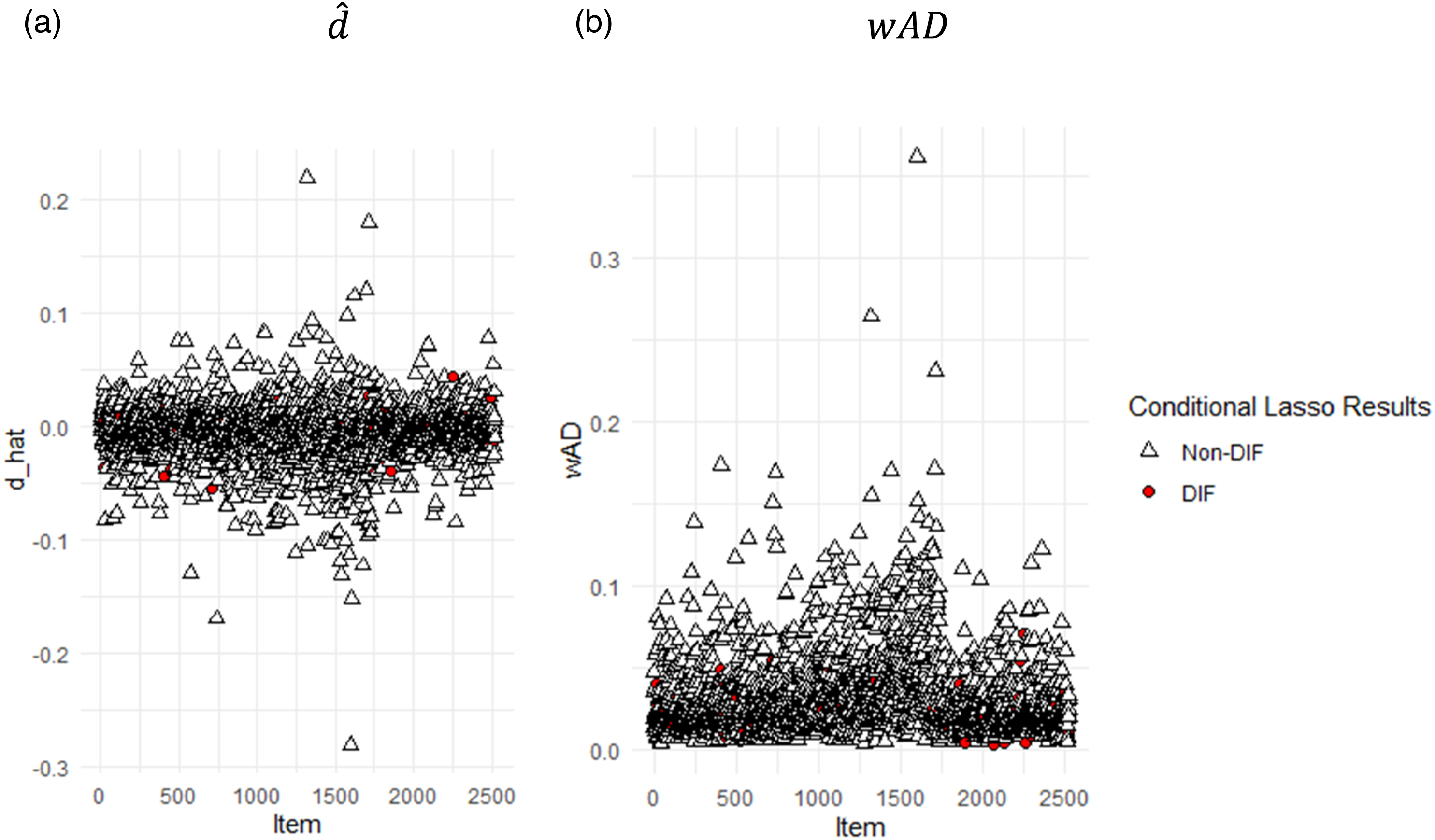
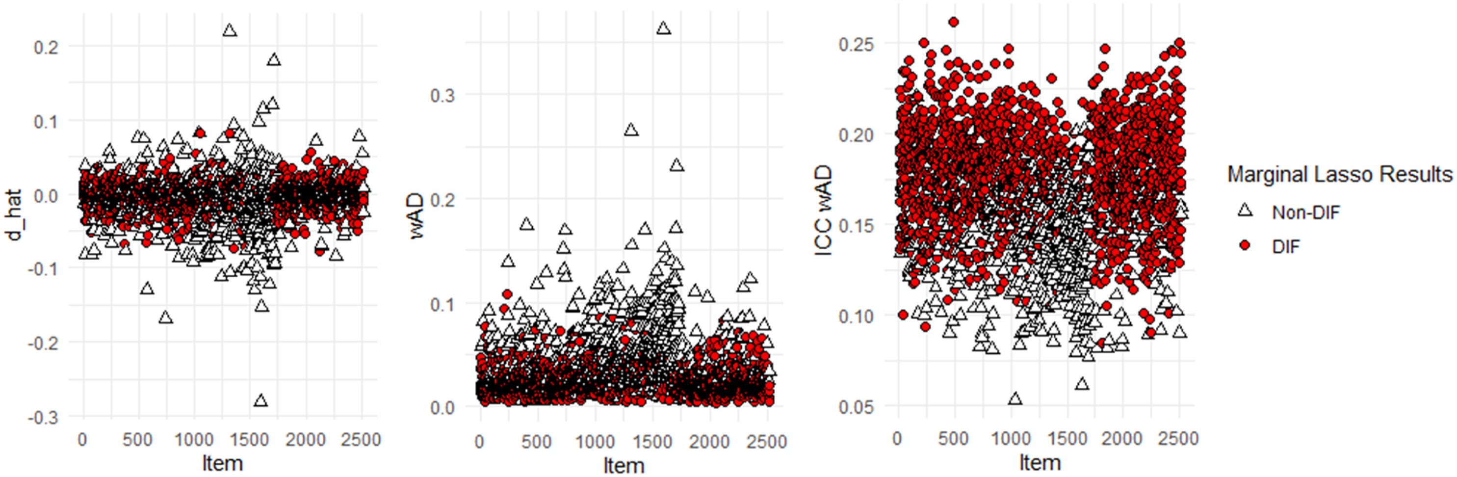
Figure 8 presents the $\widehat{d}$ , $wAD$ , and $ICC\hspace{0.17em}wAD$ computed based on SRT MLE of $\widehat{\theta }$ . As shown, neither $\widehat{d}$ nor $wAD$ appeared to be large for the flagged DIF items, but surprisingly, $ICC\hspace{0.17em}wAD$ tended to separate DIF and non-DIF items well. This reinforces our conjecture that the detected “DIF” items are those that show lack of fit.

Figure 8.

Descriptive statistics ( $\widehat{d}$ and $wAD$ and ICC $wAD$ ) of DIF and non-DIF items differentiated by the marginal Lasso method.

Our real data analysis is somewhat constrained by the SRM because the item difficulty parameters were not directly calibrated from CAT response matrix, but they were from the large language models instead. Relaxing equal discrimination would not be straightforward due to severe sparsity in the response matrix. Hence, future research is needed to allow robust calibration of SRT or other bounded continuous response models directly from the very sparse data.

Discussion

In this arrticle, we extended the CATSIB and regularization methods to detect DIF in continuous, severely sparse CAT. Indeed, the rapidly expanding role of machine learning and artificial intelligence technologies in educational and psychological measurement spur a new genre of assessment which uses “machine learning” techniques to automatically generate items. Such a high-quality, large item pool greatly enables personalized assessment via state-of-the-art variable-length CAT. However, there is no empirical research on DIF detection in this new, yet booming scenario. Our simulation studies showed that both methods hold great promise in detecting DIF for such data type. Specifically, the conditional Lasso method is recommended if the model fits the data, whereas the modified CATSIB is a viable model-free alternative otherwise. The marginal Lasso method, although is statistically optimal in theory and tends to perform the best in simulations, it may be computationally too expensive to apply in practice.

The real data example sheds further light on the application potential of the two methods. That is, the modified CATSIB method appears to be effective to detect items with uniform DIF, although certain effect size measure cutoff can be used in practice to distinguish statistically significant DIF from practically meaningful DIF, such as the standardized mean difference in item scores across groups (Dorans & Kulick, 1986; Zwick et al., 1993). The regularization methods, on the other hand, rely on the adequate model data fit. It appears that those flagged DIF items also tend to be items shown misfit, implying that item misfit may confound with DIF detection. This is especially true for conditional Lasso method: because DIF is reflected by non-zero ${\beta }_j$ in Equation (8), and given known $\theta$ , only data from focal group contributes to the estimates of ${\beta }_j$ . Hence, non-zero ${\beta }_j$ could also mean the current SRT model does not fit the data from the focal group well. In fact, if we use the true focal group as the focal group and true reference group as the reference group, we will observe non-zero ${\beta }_j$ ’s for DIF items, and if we reverse the role of focal and reference group, we will observe zero ${\beta }_j$ ’s instead. However, in our analysis, when we used both female and male group as the focal group in the two separate analyses; we noted that almost the same set of DIF items were detected. This reinforces that it may be the lack of fit, rather than DIF, that contributes to the non-zero ${\beta }_j$ ’s. In this case, results from the modified CATSIB method should hold higher credence.

The current study has several limitations, and hence, it can be expanded in a few directions. First, since we considered a “Rasch” version of a continuous response model (i.e., the SRT model) throughout the study, our focus was on the uniform DIF. However, the modified CATSIB method can be further extended to detect non-uniform DIF, such as in Chalmers (2018). The primary idea is to find ${\theta }_c$ at which $P_R\left({\theta }_c\right)-P_F\left({\theta }_c\right)=0$ , that is, the two ICCs cross, and then update Equation (3) as follows

$d={\int }_{\theta <{\theta }_c}\left(P_R\left(\theta \right)-P_F\left(\theta \right)\right)f\left(\theta \right)d\theta +{\int }_{\theta \ge {\theta }_c}\left(P_F\left(\theta \right)-P_R\left(\theta \right)\right)f\left(\theta \right)d\theta .$

(18)

Chalmers (2018) derived a statistic based on Equation (18) which follows a chi-squared distribution. The regularization method can also be extended to detect non-uniform DIF (see Belzak & Bauer, 2020; Wang et al., 2023). Second, other continuous item response model may be considered in addition to SRT, such as Samejima (1973)’s model which assumes the probability of an observed response larger than or equal to a constant follows a normal cumulative distribution function (Zopluoglu, 2013). Samejima (1973)’s model can be viewed as a limiting form of the graded response model, whereas the SRT model considered herein was derived from a sufficient statistic scoring rule. Third, as we note in the real data analysis, model-based parametric DIF detection methods may be confounded with item misfit. Although conceptually, we can argue that when an item has DIF, the model that assumes measurement invariance will not fit the data well, and hence DIF is a form of item misfit, and flagging misfit items as having DIF is certainly not accurate. Hence, operational analysis protocol should start with model/item fit evaluation followed by DIF analysis. Lastly, we want to acknowledge that the DIF detection for bounded continuous responses may be conducted using generalized factor-analytic models with logit or probit transformation, such that off-the-shelf structural equation modeling (SEM) software may be used. Chi-square tests for nested-model comparison are often used within the SEM framework to evaluate measurement invariance.

Supplemental Material

Supplemental Material - Detecting uniform differential item functioning for continuous response computerized adaptive testing

Supplemental Material for Detecting uniform differential item functioning for continuous response computerized adaptive testing by Chun Wang, and Ruoyi Zhu in Applied Psychological Measurement