Sage Journals: Discover world-class research

Abstract

Marginal maximum likelihood estimation (MMLE) is commonly used for item response theory item parameter estimation. However, sufficiently large sample sizes are not always possible when studying rare populations. In this paper, empirical Bayes and hierarchical Bayes are presented as alternatives to MMLE in small sample sizes, using auxiliary item information to estimate the item parameters of a graded response model with higher accuracy. Empirical Bayes and hierarchical Bayes methods are compared with MMLE to determine under what conditions these Bayes methods can outperform MMLE, and to determine if hierarchical Bayes can act as an acceptable alternative to MMLE in conditions where MMLE is unable to converge. In addition, empirical Bayes and hierarchical Bayes methods are compared to show how hierarchical Bayes can result in estimates of posterior variance with greater accuracy than empirical Bayes by acknowledging the uncertainty of item parameter estimates. The proposed methods were evaluated via a simulation study. Simulation results showed that hierarchical Bayes methods can be acceptable alternatives to MMLE under various testing conditions, and we provide a guideline to indicate which methods would be recommended in different research situations. R functions are provided to implement these proposed methods.

Keywords

auxiliary item information Bayesian estimation explanatory item response model graded response model shrinkage estimator small sample size

Introduction

Item response theory (IRT) is a popular methodology for developing and evaluating scales used in educational and psychological research. In IRT, marginal maximum likelihood estimation (MMLE; Bock & Aitkin, 1981) is commonly used for item parameter estimation (Baker & Kim, 2004). Previous research on MMLE has shown that the accuracy and precision of item parameter estimates is acceptable in medium and large sample sizes (e.g., > 500 for graded response models [GRM]; Forero & Maydeu-Olivares, 2009; Reise & Yu, 1990). In small sample sizes, MMLE can struggle with obtaining accurate and precise item parameter estimates, or may not converge at all. Unfortunately, it is not uncommon for researchers to struggle with obtaining medium or large sample sizes. Studies of rare populations (e.g., individuals with Rett syndrome, students with listening fatigue, and individuals with substance use disorders) can make it difficult to obtain more participants. With small sample sizes, alternative methods are required to obtain accurate and precise item parameter estimates with whatever data are available.

Bayesian estimation methods have been used in IRT estimation to increase the accuracy (by reducing the mean squared error) and precision (by reducing the standard error) of item parameter estimates (e.g., Fox, 2010). However, prior research on IRT Bayesian estimation methods are mainly for item response models without auxiliary item information. Mislevy (1988) proposed an empirical Bayes method using auxiliary item information to increase the stability and precision of item location (or difficulty) estimates in Rasch models. The method proposed by Mislevy (1988) is considered “empirical Bayes” because it uses both maximum likelihood estimates and regression estimates (as prior means) to obtain shrinkage estimates using auxiliary item information in three steps. However, the implementation of this three-step empirical Bayes method differs from the one-step implementation of empirical Bayes most commonly performed in the literature. We discuss these differences in the summary and discussion section. Mislevy (1988) used auxiliary item information (i.e., item domain information such as what mathematical operations were required to solve items) to compensate for the lack of information available from persons in a sample size of 150. Auxiliary item information was used by the empirical Bayes method as item covariates grouping similar items together regarding their content, format, or the skills required to solve them. In Mislevy’s (1988) study, using auxiliary item information resulted in a 25% increase in the precision of item location estimates, an increase that otherwise would have required testing approximately 40 additional persons.

One limitation of the empirical Bayes method used by Mislevy (1988) is that the uncertainty of item parameter estimates is ignored, which can result in underestimated standard errors. This underestimation of standard errors is especially problematic with small sample sizes. To incorporate the uncertainty of item parameter estimates, hierarchical Bayes methods can be used. As opposed to empirical Bayes, which uses point priors for item parameters, hierarchical Bayes methods specify prior distributions on item parameters (called “hyper-priors”). Inverse-gamma (ϵ, ϵ) distributions are typically selected as hyper-priors on the variance of item parameters for their conditional conjugacy (having prior and conditional posterior distributions belonging to the same class), which suggests clean mathematical properties. However, Gelman (2006) does not recommend using inverse-gamma (ϵ, ϵ) distributions as noninformative priors, because the resulting inferences when estimating near-zero standard deviations are highly dependent upon the choice of ϵ. In addition, using diffuse priors on the means of prior distributions results in large errors and convergence problems even when informative inverse-gamma distributions on variances (Inverse-gamma ( $1,1$ )) are used in a hierarchical Bayes approach. Instead of inverse-gamma (ϵ, ϵ) distributions, Gelman (2006) recommends using half-t distributions (specifically half-Cauchy when the number of groups is small) on standard deviations as weakly informative and conditionally conjugate priors.

Likert-type rating scales are common in psychological research. The item response model most widely used for modeling rating scales is the GRM (Samejima, 1969). The GRM is popular for being highly flexible in modeling tests where items have unique thresholds (both in number and location for each item). Although Bayesian analysis has been implemented for the GRM (e.g., Curtis, 2010), no previous research has been conducted to apply the empirical Bayes method (as used by Mislevy, 1988) to the GRM or to evaluate the performance of using half-t and half-Cauchy distributions as hyper-priors in a hierarchical Bayes method for the GRM.

The primary purpose of this study is to apply empirical and hierarchical Bayes methods using auxiliary item information to a unidimensional GRM to obtain item parameter estimates with greater accuracy and precision, particularly in small to medium sample sizes. For the purpose of comparing empirical Bayes and hierarchical Bayes, we extend Mislevy’s (1988) empirical Bayes method for a Rasch model to a GRM, which requires to provide new estimation code to be evaluated for a small to medium sample size. The results of the empirical and hierarchical Bayes methods presented for GRM will guide how and when to use the methods when a GRM is applied to Likert-type rating scales, which has not been shown in the literature. Specific research questions this study plans to answer regarding the GRM are as follows: (1a) Among the estimation methods of interest (MMLE, empirical Bayes, and hierarchical Bayes), which method results in the most accurate item parameter estimates in small to medium sample sizes? (1b) Is a hierarchical Bayes method an acceptable alternative to MMLE in small to medium sample sizes when MMLE is unable to achieve convergence? (2) How much is the accuracy of item parameter estimates in small to medium sample sizes increased by using a hierarchical Bayes method with item covariates compared to a hierarchical Bayes method without item covariates? (3) How much is the underestimation of the standard errors of item parameter estimates reduced in small to medium sample sizes by including the uncertainty of item parameter estimates with a hierarchical Bayes method compared to an empirical Bayes method? These research questions will be answered by comparing the results of MMLE, empirical Bayes, and hierarchical Bayes (with and without the use of item covariates) via a simulation study. An additional research goal of this study is to provide R functions for the application of these empirical and hierarchical Bayes methods.

The rest of this paper is structured as follows. First, the GRM with auxiliary item information and the concept of shrinkage estimators is presented. Second, empirical and hierarchical Bayes methods are described. Third, a simulation study is conducted to evaluate the relative performance of the methods described under various simulation conditions. Finally, we conclude with a summary and discussion.

GRM with Auxiliary Item Information

Samejima’s (1969) GRM specifies the conditional cumulative probability of response y_ji for person j (j = 1, …, J) and item i (i = 1, …, I) in category k (k = 0, 1, …, m_i − 1), where m_i is the number of categories for item i, as follows

P (y_{j i} \geq k | θ_{j}) = {\begin{cases} 1 & if k = 0 \\ {logit}^{- 1} [α_{i} (θ_{j} - β_{i, k})] & if 1 \leq k \leq m_{i} - 1, \end{cases}

(1)

where logit⁻¹ denotes the inverse logit link, α_i is an item discrimination parameter, β_i,k is an item threshold parameter, and θ_j is the latent variable.

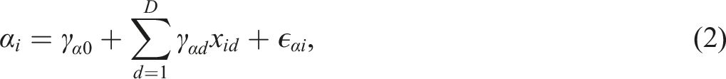
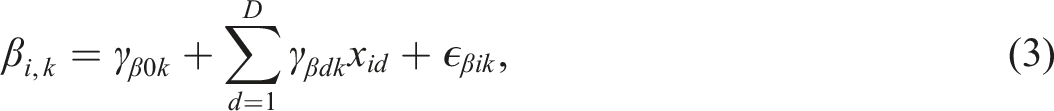
Variability in item parameters across items for a unidimensional test can be explained or predicted using auxiliary item information such as item format, item contents (or domains), or the skills required to solve items (De Boeck & Wilson, 2004). In this paper, we focus on the use of auxiliary item information to obtain stable and precise item parameter estimates of the unidimensional GRM using empirical and hierarchical Bayes methods when there is evidence of unidimensionality in a test. A linear regression model with normal and homoscedastic residuals is assumed for item parameters, as used in other item regression models (e.g., De Boeck, 2008). The regression structure of item discrimination parameters can be imposed as follows

α_{i} = γ_{α 0} + \sum_{d = 1}^{D} γ_{α d} x_{i d} + ϵ_{α i},

(2)

where d is the index for auxiliary item information (or item covariate) (d = 1, …, D), γ_α0 is the intercept parameter, γ_αd is the effect of item covariate x_id on discrimination parameter α_i, and ϵ_αi is the random item residual (random over items), assumed to follow

{(ϵ_{α 1}, \dots, ϵ_{α I})}^{T} \sim N (0, σ_{α}^{2})

, where

σ_{α}^{2}

is the variance of the random item residual. Similarly, for item threshold parameters

β_{i, k} = γ_{β 0 k} + \sum_{d = 1}^{D} γ_{β d k} x_{i d} + ϵ_{β i k},

(3)

where γ_β0k is the intercept parameter, γ_βdk is the effect of item covariate x_id on threshold parameter β_i,k, and ϵ_βik is the random item residual (random over items), assumed to follow

{(ϵ_{β 1 k}, \dots, ϵ_{β I k})}^{T} \sim N (0, σ_{β k}^{2})

, where

σ_{β k}^{2}

is the variance of the random item residual across items for category k.

Methods

In this section, we describe the empirical Bayes and hierarchical Bayes methods implemented in this study, and how these methods can be used to obtain estimates of GRM item parameters by using auxiliary item information. We extend Mislevy (1988)’s empirical Bayes method for the Rasch model to the GRM and then discuss the specification of the prior and posterior distributions for hierarchical Bayes.

Empirical Bayes Method

The estimation of GRM item parameters with an empirical Bayes method takes place over three steps, as described below.

Step 1. Marginal Maximum Likelihood Estimates of Item Parameters

Item parameters (α_i and β_i,k) and corresponding standard errors (τ_αi and τ_βik) were estimated using MMLE to obtain item parameter estimates based on likelihood without prior distributions on item parameters. MMLE was implemented using the mirt package (Chalmers, 2012) in R (R Core Team, 2018).

Step 2. Maximum Likelihood Estimates of the Regression Parameters and the Residual Variance

We consider item regression models (Equations (2) and (3)) using the maximum likelihood estimates of item parameters obtained in Step 1 ( ${\hat{α}}_{i}$ and ${\hat{β}}_{i k}$ ). Because we use the maximum likelihood estimates from Step 1, the uncertainty of these estimates is ignored in Step 2. Maximum likelihood estimates of the regression parameters of these item regression models were obtained using the lm function in R. The regression structure is imposed on item discrimination estimates as follows

{\hat{α}}_{i} = γ_{α 0} + Σ_{d = 1}^{D} γ_{α d} x_{i d} + h_{α i},

(4)

where

{(h_{α 1}, \dots, h_{α I})}^{T} \sim N (0, ϕ_{α}^{2})

. Similarly, for item threshold estimates

{\hat{β}}_{i k} = γ_{β 0 k} + Σ_{d = 1}^{D} γ_{β d k} x_{i d} + h_{β i k},

(5)

where

{(h_{β 1 k}, \dots, h_{β I k})}^{T} \sim N (0, ϕ_{β k}^{2})

. Unbiased estimates of the residual variances (

ϕ_{α}^{2}

and

ϕ_{β k}^{2}

) were calculated using the following equation (Rencher, 2000, p. 143):

{\hat{ϕ}}_{α}^{2} = \sum_{i = 1}^{I} {\tilde{h}}_{α i}^{2} / (I - D - 1)

and

{\hat{ϕ}}_{β k}^{2} = \sum_{i = 1}^{I} {\tilde{h}}_{β i k}^{2} / (I - D - 1)

, where

{\tilde{h}}_{α i}^{2}

and

{\tilde{h}}_{β i k}^{2}

are calculated residuals based on parameter estimates in Equations (4) and (5). In addition, the standard errors of the residual variance for item discrimination estimates and item threshold estimates were calculated using the following equation (Rencher, 2000, p. 143):

{SE}_{ϕ_{α}^{2}} = \sqrt{\frac{2 ϕ_{α}^{4}}{I - D - 1}}

and

{SE}_{ϕ_{β k}^{2}} = \sqrt{\frac{2 ϕ_{β k}^{4}}{I - D - 1}}

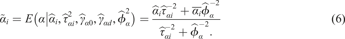
Step 3. Empirical Bayes Estimates of Item Parameters

The empirical Bayes estimates of item parameters and the precision of those estimates are calculated, based on the results obtained from Steps 1 and 2. The empirical Bayes estimate ${\tilde{α}}_{i}$ is the weighted average of the maximum likelihood estimate ${\hat{α}}_{i}$ and the regression estimate ${\bar{α}}_{i} = {\hat{γ}}_{α 0} + Σ_{d = 1}^{D} {\hat{γ}}_{α d} x_{i d}$ with weights proportional to their respective precisions¹

{\tilde{α}}_{i} = E (α | {\hat{α}}_{i}, {\hat{τ}}_{α i}^{2}, {\hat{γ}}_{α 0}, {\hat{γ}}_{α d}, {\hat{ϕ}}_{α}^{2}) = \frac{{\hat{α}}_{i} {\hat{τ}}_{α i}^{- 2} + \bar{α_{i}} {\hat{ϕ}}_{α}^{- 2}}{{\hat{τ}}_{α i}^{- 2} + {\hat{ϕ}}_{α}^{- 2}} .

(6)

Similarly for item threshold parameters, the empirical Bayes estimate ${\tilde{β}}_{i k}$ is the weighted average of the maximum likelihood estimate ${\hat{β}}_{i k}$ and the regression estimate ${\bar{β}}_{i k} = {\hat{γ}}_{β 0 k} + Σ_{d = 1}^{D} {\hat{γ}}_{β d k} x_{i d}$ with weights proportional to their respective precisions

{\tilde{β}}_{i k} = E (β | {\hat{β}}_{i k}, {\hat{τ}}_{β i k}^{2}, {\hat{γ}}_{β 0 k}, {\hat{γ}}_{α d}, {\hat{ϕ}}_{β k}^{2}) = \frac{{\hat{β}}_{i k} {\hat{τ}}_{β i k}^{- 2} + {\bar{β}}_{i k} {\hat{ϕ}}_{β k}^{- 2}}{{\hat{τ}}_{β i k}^{- 2} + {\hat{ϕ}}_{β k}^{- 2}} .

(7)

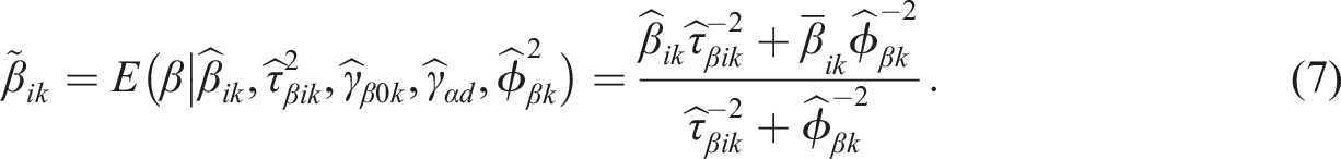
Each empirical Bayes estimate ( ${\tilde{α}}_{i}$ , ${\tilde{β}}_{i k}$ ) gains precision from both the precision of its maximum likelihood estimates ( ${\hat{τ}}_{α i}^{- 2}$ , ${\hat{τ}}_{β i k}^{- 2}$ ) obtained in Step 1 and from the precision of its regression estimates ( ${\hat{ϕ}}_{α}^{- 2}$ , ${\hat{ϕ}}_{β k}^{- 2}$ ) obtained in Step 2: ${\tilde{σ}}_{α i}^{- 2} = {\hat{τ}}_{α i}^{- 2} + {\hat{ϕ}}_{α}^{- 2}$ and ${\tilde{σ}}_{β i k}^{- 2} = {\hat{τ}}_{β i k}^{- 2} + {\hat{ϕ}}_{β k}^{- 2}$ .

Hierarchical Bayes Method

Specifications of Prior and Posterior Distributions

For the GRM with auxiliary item information (Equations (1)–(3)), the joint posterior distribution of $S = {θ_{j}, α_{i}, β_{i k}, γ_{α 0}, γ_{α d}, σ_{α}^{2}, γ_{β 0 k}, γ_{β d k}, σ_{β k}^{2}}$ , P(S|y), can be written as

P (S | y) \propto \{\prod_{j = 1}^{J} \prod_{i = 1}^{I} \prod_{k = 0}^{m_{i} - 1} P {(y_{j i} = k | S)}^{I (y_{j i} = k)}\} \times \{\prod_{j = 1}^{J} P (θ_{j})\} \{\prod_{i = 1}^{I} P (α_{i} | γ_{α 0}, γ_{α}, σ_{α}^{2})\} \{\prod_{i = 1}^{I} \prod_{k = 1}^{m_{i} - 1} P (β_{i k} | γ_{β 0 k}, γ_{β k}, σ_{β k}^{2})\} \cdot P (γ_{α 0}) P (γ_{α d}) P (σ_{α}^{2}) \prod_{k = 1}^{m_{i} - 1} P (γ_{β 0 k}) P (γ_{β d k}) P (σ_{β k}^{2}),

(8)

where the first quantity in brackets is the likelihood function, and the remaining quantities are the prior and hyper-prior distributions. A standard normal distribution was set for θ_j to identify the GRM with auxiliary item information (Equations (1)–(3)), following the item regression model of the 2-parameter logistic item response model (Cho et al., 2013).

Independent priors for θ_j, α_i, and β_ik were specified as follows

θ_{j} ~ N (0,1), α_{i} ~ N (γ_{α 0} + \sum_{d = 1}^{D} γ_{α d} x_{i d}, σ_{α}^{2}), and β_{i, k} ~ N (γ_{β 0 k} + \sum_{d = 1}^{D} γ_{β d k} x_{i d}, σ_{β k}^{2}) .

The hyper-prior distributions on regression coefficients (γ_α0, γ_αd, γ_β0k, and γ_βdk) were set as a normal distribution with weakly informative priors, N (0, 10²). Weakly informative priors should be selected to intentionally convey less prior information than is readily available, to eliminate or discourage impossible or improbable parameter values without influencing the posterior in one particular direction over another (Gelman et al., 2014). The weakly informative prior N (0, 10²) on regression coefficients (as illustrated in Figure A1 [top] in Appendix A) was selected to indicate a minimal preference towards zero, as these values are typically expected to be relatively small in magnitude.²

Gelman (2006) recommended the half-t or half-Cauchy distribution on standard deviation parameters as a weakly informative and conditionally conjugative prior, especially when dealing with small sample sizes. The half-Cauchy distribution with a scale parameter of 10 was used on residual SD (RSD) parameters in this study

σ_{α} ~ C a u c h y (0,10) I (0,) a n d σ_{β k} ~ C a u c h y (0,10) I (0,),

where I (0, ) indicates that the distribution is truncated at 0. As shown in Figure A1 (bottom) in Appendix A, the distribution becomes a uniform prior density on standard deviations when the scale parameter of the half-Cauchy increases from 1 to 25. The scale parameter of 10 that we chose is considered weakly informative because it has a gentle slope in the tail and allows the data to dominate when the likelihood is strong in the tail.

MCMC sampling was conducted using rStan, the R interface to Stan (Stan Development Team, 2018). rStan is capable of implementing Euclidean Hamiltonian Monte Carlo (HMC), and by default uses the no-U-turn sampler (NUTS) extension. Constraints were imposed on several parameters sampled in rStan to prevent highly improbable or impossible item parameter values. Item discrimination parameters and residual SDs were constrained to be strictly non-negative (α_i ≥ 0, σ_α ≥ 0, σ_βk ≥ 0), and item thresholds were constrained to be in increasing order (β_i1 < β_i2 < β_i3 < β_i4).

In Appendix B, we illustrate the empirical and hierarchical Bayes methods described in the previous section by applying them to an empirical data set. R code for the empirical data analysis is available on GitHub (https://github.com/naveirmd/Auxiliary_Item_Information_GRM).

Simulation Study

A simulation study was conducted to answer the research questions regarding the empirical and hierarchical Bayes methods described as proposed in this paper’s introduction. In this section, we describe the design and implementation of this simulation study and discuss the results obtained so as to answer these research questions.

Simulation Factors

In this simulation study, five response categories for each item (m_i = 5) was set as a fixed simulation factor, as it is the most commonly used number of response categories in GRM applications (e.g., Forero & Maydeu-Olivares, 2009). Four varying simulation factors were considered that would directly affect item parameter recovery when using the empirical and hierarchical Bayes methods: (a) the number of persons, (b) the number of items, (c) the RSD of item parameters, and (d) the item covariate structure. Each of these factors is discussed below:

Number of Persons

The accuracy of item parameter estimates is mainly affected by the number of persons (Kieftenbeld & Natesan, 2012). Kieftenbeld and Natesan (2012) showed minimal difference in GRM item parameter recovery between MMLE and Markov chain Monte Carlo (MCMC) in sample sizes of 300 or more persons (for 5, 10, 15, and 20 items). Reise and Yu (1990) recommended a minimum sample size of 500 to accurately estimate GRM item parameters. Based on this information, sample sizes of 100, 150, 200, 250, 300, and 500 were selected to compare the effectiveness of empirical Bayes and hierarchical Bayes methods at both small sample sizes (100, 150, 200, 250, and 300), and at a medium sample size of 500. In addition, a sample size of 2000 was considered to be the maximum sample size at which the empirical Bayes and hierarchical Bayes methods described would be expected to recover item parameters with a performance comparable to MMLE.

Number of Items

The number of items affects the accuracy of item covariate effect estimates, as well as the residual variance (e.g., Cho et al., 2017). A literature review we conducted on 28 published papers on the use of item covariates in IRT (see Appendix C for review results) showed that the number of items ranged from 5 to 334, with a median of 27.5 items. To allow for an equal number of items per item group (to control for the effect of the number of items per item covariate), 24 items were selected for simulation conditions, with each item group having 4 items for 6 item covariates (as explained below). To investigate the effect of test length on item parameter recovery, twice as many items (48) was selected as well, with each item group having 8 items for 6 item covariates (as explained below).

RSD of Item Parameters

The amount of shrinkage is positively affected by the precision of the prior distribution. In order to indirectly manipulate shrinkage in simulation conditions, the RSD of item parameter types ( $σ_{α}^{2}$ and $σ_{β k}^{2}$ ) are directly manipulated. Fischer and Rose (2019) considered three levels for the standard deviations of item discrimination and item threshold parameters for GRMs in normal prior distributions: σ_α = σ_βk = .5 (as a weakly informative prior), σ_α = σ_βk = .3 (as a moderately informative prior), and σ_α = σ_βk = .1 (as a strongly informative prior). These same levels of RSD for item discrimination and item threshold parameters were selected for the current study.

Item Covariate Structure

The two predominant item covariate structures (which can be specified in matrices called Q-matrices) observed in the literature were the non-mutually exclusive (NME) binary Q-matrix and the mutually exclusive (ME) binary Q-matrix (see Appendix C). Binary Q-matrices have values of 0 or 1 for each combination of item (row) and covariate (column). NME binary Q-matrices can have any combination of zeroes and ones in each row, whereas ME binary Q-matrices have a single value of 1 for each row (meaning that each item possesses exactly one item covariate). Baker (1993) showed that a larger sample size is needed for an ME binary Q-matrix than for an NME binary Q-matrix because there are fewer items involving the same item covariate in the ME binary Q-matrix. A literature review showed that the number of item covariates ranged from 2 to 77, with a median of 6 item covariates. Therefore, 6 item covariates were considered for both Q-matrix designs. The two different item covariate structures were considered by having different item covariate structures in ME Q-matrices and NME Q-matrices (one Q-matrix per type for each number of items), and by having different item covariate effects for each Q-matrix type to have the same overall (additive) effect of item covariates on item parameters. The effects of item covariates were selected as γ_α = [.075, .150, .225, .300, .375, .450]′ and γ_β = [.183, .367, .550, .733, .917, 1.100]′ for the ME Q-matrix conditions, and γ_α = [.025, .050, .075, .100, .125, .150]′ and γ_β = [.061, .1220, .1830, .2440, .3040, .365]′ for the NME Q-matrix conditions.³ The effects of item covariates for thresholds were selected so that the intercepts of the item thresholds were close to the means of true GRM item thresholds ([−2.369, − 1.334, − .208, 1.981]′) that Kieftenbeld and Natesan (2012) used in evaluating parameter recovery of GRM item thresholds. In Appendix C, the explanatory power of the item covariates in the ME and NME binary Q-matrices is reported using R² at each level of RSD.

Based on the effects of the item covariates and RSDs described above, true item parameters were calculated during data generation using Equations (2) and (3). The latent variable was generated from a standard normal distribution to match it to a model identification constraint. When generating item responses, the same generated item parameters were used across replications,⁴ and the latent variable was generated for each replication. The four simulation factors were fully crossed, yielding 84 conditions (=7 × 2 × 3 × 2). Five hundred replications were simulated for each of the 84 conditions. Each generated data set was analyzed using four estimation methods: MMLE, empirical Bayes, hierarchical Bayes with item covariates, and hierarchical Bayes without item covariates.

Evaluation Measures

Three evaluation measures were used to compare the accuracy of the estimates obtained using the four estimation methods (MMLE, empirical Bayes, hierarchical Bayes with item covariates, and hierarchical Bayes without item covariates): absolute relative percentage bias (RPB), root mean square error (RMSE), and absolute relative percentage SD bias (SDB).⁵ To answer research questions 1a and 2, the RPB (where RPB = 100 × $| b i a s / t r u e |$ ) and RMSE of item parameter estimates are compared between each pair of methods (comparing MMLE, empirical Bayes, and hierarchical Bayes with item covariates in research question 1a, and comparing hierarchical Bayes with and without item covariates in research question 2). To answer research question 1b (regarding the use of hierarchical Bayes as a substitute to MMLE when MMLE fails to converge), we examine the RPB and the absolute relative percentage differences between posterior SD estimates and the Monte Carlo standard errors (MCSE) for hierarchical Bayes (denoted by SDB, where SDB = 100 × $| (p o s t e r i o r S D) - M C S E / M C S E |$ ). To answer research question 3 (regarding the estimation of posterior SD), the SDB will be compared between empirical Bayes and hierarchical Bayes with item covariates. Hypotheses of simulation results regarding the evaluation measures were presented in Appendix D.

Results for Research Questions

For a large proportion of simulation conditions (48 out of 84), MMLE failed to converge for all 500 replications. The most significant factors affecting convergence were RSD and the number of persons, with most replications that failed to converge occurring in conditions with large RSD and in conditions with small sample sizes.⁶ Replications failing to converge were caused by missing item responses, with MMLE being unable to estimate the first or last item threshold for an item when the lowest and highest categories for that item had zero responses due to extreme thresholds being caused by large RSD or small sample sizes resulting in a low probability that responses would be observed in those categories. Because empirical Bayes estimates are calculated using maximum likelihood estimates, empirical Bayes estimates are also unobtainable for those replications in which MMLE failed to converge. For the following analyses, only the 36 conditions in which MMLE had 100% convergence are considered for comparisons involving MMLE and/or empirical Bayes (i.e., research questions 1a and 3). Below, we report simulation results aggregated across item parameter types to answer research questions.⁷ Appendix E includes disaggregated simulation results.

Research Question 1a: Accuracy of Item Parameter Estimates

Figure 1 (top) presents the RPB and the RMSE for each method (MMLE, empirical Bayes, and hierarchical Bayes with item covariates) in the 36 conditions that MMLE had 100% convergence. Each point in Figure 1 (top) represents the maximum RPB and the maximum RMSE for all item parameter types (α_i, β_i1, β_i2, β_i3, and β_i4), with each item parameter type averaged across replications.⁸

Figure 1.

Simulation Results for Research Question 1a (top) and Research Question 1b (bottom). Note. Horizontal lines indicate cutoff for acceptable RPB and SDB (10%).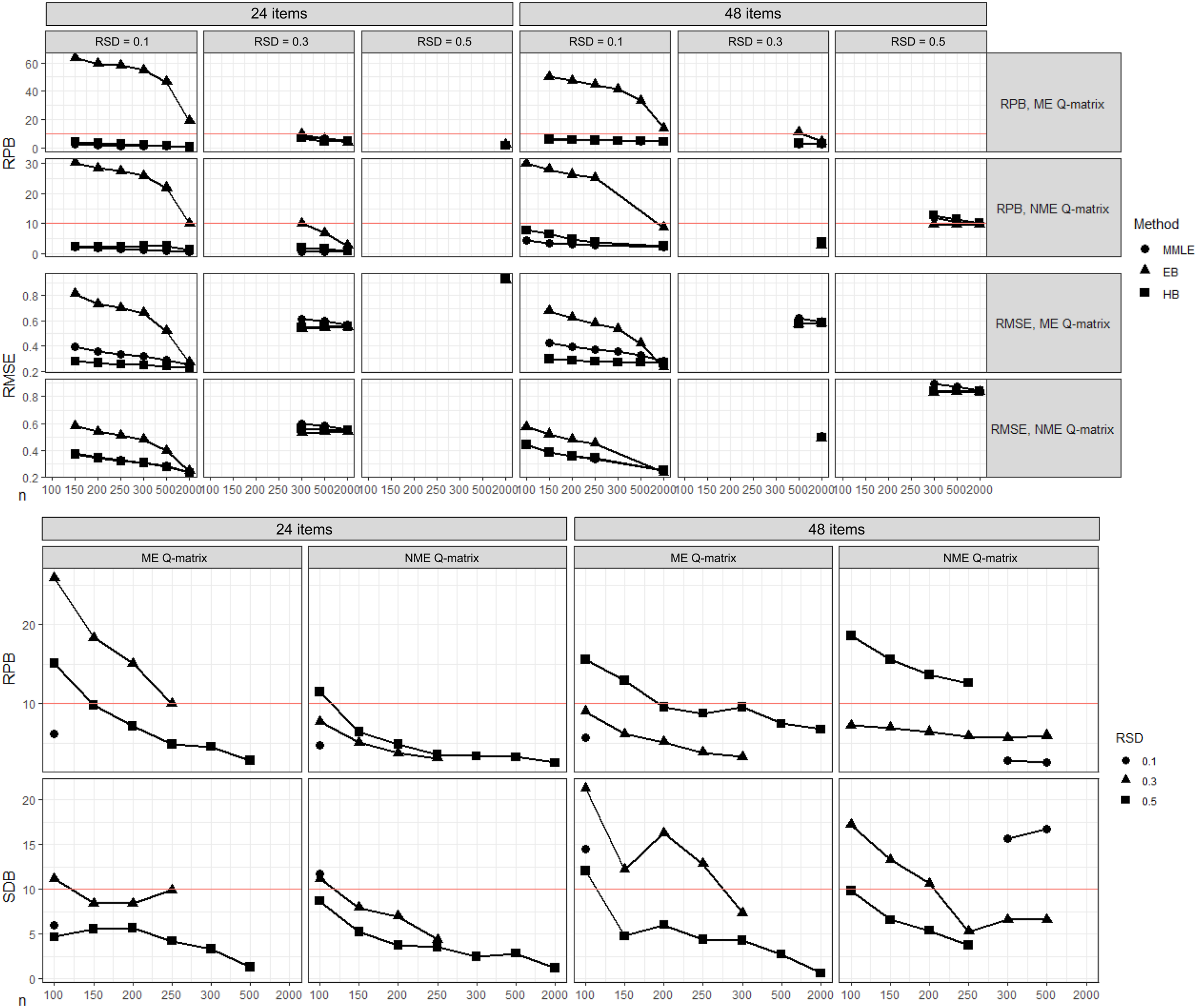

As shown in Figure 1 (top), of the 36 conditions that MMLE had 100% convergence, empirical Bayes had the lowest RPB of the three methods in 5 of those conditions (24 ME items and RSD = .3 with 2000 persons, 48 NME items and RSD = .3 with 2000 persons, and 48 NME item and RSD = .5 with 300, 500, and 2000 persons). Hierarchical Bayes had the lowest RPB in 10 conditions (24 ME items and RSD = .1 with 2000 persons, 24 ME items and RSD = .3 with 300 and 500 persons, 24 ME items and RSD = .5 with 2000 persons, and 48 ME items and RSD = .1 with all sample sizes $\geq 150$ persons). Although MMLE had the lowest RPB in the remaining 21 conditions, MMLE and hierarchical Bayes had highly comparable RPB (within 1.73%) in 34 of the 36 conditions (and within 3.56% for all conditions). Empirical Bayes had the highest RPB of the three methods in 30 of the 36 conditions, and even in the 5 conditions where empirical Bayes had the lowest RPB it still had comparable RPB to MMLE (within 2.16%). Empirical Bayes had unacceptably high RPB (RPB > 10%) in 24 conditions. Alternatively, MMLE and hierarchical Bayes had acceptably low RPB in 33 of the 36 conditions, with these methods only having unacceptably high RPB in 3 conditions (48 NME items and RSD = .5 with 300, 500, and 2000 persons). These results agree with our hypothesis regarding RPB that hierarchical Bayes $<$ empirical Bayes, but disagree with our hypothesis that empirical Bayes $<$ MMLE (as empirical Bayes consistently had the largest RPB of the three methods). This unexpected pattern was evident in conditions with RSD = .1, where MMLE obtained accurate item parameter estimates with 100% convergence in the presence of item parameters with small variability.

As shown in Figure 1 (top), of the 36 conditions that MMLE had 100% convergence, MMLE had the lowest RMSE in 3 conditions (48 NME items and RSD = .1 with 150, 200, and 250 persons), and empirical Bayes had the lowest RMSE of the three methods in 15 conditions (24 ME items and RSD = .3 with 300, 500, and 2000 persons, 24 ME items and RSD = .5 with 2000 persons, 48 ME items and RSD = .1 with 2000 persons, 48 ME items and RSD = .3 with 500 and 2000 persons, 24 NME items and RSD = .3 with 300, 500, and 2000 persons, 48 NME items and RSD = .1 with 2000 persons, 48 NME items and RSD = .3 with 2000 persons, and 48 NME items and RSD = .5 with 300, 500, and 2000 persons). Hierarchical Bayes had the lowest RMSE of the three methods in 19 conditions, generally having the lowest RMSE in the conditions with RSD = .1 (except for the condition with 48 ME items, RSD = .1, and 2000 persons, where empirical Bayes had the lowest RMSE).⁹ As seen in Figure 1 (top), hierarchical Bayes had lower or similar RMSE (at most .035 higher than the best method) in every condition. Although empirical Bayes had lower RMSE than hierarchical Bayes in more conditions, empirical Bayes had extremely high RMSE in several conditions (most notably those with RSD = .1). Based on these results, we concluded that hierarchical Bayes was the best of the three methods regarding RMSE, having lower or comparable RMSE to MMLE and empirical Bayes in all conditions. In general, MMLE outperformed empirical Bayes (having lower or comparable RMSE) in the conditions with RSD = .1, whereas empirical Bayes outperformed MMLE in the conditions with RSD $\geq 0.3$ . These results agree with our hypotheses regarding RMSE that hierarchical Bayes $<$ MMLE, and hierarchical Bayes $<$ empirical Bayes (as hierarchical Bayes consistently had the smallest or comparable RMSE of the three methods). However, these results only somewhat agree with our hypothesis that empirical Bayes $<$ MMLE, as empirical Bayes only had notably lower RMSE than MMLE in conditions where RSD $\geq 0.3$ . Figure 1 (top) illustrates that the accuracy of empirical Bayes was notably worse relative to MMLE and hierarchical Bayes for conditions with RSD = .1 and sample sizes less than 2000. However, the differences between the two methods diminish as RSD and/or sample size increase. To summarize the results for research question 1a, hierarchical Bayes outperformed both MMLE and empirical Bayes, having RPB generally comparable to MMLE and lower or comparable RMSE to both MMLE and empirical Bayes across the conditions analyzed.

Research Question 1b: Acceptability of Hierarchical Bayes

In the following analysis, we evaluate the acceptability of hierarchical Bayes with item covariates as an alternative to MMLE in the 48 conditions that MMLE failed to achieve 100% convergence. We examine the RPB and SDB of estimates obtained by hierarchical Bayes with item covariates in these conditions.¹⁰ Figure 1 (bottom) shows the RPB and SDB for hierarchical Bayes with covariates in the 48 conditions that MMLE failed to achieve 100% convergence.

As shown in Figure 1 (bottom), hierarchical Bayes with covariates had acceptable RPB $(< 10 %)$ in 37 of the 48 conditions, having unacceptable RPB in the other 11 conditions (24 ME items and RSD = .3 with 100, 150, and 200 persons, 24 ME items and RSD = .5 with 100 persons, 48 ME items and RSD = .5 with 100 and 150 persons, 24 NME items and RSD = .5 with 100 persons, and 48 NME items and RSD = .5 with all sample sizes $\leq 250$ persons). The primary factors affecting the acceptability of RPB in hierarchical Bayes with covariates was the number of persons and RSD (with hierarchical Bayes only having unacceptable RPB in conditions with sample sizes $\leq 250$ persons and RSD $\geq 0.3$ ). In addition, hierarchical Bayes with covariates had acceptable SDB $(< 10 %)$ in 34 of the 48 conditions, having unacceptable SDB in the other 14 conditions (24 ME items and RSD = .3 with 100 persons, 48 ME items and RSD = .1 with 100 persons, 48 ME items and RSD = .3 with all sample sizes $\leq 250$ persons, 48 ME items and RSD = .5 with 100 persons, 24 NME items and RSD = .1 with 100 persons, 24 NME items and RSD = .3 with 100 persons, 48 NME items and RSD = .1 with 500 persons, and 48 NME items and RSD = .3 with all sample sizes $\leq 200$ persons). Similar to RPB, the primary factors affecting SDB in hierarchical Bayes with covariates was the number of persons and RSD (with all but one of the conditions with unacceptable SDB having a sample size $\leq 300$ persons). However, in contrast with RPB (where conditions with larger RSD were more likely to have unacceptably high RPB), all but one of the conditions with unacceptably high SDB had smaller RSD $(\leq 0.3)$ , and all conditions with RSD = .5 had acceptable SDB.

Taking both RPB and SDB into consideration, hierarchical Bayes with item covariates was an acceptable alternative to MMLE (having both RPB < 10% and SDB < 10%) in 25 of the 48 conditions that MMLE failed to converge in 100% of replications. In general, hierarchical Bayes was more likely to be an acceptable alternative to MMLE in conditions with less (24) items, conditions with larger $(\geq 0.3)$ RSD, and conditions with larger $(\geq 250)$ sample sizes.

Research Question 2: Added Accuracy of Item Covariates

Figure 2 (top) presents the RPB and RMSE for hierarchical Bayes with covariates and hierarchical Bayes without covariates in all 42 ME Q-matrix conditions.¹¹ Each point in Figure 2 (top) represents the maximum RPB or maximum RMSE for all item parameter types, with each item parameter type averaged across replications.

Figure 2.

Simulation Results for Research Question 2 (top) and Research Question 3 (bottom). Note. Horizontal lines indicate cutoff for acceptable RPB and SDB (10%).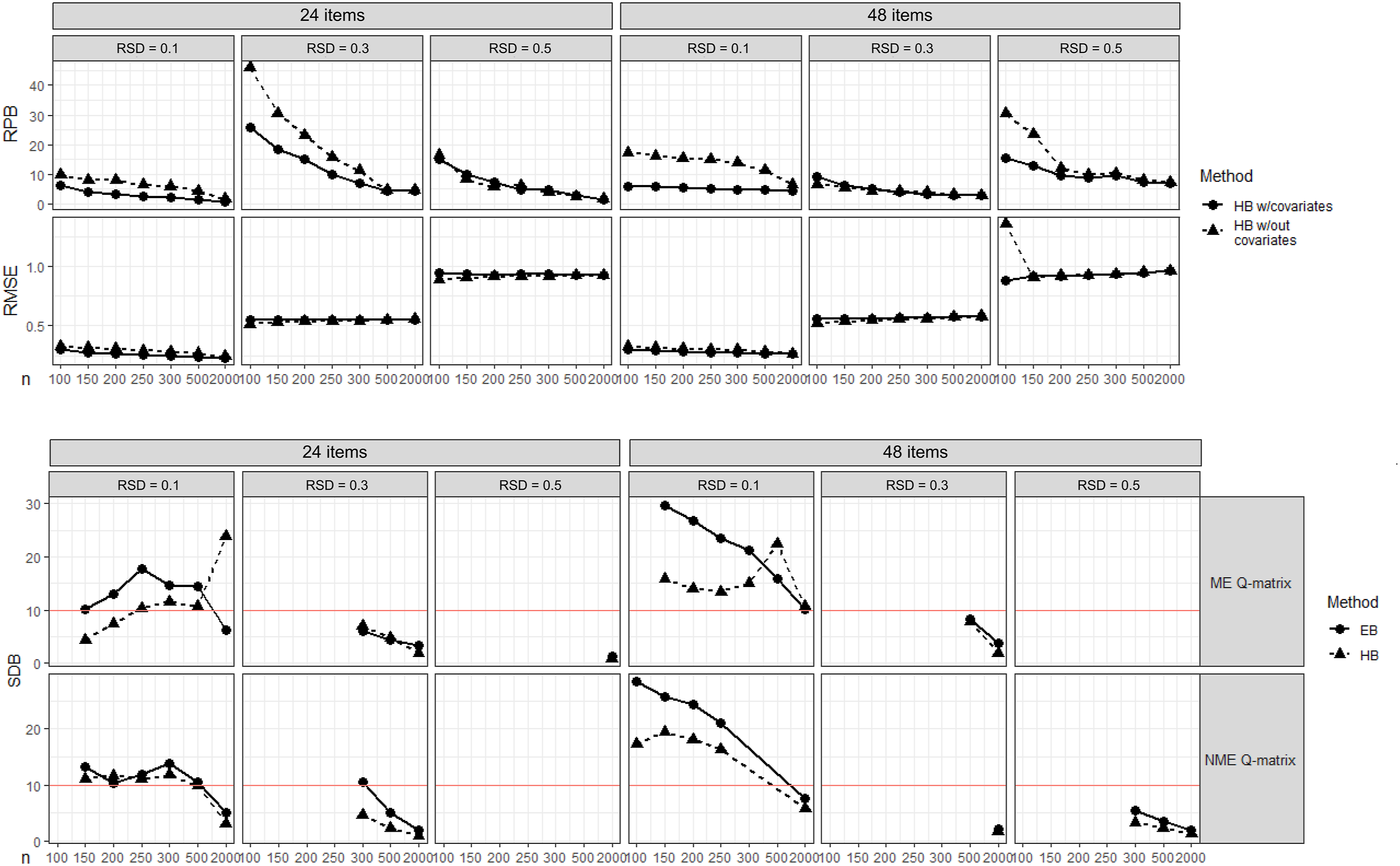

As shown in Figure 2 (top), hierarchical Bayes without covariates only had lower RPB than hierarchical Bayes with covariates in 9 of the 42 conditions (24 ME items and RSD = .3 with 500 and 2000 persons, 24 ME items and RSD = .5 with 150, 200, 300, and 500 persons, and 48 ME items and RSD = .3 with all sample sizes $\leq 200$ persons), whereas hierarchical Bayes with covariates had lower RPB in the other 33 conditions. Additionally, results were largely comparable (within 2.58%) between the two methods in the 9 conditions where hierarchical Bayes without covariates performed better than hierarchical Bayes with covariates. These results agree with our hypothesis regarding RPB that hierarchical Bayes with item covariates $<$ hierarchical Bayes without item covariates, as hierarchical Bayes with item covariates had lower (or comparable) RPB to hierarchical Bayes without item covariates in all conditions.

Hierarchical Bayes with covariates had unacceptable RPB (≥10%) in 6 of the 42 conditions (24 ME items and RSD = .3 with all sample sizes $\leq 200$ persons, 24 ME items and RSD = .5 with 100 persons, and 48 items and RSD = .5 with 100 and 150 persons), and hierarchical Bayes without covariates had unacceptable RPB in 16 of the 42 conditions (24 ME items and RSD = .3 with all sample sizes $\leq 300$ , 24 ME items and RSD = .5 with 100 persons, 48 ME items and RSD = .1 with all sample sizes $\leq 500$ , and 48 ME items and RSD = .5 with all sample sizes $\leq 300$ ). There were no conditions where hierarchical Bayes without covariates had acceptable RPB and hierarchical Bayes with item covariates had unacceptable RPB. These results agree with our hypothesis that, regarding RPB, hierarchical Bayes with item covariates $<$ hierarchical Bayes without item covariates.

As shown in Figure 2 (top), hierarchical Bayes with covariates had lower RMSE than hierarchical Bayes without item covariates in 16 of the 42 conditions. Although hierarchical Bayes without covariates had lower RMSE in the remaining 26 conditions, results were highly comparable between the two methods, with differences in RMSE $< 0.06$ for all but one condition. In one condition (48 ME items and RSD = .5 with 100 persons), hierarchical Bayes without item covariates had significantly higher RMSE (1.364) than either method in any other condition. The most significant factor affecting RMSE for both methods was RSD, with both methods having larger RMSE as RSD increased. To summarize the results for research question 2, hierarchical Bayes with covariates typically outperformed hierarchical Bayes without covariates, having lower (or comparable) RPB and lower (or comparable) RMSE in all 42 conditions.

Research Question 3: Accuracy of Posterior SD Estimates

Figure 2 (bottom) presents the SDB for empirical Bayes and hierarchical Bayes with item covariates in the 36 conditions that MMLE had 100% convergence. Each point in Figure 2 (bottom) represents the maximum SDB for all item parameter types, with each item parameter type averaged across replications.

As shown in Figure 2 (bottom), of the 36 conditions that MMLE had 100% convergence, empirical Bayes had lower SDB than hierarchical Bayes with covariates in 5 conditions (24 ME items and RSD = .3 with 2000 persons, 48 NME items and RSD = .3 with 2000 persons, and 48 NME items and RSD = .5 with 300, 500, and 2000 persons). However, hierarchical Bayes had similar SDB (within 3.07%) to empirical Bayes in these conditions. Hierarchical Bayes with covariates had lower SDB than empirical Bayes in the remaining 31 conditions, having SDB as much as 59.5% lower than empirical Bayes in these conditions. A few noteworthy exceptions to these results were observed in the condition with 24 ME items and RSD = .1 with 2000 people (Figure 2 [bottom], top-left) and the condition with 48 ME items and RSD = .1 with 500 persons (Figure 2 [bottom], fourth column, top), which both had sudden increases in SDB for hierarchical Bayes relative to similar conditions with different sample sizes. These sudden increases resulted from scaling artifacts of SDB occurring when the MCSE in the denominator was close to 0, despite posterior SD estimates and MCSE both decreasing with an increasing number of persons.¹²

As presented in Figure 2 (bottom), empirical Bayes had unacceptably high SDB (SDB > 10%) in 24 conditions (including all but one of the conditions with RSD = .1). Hierarchical Bayes had unacceptably high SDB in 3 conditions (48 NME items and RSD = .5 with 300, 500, and 2000 persons), and acceptably low SDB in the remaining 33 conditions. These results agree with our hypothesis that, in general, regarding SDB, hierarchical Bayes $<$ empirical Bayes. To summarize the results for research question 3, hierarchical Bayes with item covariates typically had lower SDB than empirical Bayes in the conditions that MMLE had 100% convergence.

Results Regarding Simulation Factors

With respect to the four simulation factors, results were largely consistent with our hypotheses (presented in Appendix D) regarding RPB and SDB with a few exceptions: RPB decreased with increasing the number of persons, the number of items, and RSD, and with NME Q-matrices; and SDB decreased with increasing the number of persons and decreasing the number of items. RMSE was less effected by changes in the simulation factors than expected, either changing as expected (e.g., increasing for MMLE with an increase in the number of items) or exhibiting minimal change. This is likely because, as observed in the simulation results, the simulation factor with the greatest impact on RMSE is RSD (with RMSE increasing as RSD increases for all methods), with other simulation factors only having a minimal effect on RMSE.

Summary and Discussion

MMLE is commonly used for estimating item parameters within an IRT framework. However, MMLE’s accuracy, as well as its ability to achieve convergence, is limited in small sample sizes. Mislevy (1988) showed that auxiliary item information can be used to increase the accuracy of Rasch item location estimates with an empirical Bayes method. We presented hierarchical Bayes as an alternative to empirical Bayes both because RSD can be underestimated by empirical Bayes due to ignoring the uncertainty of item parameter estimates and because empirical Bayes is unable to obtain item parameter estimates when MMLE fails to achieve convergence. In this paper, we showed how item covariates can be used in empirical Bayes and hierarchical Bayes to obtain item parameter estimates of a GRM with higher accuracy and precision in small to medium sample sizes.

Method Selection Guideline

We provide a general guideline in Figure F1 in Appendix F based on simulation results regarding which method is recommended for different conditions. Step 1. The first step is to determine whether or not there are usable item covariates available and whether the test is unidimensional or multidimensional. If there are no item covariates available, then empirical Bayes and hierarchical Bayes with item covariates are not viable options. Step 2a. If there are no usable item covariates and/or the test is multidimensional, then stop considering the proposed method. Step 2b. If there are usable item covariates and the test is unidimensional, we make the following recommendations based on the Q-matrix structure, the number of items, and the RSD of those items. Step 3. To determine which method is recommended (given the availability of item covariates and the number of items), estimates of the RSD are required. These estimates do not need to be highly accurate, but rather capable of allowing RSD to be categorizable as small (e.g., RSD = .1), medium (e.g., RSD = .3), or large (e.g., RSD = .5). To obtain such estimates of the RSD, classical item discriminations and thresholds can be obtained to calculate linear regression RSD estimates. We provide an R function to calculate the linear regression RSD estimates based on classical item discriminations and thresholds on GitHub (https://github.com/naveirmd/Auxiliary_Item_Information_GRM). Step 3a. If there are a smaller number of items (e.g., 24), we make the following recommendations based on the RSD of items. If there is a small RSD (e.g., RSD = .1, indicating items within groups are highly similar), for an ME Q-matrix, we recommend using hierarchical Bayes with item covariates for sample sizes between 100 and 200 and MMLE for sample sizes $\geq 250$ , and for an NME Q-matrix, we recommend using MMLE for sample sizes between 150 and 300 and hierarchical Bayes for sample sizes $\geq 500$ . If there is a medium RSD (e.g., RSD = .3, indicating that items within groups are similar yet distinctly different), we recommend hierarchical Bayes with item covariates for sample sizes $\geq 250$ with an ME Q-matrix or $\geq 150$ with an NME Q-matrix. If there is a large RSD (e.g., RSD = .5, indicating that items within groups are highly dissimilar), we recommend hierarchical Bayes with item covariates for sample sizes $\geq 150$ with either an ME or NME Q-matrix. Step 3b. If there is a larger number of items (e.g., 48), we make the following recommendations based on the RSD of items. If there is a small RSD (e.g., RSD = .1), for an ME Q-matrix, we recommend MMLE for sample sizes $\geq 150$ , and for an NME Q-matrix, we recommend MMLE for sample sizes $\geq 100$ and hierarchical Bayes for sample sizes $\geq 2000$ . If there is a medium RSD (e.g., RSD = .3), we recommend hierarchical Bayes with item covariates for sample sizes $\geq 300$ with an ME Q-matrix, or $\geq 250$ with an NME Q-matrix. If there is a large RSD (e.g., RSD = .5), for an ME Q-matrix, we recommend hierarchical Bayes with item covariates for sample sizes $\geq 200$ , and for an NME Q-matrix, we recommend empirical Bayes for sample sizes $\geq 300$ .

Item Covariate Specification

As shown in this study, hierarchical Bayes with item covariates can be an acceptable alternative to MMLE under certain conditions. However, the effectiveness of hierarchical Bayes is dependent on the correct specification of the item covariates structure. Both exploratory factor analysis and observation of the salient features of items are useful for assigning items to their correct groups and for assuring the item covariate structure is correct. Exploratory factor analysis can be used to identify how many dimensions (or domains within a single dimension) there are, and factor loadings can identify which items likely belong to each dimension/domain. The salient features of items (such as their similarities to other items with similar covariate structures) can be used to interpret these factors/dimensions in meaningful ways to make the classification of future items easier. Mislevy (1988) illustrated how imposing a linear model on Rasch item location parameters based on item groupings can highlight misclassified items. Items with distinctly different properties than other items in their groups, such as an item with a significantly higher difficulty than any other item in its group, may indicate an incorrect item covariate structure. Looking at such items’ salient features may show if (and how) they were misclassified, and what method of correcting the item covariate structure should be used. In Mislevy’s (1988) empirical example, he shows three different methods that can be implemented to correct a misidentified item covariate structure: removing misfit items, creating a new item group, and changing the group status of certain items. Similar approaches can be applied to identifying and correcting errors in the item covariate structure of a GRM.

Study Limitations

This study had several methodological limitations that can be addressed in future research on these topics. First, only two item covariate structures (mutually exclusive binary Q-matrices and non-mutually-exclusive Q-matrices, both with 6 item covariates and constant covariate effects across simulation conditions) were used in this simulation study to reflect the predominant covariate structures observed from an extensive literature review. In this study, we also make the assumption that items are unidimensional, with item groups representing domains within a single underlying dimension. Future research using different item covariate structures, different effects of item covariates, and generalizing these methods to allow multidimensionality may yield interesting results.

Second, in this study, we assumed that the item covariate structure was correctly specified. The purpose of this study was to evaluate the added value of a correctly identified item covariate structure through the use of empirical Bayes and hierarchical Bayes methods. The preliminary process of specifying the item covariate structure correctly is outside the scope of this study. Mislevy (1986) addressed how mispecifying the item covariate structure can result in “ensemble biases” affecting entire groups of items. Such biases can cause statistical properties (such as consistency) to no longer apply to item parameter estimates. Future research regarding the full repercussions of using an incorrect item covariate structure on empirical Bayes and hierarchical Bayes methods could be of interest.

Third, the levels selected for simulation factors (number of persons, number of items, and magnitude of RSD) reflect those we considered most relevant based on the literature. However, using additional levels of these simulation factors (e.g., 36 items, RSD = .7) could show more clearly how evaluation criteria (RPB, RMSE, and SDB) change as a function of these simulation factors, such as comparing SDB for conditions with 24, 36, and 48 items.

Fourth, in this study, we extended Mislevy’s (1988) empirical Bayes method for a Rasch model to a GRM. One advantage of Mislevy’s (1988) three-step approach is that the full item response data is not needed when MMLE is documented beforehand. However, the use of a three-step empirical Bayes method made it impossible to obtain results when MMLE was unable to converge. Because of this limitation, empirical Bayes and hierarchical Bayes could not be compared in the 48 simulation conditions of which MMLE was unable to achieve convergence in 100% of replications. Empirical Bayes, as it is most commonly used in the literature, is a one-step procedure similar in implementation to hierarchical Bayes, but with different prior and posterior distribution specifications. However, a hierarchical Bayes method would allow hyperparameters to be estimated from hyper-prior distributions (e.g., the second line of Equation (8)), an empirical Bayes method would treat these hyperparameters as fixed. Both a one-step empirical Bayes method and a one-step hierarchical Bayes method could be implemented using MCMC (in software such as rStan), allowing results to be obtainable when MMLE is unable to achieve convergence. A one-step empirical Bayes method could be used in future research to allow empirical Bayes to be compared with hierarchical Bayes methods.

Fifth, this study focused on the use of weakly informative priors on means and standard deviations for a hierarchical Bayes method with auxiliary item information. It is expected that the use of informative priors on parameters leads to accurate and stable estimates when the prior distributions are matched with the “true” distributions of the parameters in a one-step empirical Bayes method (e.g., Natesan et al. [2016] for binary item response models) or in a marginalized Bayes modal (MAP; Mislevy, 1986; Tsutakawa & Lin, 1986) method without auxiliary item information. For the purpose of comparing MAP to the hierarchical Bayes approach with auxiliary item information, MAP with informative priors on item parameters (α_i ∼ logN (0, .5²); β_i1 ∼ N (−2, 1); β_i2 ∼ N (−1, 1); β_i3 ∼ N (1, 1); β_i4 ∼ N (2, 1), which are matched with the “true” distributions in the current study) was used to estimate item parameters in the conditions where MMLE estimates were not obtained. As in MMLE, MAP estimates of item parameters could not be obtained when item categories had zero responses due to extreme thresholds that were caused by large RSD or small sample sizes. However, additional simulation studies are required to evaluate the relative performance of weakly informative priors in a hierarchical Bayes method with auxiliary item information, with comparisons between multiple hypothesized “true” distributions driven from empirical studies in a one-step empirical Bayes method with and without auxiliary item information and in MAP (without auxiliary item information).

Conclusions

In this paper, we have demonstrated the viability of a hierarchical Bayes method as alternatives to MMLE in small sample sizes. In addition, we have shown how to implement these methods using item covariates, and in what conditions these methods can result in acceptably accurate estimates of item parameters and RSD. Despite the aforementioned limitations of this study, we have demonstrated these methods and their implementation in conditions reflecting those most commonly found in the literature, and we have presented a framework that can be used in future research to expand upon these results under various other research conditions. In addition, we have provided the R functions written and utilized in this study to obtain empirical Bayes and hierarchical Bayes estimates for researchers to implement these proposed methods to their own research.

Supplemental Material

Supplemental Material - Using Auxiliary Item Information in the Item Parameter Estimation of a Graded Response Model for a Small to Medium Sample Size: Empirical Versus Hierarchical Bayes Estimation

Supplemental Material for Using Auxiliary Item Information in the Item Parameter Estimation of a Graded Response Model for a Small to Medium Sample Size: Empirical Versus Hierarchical Bayes Estimation by Matthew Naveiras and Sun-Joo Cho in Applied Psychological Measurement

Footnotes

Acknowledgments

We would like to express our sincere gratitude to the Editor, Associate Editor, and the reviewers for their invaluable and constructive feedback on this paper.

Declaration of Conflicting Interests

The author(s) declared no potential conflicts of interest with respect to the research, authorship, and/or publication of this article.

Funding

The author(s) received no financial support for the research, authorship, and/or publication of this article.

ORCID iD

Matthew Naveiras

Supplemental Material

Supplemental material for this article is available online.

Notes

References

Baker

F. B.

(1993). Sensitivity of the linear logistic test model to misspecification of the weight matrix. Applied Psychological Measurement, 17(3), 201–210. https://doi.org/10.1177/014662169301700301

Baker

F. B.

Kim

S.-H.

(2004). Item response theory: Parameter estimation techniques (2nd ed.). Dekker.

Bock

R. D.

Aitkin

(1981). Marginal maximum likelihood estimation of item parameters: Application of an EM algorithm. Psychometrika, 46(4), 443–459. http://dx.doi.org/10.1007/BF02293801

Chalmers

R. P.

(2012). mirt: A multidimensional item response theory package for the R environment. Journal of Statistical Software, 48(6), 1–29. http://doi:10.18637/jss.v048.i06

Cho

S.-J.

De Boeck

Embretson

Rabe-Hesketh

(2013). Additive multilevel item structure models with random residuals: Item modeling for explanation and item generation. Psychometrika, 79(1), 84–104. http://doi.org/10.1007/s11336-013-9360-2

Cho

S.-J.

De Boeck

Lee

(2017). Evaluating testing, profile likelihood confidence interval estimation, and model comparisons for item covariate effects in linear logistic test models. Applied Psychological Measurement, 41(5), 353–371. http://doi.org/10.1177/0146621617692078.

Curtis

(2010). BUGS code for item response theory. Journal of Statistical Software, 36 (Code Snippet 1), 1–34. http://dx.doi.org/10.18637/jss.v036.c01

De Boeck

(2008). Random item IRT models. Psychometrika, 73(4), 533–559. https://doi.org/10.1007/s11336-008-9092-x

De Boeck

Wilson

(2004). Explanatory item response models: A generalized linear and nonlinear approach. Springer.

10.

Fischer

H. F.

Rose

(2019). Scoring depression on a common metric: A comparison of EAP estimation, plausible value imputation, and full Bayesian IRT modeling. Multivariate Behavioral Research, 54(1), 85–99. https://doi.org/10.1080/00273171.2018.1491381

11.

Forero

C. G.

Maydeu-Olivares

(2009). Estimation of IRT graded response models: Limited versus full information methods. Psychological Methods, 14(3), 275–299. http://doi.org/10.1037/a0015825

12.

Fox

J. P.

(2010). Bayesian item response modeling: Theory and applications. Springer New York. https://doi.org/10.1007/978-1-4419-0742-4

13.

Gelman

(2006). Prior distributions for variance parameters in hierarchical models (comment on article by Browne and Draper). Bayesian Analysis, 1(3), 515–534. http://doi.org/10.1214/06-BA117A

14.

Gelman

Carlin

J. B.

Stern

H. S.

Rubin

D. B.

(2014). Bayesian data analysis (vol. 2). Chapman and Hall.

15.

Kieftenbeld

Natesan

(2012). Recovery of graded response model parameters: A comparison of marginal maximum likelihood and Markov chain Monte Carlo estimation. Applied Psychological Measurement, 36(5), 399–419. https://doi.org/10.1177/0146621612446170

16.

Koehler

Brown

Haneuse

S. J.

(2009). On the assessment of Monte Carlo error in simulation-based statistical analyses. The American Statistician, 63(2), 155–162. https://doi:10.1198/tast.2009.0030

17.

Mislevy

R. J.

(1986). Bayes modal estimation in item response models. Psychometrika, 51(2), 177–195. https://doi.org/10.1007/BF02293979

18.

Mislevy

R. J.

(1988). Exploiting auxiliary information about items in the estimation of Rasch item difficulty parameters. Applied Psychological Measurement, 12(3), 281–296. https://doi.org/10.1177/014662168801200306

19.

Natesan

Nandakumar

Minka

Rubright

J. D.

(2016). Bayesian prior choice in IRT estimation using MCMC and variational Bayes. Frontiers in Psychology, 7, 1422. https://doi.org/10.3389/fpsyg.2016.01422.

20.

R Core Team . (2018). R: A language and environment for statistical computing. R Foundation for Statistical Computing. Retrieved from. http://www.R-project.org/

21.

Reise

S. P.

(1990). Parameter recovery in the graded response model using MULTILOG. Journal of Educational Measurement, 27(2), 133–144. https://doi.org/10.1111/j.1745-3984.1990.tb00738.x

22.

Rencher

A. C.

(2000). Linear models in statistics. Wiley.

23.

Samejima

(1969). Estimation of latent ability using a response pattern of graded scores. Psychometrika, 34(S1), 1–97. http://doi.org/10.1007/BF03372160

24.

Stan Development Team . (2018). rStan: the R interface to Stan. R package version 2.17.3. Retrieved from https://cran.r-project.org/web/packages/rstan/citation.html

25.

Tsutakawa

R. K.

Lin

H. Y.

(1986). Bayesian estimation of item response curves. Psychometrika, 51(2), 251–267. https://doi.org/10.1007/bf02293983

Supplementary Material

Please find the following supplemental material available below.

For Open Access articles published under a Creative Commons License, all supplemental material carries the same license as the article it is associated with.

For non-Open Access articles published, all supplemental material carries a non-exclusive license, and permission requests for re-use of supplemental material or any part of supplemental material shall be sent directly to the copyright owner as specified in the copyright notice associated with the article.

0.00 MB

0.65 MB