Sage Journals: Discover world-class research

Abstract

When developing ordinal rating scales, we may include potentially unordered response options such as “Neither Agree nor Disagree,” “Neutral,” “Don’t Know,” “No Opinion,” or “Hard to Say.” To handle responses to a mixture of ordered and unordered options, Huggins-Manley et al. (2018) proposed a class of semi-ordered models under the unidimensional item response theory framework. This study extends the concept of semi-ordered models into the area of diagnostic classification models. Specifically, we propose a flexible framework of semi-ordered DCMs that accommodates most earlier DCMs and allows for analyzing the relationship between those potentially unordered responses and the measured traits. Results from an operational study and two simulation studies show that the proposed framework can incorporate both ordered and non-ordered responses into the estimation of the latent traits and thus provide useful information about both the items and the respondents.

Keywords

diagnostic classification model rating scales nominal response option ordinal response option neutral responses semi-ordered model

Classification of respondents with a set of characteristics or competencies is often of interest in social and behavioral sciences research. These characteristics are frequently measured using rating scales where respondents are scored on their selections from ordinal options such as “Strongly Disagree,” “Disagree,” “Agree,” and “Strongly Agree.” On those types of scales, it is common to offer a “no opinion” option such as “Neither Agree nor Disagree,” “Neutral,” “Don’t Know,” “No Opinion,” or “Hard to Say” (Schuman & Presser, 1996). For example, a rating scale measuring the perception of drug risk used by the United Nations Drug Control Program offers the following five response options: “No Risk,” “Slight Risk,” “Moderate Risk,” “Great Risk,” and “Don’t Know” for questions such as “What do you think the level of risk is for a person who has taken tranquilizers at some time?” (Bejarano et al., 2011). The “no-opinion” options may be potentially non-ordered with the original ordinal scale and pose questions about how to best handle them.

Traditional psychometric approaches could treat item responses as either ordinal or nominal, but not a mixture of both. Huggins-Manley et al. (2018) proposed a class of semi-ordered item response theory (IRT) models which could handle a mixture of ordinal and nominal item responses. Using the semi-ordered IRT models, Huggins-Manley et al. (2018) treated the selection of a “Not Applicable” response option as a selection of a nominal variable on an otherwise ordinal scale. Later, Cohn and Huggins-Manley (2020) applied the semi-ordered models where the “Neutral” responses were treated as nominal variables on an ordinal scale, and Zhou and Huggins-Manley (2020) applied the semi-ordered models where item-level missingness was treated as an intentional selection of a nominal variable on an ordinal scale. The semi-ordered models allow for (1) analyzing responses on both ordered and unordered options at the same time, and (2) examining the relationship between the unordered option and the measured trait in the IRT framework.

Outside of the IRT framework, diagnostic classification models (DCMs; Rupp et al., 2010), a newer class of psychometric models, have demonstrated their potential to accurately classify examinees according to their latent traits. For example, Templin and Henson (2006) used DCMs to classify patients with pathological gambling disorder, Liu and Shi (2020) used DCMs to classify individuals with different personalities, and Ahn and Feuerstahler (2021) used DCMs to classify employees with organizational commitment. Compared to expert-suggested approaches for classifications, DCMs offered a new set of methods for researchers and practitioners to obtain data-suggested classifications. The purpose of this study is to extend the semi-ordered concept into the world of DCMs by proposing and evaluating a semi-ordered DCM framework that can analyze responses on a mix of ordered and unordered options. In the next section, we introduce the foundational work that supports the development of the semi-ordered DCMs.

Foundational Work

The proposed semi-order DCM framework extends three strands of psychometric work: (1) the integration of the nominal response model (NRM; Bock, 1972) and ordinal IRT models in Huggins-Manley et al. (2018); (2) the nominal response diagnostic model (NRDM) developed in Templin et al. (2008) to handle nominal data; (3) the ordinal response diagnostic model (ORDM) developed in Liu and Jiang (2018) to handle ordinal data.

The Semi-ordered IRT Models

When nominal response options are present in an ordinal scale, traditional measurement models are unable to handle such scenarios. Huggins-Manley et al. (2018) presented an example where a questionnaire asks about respondents’ family support. One item on the questionnaire asks whether the respondent “Never,” “Seldom,” “Sometimes,” “Usually,” or “Always” has time to be with spouse/partner. On this ordinal scale, an additional nominal response option: “Not Applicable” is provided for those that do not have partners. As a result, the scale is a mix of ordinal and nominal options. Similarly, Cohn and Huggins-Manley (2020) presented another example where the “Neutral” option is considered nominal within an ordinal scale.

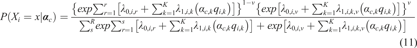
To address situations like above, Huggins-Manley et al. (2018) proposed a class of semi-ordered IRT models, most notably the semi-ordered generalized partial credit model (semi-GPCM), in which the nominal and ordinal responses are calibrated at the same time. The semi-GPCM integrates the NRM and the GPCM (Muraki, 1992) innovatively. If all the options are nominal (e.g., selecting your favorite color from blue, red, orange, gold, and green), an NRM could be used, which defines the probability of selecting response option r on item i given a unidimensional latent trait $θ$ for examinee j as

P (X_{i} = r | θ_{j}) = \frac{\exp (d_{i r} θ_{j} + b_{i r})}{\sum_{r = 1}^{R} \exp (d_{i r} θ_{j} + b_{i r})}

(1)

where

d_{i r}

and

b_{i r}

are the slope parameter and intercept parameter for option r on item i, respectively. Equation (1) models the likelihood of selecting option

r

as compared to the sum of the likelihood of selecting each response option. Thus, the NRM can be considered a manifestation of the “divide-by-total” approach in polytomous item response modeling (Thissen & Steinberg, 1986).

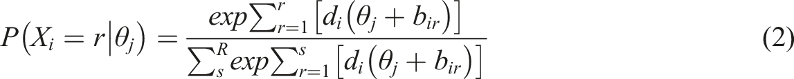
Comparatively, when all response options are ordinal, one could use the GPCM, which defines the probability of selecting response option r on item i given a unidimensional latent trait $θ$ for examinee j as

P (X_{i} = r | θ_{j}) = \frac{\exp \sum_{r = 1}^{r} [d_{i} (θ_{j} + b_{i r})]}{\sum_{s}^{R} \exp \sum_{r = 1}^{s} [d_{i} (θ_{j} + b_{i r})]}

(2)

Comparing the NRM with the GPCM, the NRM slope parameter $d_{i r}$ becomes $r \times d_{i}$ in the GPCM for each response option r, signifying that the GPCM treats responses as ordinal variables. Despite that, the GPCM shares a similar structure with the NRM because both models use the “divide-by-total” approach and the GPCM can be seen as a special case of the NRM. Such a relationship made the integration of the two models possible in Huggins-Manley et al. (2018). Let v denote the unordered response option, which can be, for example, “Neutral,” or “Don’t Know” options. The semi-GPCM defines the probability of selecting the unordered option $v$ on item i given a unidimensional latent trait $θ$ for examinee j as

P (X_{i} = v | θ_{j}) = \frac{\exp (d_{i v} θ_{j} + b_{i v})}{\sum_{s}^{R} \exp \sum_{r = 1}^{s} [d_{i} (θ_{j} + b_{i r})] + \exp (d_{i v} θ_{j} + b_{i v})}

(3)

We can see that the semi-GPCM utilizes the basic structure of the NRM while allowing the ordered response options to be analyzed through the GPCM component. This type of semi-ordered model allows us to examine the relationship between a latent variable and responses on both ordered and unordered options. Now, let us move on to the world of DCMs, particularly the models that are able to handle unordered and ordered responses, respectively.

The NRDM

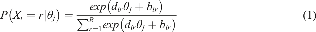
DCMs are confirmatory latent class models with different parameterizations of the measurement component and/or the structural component. The latent classes are formulated through the possession and non-possession states of multiple categorical latent traits. In this article, we use $k = 1, \dots, K$ to index binary latent traits (aka attributes) and $α_{c} = {α_{1}, \dots, α_{K}}$ to index attribute profiles for latent class c. To specify the relationship between items and attributes, we construct an item-by-attribute incidence matrix, commonly referred to as a Q-matrix (Tatsuoka, 1983). In a Q-matrix, an entry $q_{i k} = 1$ when item i measures attribute k, and $q_{i k} = 0$ otherwise.

Among all DCMs, the NRDM in Templin et al. (2008) was developed to handle nominal responses. The NRDM defines the probability of examinees in latent class c selecting response option r on item i, such that

P (X_{i} = r | α_{c}) = \frac{\exp [λ_{0, i, r} + λ_{i, r}^{T} h (α_{c}, q_{i})]}{\sum_{r = 1}^{R} \exp [λ_{0, i, r} + λ_{i, r}^{T} h (α_{c}, q_{i})]}

(4)

where

λ_{0, i, r}

is the intercept associated with option r on item i, and

λ_{i, r}^{T} h (α_{c}, q_{i})

index all the main effects and higher-order interaction effects of the k attributes associated with option r on item i, which can be expressedas

\sum_{k = 1}^{K} λ_{1, i, k, r} (α_{c, k} q_{i, k}) + \sum_{k = 1}^{K - 1} \sum_{k^{'} = k + 1}^{K} λ_{2, i, k, k^{'}, r} (α_{c, k} α_{c, k^{'}} q_{i, k} q_{i, k^{'}}) + \dots + λ_{K, i, 1, \dots, K, r} \prod_{k = 1}^{K} (α_{c, k} q_{i, k})

The ORDM

To create semi-ordered DCMs, ordinal DCMs that utilize the “divide-by-total” approach similar to the NRDM are needed. Among all polytomous DCMs, the ORDM is one possible candidate.

The ORDM defines the probability of examinees in latent class c selecting response option r on item i, such that

P (X_{i} = r | α_{c}) = \frac{\exp \sum_{r = 1}^{r} [λ_{0, i, r} + λ_{i}^{T} h (α_{c}, q_{i})]}{\sum_{s}^{R} \exp \sum_{r = 1}^{s} [λ_{0, i, r} + λ_{i}^{T} h (α_{c}, q_{i})]}

(5)

Comparing the NRDM with the ORDM, the NRDM $λ_{i, r}$ vector becomes $r \times λ_{i}$ in the ORDM for each response option r, representing the ordinal nature of response options. Despite that, the ORDM is similarly structured with the NRDM using the “divide-by-total” approach and the ORDM can be seen as a special case of the NRDM. The relationship between the NRDM and the ORDM is similar to that between the NRM and the GPCM, which creates an opportunity for developing a semi-ordered DCM.

The Semi-ordered DCM Framework

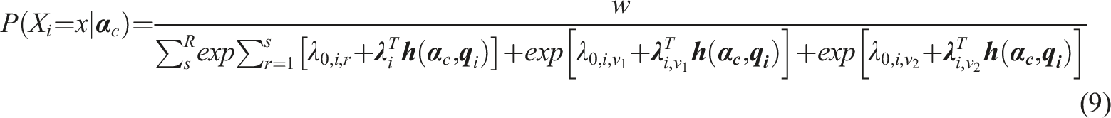
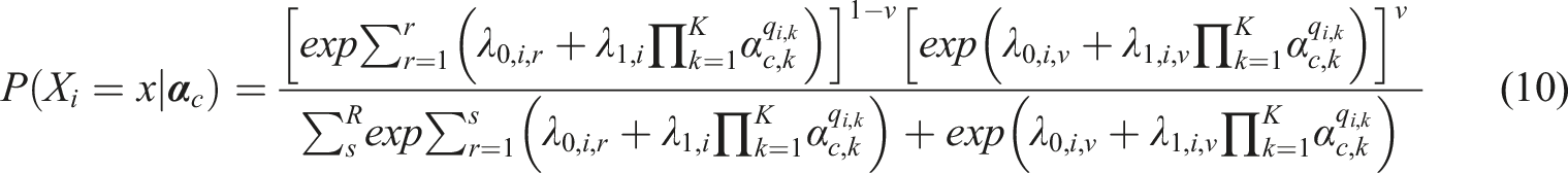
The semi-ordered DCM (SDCM) framework integrates the NRDM and the ORDM similar to the approach used in Huggins-Manley et al. (2018). Depending on whether an examinee selects an ordinal response option r or a nominal response option v, the SDCM can be written as

P (X_{i} = x | α_{c}) = \frac{{\exp \sum_{r = 1}^{r} [λ_{0, i, r} + λ_{i}^{T} h (α_{c}, q_{i})]}^{1 - v} {\exp [λ_{0, i, v} + λ_{i, v}^{T} h (α_{c}, q_{i})]}^{v}}{\sum_{s}^{R} \exp \sum_{r = 1}^{s} [λ_{0, i, r} + λ_{i}^{T} h (α_{c}, q_{i})] + \exp [λ_{0, i, v} + λ_{i, v}^{T} h (α_{c}, q_{i})]}

(6)

where v is a binary indicator representing whether an examinee selects the nominal response option (v=1) or not (v=0). The SDCM in equation (6) can be broken down into two levels: it defines the probability of examinees in latent class c selecting an ordered response option r on item i as

P (X_{i} = r | α_{c}) = \frac{\exp \sum_{r = 1}^{r} [λ_{0, i, r} + λ_{i}^{T} h (α_{c}, q_{i})]}{\sum_{s}^{R} \exp \sum_{r = 1}^{s} [λ_{0, i, r} + λ_{i}^{T} h (α_{c}, q_{i})] + \exp [λ_{0, i, v} + λ_{i, v}^{T} h (α_{c}, q_{i})]}

(7)

and selecting the nominal option v such as “Neither Agree nor Disagree,” “Neutral,” “Don’t Know,” “No Opinion,” or “Hard to Say” as

P (X_{i} = v | α_{c}) = \frac{\exp [λ_{0, i, v} + λ_{i, v}^{T} h (α_{c}, q_{i})]}{\sum_{s}^{R} \exp \sum_{r = 1}^{s} [λ_{0, i, r} + λ_{i}^{T} h (α_{c}, q_{i})] + \exp [λ_{0, i, v} + λ_{i, v}^{T} h (α_{c}, q_{i})]}

(8)

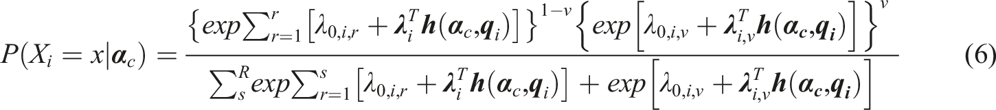
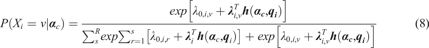
Equations (7) and (8) share the same denominator while differing only on the numerator. Note that the parameters for the main effect and interaction effect on the ordered response options do not have subscript r, instead, they are functioning as $r \times λ_{i}$ , similar to the ORDM.

If multiple nominal response options are present in an ordinal scale, for example: both “Neutral” $(v_{1})$ and “Don’t Know” $(v_{2})$ are added in a Likert scale, we can expand the SDCM to accommodate multiple nominal response options such that

P (X_{i} = x | α_{c}) = \frac{w}{\sum_{s}^{R} \exp \sum_{r = 1}^{s} [λ_{0, i, r} + λ_{i}^{T} h (α_{c}, q_{i})] + \exp [λ_{0, i, v_{1}} + λ_{i, v_{1}}^{T} h (α_{c}, q_{i})] + \exp [λ_{0, i, v_{2}} + λ_{i, v_{2}}^{T} h (α_{c}, q_{i})]}

(9)

where

w = \exp \sum_{r = 1}^{r} [λ_{0, i, r} + λ_{i}^{T} h (α_{c}, q_{i})]

when an ordered response option r is selected,

w = \exp [λ_{0, i, v_{1}} + λ_{i, v_{1}}^{T} h (α_{c}, q_{i})]

when “Neutral”

(v_{1})

is selected, and

w = \exp [λ_{0, i, v_{2}} + λ_{i, v_{2}}^{T} h (α_{c}, q_{i})]

when “Don’t Know”

(v_{2})

is selected.

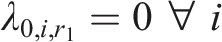
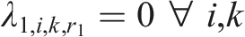
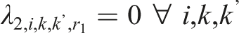
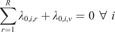
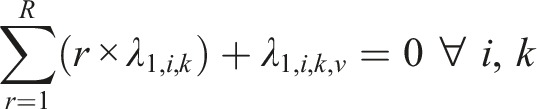
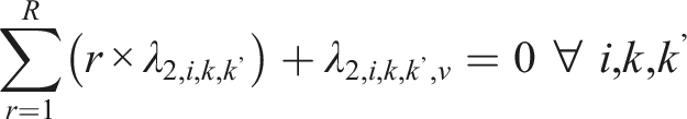
Two types of constraints are imposed on the SDCM, one for identifiability, and the other one for reasonable interpretations of parameter estimates. For identifiability, one could adopt either one of the following two types of constraints. First, the “first-as-zero” approach (Thissen, 1991) can be used where the parameters associated with the first response option are fixed to zero, such that

λ_{0, i, r_{1}} = 0 \forall i

λ_{1, i, k, r_{1}} = 0 \forall i, k

λ_{2, i, k, k^{'}, r_{1}} = 0 \forall i, k, k^{'}

and for all higher-order interactions. Alternatively, the “sum-to-zero” approach used in Bock (1972) and Templin et al. (2008) can be used where the sum of each type of parameter (i.e., intercepts, main effects, and interaction effects) is fixed to 0, such that

\sum_{r = 1}^{R} λ_{0, i, r} + λ_{0, i, v} = 0 \forall i

\sum_{r = 1}^{R} (r \times λ_{1, i, k}) + λ_{1, i, k, v} = 0 \forall i, k

\sum_{r = 1}^{R} (r \times λ_{2, i, k, k^{'}}) + λ_{2, i, k, k^{'}, v} = 0 \forall i, k, k^{'}

and for all higher-order interactions. For reasonable interpretations of parameter estimates, the main effect and interaction effect parameters for the ordered response options are constrained to be greater than 0. This constraint ensures that possessing an attribute does not decrease the probability of selecting a higher response option on the ordinal scale. This constraint is similar to fixing the discrimination parameter to be greater than 0 under an IRT model so that examinees that are higher on the latent trait continuum are likely to endorse a higher response option. Such constraint is not imposed on the main effects associated with the unordered response option (i.e.,

λ_{1, i, k, v}

) because possessing an attribute may or may not increase the probability of selecting the unordered response option.

In operational settings, the total number of parameters associated with the SDCM will be somewhere between that of the ORDM and the NRDM for a given dataset. Let us illustrate the SDCM in detail using a hypothetical example. Suppose there are 20 items on a five-point scale: “Strongly Disagree,” “Disagree,” “Neutral”, “Agree,” and “Strongly Agree” where 10 items measure $α_{1}$ and the other 10 items measure $α_{2}$ with no cross-loadings. Traditionally, one could fit an ORDM to this dataset because of the ordinal nature of the response options. Under the ORDM, we would need to estimate a total of 120 parameters: 20 items $\times$ 5 options = 100 intercepts $(λ_{0, i, r})$ and 20 main effects $(λ_{1, i})$ . If we ignore the ordinal nature and treat the item responses as nominal variables, one could fit an NRDM with 200 parameters: 20 items $\times$ 5 options = 100 intercepts $(λ_{0, i, r})$ and 20 items $\times$ 5 options = 100 main effects $(λ_{1, i, r})$ . If one wants to evaluate whether the “Neutral” option conforms to the order within the five-point scale, an SDCM could be implemented with 140 parameters: 20 items $\times$ 5 options = 100 intercepts $(λ_{0, i, r})$ , 20 main effects for the ordered responses $(λ_{1, i})$ , and 20 main effects for the “Neutral” option $(λ_{1, i, v})$ . Note that the SDCM can accommodate unordered response options, but the response options do not have to be unordered if one wants to implement the SDCM. Modeling the “Neutral” option as unordered is an example. If the “Neutral” option is actually ordered, the SDCM will produce similar results to the ORDM. If the “Neutral” option is found to be unordered, the SDCM can uncover the true relationship between that option and the attributes. In short, the SDCM provides the flexibility of incorporating such a relationship which may or may not be present in a dataset.

Like any general model with interaction parameters, the number of parameters is always a concern in data collection and estimation. If there were cross-loadings with more attributes in the above example, the number of parameters in the general SDCM could easily be close to or exceed 1000. One potential solution for this issue is to develop smaller models that are nested within the SDCM which feature a smaller number of parameters. The SDCM provides a flexible framework that could accommodate most earlier DCMs to serve as its core item response function (IRF). For example, the earliest and simplest DCM: “deterministic inputs, noisy, and gate” (DINA) model (Haertel, 1989; Junker & Sijtsma, 2001) can be converted into an SDCM-DINA. In the SDCM-DINA, each item has four sets of parameters: an intercept $(λ_{0, i, r})$ for each ordered response option, an overall attribute(s) effect $(λ_{1, i})$ for the ordered response options, an intercept $(λ_{0, i, v})$ for the unordered response option, and an overall attribute(s) effect $(λ_{1, i, v})$ for the unordered response option. The SDCM-DINA can be expressed as

P (X_{i} = x | α_{c}) = \frac{{[\exp \sum_{r = 1}^{r} (λ_{0, i, r} + λ_{1, i} \prod_{k = 1}^{K} α_{c, k}^{q_{i, k}})]}^{1 - v} {[\exp (λ_{0, i, v} + λ_{1, i, v} \prod_{k = 1}^{K} α_{c, k}^{q_{i, k}})]}^{v}}{\sum_{s}^{R} \exp \sum_{r = 1}^{s} (λ_{0, i, r} + λ_{1, i} \prod_{k = 1}^{K} α_{c, k}^{q_{i, k}}) + \exp (λ_{0, i, v} + λ_{1, i, v} \prod_{k = 1}^{K} α_{c, k}^{q_{i, k}})}

(10)

Using the SDCM-DINA, the number of parameters is immune from the number of attributes and/or cross-loadings, which may be more favorable in some operational settings.

In addition to the SDCM-DINA, we could also develop another nested model using the IRF of the linear logistic model (LLM; Maris, 1999). The SDCM-LLM can be viewed as the general SDCM without all the interactions. It can be written as

P (X_{i} = x | α_{c}) = \frac{{\exp \sum_{r = 1}^{r} [λ_{0, i, r} + \sum_{k = 1}^{K} λ_{1, i, k} (α_{c, k} q_{i, k})]}^{1 - v} {\exp [λ_{0, i, v} + \sum_{k = 1}^{K} λ_{1, i, k, v} (α_{c, k} q_{i, k})]}^{v}}{\sum_{s}^{R} \exp \sum_{r = 1}^{s} [λ_{0, i, r} + \sum_{k = 1}^{K} λ_{1, i, k} (α_{c, k} q_{i, k})] + \exp [λ_{0, i, v} + \sum_{k = 1}^{K} λ_{1, i, k, v} (α_{c, k} q_{i, k})]}

(11)

Using the SDCM-LLM, the number of parameters is still being affected by the number of attributes but not by the number of cross-loadings. There are other earlier DCMs that can be used as IRFs under the SDCM framework, and the selection of a particular IRF involves careful considerations of both construct theories and statistical properties.

Operational Study

In operational settings, whether the “Neither Agree nor Disagree” or “Neutral” options are ordered or unordered is often unknown. This section aims to demonstrate how to use the SDCM to accommodate that unknown situation through an operational dataset. Both the SDCM and the ORDM were fit to the dataset in which the results were compared.

Method

We obtained 901 examinees’ responses to 40 items on a part of an experiment DISC personality test in the International Personality Item Pool (Goldberg et al., 2006) with no missing data. Those 40 items are all simple-structured items where each item only measures one attribute. Items 1-10 measure assertiveness $(α_{1})$ , items 11-20 measure social confidence $(α_{2})$ , items 21-30 measure adventurousness $(α_{3})$ , and item 31-40 measure dominance $(α_{4})$ . Personality attributes sometimes are hypothesized as categorical variables for the use of user marketing on social media websites such as Facebook (e.g., Souri et al., 2018), or personnel administration in a workspace (e.g., Coe, 1992). Users of personality tests may also be interested in their personality categories, for example, whether they can be classified as an extrovert or an introvert. DCMs provide an alternative model-based classification avenue to the traditional standard-setting approach based on experts’ opinions (Rupp et al., 2010; Templin & Henson, 2006). In our dataset, we hypothesized attributes as categorical variables (e.g., being adventurous vs. not adventurous) to demonstrate the use of DCMs.

Each item in the dataset has five response options: “Strongly Disagree,” “Disagree,” “Neutral,” “Agree,” and “Strongly Agree.” Before the analysis, negatively worded items were reverse coded back to make sure that the direction of response options aligned with that of the latent trait continuum. For example, both item 2 and item 7 measure assertiveness $(α_{1})$ , while item 2 is positively worded: “I try to lead others,” and item 7 is negatively worded: “I wait for others to lead the way.” Before computing any descriptive statistics, we first reverse-coded the responses on item 7. This reverse-coding step is necessary because most psychometric models, including the SDCM and the ORDM, employ the dominance-based process philosophy (Coombs, 1964), which assumes that the probability of agreeing with a statement monotonically increases as individuals’ latent trait level increases on the continuum.

Figure S1 in the Online Appendix visualizes the distribution of examinees’ response option selections across all items. We can see that most examinees selected “Agree” or “Strongly Agree” on most items. As a result, we would expect that the estimated probability of selecting those two options would be higher than the other three options from the fitted models. Under the SDCM, the four unneutral options were treated as ordinal variables and the “Neutral” option was treated as a nominal variable. Under the ORDM, all five options were treated as ordinal variables.

This dataset was chosen for the operational study because selecting the “Neutral” option may or may not be directly related to the measured attributes. For example, selecting “Neutral” on an item measuring assertiveness $(α_{1})$ may or may not be a reflection of a lack of possessing assertiveness $(α_{1})$ . Through fitting both the ORDM and the SDCM, we would be able to look at whether the non-ordered treatment of the “Neutral” option would change the probability of selecting the “Neutral” option on each item.

Parameters for both models were estimated using Hamiltonian Monte Carlo (HMC; Duane et al., 1987) algorithms in Stan (Carpenter et al., 2017). The full Stan code is shared in the Online Appendix. For each response option on each item, the prior distribution was specified as $Normal (0,2)$ for the intercept and $Normal (1.5, 2)$ for the main effects. Four chains were run for each model where each chain took 10,000 iterations with the first 5000 discarded as burn-in. The Gelman-Rubin convergence statistic $\hat{R}$ (Brooks & Gelman, 1998; Gelman & Rubin, 1992) was used to assess convergence. All the $\hat{R}$ values for each parameter in both models were very close to 1.00, suggesting convergence to a stationary distribution (Junker et al., 2016).

To assess absolute fit, posterior predictive p-values (PPPs; Gelman et al., 2013) were computed for each item model where values close to 0.5 suggest good fit. Specifically, we simulated 20,000 new datasets based on the 20,000 draws from the posterior distribution. Then we computed the root mean square error of approximation (RMSEA, Kunina-Habenicht et al., 2009) based on the difference between the estimated and expected number of individuals in each attribute profile. The PPPs were then computed as the percentage of the simulated data whose RMSEA was greater than or equal that of the real data.

To compare the relative fit between the models, the leave-one-out information criterion (LOOIC; Vehtari et al., 2017) values were computed using the importance-sampling algorithm (Gelfand et al., 1992), where smaller values suggest better fit.

Results

Model Fit

The average PPPs across items for the SDCM and the ORDM were 0.53 and 0.54, respectively, both indicating good fit. The LOOIC values for the SDCM and the ORDM were 77.1 and 78.5, respectively, suggesting that the SDCM fit slightly better than the ORDM. It is worth mentioning that this does not mean that the SDCM will be universally better fitting than the ORDM. It is just the SDCM may fit slightly better than the ORDM on this dataset, suggesting that the “Neutral” option may be unordered overall across items. If one uses another dataset where the “Neutral” may be ordered within the ordinal scale, they may find that the ORDM fits better than the SDCM. For the absolute fit indices such as the PPPs, the more general SDCM may not always show better fit because it may not be as close to the data structure as the nested model. For relative fit indices such as the LOOIC, we found that it is more likely that the more general model fit better even when the nested model would be true. However, the choice of different priors may complicate the results and it remains unclear how the prior information for the additional parameters in the more general model may affect the values of relative fit indices.

Item Parameters

The mean and standard deviation of the posterior distribution for each item parameter were listed in the Online Appendix (Tables S1–S4) for the two models. According to model structures, the SDCM had six parameters associated with each item, while the ORDM had five. Under both models, the intercept and main effects for the first response option “Strongly Disagree” were fixed to zero. What is different is that the main effect for the “Neutral” option was estimated separately through using the $λ_{1, i, v}$ parameter in the SDCM, while the main effect parameter $λ_{1, i}$ was consistently applied to all response options in the ORDM. In terms of the accuracy of parameter estimation, we could compare the average standard deviation (similar to the use of standard error under the frequentist’s approach) of each type of parameter across all items. Such information can be found on the last row of Table S2 for the SDCM and Table S4 for the ORDM. The SDCM produced smaller average standard deviations than the ORDM on parameters that both models have. The SDCM had large standard deviations on the main effect parameter for the “Neutral” option. Such large standard errors of the parameters associated with the response option that was separately estimated were also observed when the semi-ordered models were used under the IRT framework (e.g., Cohn & Huggins-Manley, 2020; Huggins-Manley et al., 2018).

Although both the SDCM and the ORDM employ the divide-by-total approach to define category advancement similar to the GPCM under the IRT framework, the interpretation of parameter estimates under the SDCM and the ORDM is different from that under the GPCM. Under the GPCM, the $d_{i}$ is the slope (visually represented by the steepness of the item characteristic curve), and $b_{i r}$ is the point at which a person has an equal chance of scoring an $r - 1$ or $r$ . Under any DCM, because the latent traits are categorical instead of continuous, we won’t be able to have an item characteristic curve that is plotted along the latent trait continuum. Instead, we only have two values for each category in each item under a simple structure: the intercept $λ_{0, i, r}$ and the main effect $λ_{1, i}$ . A larger $λ_{0, i, r}$ is associated with a higher probability of endorsing option $r$ for persons that don’t possess the associated attributes, and a larger $λ_{1, i}$ is associated with a higher probability of endorsing option $r$ for persons that possess the associated attributes. We could conceptualize the overall difficulty of each response option in each item as $\sum_{r = 1}^{r} λ_{0, i, r} + r \times λ_{1, i}$ . We could also conceptualize the discrimination of each response option in each item as the difference in the probability of endorsing response option $r$ for people that possess and don’t possess the associate attributes. In other words, a higher discrimination is associated with a smaller $λ_{0, i, r}$ and a larger $λ_{1, i}$ . We can visualize this difference in probability more clearly in Figures 1–4, which are going to be presented in the next section.

Figure 1.

Example option characteristic curves in the operational study (Items 2 and 7 measuring assertiveness: $α_{1}$ ).

Figure 2.

Example option characteristic curves in the operational study (Items 12 and 16 measuring social confidence: $α_{2}$ ).

Figure 3.

Example option characteristic curves in the operational study (Items 24 and 27 measuring adventurousness: $α_{3}$ ).

Figure 4.

Example option characteristic curves in the operational study (Items 34 and 40 measuring dominance: 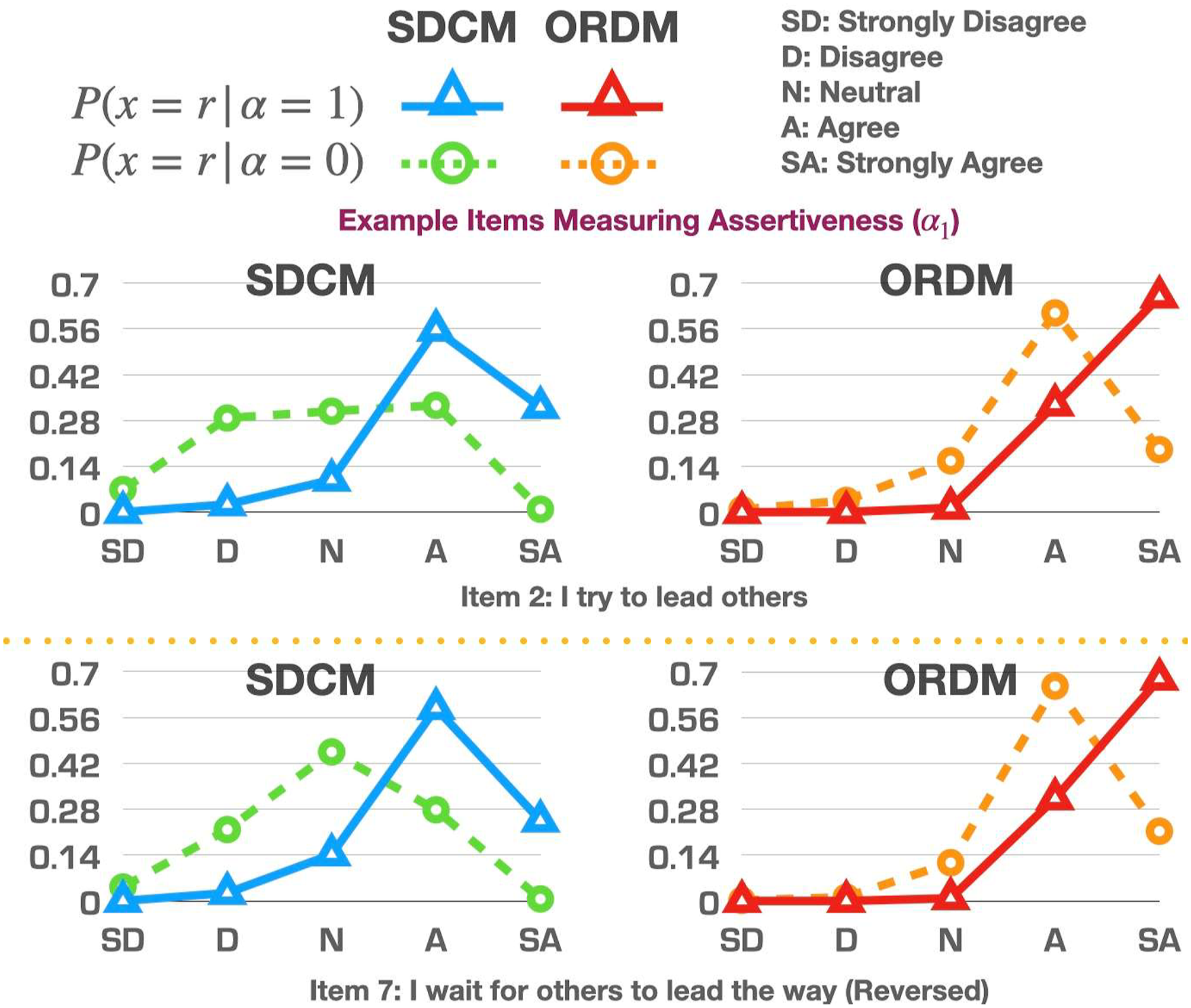$α_{4}$ ).

Rather than directly comparing the parameter estimates between the two models, it is more appropriate to compare when the parameter estimates are transformed back into probability because the denominators of the item models under the SDCM and the ORDM are different.

Category Response Probabilities

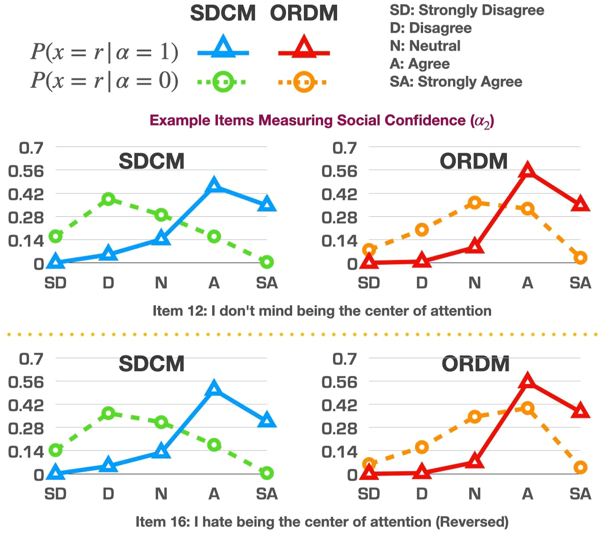
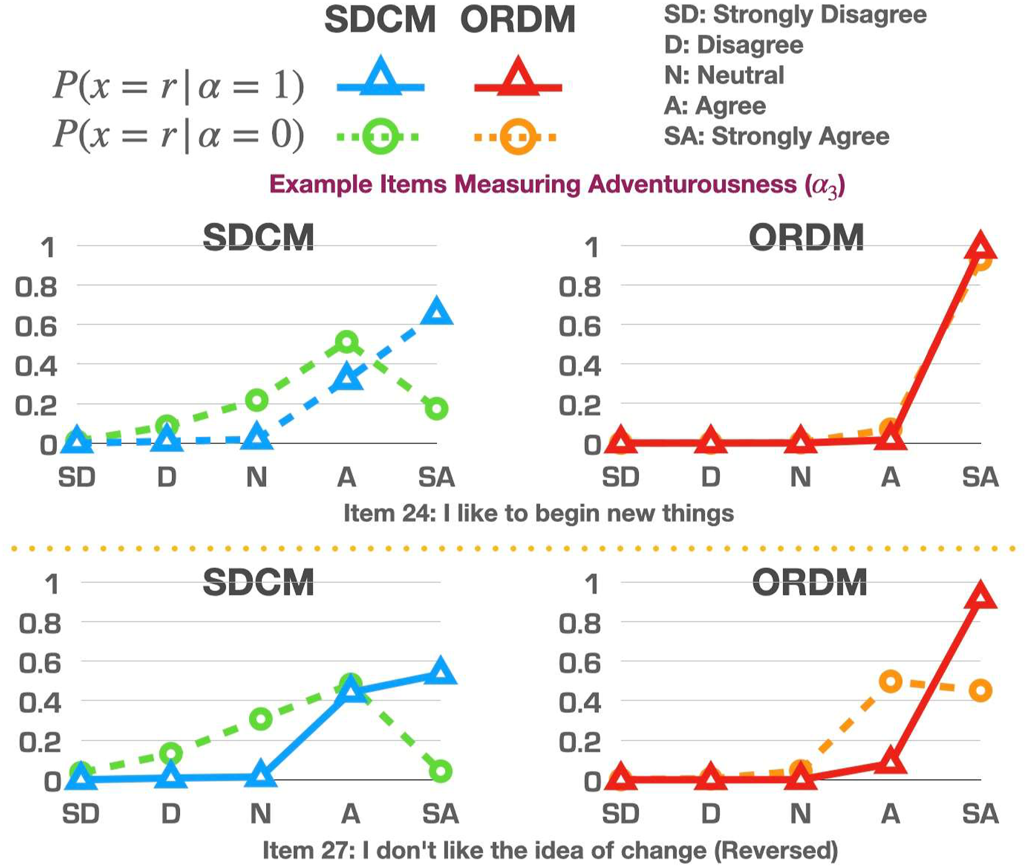
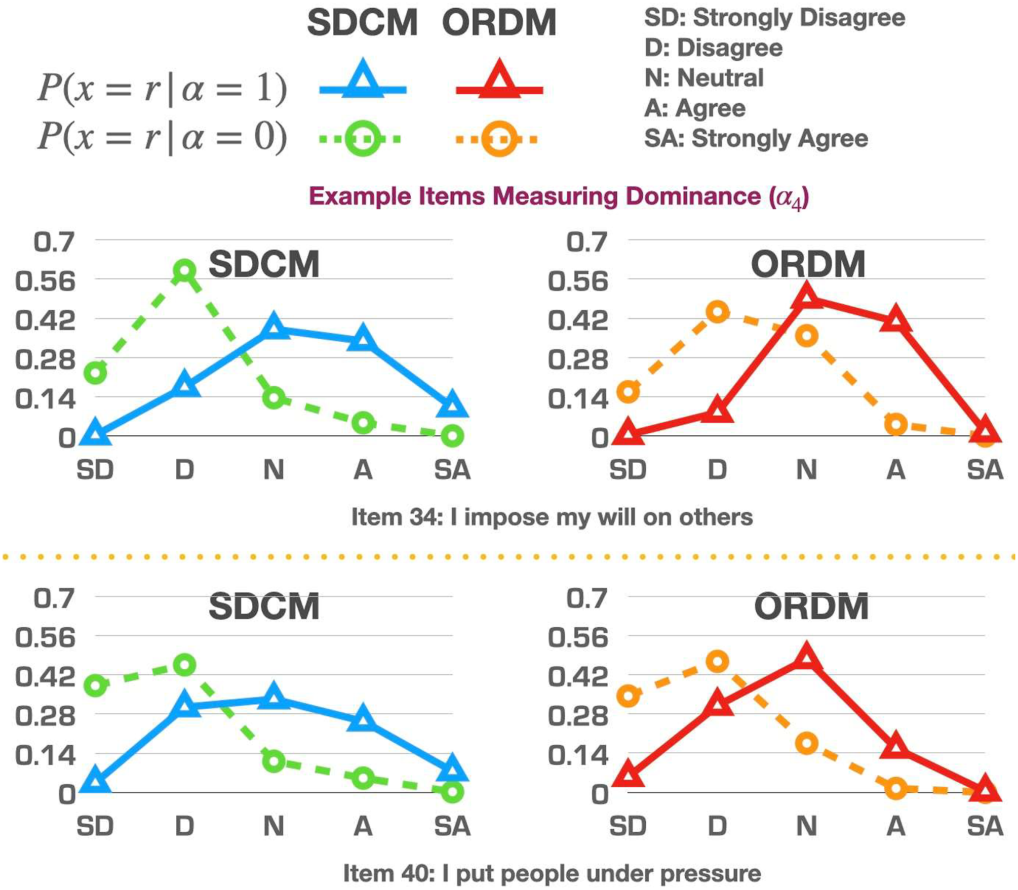
An easier way to examine the differences of the item parameter estimates between the two models is to input the parameter estimates into the models and compute the probabilities of selecting each response option on each item given the possession status of an attribute. Let us plot eight representative items (two for each attribute) in Figures 1–4 as examples for further discussion. Although those examples could be used for item revision and/or construct theory development, the focus here is to offer readers examples of how to read the graphs and understand the similarities/differences between the model estimates.

When comparing the curves produced by the SDCM and the ORDM, we could focus on their estimated probabilities of selecting “Neutral.” If those probabilities were similar to each other, it may suggest that the “Neutral” option may be ordered within its original scale. Although the two models’ different treatments on the “Neutral” option unavoidably affected the estimation of parameters of other response options, the focus of the comparison is on the “Neutral” option because that is the underlying reason for all the different estimates on other options.

In Figure 1, items 2 and 7 are examples where the “Neutral” option may be unordered because the probabilities of selecting the “Neutral” category between the two models are very different for either those who possess $α_{1}$ or not. The curves in item 2 are very similar to those in item 7 because the item stems are basically the same after reverse coding. As discussed previously, we expected that the probability of selecting “Agree” and “Strongly Agree” would be higher than other categories because more examinees selected those response options. That is why we can see that under the ORDM, those who did not possess assertiveness $(α_{1} = 0)$ had the highest probability of selecting “Agree,” and those who possessed assertiveness $(α_{1} = 1)$ had the highest probability of selecting “Strongly Agree.”

In contrast to items 2 and 7, the “Neutral” option may potentially be ordered within its original scale for items 12 and 16, as shown in Figure 2. The probabilities of selecting the “Neutral” option under the SDCM and the ORDM were very similar, suggesting that freely estimating the “Neutral” option in an unordered way may be similar to just constraining that option through an ordered fashion.

In Figure 3, items 24 and 27 were selected to illustrate the impact of the distribution of examinees selecting each response option. Recall from Figure S1 in the online appendix, most examinees selected “Agree” or “Strongly Agree.” As a result, the estimated probabilities of selecting the other three response options were expected to be lower. We observed that the SDCM was less confined to the original data distribution, as it gave a relatively smaller probability to the most frequently selected options compared to the ORDM.

In contrast to items 24 and 27, the original distributions of the data on items 34 and 40 were more balanced across different options. The category response probabilities estimated under the ORDM consistently followed the original distribution, and the SDCM produced similar estimates under this situation with more balanced data across response categories, as shown in Figure 4.

Lastly, we want to mention that each item under the SDCM or ORDM had its own model, and one could fit different models to different items based on a variety of factors such as absolute and relative item fit indices and the principle of parsimony. Model fitting is always an iterative process that connects to item development and revision.

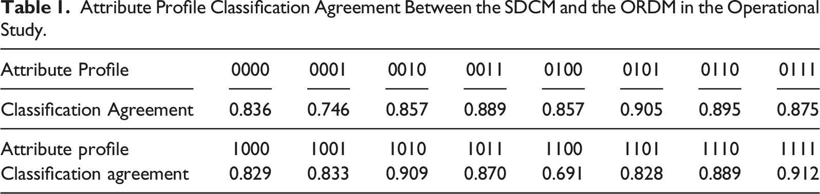
Classification Agreement

Ultimately, we are interested in examinees’ estimated scores under the two models. Examinees’ attribute classifications are their scores under the DCM framework. Table 1 provides the classification agreement on each attribute profile. Overall, 84.57% of examinees were classified with the same attribute profiles under the two models. In future applications of the SDCM, one may experience a higher or a lower agreement rate depending on how much the “Neutral” option deviates from the ordinal scale.

Table 1.

Attribute Profile Classification Agreement Between the SDCM and the ORDM in the Operational Study.

Attribute Profile	0000	0001	0010	0011	0100	0101	0110	0111
Classification Agreement	0.836	0.746	0.857	0.889	0.857	0.905	0.895	0.875
Attribute profile	1000	1001	1010	1011	1100	1101	1110	1111
Classification agreement	0.829	0.833	0.909	0.870	0.691	0.828	0.889	0.912

Simulation Study

Application of the SDCM to different items in the operational study demonstrated its utility in accommodating potentially unordered response options. In this section, we conducted two simulation studies to further explore the parameter estimation and classification accuracy between the SDCM and the ORDM. Both studies are couched within the conditions of the operational study, similar to Huggins-Manley et al. (2018) and Liu and Jiang (2018). We did not vary conditions such as sample size, number of attributes, test length, or Q-matrix complexity similar to the reasons identified in the aforementioned studies. The SDCM, as a special case of the NRDM, as well as an extension of the ORDM, obeys the general features that have been consistently uncovered through many DCM studies. For example, a larger sample size is associated with more accurate parameter estimation and a longer test length would increase classification accuracy, and a Q-matrix with more “1”s (i.e., more cross-loadings) may lead to lower classification accuracy (e.g., Madison & Bradshaw, 2015).

Study 1: SDCM is the True Model

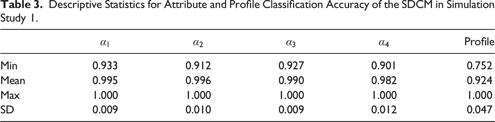
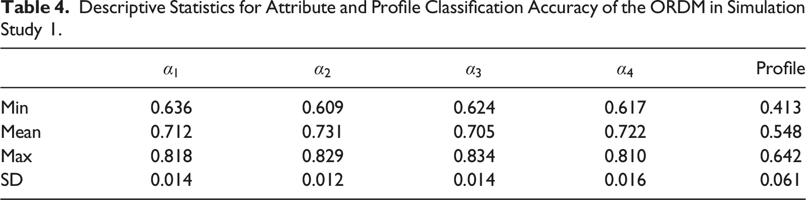
The purpose of Study 1 is two-fold. We aim to examine (1) whether the SDCM can produce unbiased parameter estimates, and classify individuals correctly, and (2) whether the performance of the SDCM is better than the ORDM when the data may be potentially unordered.

We generated 100 datasets using R (R Core Team, 2019) through the following four steps. First, we generated 901 persons’ true attribute profiles from a multinomial distribution of the profile proportions in the simulation study. Next, we extracted the true item parameters using the mean of the posterior distributions of each item parameter listed in Table S1. Then, the item and person parameters were submitted to the SDCM to compute the probability of selecting each response option on each item for each person. Finally, we drew a random number from the multinomial distribution of the response option probabilities for each item and person to serve as the person’s item response.

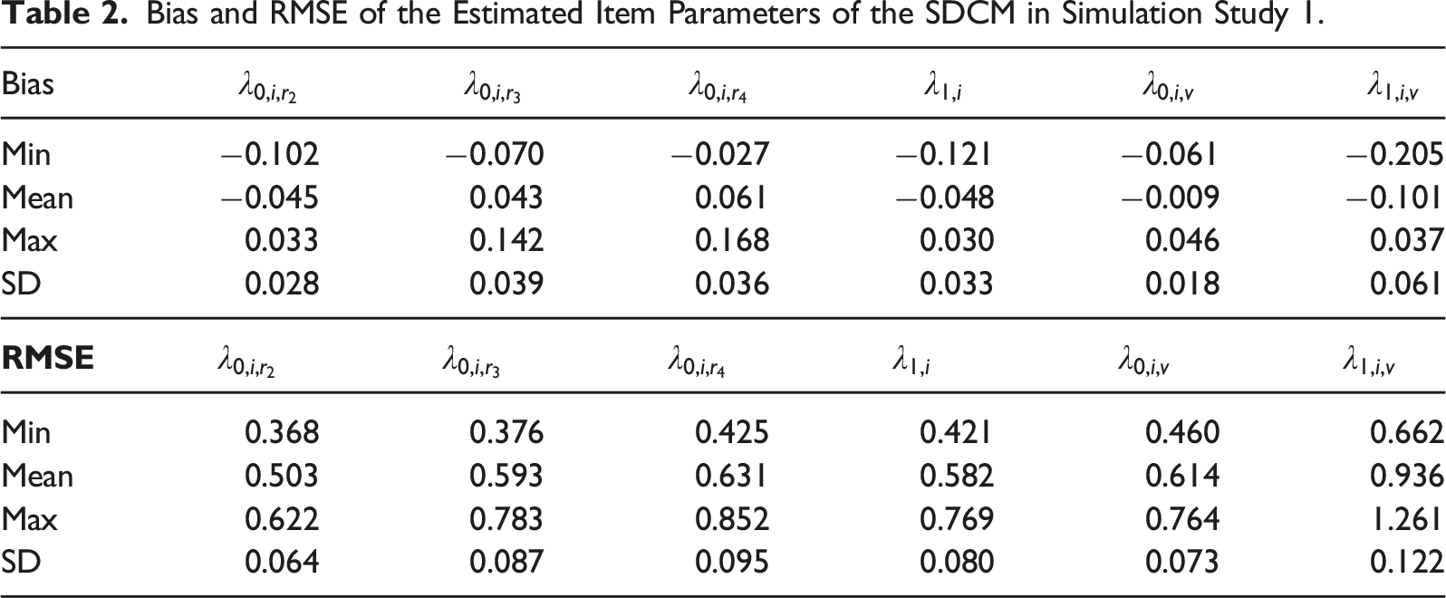
We then fit both the SDCM and the ORDM to each dataset using the same Stan code and HMC specifications for the operational study. To assess parameter recovery of the SDCM, we computed the bias and the root mean square error (RMSE) such that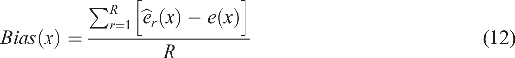

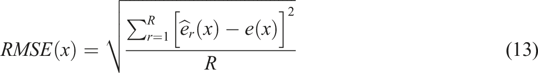
Bias (x) = \frac{\sum_{r = 1}^{R} [{\hat{e}}_{r} (x) - e (x)]}{R}

(12)

RMSE (x) = \sqrt{\frac{{\sum_{r = 1}^{R} [{\hat{e}}_{r} (x) - e (x)]}^{2}}{R}}

(13)

where

{\hat{e}}_{r} (x)

is the estimate for parameter x in the rth dataset, and

e (x)

is the true value of parameter x. To assess classification accuracy, we computed the agreement rates between the estimates obtained under each simulated dataset and the true values for each attribute and attribute profile.

Table 2 lists the descriptive statistics for the bias and RMSE for each item parameter in the SDCM. On average, the bias estimates were all around 0, suggesting that the SDCM can provide unbiased parameter estimates. Among them, the bias and RMSE for the main effect estimates of the potentially unordered option (i.e.,

λ_{1, i, v}

) were larger.

Table 2.

Bias and RMSE of the Estimated Item Parameters of the SDCM in Simulation Study 1.

Bias	$λ_{0, i, r_{2}}$	$λ_{0, i, r_{3}}$	$λ_{0, i, r_{4}}$	$λ_{1, i}$	$λ_{0, i, v}$	$λ_{1, i, v}$
Min	−0.102	−0.070	−0.027	−0.121	−0.061	−0.205
Mean	−0.045	0.043	0.061	−0.048	−0.009	−0.101
Max	0.033	0.142	0.168	0.030	0.046	0.037
SD	0.028	0.039	0.036	0.033	0.018	0.061
RMSE	$λ_{0, i, r_{2}}$	$λ_{0, i, r_{3}}$	$λ_{0, i, r_{4}}$	$λ_{1, i}$	$λ_{0, i, v}$	$λ_{1, i, v}$
Min	0.368	0.376	0.425	0.421	0.460	0.662
Mean	0.503	0.593	0.631	0.582	0.614	0.936
Max	0.622	0.783	0.852	0.769	0.764	1.261
SD	0.064	0.087	0.095	0.080	0.073	0.122

We then compared the results of the SDCM and the ORDM. In terms of model fit, the mean LOOIC values for the SDCM and the ORDM were 70.6 and 78.0, respectively, suggesting that the SDCM fit better than the ORDM. We also compared the classification accuracy at each attribute and profile level for the two models in Tables 3 and 4. For the SDCM, the mean classification accuracy for each attribute was around 0.99, and the mean profile classification accuracy was 0.92, suggesting that the SDCM can provide accurate examinee classifications. For the ORDM, the mean classification accuracy for each attribute was around 0.72, and the mean profile classification accuracy was 0.55. The large discrepancy between the SDCM and the ORDM classification results tells us that, fitting the ORDM to item data that may have a mix of ordered and unordered response options will likely produce a lot of classification errors.

Table 3.

Descriptive Statistics for Attribute and Profile Classification Accuracy of the SDCM in Simulation Study 1.

	$α_{1}$	$α_{2}$	$α_{3}$	$α_{4}$	Profile
Min	0.933	0.912	0.927	0.901	0.752
Mean	0.995	0.996	0.990	0.982	0.924
Max	1.000	1.000	1.000	1.000	1.000
SD	0.009	0.010	0.009	0.012	0.047

Table 4.

Descriptive Statistics for Attribute and Profile Classification Accuracy of the ORDM in Simulation Study 1.

	$α_{1}$	$α_{2}$	$α_{3}$	$α_{4}$	Profile
Min	0.636	0.609	0.624	0.617	0.413
Mean	0.712	0.731	0.705	0.722	0.548
Max	0.818	0.829	0.834	0.810	0.642
SD	0.014	0.012	0.014	0.016	0.061

Study 2: ORDM is the True Model

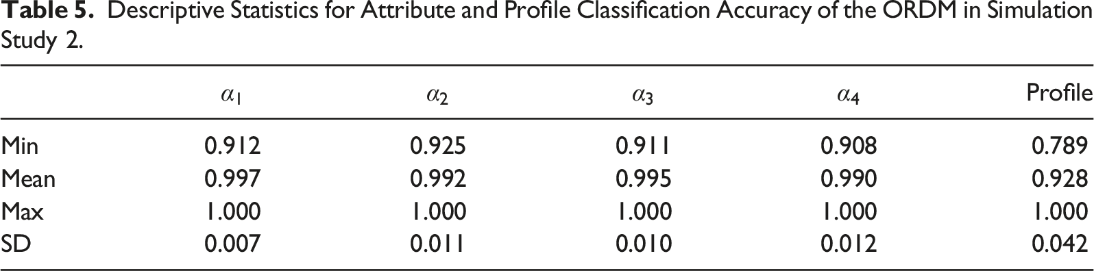
The second simulation study aims to investigate the appropriateness of fitting the SDCM even if the response options were ordered.

We generated 100 datasets using R (R Core Team, 2019) through a similar procedure used in Study 1. The difference is that the item and person parameters were submitted to the ORDM to obtain the probability, and hence the actual response for each person. Both the SDCM and the ORDM were fitted to each dataset. Although the item parameter estimates were not directly comparable due to the different model structures, we can compare the results of fit indices and classification accuracy. In terms of model fit, the mean LOOIC values for the SDCM and the ORDM were 72.9 and 70.8, respectively. This suggests that the ORDM fit better than the SDCM. Results of classification accuracy are shown in Table 5 for the ORDM, and Table 6 for the SDCM. From Table 5, we can see that the classification results for the ORDM were very accurate, with a mean attribute-wise classification accuracy of 0.99, and profile-wise classification accuracy of 0.93. This is expected because the data was generated under the ORDM. Our main interest in Study 2 is the results in Table 6, which shows the classification accuracy of the SDCM when the data was generated under the ORDM. On average, the attribute-classification accuracy was 0.95, and the profile-wise classification accuracy was 0.81. Compared to the results in Study 1, we can see that the drop in classification accuracy was less severe when the SDCM was fitted to ORDM-generated data. When the model and data mismatch, the drop in attribute-wise classification accuracy was 4.0%, and the profile-wise drop was 12.5% in Study 2. In Study 1, the attribute-wise drop was 27.3%, and the profile-wise drop was 40.6%, representing a drop of roughly four times than those in Study 1. In addition, when the SDCM was fitted to the dataset generated under the ORDM in Study 2, we were able to achieve 100% classification accuracy in some iterations. Compared to Study 1, the maximum classification accuracy under the model-data mismatch was around 82.2%.

Table 5.

Descriptive Statistics for Attribute and Profile Classification Accuracy of the ORDM in Simulation Study 2.

	$α_{1}$	$α_{2}$	$α_{3}$	$α_{4}$	Profile
Min	0.912	0.925	0.911	0.908	0.789
Mean	0.997	0.992	0.995	0.990	0.928
Max	1.000	1.000	1.000	1.000	1.000
SD	0.007	0.011	0.010	0.012	0.042

Table 6.

Descriptive Statistics for Attribute and Profile Classification Accuracy of the SDCM in Simulation Study 2.

	$α_{1}$	$α_{2}$	$α_{3}$	$α_{4}$	Profile
Min	0.882	0.891	0.893	0.876	0.711
Mean	0.953	0.955	0.947	0.949	0.812
Max	1.000	1.000	1.000	1.000	1.000
SD	0.015	0.014	0.016	0.018	0.057

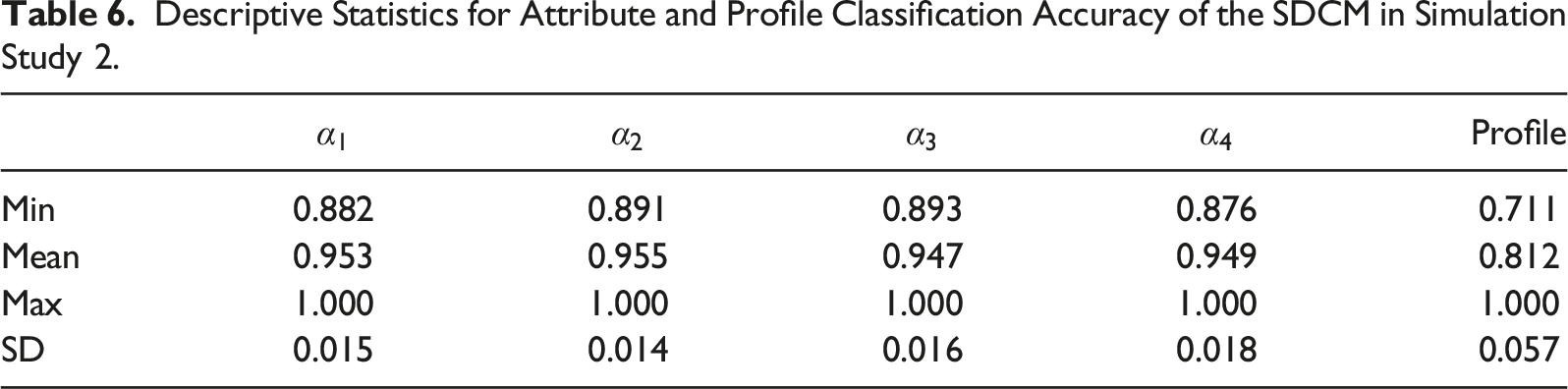
To sum up, classification accuracy was higher when the model matches the data structure. When there was a mismatch, the SDCM performed better than the ORDM, as demonstrated by SDCM’s smaller decrease in classification accuracy.

Discussion

When response options are all ordered, ordinal DCMs such as the ORDM could be directly applied to calibrate the item responses. However, we sometimes provide a “Neither Agree nor Disagree,” “Neutral,” “Don’t Know,” “No Opinion,” or “Hard to Say” option for respondents to select when appropriate. Although this makes the modeling process more difficult and complex, we should appreciate incorporating those potentially unordered options. Without those options, respondents would be forced to select an option that they don’t intend to, and this would add noise to our estimation of their latent traits. The SDCM that we proposed in this study, based on the semi-ordered IRT models developed by Huggins-Manley et al. (2018), successfully incorporates both the ordered and potentially unordered options into the estimation.

Through the operational study, we demonstrated that the SDCM produced smaller average standard errors than the ORDM for the ordinal scale item parameters. We also provided example item characteristic curves to help readers understand different patterns. Although we may be able to infer whether an option of interest may or may not be ordered, depending on the similarities of the curves between the SDCM and the ORDM, the primary purpose of a measurement model is to accurately measure individuals’ latent traits. Through simulation study 1, we found that the SDCM could provide unbiased parameter estimates and accurate individual classifications. We also found that fitting the ORDM to item data from a mix of ordered and unordered response options led to a lot of classification errors. Through simulation study 2, we found that fitting the SDCM to item data from fully ordered response options led to relatively fewer classification errors. In practice, if there are potentially non-ordered responses options, we recommend readers to fit both the SDCM and the ORDM, so that model fit results and classification agreement between the models can be compared, similar to what we have done in the operational study.

The operational and simulation studies lead to our thoughts on the following research questions which could be further explored in the future. First, fit evaluation for polytomous DCM item responses is needed. As discussed in the results section, the results of absolute and relative fit indices may be affected by the selection of prior distributions. Using the same prior for both the SDCM and the ORDM, we found that the SDCM fit better than the ORDM in terms of overall model fit and item fit. More research is needed on the ability of the indices to select the “true” model. In addition to model fit and item fit, we would also want to include person fit information into consideration. In the DCM area, studies on person fit (e.g., Liu et al., 2009) have been limited to binary items under specific models. Future research could look into person fit indices for polytomous items.

Second, one could seek to further investigate the effect of the response option distribution on model selection between the SDCM and the ORDM. Researchers could consider factors such as the proportion of people selecting the nominal response option, and the magnitude of correlations between the nominal response option and other related variables.

Third, evaluating the effect of sample sizes for polytomous DCM items is needed. In terms of model complexity, the SDCM is between the ORDM and the NRDM. Thus, the SDCM may require a sample size that is between those two models. However, there is no study on sample size guidelines for either the ORDM or the NRDM. We imagine that sample size is not a standalone issue as it involves factors such as Q-matrix complexity and test length. Future research into sample size requirements for polytomous items would be helpful.

Fourth, in addition to the ORDM, other ordinal DCMs such as the sequential GDINA model (Ma & de la Torre, 2016), the general polytomous diagnosis model (Chen & de la Torre, 2018), the modified ORDM (Liu & Jiang, 2018), and the rating scale DCM (Liu & Jiang, 2020) could be considered as the base for the SDCM, just like how the semi-ordered GPCM could be extended to accommodate other polytomous IRT models.

Lastly, another potential avenue to incorporate the nominal responses into the estimation process is to use the tree approach (e.g., Ma, 2019) or the two-level nesting approach (e.g., Suh & Bolt, 2010; Liu & Liu, 2020) where the first level evaluates the probability of selecting the nominal response option. If the respondent does not select the nominal response option, the second level is activated to estimate the probability of selecting each ordinal response option. This is a theoretically possible approach, and future research could look into this opportunity and compare that with the SDCM.

Supplemental Material

Supplemental Material - Diagnostic Classification Models for a Mixture of Ordered and Non-ordered Response Options in Rating Scales

Supplemental Material for Diagnostic Classification Models for a Mixture of Ordered and Non-ordered Response Options in Rating Scales by Ren Liu, Haiyan Liu, Dexin Shi, and Zhehan Jiang in Applied Psychological Measurement.

Footnotes

Declaration of Conflicting Interests

The author(s) declared no potential conflicts of interest with respect to the research, authorship, and/or publication of this article.

Funding

The author(s) received no financial support for the research, authorship, and/or publication of this article.

ORCID iD

Ren Liu

Supplemental Material

Supplemental material for this article is available online.

References

Ahn

J. R. R.

Feuerstahler

(2021). Diagnostic classification using a polytomous measure of Korean organizational commitment. In Quantitative psychology (pp. 417–427). Springer.

Bejarano

Ahumada

Sánchez

Cadenas

de Marco

Hynes

Cumsille

(2011). Perception of risk and drug use: An exploratory analysis of explanatory factors in six Latin American countries. The Journal of International Drug, Alcohol and Tobacco Research, 1(1), 9–17.

Bock

R. D.

(1972). Estimating item parameters and latent ability when responses are scored in two or more nominal categories. Psychometrika, 37(1), 29–51. https://doi.org/10.1007/bf02291411

Brooks

S. P.

Gelman

(1998). General methods for monitoring convergence of iterative simulations. Journal of Computational and Graphical Statistics, 7(4), 434–455. https://doi.org/10.2307/1390675

Carpenter

Gelman

Hoffman

M. D.

Lee

Goodrich

Betancourt

Brubaker

Guo

Riddell

(2017). Stan: A probabilistic programming language. Journal of Statistical Software, 76(1), 1. https://doi.org/10.18637/jss.v076.i01

Chen

de la Torre

(2018). Introducing the general polytomous diagnosis modeling framework. Frontiers in Psychology, 9, 1474. https://doi.org/10.3389/fpsyg.2018.01474

Coe

C. K.

(1992). The MBTI: Potential uses and misuses in personnel administration. Public Personnel Management, 21(4), 511–522. https://doi.org/10.1177/009102609202100407

Cohn

Huggins-Manley

A. C.

(2020). Applying unidimensional models for semiordered data to scale data with neutral responses. Educational and Psychological Measurement. 80(2), 242–261. 0013164419861143.

Coombs

C. H

(1964). A theory of data. Mathesis Press.

10.

Duane

Kennedy

A. D.

Pendleton

B. J.

Roweth

(1987). Hybrid Monte Carlo. Physics Letters B, 195(2), 216–222. https://doi.org/10.1016/0370-2693(87)91197-x

11.

Gelfand

A. E.

Dey

D. K.

Chang

(1992). Model determination using predictive distributions with implementation via sampling-based methods. In Bernardo

J. M.

Berger

J. O.

Dawid

A. P.

Smith

A. F. M.

(Eds.), Bayesian statistics 4 (pp. 147–167). Oxford University Press.

12.

Gelman

Carlin

J. B.

Stern

H. S.

Dunson

D. B.

Vehtari

Rubin

D. B.

(2013). Bayesian data analysis (third edition). : Chapman & Hall/CRC Press. Ch. 6).

13.

Gelman

Rubin

D. B.

(1992). Inference from iterative simulation using multiple sequences. Statistical Science, 7(4), 457–511. https://doi.org/10.1214/ss/1177011136

14.

Goldberg

L. R.

Johnson

J. A.

Eber

H. W.

Hogan

Ashton

M. C.

Cloninger

C. R.

Gough

H. C.

(2006). The International Personality Item Pool and the future of public-domain personality measures. Journal of Research in Personality, 40(1), 84–96. https://doi.org/10.1016/j.jrp.2005.08.007

15.

Haertel

E. H.

(1989). Using restricted latent class models to map the skill structure of achievement items. Journal of Educational Measurement, 26(4), 301–321. https://doi.org/10.1111/j.1745-3984.1989.tb00336.x

16.

Huggins-Manley

A. C.

Algina

Zhou

(2018). Models for semiordered data to address not applicable responses in scale measurement. Structural Equation Modeling: A Multidisciplinary Journal, 25(2), 230–243. https://doi.org/10.1080/10705511.2017.1376586

17.

Junker

B. W.

Patz

R. J.

van Houdnos

N. M.

(2016). Markov chain Monte Carlo for item response models. Handbook of Item Response TheoryStatistical Tools, 21(1), 271–325.

18.

Junker

B. W.

Sijtsma

(2001). Cognitive assessment models with few assumptions, and connections with nonparametric item response theory. Applied Psychological Measurement, 25(3), 258–272. https://doi.org/10.1177/01466210122032064

19.

Kunina-Habenicht

Rupp

A. A.

Wilhelm

(2009). A practical illustration of multidimensional diagnostic skills profiling: Comparing results from confirmatory factor analysis and diagnostic classification models. Science and Engineering Ethics, 35(2–3), 64–70. https://doi.org/10.1016/j.stueduc.2009.10.003

20.

Liu

Jiang

(2018). Diagnostic classification models for ordinal item responses. Frontiers in Psychology, 9, 2512. https://doi.org/10.3389/fpsyg.2018.02512

21.

Liu

Jiang

(2020). A general diagnostic classification model for rating scales. Behavior Research Methods, 52(1), 422–439. https://doi.org/10.3758/s13428-019-01239-9

22.

Liu

(2020). Nested diagnostic classification models for multiple‐choice items. British Journal of Mathematical and Statistical Psychology, 74(2), 257–285. https://doi.org/10.1111/bmsp.12214

23.

Liu

Shi

(2020). Using diagnostic classification models in psychological rating scales. The Quantitative Methods for Psychology, 16(5), 442–456. https://doi.org/10.20982/tqmp.16.5.p442

24.

Liu

Douglas

J. A.

Henson

R. A.

(2009). Testing person fit in cognitive diagnosis. Applied Psychological Measurement, 33(8), 579–598. https://doi.org/10.1177/0146621609331960

25.

(2019). A diagnostic tree model for polytomous responses with multiple strategies. British Journal of Mathematical and Statistical Psychology, 72(1), 61–82. https://doi.org/10.1111/bmsp.12137

26.

de la Torre

(2016). A sequential cognitive diagnosis model for polytomous responses. British Journal of Mathematical and Statistical Psychology, 69(3), 253–275. https://doi.org/10.1111/bmsp.12070

27.

Madison

M. J.

Bradshaw

L. P.

(2015). The effects of Q-Matrix design on classification accuracy in the log-linear cognitive diagnosis model. Educational and Psychological Measurement, 75(3), 491–511. https://doi.org/10.1177/0013164414539162

28.

Maris

(1999). Estimating multiple classification latent class models. Psychometrika, 64(2), 187–212. https://doi.org/10.1007/bf02294535

29.

Muraki

(1992). A generalized partial credit model: Application of an EM algorithm. Applied Psychological Measurement, 16(1), 159–176. https://doi.org/10.1002/j.2333-8504.1992.tb01436.x

30.

R Core Team (2019). R (version 3.6): R Foundation for Statistical Computing [Computer Software]

31.

Rupp

A. A.

Templin

Henson

R. A.

(2010). Diagnostic assessment: Theory, methods, and applications. Guilford Press.

32.

Schuman

Presser

(1996). Questions and answers in attitude surveys: Experiments on question form, wording, and context. Sage.

33.

Souri

Hosseinpour

Rahmani

A. M.

(2018). Personality classification based on profiles of social networks’ users and the five-factor model of personality. Human-centric Computing and Information Sciences, 8(1), 1–15. https://doi.org/10.1186/s13673-018-0147-4

34.

Suh

Bolt

D. M.

(2010). Nested logit models for multiple-choice item response data. Psychometrika, 75(3), 454–473. https://doi.org/10.1007/s11336-010-9163-7

35.

Tatsuoka

K. K.

(1983). Rule space: An approach for dealing with misconceptions based on item response theory. Journal of Educational Measurement, 20(4), 345–354. https://doi.org/10.1111/j.1745-3984.1983.tb00212.x

36.

Templin

Henson

Rupp

Jang

Ahmed

(2008). Cognitive diagnosis models for nominal response data. Annual Meeting of the National Council on Measurement in Education, New Brunswick, New Jersey, October, 2008.

37.

Templin

J. L.

Henson

R. A.

(2006). Measurement of psychological disorders using cognitive diagnosis models. Psychological Methods, 11(3), 287–305. https://doi.org/10.1037/1082-989x.11.3.287

38.

Thissen

(1991). MULTILOG user's guide: Multiple, categorical item analysis and test scoring using item response theory. Scientific Software International.

39.

Thissen

Steinberg

(1986). A taxonomy of item response models. Psychometrika, 51(4), 567–577. https://doi.org/10.1007/bf02295596

40.

Vehtari

Gelman

Gabry

(2017). Practical Bayesian model evaluation using leave-one-out cross-validation and WAIC. Statistics and Computing, 27(5), 1413–1432. https://doi.org/10.1007/s11222-016-9696-4

41.

Zhou

Huggins-Manley

A. C.

(2020). The performance of the semigeneralized partial credit model for handling item-level missingness. Educational and Psychological Measurement, 80(6), 1196–1215. https://doi.org/10.1177/0013164420918392

Supplementary Material

Please find the following supplemental material available below.

For Open Access articles published under a Creative Commons License, all supplemental material carries the same license as the article it is associated with.

For non-Open Access articles published, all supplemental material carries a non-exclusive license, and permission requests for re-use of supplemental material or any part of supplemental material shall be sent directly to the copyright owner as specified in the copyright notice associated with the article.

0.00 MB

0.44 MB